| Issue |
A&A
Volume 651, July 2021
|
|
|---|---|---|
| Article Number | A8 | |
| Number of page(s) | 22 | |
| Section | Interstellar and circumstellar matter | |
| DOI | https://doi.org/10.1051/0004-6361/202040082 | |
| Published online | 01 July 2021 | |
Multifrequency high spectral resolution observations of HCN toward the circumstellar envelope of Y Canum Venaticorum
1
Molecular Astrophysics Group, Instituto de Física Fundamental, IFF-CSIC,
C/Serrano, 123,
28006
Madrid,
Spain
e-mail: jpablo.fonfria@csic.es
2
SOFIA-USRA, NASA Ames Research Center,
MS 232-12,
Moffett Field,
CA
94035,
USA
3
Physics Department – UC Davis,
One Shields Ave.,
Davis,
CA
95616,
USA
4
Astronomy Department, University of Texas,
Austin,
TX
78712,
USA
5
Southwest Research Institute,
San Antonio,
TX
78228,
USA
6
Observatorio Astronómico Nacional, OAN-IGN,
Alfonso XII, 3,
28014
Madrid,
Spain
Received:
7
December
2020
Accepted:
5
May
2021
High spectral resolution observations toward the low mass-loss rate C-rich, J-type asymptotic giant branch (AGB) star Y CVn were carried out at 7.5, 13.1, and 14.0 μm with the Echelon-cross-echelle Spectrograph mounted on the Stratospheric Observatory for Infrared Astronomy and the Texas Echelon-cross-echelle Spectrograph on the Infrared Telescope Facility. Around 130 HCN and H13CN lines of bands ν2, 2ν2, 2ν2 − ν2, 3ν2 − 2ν2, 3ν2 − ν2, and 4ν2 − 2ν2 were identified involving lower levels with energies up to ≃3900 K. These lines were complemented with the pure rotational lines J = 1−0 and 3–2 of the vibrational states up to 2ν2 acquired with the Institut de Radioastronomie Millimétrique 30 m telescope, and with the continuum taken with Infrared Space Observatory. We analyzed the data in detail by means of a ro-vibrational diagram and with a code written to model the absorption and emission of the circumstellar envelope of an AGB star. The continuum is mostly produced by the star with a small contribution from dust grains comprising warm to hot SiC and cold amorphous carbon. The HCN abundance distribution seems to be anisotropic close to Y CVn and in the outer layers of its envelope. The ejected gas is accelerated up to the terminal velocity (≃8 km s−1) from the photosphere to ≃3R⋆, but there is evidence of higher velocities (≳9–10 km s−1) beyond this region. In the vicinity of the star, the line widths are as high as ≃10 km s−1, which implies a maximum turbulent velocity of 6 km s−1 or the existence of other physical mechanisms probably related to matter ejection that involve higher gas expansion velocities than expected. HCN is rotationally and vibrationally out of local thermodynamic equilibrium throughout the whole envelope. It is surprising that a difference of about 1500 K in the rotational temperature at the photosphere is needed to explain the observations at 7.5 and 13–14 μm. Our analysis finds a total HCN column density that ranges from ≃2.1 × 10¹⁸ to 3.5 × 1018 cm−2, an abundance with respect to H2 of 3.5 × 10⁻⁵ to 1.3 × 10⁻⁴, and a 12C/13C isotopic ratio of ≃2.5 throughout the whole envelope.
Key words: stars: AGB and post-AGB / stars: individual: Y CVn / circumstellar matter / stars: abundances / line: identification / surveys
© ESO 2021
1 Introduction
The structure, kinematics, and chemistry of circumstellar envelopes (CSEs) of the asymptotic giant branch (AGB) stars have been explored since the second half of the last century. These variable stars return processed matter to the interstellar medium by a combination of the pulsation of their atmospheres, which creates the foundation of the CSE, and the formation of dust grains as a consequence of the gas cooling that subsequently occurs in this environment (e.g., Goldreich & Scoville 1976; Bowen 1988; Decin et al. 2006). The development of these winds are tightly related to the chemical evolution of the expelled gas, which depends on the C/O abundance ratio (e.g., Agúndez et al. 2020). Carbon rich stars (C-rich) are defined as those with CSEs where C/O > 1, the envelopes of oxygen rich stars (O-rich) show C/O < 1, and the S-type stars have CSEs where C/O ≃1. Most of what we know about these environments is derived from the study of IRC+10216 (the C-rich CSE around the star CW Leo; e.g., Keady et al. 1988, 1993; Cernicharo et al. 2000; Fonfría et al. 2008; Agúndez et al. 2012), IK Tau (O-rich; e.g., Velilla-Prieto et al. 2017; Decin et al. 2018a,b), or W Aql (S-type; e.g., Danilovich et al. 2014; Ramstedt et al. 2017; De Beck & Olofsson 2020), with mass-loss rates of ≃2.7 × 10⁻⁵, 2.0 × 10⁻⁵, and 2.7 × 10⁻⁶ M⊙ yr−1, respectively (Ramstedt & Olofsson 2014; Guélin et al. 2018).
The envelopes of these high mass-loss rate stars are prime locations to search for new molecules, investigate the dust density distribution, or look for gas structures (e.g., Mauron & Huggins 1999; Cernicharo et al. 2000, 2015a,b, 2019a,b; Leão et al. 2006; Agúndez et al. 2008; De Beck et al. 2013; Jeffers et al. 2014; Velilla-Prieto et al. 2017). Nevertheless, investigating the inner layers of the envelopes, where the gas is accelerated (r ≃ 1–30R⋆; e.g., Decin et al. 2006; Fonfría et al. 2008), has remained hampered because of the increased density of gas and dust in this region and the demanding angular resolution requirements. Recent observations of vibrationally excited lines in addition to the large capacities of the Atacama Large Millimeter Array (ALMA) and the Very Large Telescope Interferometer (VLTI) are shedding light on this problem (e.g., Fonfría et al. 2008, 2019; Cernicharo et al. 2011; Agúndez et al. 2012; Vlemmings et al. 2017; Adam & Ohnaka 2019; Ohnaka et al. 2019).
Meanwhile, low mass-loss rate stars (~ 10−7 M⊙ yr−1) are, typically, much brighter in the optical and the near-IR because of their thinner CSEs. This allows us to directly observe the central stars and inner layers of their envelopes. However, the complexity of the electronic molecular transitions has limited the community to use these observations to understand the kinematics and chemistry close to their central stars with few exceptions. Hinkle (1978) and Hinkle & Barnes (1979a,b) analyzed the gas kinematics of the extended atmosphere of the O-rich star R Leo, with a mass-loss rate of 1.0 × 10⁻⁷ M⊙ yr−1 (Ramstedt & Olofsson 2014). However, the molecular emission and gas kinematics of the extended atmosphere, and even the first tens of stellar radii beyond, with no C-rich counterpart was studied in detail as far as we know. A step was taken in this direction with V Oph, whose C2 H2 absorption between 8 and 9 μm was studied with low spectral resolution interferometer observations (Ohnaka et al. 2007) to roughly determine the abundance and excitation temperature of this molecule near the photosphere.
About 10–15% of C-rich stars are J-type stars (Abia & Isern 2000; Morgan et al. 2003). These stars show a significant enhancement of the 13C abundance with respect to the main carbon isotopologue (12 C/13C ≲ 15; Abia & Isern 1997; Ohnaka et al. 1999), compared to the typical ratio found for most C-rich stars (R-, N-, and CH-type, 30 ≲ 12C/13C ≲ 100; Lambert et al. 1986; Keenan 1993; Chen et al. 2007). The Li abundance is usually higher than expected (e.g., Gordon 1971; Abia & Isern 1997; Hatzidimitriou et al. 2003) and heavy elements associated with s-processes are barely present in their atmospheres (e.g., Dominy 1985). Most of J-type stars are irregular or semiregular (Abia & Isern 2000) and their mass-loss rates are usually low (Lorenz-Martins 1996). The origins of J-type stars seem to be different to those of typical C-rich (N stars) and SC stars, that is, those which are presumably evolving from S-type to C-rich (Abia et al. 2020). Several hypotheses were proposed to explain the peculiarities of these stars, such as that they are evolving independently to ordinary carbon stars (Lorenz-Martins 1996) or they are the descendants of low mass R stars (Abia et al. 2003). Nevertheless, there is not a satisfactory explanation to their existence thus far.
Y CVn is a C-rich J-type semiregular b (SRb) star (e.g., Abia & Isern 2000) that is located at ≃ 310 ± 17 pc from Earth (Gaia Early Data Release 3 (EDR3); Gaia Collaboration 2016, 2021). Its mass-loss rate at this distance is ≃ 1.4 × 10⁻⁷ M⊙ yr−1 based on the results of Ramstedt & Olofsson (2014) (≃ 1.5 × 10⁻⁷ M⊙ yr−1 for a distance of 321 pc). It was observed in the past many times at different spectral resolutions between the optical and millimeter ranges (e.g., Lambert et al. 1986; Olofsson et al. 1993a,b; Bachiller et al. 1997; Schilke & Menten 2003; Yang et al. 2004; Neufeld et al. 2011; Schöier et al. 2013; Ramstedt & Olofsson 2014; Massalkhi et al. 2018b, 2019). These observations revealed that the CSE of Y CVn displays molecular features from species such as CO, HCN, CN, CS, SiS, SiC2, SiO, C2, C3, CH, and H2 O. Low angular resolution observations (≃ 2′′ –3′′) of HCN(1−0) and CN(1−0) are available(Lindqvist et al. 2000). The HCN emission is point-like due to the compact maser contributions displayed by the J = 1−0 line (e.g., Dinh-V-Trung & Nguyen-Q-Rieu 2000). In contrast, the CN brightness distribution, which is expected to encircle the HCN brightness distribution, is partially resolved, and shows a clumpy, asymmetric structure that peaks at a distance of 1′′ − 2′′ from Y CVn and has a diameter of about 6′′. However, its CSE was not explored in detail and the gas kinematics and the physical andchemical conditions throughout the envelope are poorly known mostly due to the lack of sensitive observations of the gas acceleration region.
In this paper, we present the first high spectral resolution observations in the mid-IR of Y CVn carried out with the Echelon-cross-echelle Spectrograph (EXES; Richter et al. 2018) mounted on the Stratospheric Observatory for Infrared Astronomy (SOFIA; Temi et al. 2018) and with the Texas Echelon-cross-echelle Spectrograph (TEXES; Lacy et al. 2002) mounted on the Infrared Telescope Facility (IRTF), which is located on Maunakea (Hawaii). The analysis of the ro-vibrational spectrum of HCN1 and H13 CN together with new data acquired in the millimeter range with the Institut de Radioastronomie Millimétrique (IRAM) 30 m telescope, placed on Pico Veleta (Spain), allowed us to describe the kinematic behavior of the gas, the physical conditions prevailing throughout the whole envelope, and the abundance distribution of these molecules.
2 Observations
2.1 SOFIA-EXES
Y CVn was observed with EXES on two successive SOFIA flights, which took place 17–18 Apr. 2019 (UT). The first run was conducted while SOFIA flew at an altitude of 12.8 km. We focused on a central wavenumber of 1335 cm−1 (7.5 μm) in the high-low instrument configuration. We nodded Y CVn off of the slit to get to blank sky. The slit was 2′′.4 wide and 2′′.0 long. The full coverage of Y CVn’s spectrum at this wavenumber and observing mode is 1313.7–1358.2 cm−1 (7.362–7.612 μm).
The second observation of Y CVn was on the next flight at an altitude of 13.1 km in the high-medium mode. We used a 2′′.4 wide slit with a length of 21′′.0, so that nodding along the slit was possible. We chose to center the observations around 714.70 cm−1 (14.0 μm), which results in the covered spectral range 712.49–717.70 cm−1 (13.93–14.04 μm).
All EXES data were reduced using the Redux pipeline (Clarke et al. 2015). The median spectral resolving power, R = λ∕Δλ, for the high-low configuration at 7.5 μm was empirically determined to be about 60 000 by fitting several narrow, optically thin telluric features with a Gaussian. This resolving power means a velocity resolution of5.0 km s−1. An R of 67 000 (4.4 km s−1) was found for the high-medium setting at 14.0 μm. Customized procedures were written for the 14.0 μm observationsto extract an extra order at the high frequency edge of the covered range, which only contained our negative beam.
The observations show a forest of molecular lines in the covered spectral range dense enough to make finding a clean baseline difficult. A careful inspection of the spectra suggests that it is affected by a small amplitude, long wavelength ripple that was removed by dividing the data with a cubic spline fit. We found no periodic features or artifacts affecting the line profiles. The resulting normalized spectra together with the identified HCN and H13 CN lines are shown in Figs. 1 and 2 (see a brief description of HCN in Appendix A and a vibrational energy diagram showing the vibrational transitions observed in this work in Fig. A.1). The lines of other molecules are not identified in Figs. 1 and 2 for the sake of clarity. We estimate a noise root mean square (RMS) of ≃ 0.5% of the continuum at 7.5 μm and of ≃2.0% at 14.0 μm. We adopted a systemic velocity in the LSR system of +22.0 km s−1 (Massalkhi et al. 2018b), which implies radial velocities of Y CVn with respect to us at the time of the observations of +24.8 and +25.1 km s−1 at 7.5 and 14.0 μm, respectively.
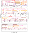 |
Fig. 1 Observed spectrum of Y CVn in the spectral range 13–14 μm (top panels: 14.0 μm, 712.55–717.70 cm−1, SOFIA-EXES; bottom panels: 13.1 μm, 755.50–769.12 cm−1, IRTF-TEXES). The spectra are corrected for the Doppler shift due to the relative movement between the star and the Earth at the time of the observations. The resolving power is R ≃ 67 000 at 14.0 μm and ≃ 83 000 at 13.1 μm, which provides us with a spectral resolution of ≃4.4 and 3.6 km s−1, respectively. Different lines of several vibrational states of HCN (red, orange, and brown) and H13 CN (pink) are found in this spectrum. A model of the atmospheric transmission estimated with the atmospheric transmission calculator ATRAN (Lord 1992) is included in gray. The TEXES data were cleaned from the atmospheric lines with a routine developed by J. H. Lacy. The red and blue curves are the synthetic spectra derived from our spherically symmetric and asymmetric models, respectively. |
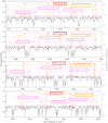 |
Fig. 2 Observed spectrum of Y CVn at 7.5 μm (1313.70–1358.45 cm−1) using SOFIA-EXES. The spectrum is corrected for the Doppler shift due to the star and Earth relative movement at the time of the observations. The resolving power is R ≃ 60 000 which provides us with a spectral resolution of ≃5.0 km s−1. Differentlines of several vibrational states of HCN (red, orange, and violet) and H13 CN (pink) are found in this spectrum. An ATRAN model of the atmospheric transmission is included in gray. The red and blue curves are the synthetic spectra derived from our spherically symmetric and asymmetric models, respectively. |
2.2 IRTF-TEXES
Y CVn was also observed with the Texas Echelon-cross-echelle Spectrograph (TEXES; Lacy et al. 2002) at NASA’s IRTF on Maunakea. These observations took place on 14 Feb 2019 (UT) and were carried out in TEXES’ high-low mode. They have a spectral coverage of 754.66 to 769.18 cm−1 (13.00–13.25 μm). The data were reduced following the methods described in Lacy et al. (2002). The value of R was observationally determined from the data to be 83 000 (or a spectral resolution of 3.6 km s−1). We estimate a noise RMSof ≃2% of the continuum. The relative radial velocity of Y CVn during the observation is estimated to be +3.6 km s−1.
After doing the standard data reduction, we normalized the spectrum and removed the weak and medium strength telluric features by dividing the observed data by an atmospheric transmission model derived from a routine written for TEXES by J. H. Lacy. It relies on thehigh-resolution transmission molecular absorption database (HITRAN; Gordon et al. 2017) and balloon data to account for temperature and humidity against altitude from the Integrated Global Radiosonde Archive project (Durre & Yin 2008)2. This code isstill under development and it cannot be applied to the observations acquired with SOFIA-EXES. Nevertheless, the results of using Lacy’s model are better than what we got by dividing the observations by a telluric calibrator. The spectral ranges blocked by strong telluric lines could not be recovered after the spectra division andthey appear as gaps in Fig. 1. The spectral ranges affected by weaker telluric features that were successfully removed show a higher noise but allow us to use molecular lines seriously contaminated otherwise.
2.3 IRAM 30 m telescope
The Y CVnobservations were taken in 2017 and the first half of 2019 as part of projects 164-15, 155-16, 046-17, and 048-17 (Fig. 3). We used the Eight Mixer Receivers (EMIR) E090 and E230 (Carter et al. 2012) with the FTS200 backends, which provided us with a total bandwidth of 15.7 GHz and a channel width of 0.2 MHz. The weather was good during the observing campaigns with atmospheric opacities below 0.25 at 1 mm and up to 0.05 at 3 mm. The system temperatures were usually below 290 and 75 K, respectively. The noise RMS levels are typically 12 and 7 mK ( ; 100 and 55 mJy) for the lines of HCN and H13CN at 1 mm, respectively, and 2.3 mK (
 ; 14 mJy) for the lines at 3 mm. We used the wobbler switching technique wobbling the secondary mirror at a frequency of 0.5 Hz and with a throw of 90′′. This technique produces very flat baselines that favors the detection of weak lines. We estimate the calibration error to be ≃ 20%. The J = 3−2 lines of HCN and H13CN, observed in different setups, were made compatible by comparing the SiC2 lines 120,12−110,11 and 112,10−102,9, also observed in different setups, whose intensities are expected to be nearly the same (Cernicharo et al. 2012).
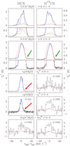 |
Fig. 3 Observed HCN and H13CN lines of Y CVn with the IRAM 30 m telescope (black histograms). The red and blue curves are the synthetic lines derived from the spherically symmetric (red) and asymmetric (including maser emission; blue) envelope models. The red and green arrows point to red-shifted wings that cannot be reproduced with our spherically symmetric envelope model. The small insets in the boxes with the v = 0 J = 1− 0 and 3–2lines zoom in to show the line profiles close to the baseline (Sect. 4.2). The green profiles for these lines were calculated with the asymmetric envelopemodel without considering maser emission (Sect. 5.2.1). The H13 CN lines |


2.4 ISO-SWS and LWS
These data sets were complemented with previous low spectral resolution observations acquired with the Infrared Space Observatory (ISO) (Hony et al. 2002; Yang et al. 2004), which operated from 1995 to 1998, to derive the overall properties of the infrared continuum source of Y CVn. This facility was able to take infrared spectra with the Short Wavelength Spectrometer (SWS; 2.5–45 μm) and the Long Wavelength Spectrometer (LWS; 45–200 μm). Y CVn was observed with both spectrographs (TDT numbers: 16000926 and 19500730) and the grating modes S01 and L01, which gave effective resolving powers of 500 at 35 μm and 200–300 above 45 μm, respectively (de Graauw et al. 1996; Yang et al. 2004). The flux calibration of this spectrum was checked against observations of different catalogs (Two Micron All Sky Survey (2MASS), AKARI/IRC All-Sky Survey (AKARI), Diffuse Infrared Background Experiment (DIRBE), Infrared Astronomical Satellite (IRAS), Wide-field Infrared Survey Explorer (WISE), and the unblurred coadds of the WISE imaging (unWISE) Point Source Catalogs; Neugebauer et al. 1984; Smith et al. 2004; Skrutskie et al. 2006; Ishihara et al. 2010; Wright et al. 2010; Lang 2014). The deviation is within the estimated uncertainties of 20% for the ISO data but we scaled this spectrum to get the best agreement.
3 Modeling
3.1 Envelope model
The envelope was divided into three different regions (I, II, and III) with inner radii Ri = 1R⋆, Rii, and Riii (see Table 1), where changes in important quantities such as the gas expansion velocity field and the formation of dust grains may occur. The abundances of HCN and H13 CN were considered as zero beyond the photodissociation radius, Rph, which is a free parameter (Table 2). The properties of the Y CVn CSE are poorly known due to the limited work that focusedon this low mass-loss rate star. Nevertheless, some parameters were previously well determined and they were adopted as fixed in this work (Table 1; nonfree parameters). Others were taken from the literature as initial guesses for our model. Necessary quantities absent in the literature were adopted to be equal to those derived from other sources. Spherical symmetry was initially assumed for all the physical and chemical quantities.
A terminal gas expansion velocity of 8–9 km s−1 (Izumiura et al. 1995; Ramstedt & Olofsson 2014) along with a turbulent line width of 1 km s−1 as in the C-rich AGB star IRC+10216 (Fonfría et al. 2008; Agúndez et al. 2012) throughout the whole envelope, and a stellar effective temperature of 2760 K (Bergeat et al. 2001) were initially considered. We adopted the gas kinetic temperaturedependence in the CSE of Y CVn as a function of the distance from the central star, which to first order approximation (the temperature at the photosphere of Y CVn is a free parameter) is derived from the outer envelope of IRC+10216 as it is reasonably well known (Guélin et al. 2018). This region of the CSE of IRC+10216 is as rarefied as the envelope of Y CVn and both envelopes are chemically similar (see Sect. 5.2.6 for a discussion about this assumption). We considered vibrational temperatures between vibrational states affected by ℓ-doubling (for instance, 2ν2(δ) − 2ν2(σ+), ΔEvib ≃ 30 K) to be equal to the kinetic temperature unless different values are necessary. The gas density was derived from the mass conservation law throughout the whole CSE, which implies that  , where vexp is the gas expansion velocity and it can depend on the distance from the star.
The dust grains were assumed to be composed of amorphous carbon (AC) and silicon carbide (SiC), as these materials explain most of the continuum emission at wavelengths below ≃ 30 μm in C-rich AGB stars (e.g., Keady et al. 1988; Hony et al. 2002; Swamy 2005). We considered that carbon-bearing molecules (probably C2 and C3) are able to condense into the carbonaceous material that compose the dust grains (see Fig. 5 of Agúndez et al. 2020) at the starting point of ≃2R⋆ from the center of Y CVn. Solid state SiC is expected to form due to the condensation of Sin Cm molecules on the carbonaceous seeds at the position of the envelope where the kinetic temperature is ≃ 1300 K, that is reached at ≃3R⋆ from the center of the star (Gobrecht et al. 2017; Agúndez et al. 2020). The density and temperature of dust grains were assumed to follow the power laws ∝ r−2, typical of isotropic expansions, and ∝ r−0.4 (Sopka et al. 1985), respectively.
Dust grains are expected to be small in expanding, rarefied winds where the low gas density hampers the dust coagulation (e.g., Hirashita 2000). We thus assumed small, spherical dust grains with a radius of 0.05 μm and a density of 2.5 g cm−3. Scattering was not included because it can be considered to be negligible at wavelengths longer than 5 μm for dust grains with a diameter ≲1 μm.
Nonfree parameters involved in the fits.
3.2 The ro-vibrational diagram
A molecular ro-vibrational line produced by an isotropically expanding envelope usually shows a P Cygni profile, which comprises an absorption component and an emission one typically overlapped. The optical depth of the absorption component of an observed line, which is produced by the molecules in front of the continuum source (the star and the surrounding dust), can be described with this formula (see Appendix B):
![\begin{equation*}\ln\left[\frac{W\nu^28\pi c}{A_{\textrm{ul}}g_{\textrm{u}} N_{\textrm{col,0}}}\right]\simeq y_0-\frac{hcE_{\textrm{rot,low}}}{k_{\textrm{B}}T_{\textrm{rot}}}, \end{equation*}](/articles/aa/full_html/2021/07/aa40082-20/aa40082-20-eq4.png) (1)
(1)
where W is the optical depth associated to the absorption component integrated over the frequency (cm−1), ν is the rest frequency (cm−1), Erot,low the rotational energy of the lower level involved in the transition, and Trot the rotational temperature of the lower vibrational state. The constant Ncol,0 is an arbitrary scaling factor to geta dimensionless argument for the logarithm. Equation (1) holds for all the lines of a given ro-vibrational band. We define the quantity y0 as:
![\begin{equation*}y_0=\ln\left[\frac{N_{\textrm{col}}}{N_{\textrm{col,0}}Z}\right]-\ln\left[\frac{\textrm{e}^{hcE_{\textrm{vib,low}}/k_{\textrm{B}}T_{\textrm{vib},l}}}{1-\textrm{e}^{-hc\bar\nu/k_{\textrm{B}}T_{\textrm{vib,ul}}}}\right], \end{equation*}](/articles/aa/full_html/2021/07/aa40082-20/aa40082-20-eq5.png) (2)
(2)
where Ncol is the column density, Z the total partition function (Z ≃ ZrotZvib),  is the mean frequency of the considered lines, Evib,low the vibrational energy of the lower vibrational state, and Tvib,l and Tvib,ul describe the populations of the lower vibrational state and the upper one with respect to the lower via Boltzmann factors, respectively.
Fitting the data derived from all the lines in a band with Eq. (1) we can estimate the rotational temperature of this band from the slope and the column density from the y-intercept, y0 (Eq. (2)). We note that the data sets related to different hot bands or overtones display y-intercepts offset with respect to that of the fundamental bands due to the effect of the vibrational temperatures.
Free parameters involved in the fits.
3.3 Radiative transfer code
The ro-vibrational diagram gives rough estimates of the molecular excitation and the column density of a given molecule but a more detailed description of the envelope requires the use of more sophisticated methods. We analyzed the continuum and the molecular spectra with the aid of the radiation transfer code developed by Fonfría et al. (2008) to model spherically symmetric CSEs (1D) and improved by Fonfría et al. (2014) to deal with asymmetric envelopes (3D). This code solves the radiation transfer problem in a circumstellar envelope composed of molecular gas, dust grains, and a central continuum source. More information about it, the adopted spectroscopic data and optical properties of dust grains, as well as of the uncertainties of the parameters can be found in the Appendix C and in the papers previously cited.
All the lines of each molecule were fitted simultaneously. The success of the fit was checked by eye. The high line density in the spectra (Figs. 1 and 2), which is frequently seen as a partial contamination of the line to be fitted by other features, together with the high variety of intensities of the observed HCN lines prevented us to use an automatic process based on the minimization of the χ2 function. The general agreement between the automatically calculated best fit and the observations was always poorer. The number of free parameters involved in the fitting process was usually high (see Table 2) but many lines were fitted at the same time. Moreover, the observed lines could be gathered in different groups with particular properties (vibrational states involved or formation region, for instance) and usually only a few parameters directly affected each group of lines while the rest of themhad a limited impact.
4 Results
4.1 The continuum emission
The spectral energy distribution (SED) of Y CVn is single-peaked and the maximum emission is reached at ≃ 1.9 μm (Fig. 4). It decreases monotonically with increasing wavelength except for a few molecular bands. Considering that the mass-loss rate of this star is ~ 10−7 M⊙ yr−1 and that thegas-to-dust ratio is ≃500 (Schöier & Olofsson 2001; Massalkhi et al. 2018b, 2019), the SED described by the ISO observations is very probably dominated by the stellar continuum emission at short wavelengths.
The continuum was fitted with our code in the wavelength range ≃ 2.5−26 μm. We took parameters derived from IRC+10216 (e.g., Fonfría et al. 2008, 2015) as initial guesses. No gas phase molecular species was considered in this fit and the molecular bands were not reproduced. The results can be found in Fig. 4 and the derived parameters in Table 2. The continuum emission from 2.5 to 9 μm is compatible with the emission of a black body with a temperature of about 2900 K. The clear SiC solid state band at 11.3 μm reveals the presence of dust grains composed of this material. Below 2.5 μm, the synthetic continuum departs from the observations. This disagreement is likely a direct consequence of the strong photospheric C2 and CN absorption bands present below 2 μm in the near-IR and the optical ranges typical of J-type stars (e.g., Barnbaum 1994; Ohnaka et al. 1999; Massalkhi et al. 2018a) that were not included in our model.
The SiC solid state band is only slightly sensitive to temperature changes and the SiC absorption is comparatively negligible at any other wavelength. However, the observed and synthetic SEDs are in better agreement when the condensation temperature is around 1000 K than when it is of a few hundreds of K. Fixing the SiC condensation radius to a physically acceptable value is therefore necessary to propose an envelope model. The addition of AC to the model with a dust temperature on the order of 1000 K produces a bump at 8–10 μm that makes the model deviate significantly from the ISO observations. The only scenario that we found to satisfactorily explain the overall emission beyond 2.5 μm considers dust grains made of amorphous SiC with a contribution of AC at a temperature of a few hundred K.
Our results suggest that it is not possible to find a model that accounts for the emission excess beyond 15 μm without considering an opacity increase directly related to AC from ≃100R⋆ to 500R⋆. The best fit is achieved with such an increase located at ≃200R⋆, where the density of dust grains is enhanced by a factor of 15 with respect to the density resulting from a constant dust mass-loss rate. Further opacity increases related to colder dust may be necessary to explain the continuum around 100 μm, which could be related to the extended dusty shell with an inner radius of ≃ 3′ discovered long ago with IRAS (Young et al. 1993; Izumiura et al. 1996; Libert et al. 2007; Cox et al. 2012a,b).
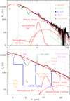 |
Fig. 4 Continuum of Y CVn as observed with ISO (black histogram). The red solid curve is the fit to the observations after the removal of the molecular bands (Table 2). The red dotted curve is the stellar contribution, the red dashed curve the contribution of SiC, and the dotted-dashed one the contribution of amorphous carbon. The red stars, green triangles, blue squares, and magenta circles in the upper panel are photometric measures of the continuum available in different point source catalogs (2MASS, DIRBE, AKARI, IRAS, and WISE – the WISE fluxes at 3.35 and 4.60 μm are clear outliers and they are discarded to use the unWISE values instead). The band identifications in the lower panel are in agreement with previous observations of Y CVn and IRC+10216 (Cernicharo et al. 1999; Yang et al. 2004). |
4.2 The molecular emission
The observed infrared spectra contain a forest of lines of different molecules. In the 13–14 μm range, the spectrum is dominated by broad features with strong emission components and weaker absorptions, typical of P Cygni profiles coming from molecules with a high vibrational temperature. There are also weaker lines showing P Cygni profiles and other lines only in absorption. Around 7.5 μm the spectrum is crowded with absorption lines.
Most of the lines in both spectral ranges come from HCN, C2 H2, and CS, in addition to their 13C-substituted isotopologues, as expected to happen in a J-type star such as Y CVn (12 C/13C ≃ 3; e.g., Abia et al. 2017). The observations contain high-J CS lines of the v = 2−1 and 3–2 bands involving lower levels with energies up to ≃7500 K formed in the stellar photosphere. The HCN lines belong to bands ν2 (π), 2ν2 (σ+), 2ν2 (σ+) − ν2(π), 2ν2 (δ) − ν2(π), 3ν2 (π) − ν2(π), 3ν2 (π) − 2ν2(σ+), 3ν2 (π) − 2ν2(δ), 3ν2 (ϕ) − 2ν2(δ), 4ν2 (σ+) − 2ν2(σ+), and 4ν2 (δ) − 2ν2(δ), and involve lower levels with energies up to ≃3900 K. The apparently different vibrational excitation of CS and HCN might be an optical thickness effect related to the significantly higher Einstein coefficients of the CS lines in the observed spectral range (Aul ≲ 40 s−1) compared to those of the HCN lines (Aul ≲ 4 s−1, see the Exomol database; Tennyson et al. 2016), but other explanations such as the existence of a low HCN abundance gap near the stellar photosphere cannot be ruled out. We also identified C2 H2 lines of different bands up to ν4 + 3ν5(δu) − 2ν5(δg), which involve lower levels with energies ≲ 2900 K. No SiS lineswere detected even though its spectrum is partially covered by our observations. There are still several unidentified features. Some of them are probably lines of higher excitation hot bands of CS, HCN, and C2 H2 but some features could be lines of other molecules.
The width at the baseline of the HCN ro-vibrational lines of the fundamental band ν2 (π) (at ≃ 715 cm−1) is ≃ 0.06–0.08 cm−1, about twiceas high as for lines produced by gas expanding at 7.0–9.0 km s−1 (e.g., Olofsson et al. 1993a; Izumiura et al. 1995; Schöier & Olofsson 2000; Ramstedt & Olofsson 2014; Massalkhi et al. 2018b), which would be of ≃ 0.04 cm−1 considering the resolving power of the spectrograph. This implies maximum gas expansion velocities ≳ 13 km s−1 or local line widths at least as high as ≃ 10 km s−1 (see Sect. 5.2.2).
As shown above, the continuum of Y CVn is dominated by the central star at 7.5 and 13–14 μm and we can assume that the absorption components of all the ro-vibrational lines (Figs. 1 and 2) are constrained to be produced in a region as small as ≃0′′.014 (≃ 2R⋆) to first approximation. With this in mind, we did a ro-vibrational diagram for the absorption components of the HCN lines that can be found in Fig. 5.
The fits to the absorption components were done by adopting the function e −τν, where  ,
,  , and FWHD is the full width at half depth of the component. In the fits to the P Cygni profiles we added the function
  to fit the emission components at the same time as the absorptions (see Appendix B). The τν and
  are different and involve also different Doppler shifts.
The total data set plotted in Fig. 5 contains the opacities of the more isolated, unperturbed lines of several different bands: 2ν2(σ+), 3ν2 (π) − ν2(π), 4ν2 (σ+) − 2ν2(σ+), and 4ν2 (δ) − 2ν2(δ) at 7.5 μm, and ν2(π), 2ν2 (σ+) − ν2(π), and 2ν2 (δ) − ν2(π) at 13–14 μm. All the ro-vibrational bands at 7.5 and 13–14 μm separately are compatible between them except 4ν2(σ+) − 2ν2(σ+), which showsa growing dependence with the increasing rotational energy and thus a negative rotational temperature. We suspect that these lines are affected by either radiation transfer mechanisms not considered in our analysis or errors in the spectroscopic data (see Sect. 5.2.6). Consequently, we did not use the lines of this band in the fits.
The ro-vibrational diagram discloses the existence of four different HCN populations, cold, warm, hot, and very hot, with rotational temperatures of 100 ± 30, 480 ± 110, 1300 ± 270, and 3300 ± 2700 K. The poor accuracy of the temperature of the very hot population is due to the high dispersion inherited from lines with a poorer S/N. The Q branches, even though they are almost completely covered by our observations, are ineffective to study cold gas in the outer envelope due to the typical width of the lines, which is significantly larger than the line separation as the rotational number decreases.
The strong vibrational excitation undergone by HCN implies a significant population in at least four vibrational states (from the ground state up to the 3ν2 state) and four different vibrational temperatures. These temperatures, which are unknown a priori and hard to determine for most of the states from the ro-vibrational diagram due to the data dispersion, make it difficult to estimate the vibrational partition function of HCN, Zvib. Therefore, we can only derive lower and upper limits for the column density.
The lower limits are (4.4 ± 2.6) × 1016, (5.2 ± 1.7) × 1016, (3.5 ± 1.0) × 1017, and (1.4 ± 0.3) × 1017 cm−2 for the cold, warm, hot, and very hot populations, respectively. The total column density is thus Ncol ≳ 4.1 × 1017 cm−2.
We assumed that the maximum vibrational partition function would be reached for HCN vibrationally excited at local thermodynamic equilibrium (LTE). The upper limits for Zvib are thus ≃ 1.00 at 100 K, ≃ 1.28 at 480 K, ≃ 3.76 at 1300 K, and ≃ 19.0 at 3300 K. These calculations mean that Ncol ≲ 5.1 × 1018 cm−2. Hence, the HCN column density in Y CVn is 0.026–0.32 times as high as that found in IRC+10216 (≃ 1.6 × 1019 cm−2; Fonfría et al. 2008), which is quite high even for the lower limit considering that Y CVn displays a mass-loss rate about 190 times lower than IRC+10216 (≃1.4 × 10⁻⁷ and 2.7 × 10⁻⁵ M⊙ yr−1, respectively; Ramstedt & Olofsson 2014; Guélin et al. 2018).
The mid-IR lines trace the gas typically up to a few tens of stellar radii. Outwards, the bulk of the HCN is in the vibrational ground state and the mid-IR lines are no longer sensitive to the physical conditions in these outer regions. However, we can explore the outer envelope with the pure rotational lines observed in the millimeter range. These observations comprise two lines in the vibrational ground state (J = 1−0 and 3–2) and three J =3−2 lines in the first vibrationally excited state, ν2, with different e − f parity and vibrational angular momentum (ℓ = 0, ± 1, and ± 2 for the σ+, π, and δ states, respectively).
The v = 0 J =1−0 lines of HCN and H13CN show a noticeable hyperfine structure involving three components contained within an interval of ≃ 15 km s−1 (Fig. 3). Izumiura et al. (1987, 1995) and Dinh-V-Trung & Nguyen-Q-Rieu (2000) showed that large fractions of these lines are maser emission. Therefore, finding the thermal emission might be difficult and any result derived from this line has to be taken with care.
The v = 0 J = 3−2 HCN and H13CN lines are mostly parabolic, which means that they are optically thick and the emitting region is unresolved. They display a similar intensity, which can be explained by the low isotopic ratio 12C/13C ≃3 for Y CVn (Abia et al. 2017). These lines also show a hyperfine structure with six components separated by a maximum velocity of ≃ 4 km s−1. They show several interesting features: (1) their emission peaks are located at ≃ + 2 km s−1 from the systemic velocity, adopting the frequencies without hyperfine structure in Table C.1 for the lines, (2) the lines are narrower by 2–3 km s−1 than they should be for a terminal expansion velocity of ≃ 8 km s−1, (3) they have weak, blue-shifted contributions around − 8 km s−1 spanning ≃ 3 km s−1, and (4) they have red-shifted wings. All these features can be simultaneously explained a priori if (a) the line profiles are affected by the hyperfine structure or there is gas expanding at velocities higher than the terminal velocity, and (b) a blue-shifted fraction of the lines are strongly self-absorbed.
The rotational HCN lines in the ν2(π) vibrational state with a different e-f parity display an unexpectedly high intensity ratio of one order of magnitude, where the e line is stronger. Their A-Einstein coefficients are very similar (7.422 × 10⁻⁴ s−1 for the e line and 7.535 × 10⁻⁴ s−1 for the f line; Cernicharo et al. 2012) and the energies of their lower levels are essentially the same. These lines display very similar triangular profiles. However, the e line exhibits a moderately strong, narrow red-shifted peak at ≃ + 3 km s−1 from the systemic velocity (Fig. 3). The only way to explain these two remarkable differences is that maser emission takes part in the HCN  J = 3−2 line. The corresponding H13 CN lines are much more similar and significantly weaker than the lines in the vibrational ground state, which suggests that they involve rotational levels that are thermally populated.
We note that while the intensities of the J = 3−2 lines of HCN and H13CN in the ground and in the 2ν2(σ+) vibrational states are of the same order of magnitude (~1 and 0.01 K, for each vibrational state) there are differences of two and one orders of magnitude for the lines  J = 3−2 and
  J = 3−2, respectively. This may imply that the HCN line
  J = 3−2 is also showing maser emission though much weaker than
  J = 3−2.
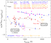 |
Fig. 5 Ro-vibrational diagrams of absorption components of the infrared HCN lines at 7.5 and 13–14 μm. The filled blue, magenta, brown, and red dots correspond to the lines of the bands 2ν2 (σ+), 3ν2 (π) − ν2(π), 4ν2 (σ+) − 2ν2(σ+), and 4ν2 (δ) − 2ν2(δ), respectively (7.5 μm). The empty blue, magenta, and brown empty triangles represent the lines of the bands ν2 (π), 2ν2 (σ+) − ν2(π), and 2ν2 (δ) − ν2(π) at 13–14 μm. The dots related to the hot bands (except 4ν2(σ+) − 2ν2(σ+) and 4ν2 (δ) − 2ν2(δ); see text) are vertically shifted to make them coincide with the fundamental band at 13–14 μm and with thefirst overtone at 7.5 μm to get more populated data sets. An additional offset of − 2 units is added to the data at 13–14 μm to improve visibility. Four populations with various rotational temperatures derived from the fitted solid straight lines can be distinguish (cold, warm, hot, and very hot). The dashed straight line is a fit to the lines of the 4ν2 (σ+) − 2ν2(σ+) band, which implies a negative rotational temperature (see text). |

4.3 The best fit to the observed HCN lines
4.3.1 Spherically symmetric model
The fits to some of the lines obtained using the radiative transfer code can be found in Fig. 6 and the derived parameters are included in Table 2. The H13 CN lines were fitted by varying only the abundance and the photodissociation radius as no strong excitation temperature variations are expected (Fig. 7).
An initial assumption of a constant radial velocity profile equal to 8 km s−1 from the stellar photosphere and outwards (Izumiura et al. 1995; Ramstedt & Olofsson 2014), produces synthetic profiles for the 7.5 μm region narrower than those observed, considering the EXES’ spectral resolution (FWHD ≃2.5 km s−1 compared to ≃ 5.4 km s−1 for low-J lines of the overtone 2ν2(σ+)). Additionally, their absorption components peak at Doppler velocities with respect to the systemic one ≳ − 7.5 km s−1, substantially different from the observed peak velocities (≳ −4.5 km s−1). This disagreement can be resolved with a constant gas velocity gradient close to the star, which represents the acceleration of the ejected gas, followed by a constant expansion velocity of 8 km s−1 (Fig. 8, Table 2).
The fit to all the ro-vibrational lines indicates that the width at the baseline of the HCN lines of the fundamental band can be explained by strong turbulence in the vicinity of Y CVn. However, this model might be too simple as a few HCN lines at 14.0 μm show unexpected wings in the emission component that cannot be accounted neither with the terminal expansion velocity nor with local line widths due to turbulence (Figs. 6 and 8). Furthermore, none of these HCN lines are overlapped with sufficiently strong acetylene features.
The optically thick pure rotational lines v = 0 J = 3−2 of HCN and H13CN also show red-shifted high velocity wings (Fig. 3). Our current spherically symmetric envelope model cannot reproduce these wings, even considering the hyperfine structure, which broadens the lines at the baseline. We give a possible solution to this problem in Sect. 4.3.2.
The best fit to the HCN lines at 7.5 μm is compatible with a constant profile for the abundance with respect to H2 in the gas acceleration region (r ≃ 1–30R⋆). However, the vibrationally excited lines at 13–14 μm cannot be fitted with such an abundance distribution and, instead, an abundance at the stellar photosphere lower by a factor of ≃ 4 is needed. The lines at 7.5 μm indicate that HCN is in rotational LTE close tothe photosphere but Trot is steeper than TK moving outwards. The 13–14 μm lines suggest that HCN may be out of rotational LTE even close to the stellar photosphere (see Fig. 9).
Cold and warm gas is strongly involved in the formation of the pure rotational lines v = 0 J = 3−2 of HCN and H13 CN. These lines cannot be accurately reproduced, which means that our model is also too simple for the outer envelope (Fig. 3). However, our synthetic lines partially fit the profiles of the observed data. Their intensities are compatible with a constant abundance with respect to H2 of ≃ 1.3 × 10⁻⁴ and an isotopic ratio 12C/13C ≃2.5 throughout the whole envelope, which is valid also for the mid-IR spectra.
The red-shifted side of the v = 0 J = 3−2 rotational HCN line can be fitted assuming that the abundance and excitation temperatures derived from the ro-vibrational lines in the mid-IR hold throughout the whole CSE, and if the HCN photodissociation shell is located at ≃170R⋆ (≃ 1′′.2) from the star. The rotational temperature at this distance from the star drops down to ≃ 85–90 K. Our envelope model cannot describe the blue-shifted part of this line as the self-absorption mentioned above is not strong enough. The results derived for H13 CN are compatible with a photodissociation region placed about 15R⋆ closer to thestar (Table 2).
The fit to the v = 0 J = 1−0 HCN line requiresmaser emission to reproduce the observed central peak in addition to the red-shifted narrow spike that the line shows at ≃ + 4 km s−1. Thermal emission is only noticeable in the wings of this line and the rest is dominated by maser emission (Dinh-V-Trung & Nguyen-Q-Rieu 2000). The H13CN v = 0 J = 1−0 line is very similar and most of it has to be explained by maser emission as well.
In summary, we did not find a spherically symmetric envelope model able to simultaneously reproduce all the observations (7.5 μm, 13–14 μm, and mm range – see Fig. 6). Thus, we propose an asymmetric envelope model in the next the section that roughly describes most of the observed lines.
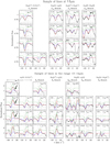 |
Fig. 6 Sample of observed HCN lines in the mid-IR (black histogram) with their best fits (spherically symmetric models; red curves) grouped in bands. The blue solid lines in the range 13–14 μm were calculated with the spherically symmetric envelope model that better fits the lines at 7.5 μm and vice versa (see Table 2 and text). The green solid lines were calculated with the asymmetric envelope model (see Sect. 4.3.2). They are vertically shifted to improve the visibility. The gray curves are the atmospheric transmission. The black arrows point at possible red-shifted wings. The vertical dashed-dotted and dashed lines are the systemic velocity (0 km s−1) and the terminal Doppler velocities derived in this work (≃8 km s−1), respectively. All the fits are reasonably good except those to the lines of band 2ν2 (δ) − ν2(π), Q branch (see text). |
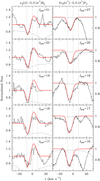 |
Fig. 7 Sample of observed H13CN lines in the mid-IR (black histogram) with their best fits (spherically symmetric models; red curves) grouped in bands. The gray curves are the atmospheric transmission. The vertical dashed-dotted and dashed lines are the systemic velocity (0 km s−1) and the terminal Doppler velocities derived in this work (≃8 km s−1), respectively. |
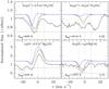 |
Fig. 8 Effect of varying the turbulent velocity and the gas expansion velocity at the stellar surface (green and blue, respectively) on the synthetic profiles coming from different regions of the envelope. The observations are the black histograms and the best fits are plotted in red. In the green curves, the turbulent velocity was set to 5 km s−1. The blue curves were calculated with a constant gas expansion velocity of 8 km s−1 throughout the whole envelope. These curves are vertically shifted for clarity. Elow is the energy of the lower level of the ro-vibrational transitions. The gray solid curves are the atmospheric transmission. The vertical gray dotted-dashed and dashed lines indicate the systemic velocity and the Doppler shifts related to the terminal velocity. |
 |
Fig. 9 Temperatures involved in the envelope models. The kinetic temperature, TK, was adopted from Guélin et al. (2018). The rotational and vibrational temperatures, Trot and Tvib, were derived in this work (Table 2). The shaded regions are the 1σ errors. The uncertainties of the vibrational temperatures are not plotted for the sake of clarity. The temperatures with the same symbol(† or ‡) coincide. |
 |
Fig. 10 H2 density, HCN abundance with respect to H2, rotational temperature in the vibrational ground state, and gas expansion velocity projected onto the line of sight derived from the asymmetric envelope model. The abscissas are the depth across the envelope measured from the closer position to Earth backwards. The ordinates are the position in the plane of the sky along an undetermined direction since the 2D envelope model shows cylindrical symmetry around the line of sight. Each quantity is plotted twice, at large scale (left) and at small scale (right). In the maps to the left, the yellow dotted-dashed and dashed circles represent the HCN dissociation radii derived in this work for the spherically symmetric envelope model (Rph = 168R⋆) and for the asymmetric model that accounts for the self-absorption in the pure rotational lines (Rph = 380R⋆), respectively (see text). In the maps to the right, the filled orange circle is the central star. |
4.3.2 Asymmetric model
A multidimensional approach involving at least 2D asymmetries seems necessary to find a more realistic envelope model that explains all the features simultaneously. Nevertheless, this model is a rough approximation and aims to provide some qualitative clues about the actual CSE of Y CVn.
Most of the inner envelope characteristics were reasonably well described by the spherically symmetric model derived from the analysis of the lines at 13–14 μm. The spherically symmetric model derived from the lines at 7.5 μm, with slight modifications, was used to describe the conical region in front of the star with the star at its apex, its axis parallel to the line of sight, and an aperture of 30°. The addition of shells with different physical and chemical conditions beyond the photodissociation radius for the spherically symmetric model allowed us to describe the pure rotational lines, in particular the blue-shifted self-absorption components and the red-shifted wings of the v = 0 J = 3−2 lines. Figure 10 contains maps of the H2 density, the HCN abundance with respect to H2, the rotational temperature of HCN, and the gas expansion velocity projected along the line of sight.
The wings observed in the J = 3−2 rotational lines (Fig. 3) are reproduced after increasing the gas expansion velocity in the region 125–200R⋆ to ≃ 9−10 km s−1 along the line of sight in the CSE hemisphere behind the star. We stress that these wings cannot be explained by the hyperfine structure of HCN (and H13CN).
The formation of the self-absorptions is mostly related to gas expanding at velocities as low as 4.5 km s−1. They can be roughly replicated by adding cold HCN in the region of the CSE corresponding to the hemisphere facing us that expands obliquely with an inclination with respect to the plane of the sky greater than 10° beyond ≃ 200R⋆. In this region of the envelope, the required rotational temperature ranges from 5 to 15 K.
The new photodissociation radius (≃380R⋆), the uncertainty of which is as least as high as the line flux calibration errors (≃ 20%), suggests that there could be cold HCN in the outer envelope that does not significantly contribute to the emission of the v = 0 J = 3−2 lines as the bulk of them come from the region of the CSE inwards from ≃ 170R⋆. The HCN column density in front of the star calculated with this model is ≃ 3.5 × 1018 cm−2.
The comparison of the observed lines and those produced by our spherically symmetric and asymmetric models (red and blue in Fig. 3) confirms our assessment about which rotational lines show maser emission (Sect. 4.2). The emissions of the HCN and H13CN lines v = 0 J = 1−0 as well as the HCN lines  J = 3−2 and
  J = 3−2 are essentially of maser nature. All these masers can be roughly reproduced by adding a few compact maser emitting regions preferentially located at the stellar photosphere and at the end of the acceleration region. In the latter shell, the gas density and its expansion velocity are high enough to produce maser peaks at any Doppler velocity in the millimeter spectrum, depending on the expansion direction. The maser contributions produced by our model are usually narrower than the observed ones but we think that they can be described if the maser emitting region is radially more extended than we assumed, it covers a larger part of the gas acceleration zone, or it comprises different isolated emitting shells or arcs.
5 Discussion
5.1 The continuum emission
5.1.1 The effective temperature of Y CVn
The effective temperature derived from our analysis is 2910 ± 70 K. This value is higher than the effective temperature of 2860 K reported by Ohnaka et al. (1999) and 2760 K proposed by Bergeat et al. (2001), which was reinforced by De Beck et al. (2010). Goebel et al. (1980) determined that the effective temperature ranges from 2750 to 2900 K from a series of infrared observations taken over two years. All these measures differ by 150 K or less suggesting that the disagreement is only apparent and it is likely produced by observational uncertainties and stellar pulsation effects.
However, our estimate is not compatible with the effective temperatures assumed or derived by others (e.g., Teyssier et al. 2006; Schöier et al. 2013; Ramstedt & Olofsson 2014), which are more than 25% lower. These results are based on photometric observationsin the J (1.25 μm) to M (4.8 μm) bands. These measurements are going to be possibly confused by effect of the strong molecular bands of CO, C2, C3, C2 H2, CN, and HCN that exist below 5 μm.
5.1.2 Dust grains composition and distribution throughout the CSE
One of the most interesting results of our fit is the absence of amorphous carbon close to the star, contrary to what occursin IRC+10216. In the latter, the bulk of the carbonaceous material condenses onto the dust grains at ≃ 5R⋆ from the center of the star (Fonfría et al. 2008), where the gas kinetic temperature is ≃ 800−1000 K. This condensation temperature is reached in Y CVn in the shell that extends from 4.9R⋆ to 6.8R⋆, where the gas density is ≃ 1–2 × 107 cm−3. However, the ISO observations indicate that most of the AC emission comes from a region of the CSE where the gas kinetic temperature is below 100 K. The gas in this region is rarefied (gas density ~ 104 cm−3, typical of dense molecular clouds), highly decreasing the depletion rate of any possible refractory molecular species that could produce the AC in the grains and, thus, increasing the grain growth timescale beyond ~ 1 Myr (Hirashita 2000). This timescale is too long compared to the typical kinetic times involved in the evolution of AGB CSEs (~ 100–1000 yr). The low kinetic temperature comes with an increase in the density of dust grains by a factor of 15 in order to reproduce the observed flux densities, which can also be explained as an increase of the grain size by a factor of ≃ 2.5, if we assume optically thin grains.
This result can be explained if the condensation of the refractory carbon-bearing molecules onto the SiC dust grains which form AC close to the star stopped in the past and the AC we are seeing is the remnant of this process. It would have ended about 200–300 yr ago, if we assume an expansion velocity for the dust grains twice as high as the terminal gas expansion velocity of ≃ 8 km s−1. A dusty shell like this, which we place at ≃1′′.5 from the star, should not be confused with the detached shell found by Young et al. (1993) and Izumiura et al. (1996), which is located at ≃ 180′′–190′′ from the star. Thus, we could consider that these kind of dusty shells might be formed periodically or, at least, that the latter was not formed by an unique event.
5.2 Considerations of the molecular envelope model
5.2.1 The gas expansion velocity
The gas expansion velocity profile derived during our analysis is in good agreement with a typical profile produced by gas acceleration by radiation pressure on dust grains (e.g., Goldreich & Scoville 1976; Bowen 1988; Decin et al. 2006). The gas accelerates from a low velocity roughly at the photosphere over a zone of a few stellar radii to reach a terminal velocity similar to previously reported values derived from pure rotational lines (Izumiura et al. 1995; Ramstedt & Olofsson 2014; Massalkhi et al. 2018b). The condensation of SiC seems to be responsible for the gas acceleration.
However, this gas expansion velocity field cannot satisfactorily explain the red-shifted wings found in the Q branch mid-IR lines of the HCN band ν2(π) (see Sect. 4.3.1 and Fig. 6). These wings are not present in high-J lines and they are not expected to be noticeable in many other lines of this band due to the high line density of the observed spectral ranges. They could mean that the gas responsible, which would be located at a few tens of R⋆, is expanding faster than the terminal velocity.
Moreover, the J = 3−2 lines in the vibrational ground stateof HCN and H13CN display evidence of a higher gas expansion velocity (Fig. 3). These lines are optically thick and only anincomplete shell with gas expanding faster than the terminal velocity and located in the outer envelope can explain this effect. We note that the need for an incomplete shell cannot be a consequence of an exceedingly narrow telescope main beam since the HCN emitting region of the envelope is completely covered by it (2Rph(HCN) ≃ 380R⋆ ≃ 5′′.3 and the half power beam width,HPBW(266 GHz) ≃ 9′′.2). Thus, both the IR and the mm lines could be tracing gas placed between a few tens of stellar radii and ≃ 200R⋆, expanding at up to ≃ 10 km s−1. This velocity could be higher if the gas expands along a direction different from the line of sight.
5.2.2 The turbulent velocity
The fits to the mid-IR lines suggest that close to the photosphere the local line width of the HCN lines is ≃ 10 km s−1. The thermal broadening for HCN, at the kinetic temperature prevailing near the photosphere of Y CVn, is ≃ 1 km s−1. Considering a Maxwell-Boltzmann velocity distribution, the gas turbulent velocity is therefore as high as ≃ 6 km s−1.
For IRC+10216, many lines coming from the vicinity of the photosphere, which have a line width ranging from 5 to 8 km s−1, have been found so far (Patel et al. 2009; Cernicharo et al. 2011; Velilla Prieto et al. 2015). These line widths represent turbulent velocities of ≃ 3−5 km s−1 (Monnier et al. 2000), which are considered to be related to strong turbulence typical of the innermost layers of the envelope of an AGB star, where efficient matter ejection mechanisms are enabled.
Hence, the comparison between the turbulent velocity for Y CVn and IRC+10216 suggests that (1) unexpectedly violent mechanisms at work close to the photosphere of Y CVn produce very strong turbulence, (2) the turbulent velocity close to the photosphere of IRC+10216 is underestimated, or (3) the line width of the HCN lines observed in Y CVn is produced by turbulence along with other gas acceleration mechanisms not included in our model. This latter scenario is based on the fact that the lack of spatial resolution could lead us to confuse turbulence in the circumstellar envelope with other photospheric phenomena such as higher velocity gas ejections, convective cells, or the pulsating movement of the photosphere (Freytag et al. 2017). The high Doppler shifts and full widths at half maximum (FWHMs) of atomic lines that were observed in red supergiants and Miras for some time (e.g., Smith et al. 1989; Hinkle et al. 2002; Gray 2008; Stothers 2010) would support the existence of these phenomena.
5.2.3 HCN abundance with respect to H2 and column density
The fits to all the data are compatible with an HCN abundance of ≃ 1.3 × 10⁻⁴ throughout most of the envelope with an anomaly very close to the photosphere that implies a decay of the abundance down to 3.5 × 10⁻⁵. The error for this quantity in the inner envelope is better than 10% due to the redundancy provided by the high number of observed vibrationally excited lines that come from the vicinity of the star. The impossibility of determining the thermal emission of the HCN v = 0 J = 1−0 line and the calibration errors of the pure rotational lines lead us to think that a factor of 2 for the abundance in the outer envelope could be a better estimate than the one based on the sensitivity of our model to the free parameters (≃ 15%; Table 2). An additional uncertainty related to the determination of the distance to Y CVn has to be considered. In the current work we adopted the distance published in the Gaia EDR3 (310 ± 17 pc; Gaia Collaboration 2021) but shorter distances were proposed before (≃ 220 pc (Abia & Isern 2000; Schöier et al. 2013)and 232 ± 13 pc (Gaia DataRelease 2; Gaia Collaboration 2018)). Consequently, the HCN and H13 CN abundances might be 30% lower than we propose.
This abundance profile is based on a gas density ∝ r−2 beyond the photosphere but this profile could be steeper in the region between the photosphere and r ≃ 2–3R⋆ (e.g., Agúndez et al. 2020, and references therein). The adoption of a gas density profile like this would reduce the HCN abundance close to the star with respect to that over the rest of the CSE even more as the HCN column density has to be the same to reproduce the observations. Therefore, the abundance for this region of the CSE derived in this work has to be taken as an upper limit.
The average column density for HCN that we derived from our fits (see Table 2) is (2.1 ± 1.1) × 1018 cm−2 and we proposed in Sect. 4.2 an upper limit of ≃ 5.1 × 1018 cm−2 under vibrational LTE. However, the detailed analysis of the lines makes clear that HCN is always vibrationally out of LTE (see Sect. 4.3 and Fig. 9). More precisely, the vibrational partition function derived from our best fits to the mid-IR lines is below ≃ 4.2 (it is below ≃ 19 under vibrational LTE; Sect. 4.3). Thus, the HCN column density derived from the ro-vibrational diagram considering the vibrational temperatures obtained from the modeling process is (1.2 ± 0.3) × 1018 cm−2, fully compatible with the result of our fits.
An observational estimate of the HCN abundance in the inner layers of the envelope of Y CVn has not been reported to date (as far as we know in the literature) but the photospheric abundance was determined to be 1.9 × 10⁻⁵ by Olofsson et al. (1993b). This abundance is the value in the upper layers of a static LTE model atmosphere which reproduced the results of Lambert et al. (1986). It is compatible with the value that we derived from the analysis of the observations in the 13–14 μm range but it is 7 times lower than the one inferred from the spectrum at 7.5 μm. This disagreement can be explained by asymmetries or clumpiness around the star, which would reduce the HCN column density without diminishing its abundance, or by the gas phase chemistry in the vicinity of the star, where the HCN abundance could be significantly lower than in the rest of the envelope (e.g., Fonfría et al. 2008; Agúndez et al. 2020).
The rest of the abundance estimates in the literature were derived apparently from the analysis of the v = 0 HCN lines J = 1−0, 3− 2, and 4− 3. Olofsson et al. (1993b) reported an HCN abundance with respect to H2 that follows a Gaussian profile with a value at the stellar photosphere of 8.3 × 10⁻⁴ and a photodissociation radius of 1.2 × 1015 cm (≃ 50R⋆ for us). The average abundance is ≃7.3 × 10⁻⁴, that is about 6 times higher than ours. This disagreement can be due to three reasons: (1) they used only the HCN v = 0 J = 1−0, which shows maser emission (e.g., Dinh-V-Trung & Nguyen-Q-Rieu 2000), (2) their photodissociation radius is very small compared with ours (≃ 170–380R⋆), and (3) the different distance from the star and mass-loss rate that these authors used (D ≃ 290 pc and Ṁ ≃ 4–6 × 10⁻⁸ M⊙ yr−1; Olofsson et al. 1993a).
Bachiller et al. (1997) gave an average CN abundance with respect to H2 of 7.9 × 10⁻⁵ in a shell spanning from 20 to 200R⋆ with the parameters considered in the current work. Since CN is a direct photodissociation product of HCN, this abundance can be taken as a lower limit for the HCN abundance, which is in good agreement with our results. Lindqvist et al. (2000) found that the CN abundance distribution with respect to that of H2 peaks at 5.5 × 1015 cm from the star, that is ≃170R⋆ (using the distance and stellar radius given in Table 1). They gave an HCN abundance greater than 6 × 10⁻⁵ also compatible with the abundance estimated in the current work.
Schöier et al. (2013) gave an abundance with respect to H2 at the star of 3.0 × 10⁻⁵ and a photodissociation radius of 1.0 × 1016 cm (≃ 430R⋆ with the angular stellar radius that we adopted and the distance to the star that they chose, that is ≃ 220 pc). The average abundance is thus 2.7 × 10⁻⁵. Their maximum and average abundances are about a factor of 5 lower than ours, which make our abundance a priori incompatible with theirs. However, the authors estimate the uncertainty of their abundance to be of a factor of 3. This uncertainty along with the one derived for the outer CSE in the current work (≃ 50%; Table 2), the different distances to the star adopted in both works, and the calibration errors related to the millimeter observations could make both results more compatible.
As we noted in Sect. 4.2, the HCN column density in the CSE of Y CVn is surprisingly high compared to that in IRC+10216 (≃ 2.1 × 10¹⁸ and 1.6 × 1019 cm−3, respectively; Fonfría et al. 2008), considering the high disparity between their mass-loss rates (≃ 1.4 × 10⁻⁷ and 2.7 × 10⁻⁵ M⊙ yr−1; Guélin et al. 2018). This fact is even clearer when their HCN abundances with respect to H2 are compared: they are ≃1.3 × 10⁻⁴ in the envelope of Y CVn and 0.6–2.4 × 10⁻⁵ in IRC+10216, if we correct the abundance derived by Fonfría et al. (2008) for a distance of 120 pc (Groenewegen et al. 2012) and the mass-loss rate of Guélin et al. (2018). Hence, the HCN abundance in the envelope of Y CVn is one order of magnitude higher than in IRC+10216, the archetypal C-rich AGB (N-type) star. Nevertheless, this can be explained if we consider that the HCN abundance grows from its photospheric value as the distance from the star increases while the CN abundance steeply decreases (Agúndez et al. 2020). The column density of photospheric CN in Y CVn is at least as high as in IRC+10216 (e.g., Barnbaum 1994; Bakker et al. 1997; Fonfría et al., in prep.) but the H2 column density in the envelopes of these stars are substantially different.
5.2.4 The 12C/13C isotopic ratio
The fits to the HCN and H13CN lines that we have done in this work confirms once more (Lambert et al. 1986; Olofsson et al. 1993b; Ohnaka et al. 1999; Schöier & Olofsson 2000; Milam et al. 2009; Ramstedt & Olofsson 2014; Abia et al. 2017) that the isotopic ratio 12C/13C in the envelope of Y CVn is typical of a J-type star. Our result of 2.5 is in good agreement with the previous estimates, which range from 2 to 8. Moreover, the two isotopic ratios that we derive for the inner and outer envelope suggest that this quantity has not substantially changed over the last 350 yr.
5.2.5 The extent of the HCN and abundance distribution
The photodissociation radius obtained in the current work ranges from ≃ 170 to 380R⋆. It is contained within the domain determined from prior observational estimates (50–420R⋆). Yet, the data dispersion of the measures is too high and the agreement between these measures poor.
The CN(1−0) interferometer observations analyzed by Lindqvist et al. (2000) indicate that the HCN abundance distribution, which has to be smaller than the CN abundance distribution, cannot extend further than ≃ 430R⋆ from Y CVn (using the distance to the star and stellar radius of Table 1, and assuming a roughly spherically symmetric photodissociation shell). In fact, the HCN abundance distribution is likely limited to within 200R⋆ from the star, that is, inside the CN abundance peak. However, the CN brightness distribution integrated over velocity is elongated along the north-south direction and it consists of several bright spots at the systemic velocity, which suggests that the outer envelope of Y CVn can be irregular or clumpy.
In any case, our result is in better agreement with the largest photodissociation radius proposed by Schöier et al. (2013), ≃ 430R⋆, and with the radius of the region that contains the CN emission (Lindqvist et al. 2000) than with the rest of the estimates. Nevertheless, the use of Eq. (7) of Massalkhi et al. (2018b) and the interstellar photodissociation rates for HCN in Table B.1 of Agúndez et al. (2018) gives that the HCN abundance decreases by a factor of 10 with respect to its photospheric value at ≃ 75R⋆. This radius is compatible with the shortest observational estimates.
This disagreement might indicate that either the interstellar UV radiation field is actually weaker around Y CVn’s location in the Galaxy, or there is a dust shell optically thicker than expected that protects the HCN inside. The latter scenario might be related to the increased density of dust grains that we propose to exist beyond ≃ 200R⋆ (Sect. 4.1).
5.2.6 The kinetic, rotational, and vibrational temperatures
In this work, we adopted the kinetic temperature dependence over the outer layers of the envelope of IRC+10216 for the CSE of Y CVn based on their similar chemical composition and low gas density (Sect. 3.1). We note however that the properties of the dust grains (such as size and expansion velocity) in both environments are different due to the particular physical and chemical conditions in their dust formation zones. Hence, a detailed modeling of the thermal balance (e.g., Decin et al. 2006), which is out of the scope of the current work, may conclude that the kinetic temperature profile in Y CVn is different than assumed.
It can be argued that such a difference could significantly influence our results. Nevertheless, the code that we used relies on input excitation temperatures which are implemented to be independent of the kinetic temperature (Appendix C). Consequently, TK is only usedas the excitation temperature by default and to calculate the thermal line width. Our results indicate that the local line width is dominated by turbulence and the number of modeled lines is high enoughto allow us to estimate the rotational and most of the vibrational temperatures. Only a few Tvib were considered as equal to TK in the best fit model and all of them describe the population relation between adjacent vibrational states whose energy difference is only of a few tens of K (e.g., 2ν2(σ+) and 2ν2 (δ); Table 2), that is much smaller than the typical TK in the region of the CSE where these vibrational states are populated. Therefore, the effect of a change of TK on our results is quite limited and can be neglected.
The rotational temperatures near the photosphere derived from the fits to the lines at 7.5 and 13–14 μm differ by more than a factor of 2 between them (Fig. 9). In contrast, the Trot profiles beyond Rii ≃ 3.2R⋆ are quite similar (see Table 2) and can be assumed to be the same ( K). The low rotational temperature in the acceleration zone (r ≃ 1.0–3.2R⋆) that affects the lines observed at 13–14 μm implies that there is a substantial emission deficit in the high-J lines formed in this shell. The gas density in this region is ~ 108–1010 cm−3, high enough to roughly thermalize the rotational levels of HCN by collisions with H2. Hence, this low Trot may be explained by a clumpy or incomplete emitting shell in terms of the gas density or HCN abundance, an explanation already invoked by Dinh-V-Trung & Nguyen-Q-Rieu (2000) and compatible with our findings about the decrease of the HCN abundance close to the star. In this scenario, the emission component of the high-J lines would be more affected than those of the low-J ones, which are essentially formed further from the star.
Most of the vibrational temperatures are ≲ 1500 K, far below the effective stellar temperature (≃2900 K). However, the vibrational temperatures are biased by the bulk emission and absorption of the high excitation HCN lines located ≃ 1R⋆ beyond the photosphere. The vibrational temperature across this shell can decrease very fast due to the typically high Einstein coefficients of the HCN ro-vibrational levels (Aul ≃ 0.5–5 s−1) making our result compatible with HCN under vibrational LTE at the photosphere.
Either way, our results indicate that the vibrational states are predominantly radiatively excited throughout most of the envelope in good agreement with the fact that the critical density for the ro-vibrational transitions (with de-exciting collisional rates usually below 10−10 cm3 s−1; e.g., González-Alfonso et al. 2002; Toboła et al. 2008) is higher than at any region of the envelope (ncrit ≳ 1010 cm−3). This critical density is typically of 10–100 times higher than for the pure rotational lines, which explains the excitation differences between the rotational and vibrational temperatures.
Among the vibrational temperatures derived from our fitting process there is one clearly incompatible with the rest. The Tvib[2ν2(δ) − 2ν2(σ+)] as derived from the 7.5 μm lines is compatible with the kinetic temperature (≃ 2900−1300 K for r = 1.0–3.2R⋆), which is as expected for two vibrational states so close in energy (ΔEvib ≃ 30 K). However, the Tvib derived from the 13–14 μm is much lower (≲50 K). Figure 6 shows how the model systematically overestimates the absorption of the lines of the Q branch of the 2ν2 (δ) − ν2(π) band by a factor of up to 2 while the lines of the R and P branches are satisfactorily well reproduced. This is not physically possible as the lines of these three branches involve the same ro-vibrational levels. Moreover, the code has been thoroughly tested over the years and the lines of the three branches are calculated simultaneously with the same formulas. This disagreement can be a consequence of inaccurate Einstein coefficients for the lines of the R or Q branches of the 2ν2(δ) − ν2(π) band, as we suggested during the analysis of the ro-vibrational diagram (Sect. 4.2), but also the effect of radiative transfer mechanisms not considered in the envelope model, such as maser emission in high-J lines or initially unexpected emission and absorption effects due to high line optical depths (e.g., Lacy 2013). Moreover, the ro-vibrational lines of the 4ν2(σ+) − 2ν2(σ+) band might be affected by the Fermi resonance that exists between the vibrational states ν2 + ν3(π) and 4ν2(σ+), which causes strong maser emission in the lines of the latter state and was detected in Y CVn by Schilke & Menten (2003).
5.2.7 Maser emission in the vibrational ground state and ν2
Dinh-V-Trung & Nguyen-Q-Rieu (2000) did a deep analysis of the maser emission of the HCN line v = 0 J = 1−0 roughly explaining the overall line profile except for the central peak. The pumping mechanism mostly relies on the vibrational excitation produced by photons involving the ν1 (σ+)3 band at 3 μm, where the stellar radiation field is strong (see Fig. 4).
Most of the bumps in the line profile were explained as blue- and red-shifted maser peaks related to each component of the hyperfine structure if the gas expansion velocity were 6 km s−1. This velocity is in good agreement with our conclusion that the maser emission is mostly produced at the end of the acceleration region. The Doppler velocity of the red-shifted spike at +5 km s−1 with respect to the central peak of the line has not changed significantly in 20 yr, which suggests that the gas acceleration mechanism has been stable during the last decades. On the contrary, the intensities of several of these peaks do change over time, as it can be seen when the observation by Dinh-V-Trung & Nguyen-Q-Rieu is compared with those by Schöier et al. (2013) and ours. These variations may be related to the stellar pulsation period or they may indicate a change of the physical conditions in the maser pumping region due to the evolution of the ejected matter, which is fully accelerated in about 5 yr. The rest of the HCN v = 0 J = 1−0 line shows broadcomponents overlapped rather than spikes. This is evidence of an extended maser emitting region comprising different expansion velocities, where the radiation is likely enhanced due to the high turbulent velocity prevailing in the acceleration zone (Sect. 5.2.2). In this scenario, the central peak is very likely produced at the stellar photosphere.
The HCN line  J = 3−2 is undoubtedly a maser from an inspection of its profile: displaying two narrow peaks, and its intensity, which is almost as high as the line J = 3−2 of the vibrational ground state. Its comparison with the same line of H13CN supports this conclusion as the HCN one is 150 times stronger even though it should be similar to the isotopic ratio 12C/13C ≃ 2.5, had both lines a thermal origin. The HCN line
  J = 3−2 is about 15 times stronger than the corresponding H13CN line, also stronger than expected. Therefore, the HCN f line could be a weak maser as well.
Contrary to what occurs in IRC+10216, where the  J = 2−1 maser is favored by the strong continuum emission at 7 and 14 μm (Lucas & Cernicharo 1989; Menten et al. 2018), the
  J = 3−2 maser in Y CVn is probably pumped by the continuum emission at 3 μm, as the continuum is significantly weaker at longer wavelengths (Fig. 4). The hot band ν1 + ν2(π) − ν2(π), which is as strong as ν1 (σ+), along with the fact that molecules in the ro-vibrational level
  J = 1 can be de-excited to the vibrational ground state, could result in population inversion. This pumping mechanism is compatible with possible maser emission in the
  J = 2−1 line, which was not observed in Y CVn.
5.2.8 Reliability of the spatial asymmetries in the abundance distribution and gas expansion velocity field
The existence of asymmetries in the inner layers of the CSE comes from the incompatibilities found in the physical and chemical conditions derived from the mid-IR spectra of HCN. The observations at 7.5 and 14.0 μm were acquired with the same instrument (SOFIA-EXES) under very similar conditions and along two consecutive nights. The data at 13.1 μm were taken with IRTF-TEXES about two months prior. In principle, it might be possible to find incompatibilities between the IRTF-TEXES data at 13.1 μm and the SOFIA-EXES data at 14.0 μm due to instrumental differences or effects related to the stellar pulsation phase but the results turned out to be highly compatible. Nevertheless, the data sets acquired with SOFIA-EXES almost simultaneously are those that display the largest incompatibilities. This suggests that the disagreements that we find are very likely real. In fact, Ragland et al. (2006) warned about the possible existence of asymmetries in the innermost envelope of this star.
At larger distances from the star, the velocity field of the expanding gas and the HCN abundance distribution might be asymmetric as well. The lack of other purely thermal rotational lines in our study in addition to the HCN and H13 CN v = 0 J = 3−2 ones brings some uncertainties in the determination of the physical conditions throughout the outer layers of the envelope and the photodissociation radius. However, there is no reason to think that the red-shifted wing found in these lines is related to any instrumental issue or error during the observation process. It can be argued that these wings are actually the hyperfine components with the lowest frequencies but, in this case, it is not possible to reproduce the observed profiles unless the red-shifted part of the lines are partially absorbed, something that would require an unlikely rotational temperature profile behind the star.
6 Summary and conclusions
We present new single-dish high spectral resolution observations of the AGB star Y CVn in the mid-IR ranges 7.35–7.60, 13.00–13.25, and 13.93–14.04 μm acquired with SOFIA-EXES and IRTF-TEXES. We identified about 130 lines of HCN and H13 CN of the bands ν2(π), 2ν2 (σ+), 2ν2 (σ+) − ν2(π), 2ν2 (δ) − ν2(π), 3ν2 (π) − ν2(π), 3ν2 (π) − 2ν2(σ+), 3ν2 (π) − 2ν2(δ), 3ν2 (ϕ) − 2ν2(δ), 4ν2 (σ+) − 2ν2(σ+), and 4ν2 (δ) − 2ν2(δ), which display either P Cygni or pure absorption profiles. These data sets were complemented with the pure rotational lines J = 1−0 and 3− 2 in several vibrational states, which were observed with the IRAM 30 m telescope at 1.12 and 3.38 mm, and the continuum emission taken with ISO.
We analyzed the HCN and H13CN lines following two different approaches: (1) an overall study based on a ro-vibrational diagram, and (2) a detailed analysis in 1D and 2D thatmakes use of a code that reproduces the molecular and dust absorption and emission of the envelope of an AGB star (Fonfría et al. 2008, 2014). The results derived from these analyses lead us to conclude that:
The continuum emission can be described by a central star with an effective temperature of ≃2900 K and an optically thin dusty cocoon. The dust grains are mostly made of SiC in the inner layers of the envelope and of AC in the outer envelope. The bulk of SiC condenses at ≃3.0–3.5R⋆ from the center of the star and the AC beyond ≃200R⋆. At this distance, the density of dust grains seems to be about 15 times higher than predicted for a dusty isotropically expanding CSE.
The detailed modeling to the observed data and the ro-vibrational diagram suggest the existence of asymmetries in the physical and chemical conditions throughout the envelope.
The line profiles are compatible with a radial gas expansion velocity profile growing from ≃0.5 up to ≃8 km s−1 in the first 2R⋆ beyond the photosphere. The terminal expansion velocity that we use in our models ranges from 6 to 10 km s−1 along different directions but the actual maximum velocity might be even higher. These variations might be related to higher velocity outflows.
The observed mid-IR lines are broader than expected. The best fits were achieved with a line width at the stellar photosphere of ≃10 km s−1, that implies a turbulent velocity of ≃6 km s−1. Such a high turbulent velocity might be hiding other phenomena as high velocity matter ejections or photospheric movements related to the stellar pulsation or convection.
The HCN abundance with respect to H2 is ≃1.3 × 10⁻⁴ throughout most of the envelope. The abundance may be significantly lower in the vicinity of Y CVn. The average column density is ≃2.1–3.5 × 1018 cm−2, only one order of magnitude lower than for IRC+10216.
The rotational and vibrational temperatures of HCN are out of LTE throughout most of the envelope, which suggests that the collisions are too scarce to thermalize the gas even rotationally.
The pure rotational lines v = 0 J = 1−0 of HCN and H13CN display maser emission (e.g., Dinh-V-Trung & Nguyen-Q-Rieu 2000). The
 J = 3−2 line was found to show also evident maser emission. The
  J = 3−2 line might be a weak maser as well.
The isotopic ratio 12C/13C is determined to be around 2.5 throughout the whole envelope in good agreement with previous measures.
All these conclusions lead us to think that Y CVn is a quite active star that could have developed structure in its envelope. Due to the physical mechanisms that are producing the suggested asymmetries close to the star, the high temperatures, gas densities below ~ 108–1010 cm−3, the influence of the Galactic UV radiation field in the chemistry at different distances from the star, and its proximity, Y CVn is a good candidate to better understand the physical and chemical evolution of the envelopes of low mass-loss rate C-rich stars.
Acknowledgements
We thank the anonymous referee for their accurate and helpful comments provided during the reviewing of this manuscript. The research leading to these results has received funding support from the European Research Council under the European Union’s Seventh Framework Program (FP/2007–2013)/ERC Grant Agreement no. 610256 NANOCOSMOS. EJM acknowledges financial support for this work through award #06_0144 which was issued by USRA and provided by NASA. M.J.R. and EXES observations are supported by NASA cooperative agreement 80NSSC19K1701. M.S.G. thanks Spanish MCIN through grant AYA2016-78994-P. Based in part on observations made with the NASA/DLR Stratospheric Observatory for Infrared Astronomy (SOFIA). SOFIA is jointly operated by the Universities Space Research Association, Inc. (USRA), under NASA contract NNA17BF53C, and the Deutsches SOFIA Institut (DSI) under DLR contract 50 OK 0901 to the University of Stuttgart. Visiting Astronomer at the Infrared Telescope Facility, which is operated by the University of Hawaii under contract NNH14CK55B with the National Aeronautics and Space Administration. This work is based on observations carried out under project numbers 155-16 and 048-17 with the IRAM 30 m telescope. IRAM is supportedby INSU/CNRS (France), MPG (Germany) and IGN (Spain). This publication makes use of data products from the Two Micron All Sky Survey, which is a joint project of the University of Massachusetts and the Infrared Processing and Analysis Center/California Institute of Technology, funded by the National Aeronautics and Space Administration and the National Science Foundation. This publication makes use of data products from the Wide-field Infrared Survey Explorer, which is a joint project of the University of California, Los Angeles, and the Jet Propulsion Laboratory/California Institute of Technology, funded by the National Aeronautics and Space Administration.
Appendix A Brief description of HCN
Hydrogen cyanide is a linear triatomic molecule that belongs to the C∞ group and displays a permanent dipole moment of 2.985 D (Ebenstein & Muenter 1984). The vibration of its atoms can be described with the aid of four normal modes, two of which are degenerate and are combined into the bending mode ν2 (π). These two degenerate normal modes involve atomic oscillations out of the molecular axis that allow the molecule to spin around it. This results in the creation of a vibrational angular momentum that splits the rotational levels in sublevels with different e − f parity (Brown et al. 1975). The other two normal modes, ν1(σ+) and ν3(σ+), are stretching modes that can be essentially described as the HC–N and H–C vibrations along the molecular axis, respectively (e.g., Herzberg 1956).
 |
Fig. A.1 Vibrational energy diagram of HCN below 5000 K. The lines that connect the vibrational states represent the strongest allowed vibrational transitions. The transitions in blue lie around 13.5 μm, in red around 7.5 μm, and in orange at other wavelengths (3.0, 3.6, 4.8, and 8.2 μm, depending on the transition). Those plotted with ticker lines are detected in the spectra presented in the current work (Figs. 1 and 2). |
In the current work, we adopted two different notations commonly used in Molecular Spectroscopy and Astrophysics to label a vibrational state: v1ν1 + v2ν2 + v3ν3(ℓ±) and  , where i = 1, 2, 3. The vi is the vibrational quantum number related to the i-th normal mode, ℓ the quantum number for the vibrational angular momentum, which can be expressed with the Greek letters σ, π, δ, ϕ, γ, … for ℓ = 0, 1, 2, 3, 4, …, ± is the total parity of the molecule in this vibrational state (usually given only for the σ states), and p is the e − f parity. The v = 0 means the vibrational ground state (G.S.). The change of the rotational number in a transition is given by Bp (Jl) for the ro-vibrational lines, where Ju and Jl are the upper and lower rotational levels, respectively, B is the branch (P: ΔJ = Ju − Jl = −1, Q: ΔJ = 0, and R: ΔJ = +1), and J = Ju − Jl for the pure rotational ones. More information about the selection rules and the line intensities of linear molecules can be found, for example, in Fonfría et al. (2008). Figure A.1 contains a vibrational energy diagram for HCN to help understand the lines analyzed in the current work.
Appendix B Ro-vibrational diagrams
The absorption and emission components of a P Cygni profile can be separated by assuming that they are produced in a layer with a constant temperature and density. In this scenario, the solution of the radiation transfer equation is:
![\begin{equation*}F_{\nu}=I_{\nu,0}\textrm{e}^{-\tau_{\nu}}\Omega+S_{\nu}\left[1-\textrm{e}^{-\tau^{\prime}_{\nu}}\right]\Omega^{\prime},\end{equation*}](/articles/aa/full_html/2021/07/aa40082-20/aa40082-20-eq28.png) (B.1)
(B.1)
where Fν is the received flux, Iν,0 is the continuum emission, τν and  are the optical depths related to the absorption and emission components, respectively, and Sν is the source function that depends on the rotational and vibrational temperatures. Each optical depth is affected by a Doppler shift. The
 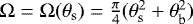 and
and  are the solid angles subtended by the absorbing and emitting regions (with sizes of θs and
  , respectively), as seen by the telescope. The angle θb is the size ofa point-like source that can be calculated by summing in quadrature the size of the Point Spread Function (PSF) of the telescope, the atmospheric seeing, and the jittering of the telescope, if present. Hence, for a normalized spectrum where the continuum flux is
 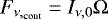 :
:
![\begin{equation*} F_{\nu}^{norm}=\frac{F_{\nu}}{F_{\nu,_{\textrm{cont}}}}=\textrm{e}^{-\tau_{\nu}}+\frac{S_{\nu}}{I_{\nu,0}}\left[1-\textrm{e}^{-\tau^{\prime}_{\nu}}\right]\frac{\Omega^{\prime}}{\Omega}.\end{equation*}](/articles/aa/full_html/2021/07/aa40082-20/aa40082-20-eq34.png) (B.2)
(B.2)
To first approximation, the optical depths can be assumed to be Gaussian-like (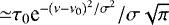 ). The simplicity of the absorption component with respect to the emission one, more affected by unknowns, leads us to use the first one to derive reliable physical and chemical quantities from our observations.
We consider the opacity of a line (e.g., Jacquemart et al. 2001; Šimečková et al. 2006):
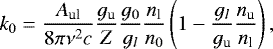 (B.3)
(B.3)
where n0 is the numerical density of molecules in the lowest energy level, nl and nu the density of molecules in the lower and upper levels involved in the transition, g0, gl, and gu are the corresponding degeneracies, and Z is the total partition function. The density fractions can be written by means of Boltzmann factors in this way:
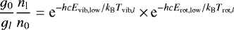 (B.4)
(B.4)
where Evib,low and Erot,low are the vibrational an rotational energies of the lower ro-vibrational level involved in the transition (Elow = Evib,low + Erot,low), Tvib,l and Trot,l (Trot, hereafter) are the vibrational and rotational temperatures for the lower ro-vibrational level, respectively, and Texc is the excitation temperature of the line.
The integral of the optical depth over the frequency, W, derived from the absorption component of the observed line4 can be related to these temperatures and the column density, Ncol, through this formula:
![\begin{align*}\ln\left[\frac{W\nu^28\pi c}{A_{\textrm{ul}}g_{\textrm{u}} N_{\textrm{col,0}}}\right]= &\left\{\ln\left[\frac{N_{\textrm{col}}}{N_{\textrm{col,0}}Z}\left(1-\textrm{e}^{-hc\nu/k_{\textrm{B}}T_{\textrm{exc}}}\right)\right]\right. \nonumber \\& \left. -\frac{hcE_{\textrm{vib,low}}}{k_{\textrm{B}}T_{\textrm{vib},l}}\right\}-\frac{hcE_{\textrm{rot,low}}}{k_{\textrm{B}}T_{\textrm{rot}}}.\end{align*}](/articles/aa/full_html/2021/07/aa40082-20/aa40082-20-eq39.png) (B.6)
(B.6)
We note that Ncol,0 is an arbitrary, constant column density introduced to produce dimensionless arguments for the logarithms.
The term 1 −e−hcν∕kBTexc can be neglected for lines in the infrared if the excitation temperature Texc ≪ hcν∕kB, as it occurs in the outer shells of the envelopes of AGB stars (Fonfría et al. 2017, 2018). However, in warmer shells its contribution can, in principle, be significant. For our data, plotted in the ro-vibrational diagram that can be seen in Fig. 5, 1 − e−hcν∕kBTexc varies less than 7% due to its dependence on the frequency. Thus, the effect of the frequency variation on the rotational temperature determination is by far much lower than the statistical noise derived from the linear fit to the scattered data sets in the ro-vibrational diagram and it can be ignored. This term can therefore be evaluated at the average frequency of each set of lines that belong to a given band,  .
.
The excitation temperature of the lines considered in this work can be expressed in terms of the vibrational and rotational temperature. For a given line with a frequency ν, considering the same rotational constant and rotational temperature for the vibrational states involved in the transition, and neglecting the contribution of the distortion and higher order rotational constants:
![\begin{equation*}\frac{hc\nu}{k_{\textrm{B}}T_{\textrm{exc}}}\simeq\frac{hc\Delta E_{\textrm{vib},\textrm{ul}}}{k_{\textrm{B}}T_{\textrm{vib},\textrm{ul}}}+\frac{hc\left\{B\left[J_u\left(J_u+1\right)-J_l\left(J_l+1\right)\right]\right\}}{k_{\textrm{B}}T_{\textrm{rot}}},\end{equation*}](/articles/aa/full_html/2021/07/aa40082-20/aa40082-20-eq41.png) (B.7)
(B.7)
where ΔEvib,ul and Tvib,ul are the energy difference and the vibrational temperature between the vibrational states involved in the transition. For the lines of the Q branch (ΔJ = Ju − Jl = 0), Texc ≃ Tvib,ul. However, for the lines of the P and R branches (ΔJ = ±1), ![$\left|B\left[J_u\left(J_u+1\right)-J_l\left(J_l+1\right)\right]\right|=2BJ_l$](/articles/aa/full_html/2021/07/aa40082-20/aa40082-20-eq42.png) and
and  , respectively. On one hand, the rotational constant of HCN is B ≃ 1.484775403 cm−1 ≃2.2 K (Maki et al. 2000) and the rotational temperature in the shells where we expect the bulk absorption of HCN to be produced is on the order of ≃ 1000 K. This means that
 ![$hc\left\{B\left[J_u\left(J_u+1\right)-J_l\left(J_l+1\right)\right]\right\}/k_{\textrm{B}}T_{\textrm{rot}}\ll 1$](/articles/aa/full_html/2021/07/aa40082-20/aa40082-20-eq44.png) . On the other hand, for the ro-vibrational lines of the HCN bands analyzed in this work (the fundamental band ν2 and the corresponding overtones and hot bands), the difference of vibrational energy between the upper and lower states is approximately a number of times the energy of the ν2 normal mode, which is ≃ 713.4610 cm−1 ≃1025 K (Maki et al. 2000), and we expect the vibrational temperature to range from hundreds to a few thousands K. Thus, we can say that hcΔEvib,ul∕kBTvib,ul ≳ 1 and Texc ≃ Tvib,ul also for the lines of the P and R branches. All these put together suggest that Eq. (B.6) can be written as:
. On the other hand, for the ro-vibrational lines of the HCN bands analyzed in this work (the fundamental band ν2 and the corresponding overtones and hot bands), the difference of vibrational energy between the upper and lower states is approximately a number of times the energy of the ν2 normal mode, which is ≃ 713.4610 cm−1 ≃1025 K (Maki et al. 2000), and we expect the vibrational temperature to range from hundreds to a few thousands K. Thus, we can say that hcΔEvib,ul∕kBTvib,ul ≳ 1 and Texc ≃ Tvib,ul also for the lines of the P and R branches. All these put together suggest that Eq. (B.6) can be written as:
![\begin{align*}\ln\left[\frac{W\nu^28\pi c}{A_{\textrm{ul}}g_{\textrm{u}} N_{\textrm{col,0}}}\right]\simeq &\left\{\ln\left[\frac{N_{\textrm{col}}}{N_{\textrm{col,0}}Z}\left(1-\textrm{e}^{-hc\bar\nu/k_{\textrm{B}}T_{\textrm{vib},ul}}\right)\right]\right. \nonumber \\& \left. -\frac{hcE_{\textrm{vib,low}}}{k_{\textrm{B}}T_{\textrm{vib},l}}\right\}-\frac{hcE_{\textrm{rot,low}}}{k_{\textrm{B}}T_{\textrm{rot}}}.\end{align*}](/articles/aa/full_html/2021/07/aa40082-20/aa40082-20-eq45.png) (B.8)
(B.8)
This formula can be used to do a linear fit to the data sets in the ro-vibrational diagram to derive the rotational temperatureof each band. The column density and the vibrational temperatures can be estimated from the y-intercepts derived from the fits to the data sets related to different bands.
Appendix C Further details of the radiative transfer code
The code allows us to determine the dust characteristics necessary to reproduce the low spectral resolution continuum emission. Once the emission of the dusty component of the envelope is well reproduced, the high spectral resolution emission of the molecular gas is calculated. This gas can involve one or several molecular species. For each of them and in each position of the envelope, the code considers as many ro-vibrational levels as needed to properly describe the total population distribution. The partition functions are calculated by direct summation over all the ro-vibrational levels until the increments per iteration are lower than a given value, typically 0.1%. Due to the uncertainties of the ro-vibrational state-to-state collisional cross sections and the high number of ro-vibrational levels usually involved in the calculations, the statistical equilibrium equations are not solved. Instead of this, the populations of the ro-vibrational levels are controlled with input rotational and vibrational temperatures. Ad hoc excitation temperatures (positive and negative) can also be provided to modify the population ratio of certain individual levels allowing us, for instance, to invert their populations at will. It is also possible to control the relative populations of the levels produced by the ℓ-doubling mechanism that results in the e and f parities typical for linear molecules such as HCN (Brown et al. 1975). These perturbed populations are also considered during the calculation of the partition function. The kinetic temperature is not related to the excitation temperatures and it is only used tocalculate the thermal broadening of the lines and the populations of the ro-vibrational levels under LTE.
The radiation transfer problem is solved by considering the effect of each gas and dust volume in the total emission for each impact parameter. The code assumes that the dust grains are quiescent and the only interaction between them and the gas is radiative. No heating-cooling balance is calculated and the mass-loss rate in form of dust cannot be estimated from our analysis. Line blending is enabled by default. The envelope emission is afterwards convolved with a Gaussian beam with the same half power beamwidth (HPBW) of the point spread function (PSF) of the telescope. The resulting spectrum is convolved with another Gaussian if needed to mimic the resolving power provided by the instrument used during the observing run. The calculation of the multidimensional synthetic emission is done by providing the 1D physical and chemical conditions in certain locations of the envelope. The conditions in the rest of the CSE is derived by linear interpolation on the axial and polar angles. Mapping the emission and various physical and chemical quantities is possible (Sect. 4.3.2).
C.1 Molecular spectroscopic data and optical properties of dust grains
The spectroscopic data used in this work for the line identification and modeling were taken from three different sources. Most of the HCN data were retrieved from the HITRAN database5 (Gordon et al. 2017). This data set was complemented with additional data taken from the Exomol database6 (Tennyson et al. 2016), that is useful to describe high excitation hot bands. The spectroscopic data for the HCN rotational lines were taken from the most recent version of the MADEX code (Cernicharo et al. 2012; Table C.1). The optical properties of the solid state materials adopted to comprise the dust grains, which are amorphous carbon and amorphous SiC, were taken from Rouleau & Martin (1991) and Mutschke et al. (1999), respectively.
Rest frequencies of pure rotational lines of HCN and H13CN.
C.2 Parameter uncertainties
This code was also used to estimate the uncertainties of the parameters. Contrary to what happened with the line fitting process, the uncertainty estimate was done automatically. If  and χmin is the value for the minimum achieved for the best fit, χ − χmin assuming constant weights of wi = 1∕n for the n frequency pixels is the mean difference between the synthetic spectrum and the best fit to the observations. Hence, the 1σ uncertainty of a given parameter can be considered to be the maximum difference with respect to its best value (that is the value derived from the best fit) if χ − χmin is equal to the noise RMS of the observed spectrum. We note that only synthetic lines are used in this process and neither the line density of the synthetic spectrum nor the high variety of intensities prevent the uncertainties to be
achieved.
It is noteworthy that all the parameters are varied at the same time to uncover possible unknown dependencies but the parameter space is not fully explored. We follow the gradient of the parameter under study with respect to the rest of the parameters. This can be done if χ − χmin equals a constant such as the noise RMS of the observations:
 (C.1)
(C.1)
where  are the free parameters of the model and ν and Fnorm are the frequency pixels and the observed normalized flux, respectively. Formally, the parameter αi can be derived from the latter equation:
 (C.2)
(C.2)
However, the χ function cannot be analytically inverted and the gradient of each parameter is calculated numerically. This method reveals the sensitivity of the envelope model to each parameter, which is reflected on its uncertainty.
References
- Abia, C., & Isern, J. 1997, MNRAS, 289, L11 [NASA ADS] [CrossRef] [Google Scholar]
- Abia, C., & Isern, J. 2000, ApJ, 536, 438 [NASA ADS] [CrossRef] [Google Scholar]
- Abia, C., Domínguez, I., Gallino, R., et al. 2003, PASA, 20, 314 [NASA ADS] [CrossRef] [Google Scholar]
- Abia, C., Hedrosa, R. P., Domínguez, I., & Straniero, O. 2017, A&A, 599, A39 [NASA ADS] [CrossRef] [EDP Sciences] [Google Scholar]
- Abia, C., de Laverny, P., Cristallo, S., Kordopatis, G., & Straniero, O. 2020, A&A, 633, A135 [NASA ADS] [CrossRef] [EDP Sciences] [Google Scholar]
- Adam, C., & Ohnaka, K. 2019, A&A, 628, A132 [NASA ADS] [CrossRef] [EDP Sciences] [Google Scholar]
- Agúndez, M., Fonfría, J. P., Cernicharo, J., Pardo, J. R., & Guélin, M. 2008, A&A, 479, 493 [NASA ADS] [CrossRef] [EDP Sciences] [Google Scholar]
- Agúndez, M., Fonfría, J. P., Cernicharo, J., et al. 2012, A&A, 543, A48 [NASA ADS] [CrossRef] [EDP Sciences] [Google Scholar]
- Agúndez, M., Roueff, E., Le Petit, F., & Le Bourlot, J. 2018, A&A, 616, A19 [NASA ADS] [CrossRef] [EDP Sciences] [Google Scholar]
- Agúndez, M., Martínez, J. I., de Andrés, P. L., Cernicharo, J., & Martín-Gago, J. A. 2020, A&A, 637, A59 [CrossRef] [EDP Sciences] [Google Scholar]
- Asplund, M., Grevesse, N., Sauval, A. Jacques, A., & Scott, P. 2009, ARA&A, 47, 481 [NASA ADS] [CrossRef] [Google Scholar]
- Bachiller, R., Fuente, A., Bujarrabal, V., et al. 1997, A&A, 319, 235 [NASA ADS] [Google Scholar]
- Bakker, E. J., van Dishoeck, E. F., et al. 1997, A&A, 323, 469 [Google Scholar]
- Barnbaum, C. 1994, ApJS, 90, 317 [NASA ADS] [CrossRef] [Google Scholar]
- Bergeat, J., Knapik, A., & Rutily, B. 2001, A&A, 369, 178 [NASA ADS] [CrossRef] [EDP Sciences] [Google Scholar]
- Betz, A. L. 1981, ApJ, 244, L103 [NASA ADS] [CrossRef] [Google Scholar]
- Betz, A. L., McLaren, R. A., & Spears, D. L. 1979, ApJ, 229, L97 [NASA ADS] [CrossRef] [Google Scholar]
- Bowen, G. H. 1988, ApJ, 329, 299 [NASA ADS] [CrossRef] [Google Scholar]
- Brown, J. M., Hougen, J. T., Huber, K.-P., et al. 1975, J. Mol. Spect., 55, 500 [NASA ADS] [CrossRef] [Google Scholar]
- Carter, M., Lazareff, B., Maier, D., et al. 2012, A&A, 538, A89 [NASA ADS] [CrossRef] [EDP Sciences] [Google Scholar]
- Cernicharo, J. 2012, EAS Pub. Ser., 58, 251 [CrossRef] [EDP Sciences] [Google Scholar]
- Cernicharo, J., Yamamura, I., González-Alfonso, E., et al. 1999, ApJ, 526, L41 [NASA ADS] [CrossRef] [PubMed] [Google Scholar]
- Cernicharo, J., Guélin, M., & Kahane, C. 2000, A&AS, 142, 181 [NASA ADS] [CrossRef] [EDP Sciences] [Google Scholar]
- Cernicharo, J, Agúndez, M., Kahane, C., et al. 2011, A&A, 529, A3 [NASA ADS] [CrossRef] [EDP Sciences] [Google Scholar]
- Cernicharo, J., Marcelino, N., Agúndez, M., & Guélin, M. 2015a, A&A, 575, A91 [NASA ADS] [CrossRef] [EDP Sciences] [Google Scholar]
- Cernicharo, J., McCarthy, M. C., Gottlieb, C. A., et al. 2015b, ApJ, 806, L3 [NASA ADS] [CrossRef] [Google Scholar]
- Cernicharo, J., Velilla-Prieto, L., Agúndez, M., et al. 2019a, A&A, 627, A4 [NASA ADS] [CrossRef] [EDP Sciences] [Google Scholar]
- Cernicharo, J., Cabezas, C., Pardo, J. R., et al. 2019b, A&A, 630, A2 [NASA ADS] [CrossRef] [EDP Sciences] [Google Scholar]
- Chen, P.-S., Yang, X.-H., & Zhang, P. 2007, AJ, 134, 214 [NASA ADS] [CrossRef] [Google Scholar]
- Clarke, M., Vacca, W. D., & Shuping, R. Y. 2015, Astronomical Data Analysis Software and Systems XXIV (ADASS XXIV), eds. A. R. Taylor, & E. Rosolowsky (San Francisco: Astronomical Society of the Pacific), 355 [Google Scholar]
- Cox, N. L. J., Kerschbaum, F., van Marle, A.-J., et al. 2012a, A&A, 537, A35 [NASA ADS] [CrossRef] [EDP Sciences] [Google Scholar]
- Cox, N. L. J., Kerschbaum, F., van Marle, A.-J., et al. 2012b, A&A, 543, A1 [NASA ADS] [CrossRef] [EDP Sciences] [Google Scholar]
- Danilovich, T., Bergman, P., Justtanont, K., et al. 2014, A&A, 569, A76 [NASA ADS] [CrossRef] [EDP Sciences] [Google Scholar]
- De Beck, E., & Olofsson, H. 2020, A&A, 642, A20 [CrossRef] [EDP Sciences] [Google Scholar]
- De Beck, E., Decin, L., de Koter, A., et al. 2010, A&A, 523, A18 [NASA ADS] [CrossRef] [EDP Sciences] [Google Scholar]
- De Beck, E., Kamiński, T., Patel, N. A., et al. 2013, A&A, 558, A132 [NASA ADS] [CrossRef] [EDP Sciences] [Google Scholar]
- de Graauw, Th., Haser, L. N., Beintema, D. A., et al. 1996, A&A, 315, L49 [Google Scholar]
- Decin, L., Hony, S., de Koter, A., et al. 2006, A&A, 456, 549 [NASA ADS] [CrossRef] [EDP Sciences] [Google Scholar]
- Decin, L., Richards, A. M. S., Danilovich, T., Homan, W., & Nuth, J. A. 2018a, A&A, 615, A28 [NASA ADS] [CrossRef] [EDP Sciences] [Google Scholar]
- Decin, L., Danilovich, T., Gobrecht, D., et al. 2018b, ApJ, 855, 113 [NASA ADS] [CrossRef] [Google Scholar]
- TrungDinh-V-, & RieuNguyen-Q-, 2000, A&A, 361, 601 [Google Scholar]
- Dominy, J. F. 1985, PASP, 97, 1104 [NASA ADS] [CrossRef] [Google Scholar]
- Durre, I., & Yin, X. 2008, Bull. Am. Meteorol. Soci., 89, 1257 [CrossRef] [Google Scholar]
- Ebenstein, W. L., & Muenter, J. S. 1984, J. Chem. Phys., 80, 3989 [Google Scholar]
- Fonfría, J. P., Cernicharo, J., Richter, M. J., & Lacy, J. H. 2008, ApJ, 673, 445 [NASA ADS] [CrossRef] [Google Scholar]
- Fonfría, J. P., Fernández-López, M., Agúndez, M., et al. 2014, MNRAS, 445, 3289 [NASA ADS] [CrossRef] [Google Scholar]
- Fonfría, J. P., Cernicharo, J., Richter, M. J., et al. 2015, MNRAS, 453, 439 [NASA ADS] [CrossRef] [Google Scholar]
- Fonfría, J. P., Hinkle, K. H., Cernicharo, J., et al. 2017, ApJ, 835, 196 [NASA ADS] [CrossRef] [Google Scholar]
- Fonfría, J. P., Agúndez, M., Cernicharo, J., Richter, M. J., & Lacy, J. H. 2018, ApJ, 852, 80 [NASA ADS] [CrossRef] [Google Scholar]
- Fonfría, J. P., Santander-García, M., Cernicharo, J., et al. 2019, A&A, 622, A14 [NASA ADS] [CrossRef] [EDP Sciences] [Google Scholar]
- Freytag, B., Liljegren, S., & Höfner, S. 2017, A&A, 600, A137 [NASA ADS] [CrossRef] [EDP Sciences] [Google Scholar]
- Gaia Collaboration (Prusti, T., et al.) 2016, A&A, 595, A1 [NASA ADS] [CrossRef] [EDP Sciences] [Google Scholar]
- Gaia Collaboration (Brown, A. G. A., et al.) 2018, A&A, 616, A1 [NASA ADS] [CrossRef] [EDP Sciences] [Google Scholar]
- Gaia Collaboration (Brown, A. G. A., et al.) 2021, A&A, 649, A1 [NASA ADS] [CrossRef] [EDP Sciences] [Google Scholar]
- Gobrecht, D., Cristallo, S., Piersanti, L., & Bromley, S. T. 2017, ApJ, 840, 117 [NASA ADS] [CrossRef] [Google Scholar]
- Goebel, J. H., Bregman, J. D., Goorvitch, D., et al., 1980, ApJ, 235, 104 [NASA ADS] [CrossRef] [Google Scholar]
- Goldreich, P., & Scoville, N. 1976, ApJ, 205, 144 [NASA ADS] [CrossRef] [Google Scholar]
- Goldhaber, D. M., & Betz, A. L. 1984, ApJ, 279, L55 [NASA ADS] [CrossRef] [Google Scholar]
- González-Alfonso, E., Wright, C. M., Cernicharo, J., et al., 2002, A&A, 386, 1074 [NASA ADS] [CrossRef] [EDP Sciences] [Google Scholar]
- Gordon, C. P. 1971, PASP, 83, 667 [CrossRef] [Google Scholar]
- Gordon, I. E., Rothman, L. S., Hill, C., et al. 2017, J. Quant. Spect. Rad. Transf., 203, 3 [NASA ADS] [CrossRef] [Google Scholar]
- Gray, D. F. 2008, AJ, 135, 1450 [Google Scholar]
- Groenewegen, M. A. T., Barlow, M. J., Blommaert, J. A. D. L., et al. 2012, A&A, 543, A8 [NASA ADS] [CrossRef] [EDP Sciences] [Google Scholar]
- Guélin, M., Patel, N., Bremer, M., et al. 2018, A&A, 610, A4 [NASA ADS] [CrossRef] [EDP Sciences] [Google Scholar]
- Hatzidimitriou, D., Morgan, D. H., Cannon, R. D., & Croke, B. F. W. 2003, MNRAS, 341, 1290 [NASA ADS] [CrossRef] [Google Scholar]
- Herzberg, G. 1956, Molecular Spectra and Molecular Structure. II. Infrared and Raman Spectra of Polyatomic Molecules, 7th ed. (Princeton: D. Van Nostrand) [Google Scholar]
- Hinkle, K. H. 1978, ApJ, 220, 210 [NASA ADS] [CrossRef] [Google Scholar]
- Hinkle, K. H., & Barnes, T. G. 1979a, ApJ, 227, 923 [NASA ADS] [CrossRef] [Google Scholar]
- Hinkle, K. H., & Barnes, T. G. 1979b, ApJ, 234, 548 [NASA ADS] [CrossRef] [Google Scholar]
- Hinkle, K. H., Lebzelter, T., Joyce, R. R., & Fekel, F. C. 2002, AJ, 123, 1002 [NASA ADS] [CrossRef] [Google Scholar]
- Hinkle, K. H. 2008, Organic Matter in Space, Proceedings of the International Astronomical Union, IAU Symp., 251, 161 [Google Scholar]
- Hirashita, H. 2000, PASJ, 52, 585 [NASA ADS] [Google Scholar]
- Hony, S., Waters, L. B. F. M., & Tielens, A. G. G. M. 2002, A&A, 390, 533 [NASA ADS] [CrossRef] [EDP Sciences] [Google Scholar]
- Ishihara, D., Onaka, T., Kataza, H., et al., 2010, A&A, 514, A1 [NASA ADS] [CrossRef] [EDP Sciences] [Google Scholar]
- Izumiura, H., Ukita, N., Kawabe, R., et al. 1987, ApJ, 323, L81 [NASA ADS] [CrossRef] [Google Scholar]
- Izumiura, H., Ukita, N., & Tsuji, T. 1995, ApJ, 440, 728 [NASA ADS] [CrossRef] [Google Scholar]
- Izumiura, H., Hashimoto, O., Kawara, K., Yamamura, I., & Waters, L. B. F. M. 1996, A&A, 315, L221 [NASA ADS] [Google Scholar]
- Jacquemart, D., Claveau, C., Mandin, J.-Y., & Dana, V. 2001, J. Quant. Spect. Rad. Transf., 69, 81 [Google Scholar]
- Jeffers, S. V., Min, M., Waters, L. B. F. M., et al. 2014, A&A, 572, A3 [NASA ADS] [CrossRef] [EDP Sciences] [Google Scholar]
- Keady, J. J., & Ridgway, S. T. 1993, ApJ, 406, 199 [NASA ADS] [CrossRef] [Google Scholar]
- Keady, J. J., Hall, D. N. B., & Ridgway, S. T. 1988, ApJ, 326, 832 [NASA ADS] [CrossRef] [Google Scholar]
- Keenan, P. C. 1993, PASP, 105, 905 [NASA ADS] [CrossRef] [Google Scholar]
- Lacy, J. H. 2013, ApJ, 765, 130 [NASA ADS] [CrossRef] [Google Scholar]
- Lacy, J. H., Richter, M. J., Greathouse, T. K., Jaffe, D. T., & Zhu, Q. 2002, PASP, 114, 153 [NASA ADS] [CrossRef] [Google Scholar]
- Lambert, D. L., Gustafsson, B., Eriksson, K., & Hinkle, K. H. 1986, ApJS, 62, 373 [NASA ADS] [CrossRef] [Google Scholar]
- Lang, D. 2014, AJ, 147, 108 [NASA ADS] [CrossRef] [Google Scholar]
- Leão, I. C., de Laverny, P., Mékarnia, D., De Medeiros, J. R., & Vandame, B. 2006, A&A, 455, 187 [NASA ADS] [CrossRef] [EDP Sciences] [Google Scholar]
- Libert, Y., Gérard, E., & Le Bertre, T. 2007, MNRAS, 380, 1161 [NASA ADS] [CrossRef] [Google Scholar]
- Lindqvist, M., Schöier, F. L., Lucas, R., & Olofsson, H. 2000, A&A, 361, 1036 [NASA ADS] [Google Scholar]
- Lord, S. D. 1992, NASA Technical Memorandum 103957 [Google Scholar]
- Lorenz-Martins, S. 1996, A&A, 314, 209 [NASA ADS] [Google Scholar]
- Lucas, R., & Cernicharo, J. 1989, A&A, 218, L20 [NASA ADS] [Google Scholar]
- Maki, A. G., Mellau, G. Ch., Klee, S., Winnewisser, M., & Quapp, W. 2000, J. Mol. Spect., 202, 67 [Google Scholar]
- Massalkhi, S., Agúndez, M., Cernicharo, J., Fonfría, J. P., & Santander-García, M., 2018, Astrochemistry VII: Through the Cosmos from Galaxies to Planets, Proceedings of the International Astronomical Union, IAU Symp., 332, 261 [Google Scholar]
- Massalkhi, S., Agúndez, M., Cernicharo, J., et al. 2018, A&A, 611, A29 [NASA ADS] [CrossRef] [EDP Sciences] [Google Scholar]
- Massalkhi, S., Agúndez, M., & Cernicharo, J. 2019, A&A, 628, A62 [NASA ADS] [CrossRef] [EDP Sciences] [Google Scholar]
- Mauron, N., & Huggins, P. J. 1999, A&A, 1999, 349, 203 [Google Scholar]
- Menten, K. M., Wyrowski, F., Keller, D., & Kamiński, T. 2018, A&A, 613, A49 [NASA ADS] [CrossRef] [EDP Sciences] [Google Scholar]
- Milam, S. N., Woolf, N. J., & Ziurys, L. M. 2009, ApJ, 690, 837 [Google Scholar]
- Monnier, J. D., Danchi, W. C., Hale, D. S., Tuthill, P. G., & Townes, C. H. 2000, ApJ, 543, 868 [NASA ADS] [CrossRef] [Google Scholar]
- Morgan, D. H., Cannon, R. D., Hatzidimitriou, D., & Croke, B. F. W. 2003, MNRAS, 341, 534 [NASA ADS] [CrossRef] [Google Scholar]
- Mutschke, H., Andersen, A. C., Clément, D., Henning, Th., & Peiter, G. 1999, A&A, 345, 187 [Google Scholar]
- Neufeld, D. A., González-Alfonso, E., Melnick, G. J., et al. 2011, ApJ, 727, L29 [NASA ADS] [CrossRef] [Google Scholar]
- Neugebauer, G., Habing, H. J., van Duinen, R., et al., 1984, ApJ, 278, 1 [NASA ADS] [CrossRef] [Google Scholar]
- Ohnaka, K., & Tsuji, T. 1999, A&A, 345, 233 [NASA ADS] [Google Scholar]
- Ohnaka, K., Driebe, T., Weigelt, G., & Wittkowski, M. 2007, A&A, 466, 1099 [NASA ADS] [CrossRef] [EDP Sciences] [Google Scholar]
- Ohnaka, K., Weigelt, G., & Hofmann, K.-H. 2019, ApJ, 883, 89 [CrossRef] [Google Scholar]
- Olofsson, H., Eriksson, K., Gustafsson, B., & Carlström, U. 1993a, ApJS, 87, 267 [NASA ADS] [CrossRef] [Google Scholar]
- Olofsson, H., Eirksson, K., Gustafsson, B., & Carlström, U. 1993b, ApJS, 87, 305 [NASA ADS] [CrossRef] [Google Scholar]
- Patel, N. A., Young, K. H., Brünken, S., et al. 2009, ApJ, 692, 1205 [NASA ADS] [CrossRef] [Google Scholar]
- Patel, N. A., Young, K. H., Gottlieb, C. A., et al. 2011, ApJS, 193, 17 [NASA ADS] [CrossRef] [Google Scholar]
- Ragland, S., Traub, W. A., Berger, J.-P., et al. 2006, ApJ, 652, 650 [NASA ADS] [CrossRef] [Google Scholar]
- Ramstedt, S., & Olofsson, H. 2014, A&A, 566, A145 [NASA ADS] [CrossRef] [EDP Sciences] [Google Scholar]
- Ramstedt, S., Mohamed, S., Vlemmings, W. H. T., et al., 2017, A&A, 605, A126 [NASA ADS] [CrossRef] [EDP Sciences] [Google Scholar]
- Richter, M. J., Dewitt, C. N., McKelvey, M., et al. 2018, J. Astron. Instrum., 7, 1840013 [CrossRef] [Google Scholar]
- Rouleau, F., & Martin, P. G. 1991, ApJ, 377, 526 [NASA ADS] [CrossRef] [Google Scholar]
- Schilke, P., & Menten, K. M. 2003, ApJ, 583, 446 [NASA ADS] [CrossRef] [Google Scholar]
- Schöier, F. L., & Olofsson, H. 2000, A&A, 359, 586 [NASA ADS] [Google Scholar]
- Schöier, F. L., & Olofsson, H. 2001, A&A, 368, 969 [NASA ADS] [CrossRef] [EDP Sciences] [Google Scholar]
- Schöier, F. L., Ramstedt, S., Olofsson, H., et al. 2013, A&A, 550, A78 [NASA ADS] [CrossRef] [EDP Sciences] [Google Scholar]
- Šimečková, M., Jacquemart, D., Rothman, L. S., Gamache, R. R., & Goldman, A. 2006, J. Quant. Spect. Rad. Transf., 98, 130 [NASA ADS] [CrossRef] [Google Scholar]
- Skrutskie, M. F., Cutri, R. M., Stiening, R., et al. 2006, AJ, 131, 1163 [NASA ADS] [CrossRef] [Google Scholar]
- Smith, M. A., Patten, B. M., & Goldberg, L. 1989, AJ, 98, 223 [NASA ADS] [CrossRef] [Google Scholar]
- Smith, B. J., Price, S. D., & Baker, R. I. 2004, ApJS, 154, 673 [NASA ADS] [CrossRef] [Google Scholar]
- Sopka, R. J., Hildebrand, R., Jaffe, D. T., et al. 1985, ApJ, 294, 242 [NASA ADS] [CrossRef] [Google Scholar]
- Stothers, R. B. 2010, ApJ, 725, 1170 [Google Scholar]
- Swamy, K. S. K., World Scientific Series in Astronomy and Astrophysics, 7 (Singapore: World Scientific Publishing), 252 [Google Scholar]
- Temi, P., Hoffman, D., Ennico, K., & Le, J. 2018, J. Astron. Instrum., 7, 1840011 [CrossRef] [Google Scholar]
- Tennyson, J., Yurchenko, S. N., Al-Refaie, A. F., et al. 2016, J. Mol. Spect., 327, 73 [NASA ADS] [CrossRef] [Google Scholar]
- Teyssier, D., Hernández, R., Bujarrabal, V., Yoshida, H., & Phillips, T. G. 2006, A&A, 450, 167 [NASA ADS] [CrossRef] [EDP Sciences] [Google Scholar]
- Toboła, R., Lique, F., Kłos, J., & Chałasiński, G., 2008, J. Phys. B: At. Mol. Opt. Phys., 41, 155702 [NASA ADS] [CrossRef] [Google Scholar]
- Velilla Prieto, L., Cernicharo, J., Quintana-Lacaci, G., et al. 2015, ApJ, 805, L13 [NASA ADS] [CrossRef] [Google Scholar]
- Velilla-Prieto, L., Sánchez Contreras C., Cernicharo, J., et al. 2017, A&A, 597, A25 [NASA ADS] [CrossRef] [EDP Sciences] [Google Scholar]
- Vlemmings, W. H. T., Khouri, T., O’Gorman, E., et al. 2017, Nat. Astron., 1, 848 [NASA ADS] [CrossRef] [Google Scholar]
- Wright, E. L., Eisenhardt, P. R. M., Mainzer, A. K., et al. 2010, AJ, 140, 1868 [Google Scholar]
- Yamamura, I., de Jong, T., Waters, L. B. F. M., Cami, J., & Justtanont, K. 1999, Asymptotic Giant Branch Stars, ed. T. Le Bertre, A. Lèbre & C. Waelkens (Chelsea, MI: ASP), IAU Symp., 191, 267 [Google Scholar]
- Yang, X., Chen, P., & He, J. 2004, A&A, 414, 1049 [NASA ADS] [CrossRef] [EDP Sciences] [Google Scholar]
- Young, K., Phillips, T. G., & Knapp, G. R. 1993, ApJS, 86, 517 [NASA ADS] [CrossRef] [Google Scholar]
Dinh-V-Trung & Nguyen-Q-Rieu (2000) used a notation different than ours to name the vibrational modes of HCN. For them, the currently vibrational mode ν1 was ν3 and vice versa. We adopted the notation of, for instance, Maki et al. (2000), which is the one also used in the HITRAN database (Gordon et al. 2017).
We note that the integral of the optical depth over the frequency, W = ∫ τνdν, can only be approximated by the integral over the absorption component of the line for optically thin lines. For optically thicker lines, the use of the integral over the absorption component of the line leads to wrong ro-vibrational diagrams due to the exponential character of the absorption.
All Tables
All Figures
|
Fig. 1 Observed spectrum of Y CVn in the spectral range 13–14 μm (top panels: 14.0 μm, 712.55–717.70 cm−1, SOFIA-EXES; bottom panels: 13.1 μm, 755.50–769.12 cm−1, IRTF-TEXES). The spectra are corrected for the Doppler shift due to the relative movement between the star and the Earth at the time of the observations. The resolving power is R ≃ 67 000 at 14.0 μm and ≃ 83 000 at 13.1 μm, which provides us with a spectral resolution of ≃4.4 and 3.6 km s−1, respectively. Different lines of several vibrational states of HCN (red, orange, and brown) and H13 CN (pink) are found in this spectrum. A model of the atmospheric transmission estimated with the atmospheric transmission calculator ATRAN (Lord 1992) is included in gray. The TEXES data were cleaned from the atmospheric lines with a routine developed by J. H. Lacy. The red and blue curves are the synthetic spectra derived from our spherically symmetric and asymmetric models, respectively. |
| In the text | |
|
Fig. 2 Observed spectrum of Y CVn at 7.5 μm (1313.70–1358.45 cm−1) using SOFIA-EXES. The spectrum is corrected for the Doppler shift due to the star and Earth relative movement at the time of the observations. The resolving power is R ≃ 60 000 which provides us with a spectral resolution of ≃5.0 km s−1. Differentlines of several vibrational states of HCN (red, orange, and violet) and H13 CN (pink) are found in this spectrum. An ATRAN model of the atmospheric transmission is included in gray. The red and blue curves are the synthetic spectra derived from our spherically symmetric and asymmetric models, respectively. |
| In the text | |
|
Fig. 3 Observed HCN and H13CN lines of Y CVn with the IRAM 30 m telescope (black histograms). The red and blue curves are the synthetic lines derived from the spherically symmetric (red) and asymmetric (including maser emission; blue) envelope models. The red and green arrows point to red-shifted wings that cannot be reproduced with our spherically symmetric envelope model. The small insets in the boxes with the v = 0 J = 1− 0 and 3–2lines zoom in to show the line profiles close to the baseline (Sect. 4.2). The green profiles for these lines were calculated with the asymmetric envelopemodel without considering maser emission (Sect. 5.2.1). The H13 CN lines |
| In the text | |
|
Fig. 4 Continuum of Y CVn as observed with ISO (black histogram). The red solid curve is the fit to the observations after the removal of the molecular bands (Table 2). The red dotted curve is the stellar contribution, the red dashed curve the contribution of SiC, and the dotted-dashed one the contribution of amorphous carbon. The red stars, green triangles, blue squares, and magenta circles in the upper panel are photometric measures of the continuum available in different point source catalogs (2MASS, DIRBE, AKARI, IRAS, and WISE – the WISE fluxes at 3.35 and 4.60 μm are clear outliers and they are discarded to use the unWISE values instead). The band identifications in the lower panel are in agreement with previous observations of Y CVn and IRC+10216 (Cernicharo et al. 1999; Yang et al. 2004). |
| In the text | |
|
Fig. 5 Ro-vibrational diagrams of absorption components of the infrared HCN lines at 7.5 and 13–14 μm. The filled blue, magenta, brown, and red dots correspond to the lines of the bands 2ν2 (σ+), 3ν2 (π) − ν2(π), 4ν2 (σ+) − 2ν2(σ+), and 4ν2 (δ) − 2ν2(δ), respectively (7.5 μm). The empty blue, magenta, and brown empty triangles represent the lines of the bands ν2 (π), 2ν2 (σ+) − ν2(π), and 2ν2 (δ) − ν2(π) at 13–14 μm. The dots related to the hot bands (except 4ν2(σ+) − 2ν2(σ+) and 4ν2 (δ) − 2ν2(δ); see text) are vertically shifted to make them coincide with the fundamental band at 13–14 μm and with thefirst overtone at 7.5 μm to get more populated data sets. An additional offset of − 2 units is added to the data at 13–14 μm to improve visibility. Four populations with various rotational temperatures derived from the fitted solid straight lines can be distinguish (cold, warm, hot, and very hot). The dashed straight line is a fit to the lines of the 4ν2 (σ+) − 2ν2(σ+) band, which implies a negative rotational temperature (see text). |
| In the text | |
|
Fig. 6 Sample of observed HCN lines in the mid-IR (black histogram) with their best fits (spherically symmetric models; red curves) grouped in bands. The blue solid lines in the range 13–14 μm were calculated with the spherically symmetric envelope model that better fits the lines at 7.5 μm and vice versa (see Table 2 and text). The green solid lines were calculated with the asymmetric envelope model (see Sect. 4.3.2). They are vertically shifted to improve the visibility. The gray curves are the atmospheric transmission. The black arrows point at possible red-shifted wings. The vertical dashed-dotted and dashed lines are the systemic velocity (0 km s−1) and the terminal Doppler velocities derived in this work (≃8 km s−1), respectively. All the fits are reasonably good except those to the lines of band 2ν2 (δ) − ν2(π), Q branch (see text). |
| In the text | |
|
Fig. 7 Sample of observed H13CN lines in the mid-IR (black histogram) with their best fits (spherically symmetric models; red curves) grouped in bands. The gray curves are the atmospheric transmission. The vertical dashed-dotted and dashed lines are the systemic velocity (0 km s−1) and the terminal Doppler velocities derived in this work (≃8 km s−1), respectively. |
| In the text | |
|
Fig. 8 Effect of varying the turbulent velocity and the gas expansion velocity at the stellar surface (green and blue, respectively) on the synthetic profiles coming from different regions of the envelope. The observations are the black histograms and the best fits are plotted in red. In the green curves, the turbulent velocity was set to 5 km s−1. The blue curves were calculated with a constant gas expansion velocity of 8 km s−1 throughout the whole envelope. These curves are vertically shifted for clarity. Elow is the energy of the lower level of the ro-vibrational transitions. The gray solid curves are the atmospheric transmission. The vertical gray dotted-dashed and dashed lines indicate the systemic velocity and the Doppler shifts related to the terminal velocity. |
| In the text | |
|
Fig. 9 Temperatures involved in the envelope models. The kinetic temperature, TK, was adopted from Guélin et al. (2018). The rotational and vibrational temperatures, Trot and Tvib, were derived in this work (Table 2). The shaded regions are the 1σ errors. The uncertainties of the vibrational temperatures are not plotted for the sake of clarity. The temperatures with the same symbol(† or ‡) coincide. |
| In the text | |
|
Fig. 10 H2 density, HCN abundance with respect to H2, rotational temperature in the vibrational ground state, and gas expansion velocity projected onto the line of sight derived from the asymmetric envelope model. The abscissas are the depth across the envelope measured from the closer position to Earth backwards. The ordinates are the position in the plane of the sky along an undetermined direction since the 2D envelope model shows cylindrical symmetry around the line of sight. Each quantity is plotted twice, at large scale (left) and at small scale (right). In the maps to the left, the yellow dotted-dashed and dashed circles represent the HCN dissociation radii derived in this work for the spherically symmetric envelope model (Rph = 168R⋆) and for the asymmetric model that accounts for the self-absorption in the pure rotational lines (Rph = 380R⋆), respectively (see text). In the maps to the right, the filled orange circle is the central star. |
| In the text | |
|
Fig. A.1 Vibrational energy diagram of HCN below 5000 K. The lines that connect the vibrational states represent the strongest allowed vibrational transitions. The transitions in blue lie around 13.5 μm, in red around 7.5 μm, and in orange at other wavelengths (3.0, 3.6, 4.8, and 8.2 μm, depending on the transition). Those plotted with ticker lines are detected in the spectra presented in the current work (Figs. 1 and 2). |
| In the text | |
Current usage metrics show cumulative count of Article Views (full-text article views including HTML views, PDF and ePub downloads, according to the available data) and Abstracts Views on Vision4Press platform.
Data correspond to usage on the plateform after 2015. The current usage metrics is available 48-96 hours after online publication and is updated daily on week days.
Initial download of the metrics may take a while.