| Issue |
A&A
Volume 651, July 2021
|
|
|---|---|---|
| Article Number | A55 | |
| Number of page(s) | 11 | |
| Section | Numerical methods and codes | |
| DOI | https://doi.org/10.1051/0004-6361/202039945 | |
| Published online | 13 July 2021 | |
Photometric redshift estimation with a convolutional neural network: NetZ⋆
1
Max-Planck-Institut für Astrophysik, Karl-Schwarzschild Str. 1, 85741 Garching, Germany
e-mail: This email address is being protected from spambots. You need JavaScript enabled to view it.
2
Physik Department, Technische Universität München, James-Franck Str. 1, 85741 Garching, Germany
3
Institute of Astronomy and Astrophysics, Academia Sinica, 11F of ASMAB, No. 1, Section 4, Roosevelt Road, Taipei 10617, Taiwan
4
Informatik Department, Technische Universität München, Bolzmannstr. 3, 85741 Garching, Germany
Received:
20
November
2020
Accepted:
21
April
2021
Abstract
Galaxy redshifts are a key characteristic for nearly all extragalactic studies. Since spectroscopic redshifts require additional telescope and human resources, millions of galaxies are known without spectroscopic redshifts. Therefore, it is crucial to have methods for estimating the redshift of a galaxy based on its photometric properties, the so-called photo-z. We have developed NetZ, a new method using a convolutional neural network (CNN) to predict the photo-z based on galaxy images, in contrast to previous methods that often used only the integrated photometry of galaxies without their images. We use data from the Hyper Suprime-Cam Subaru Strategic Program (HSC SSP) in five different filters as the training data. The network over the whole redshift range between 0 and 4 performs well overall and especially in the high-z range, where it fares better than other methods on the same data. We obtained a precision |zpred − zref| of σ = 0.12 (68% confidence interval) with a CNN working for all galaxy types averaged over all galaxies in the redshift range of 0 to ∼4. We carried out a comparison with a network trained on point-like sources, highlighting the importance of morphological information for our redshift estimation. By limiting the scope to smaller redshift ranges or to luminous red galaxies, we find a further notable improvement. We have published more than 34 million new photo-z values predicted with NetZ. This shows that the new method is very simple and swift in application, and, importantly, it covers a wide redshift range that is limited only by the available training data. It is broadly applicable, particularly with regard to upcoming surveys such as the Rubin Observatory Legacy Survey of Space and Time, which will provide images of billions of galaxies with similar image quality as HSC. Our HSC photo-z estimates are also beneficial to the Euclid survey, given the overlap in the footprints of the HSC and Euclid.
Key words: catalogs / techniques: photometric / galaxies: photometry / galaxies: high-redshift / galaxies: distances and redshifts
The catalog is also available at the CDS via anonymous ftp to cdsarc.u-strasbg.fr (130.79.128.5) or via http://cdsarc.u-strasbg.fr/viz-bin/cat/J/A+A/651/A55
Note to the reader: the co-author's name Meinhardt has been corrected on 03 August 2021.
© S. Schuldt et al. 2021
 Open Access article, published by EDP Sciences, under the terms of the Creative Commons Attribution License (https://creativecommons.org/licenses/by/4.0), which permits unrestricted use, distribution, and reproduction in any medium, provided the original work is properly cited.
Open Access funding provided by Max Planck Society.
1. Introduction
Past imaging surveys have detected billions of galaxies over the sky, a number that will grow substantially with forthcoming wide-field surveys, such as the Rubin Observatory Legacy Survey of Space and Time (LSST). In most applications for which galaxies are used, redshifts are needed, but spectroscopic redshifts are available only for a small fraction of them. Therefore photometric redshift techniques (hereafter photo-z, see Hildebrandt et al. 2010, and references therein) were developed and improved over the last decades (e.g., Coupon et al. 2009; Hildebrandt et al. 2008, 2012; Dahlen et al. 2013; Bonnett et al. 2016; Tanaka et al. 2018). Typically, photometry in multiple wavelength bands has been used to minimize the difference between spectroscopically confirmed redshifts and the predicted photometric redshifts.
Today, there are two main families of photo-z methods, namely: template fitting and machine learning (ML) methods. They are complementary to one another and both are capable of predicting very precise photo-z. Template fitting codes (e.g., Arnouts et al. 1999; Bolzonella et al. 2000; Feldmann et al. 2006; Brammer et al. 2008; Duncan et al. 2018) are mainly based on galaxy spectral energy distribution (SED) template libraries. This method is physically motivated and well studied thus far. The templates are used to match the observed colors with the predicted ones (via the so-called nearest neighbor algorithms). Such an approach represents the opportunity to provide photo-z estimates in regions of color-magnitude space where no reference redshifts are available. Additionally, ML provides another approach to get very precise and fast photo-z estimates (e.g., Tagliaferri et al. 2003; Collister & Lahav 2004; Lima et al. 2008; Wolf 2009; Carliles et al. 2010; Singal et al. 2011; Hoyle 2016; Tanaka et al. 2018; Bonnett 2015; D’Isanto & Polsterer 2018; Eriksen et al. 2020; Schmidt et al. 2020). The main requirement is a training sample with known (i.e., spectroscopic or very good photo-z) reference redshifts, which should match the expected redshift distribution. Depending on the network architecture, ML codes generally look for specific features in the training sample and try to extract the important information. So far, most algorithms are based on photometric parameters like color-magnitude measurements or also size-compactness measurements and often limited to a narrow redshift range, for example, up to z = 1 (e.g., Bonnett 2015; Hoyle 2016; Sadeh et al. 2016; Almosallam et al. 2016b; Pasquet-Itam & Pasquet 2018; Pasquet et al. 2019; Eriksen et al. 2020; Campagne 2020).
Based upon the success of CNNs in image processing, we move on to our investigation of a network that estimates photo-z based directly on images of galaxies. This is similar to the work done by Hoyle (2016), where images of galaxies are converted into magnitude images and pixel color maps to feed the architecture, however, our network accepts the images directly as observed. Moreover, while Hoyle (2016) used a classification network whereby the galaxies are sorted into redshift bins between 0 and 1, we use a regression network. This means our network predicts one specific number for the galaxy redshift. The work presented by D’Isanto & Polsterer (2018) and Pasquet et al. (2019) explores both networks with CNN layers on SDSS galaxies to obtain a probability density function (PDF). D’Isanto & Polsterer (2018) tested networks for either quasars or galaxies as well as a combination of stars, quasars, and galaxies. For the galaxy sample, they limited their study to 0 < z < 1, although most galaxies are at the lower end, such that Pasquet et al. (2019) directly limit the range up to z = 0.4. In comparison to those two networks, we have many more galaxies with higher redshifts (z ∼ 1−3) and thus we do not set limits on the redshift range for the purpose of obtaining a more powerful network that is directly applicable to the expected redshift range covered by LSST. Based on the available reference redshifts, we tested the performance up to a redshift of 4. Since we provide images of different filters, our CNN is able to extract the color and magnitude parameters internally and output a photo-z value at the end. It is trained on images observed in five different filters, specifically on Hyper Suprime-Cam Subaru Strategic Program (HSC SSP, hereafter HSC; Aihara et al. 2018) grizy images of galaxies with known spectroscopic or reliable ∼30-band photometric redshifts.
The outline of the paper is as follows. In Sect. 2, we describe the training data we applied and we give a short introduction and overview of the network architecture we used in Sect. 3. Our main network, NetZmain, is presented in Sect. 4 and we compare our results to other model techniques in Sect. 5. We show, in Sect. 6, our results based on the network NetZLRG, which is specialized for luminous red galaxies (LRGs) and NetZlowz, which is specialized for the low redshift range. We summarize our results in Sect. 7.
2. Training data
We use images from PDR2 of the HSC-SSP1 survey (Aihara et al. 2019) for the training of the CNN. The HSC is a wide-field optical camera with a field of view of 1.8 square degrees (1.5 degree in diameter) installed at the 8.2m Subaru Telescope. The data release covers over 300 square degrees of the night sky in five optical filters known as grizy. The exposure time is 10 min for the filters g and r and 20 min for i, z, and y, yielding limiting magnitudes of around 26. The pixel size is 0.168″, such that our cutouts with 64 × 64 pixels result in images of around 10″ × 10″. The median seeing in the i-band is 0.6″.
The catalog of all available galaxies from HSC PDR2 in the wide area that pass the following criteria:
-
{grizy}_cmodel_flux_flag is False
-
{grizy}_pixelflags_edge is False
-
{grizy}_pixelflags_interpolatedcenter is False
-
{grizy}_pixelflags_saturatedcenter is False
-
{grizy}_pixelflags_crcenter is False
-
{grizy}_pixelflags_bad is False
-
{grizy}_sdsscentroid_flag is False
includes around 190 Million galaxies and is represented by a green box in Fig. 1. The corresponding HSC images can be used as input data for the network NetZ.
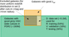 |
Fig. 1. Sketch of the available data and the intersection of the data D (dotted) used for training (R), validation (V), and testing (T) of the main network NetZmain, as presented in Sect. 4. |
As ground truth, we use the spectroscopic redshifts provided by the HSC team, which is a collection from various spectroscopic surveys (zCOSMOS DR3 (Lilly et al. 2009), UDSz (Bradshaw et al. 2013; McLure et al. 2012), 3D-HST (Skelton et al. 2014; Momcheva et al. 2016), VVDS (Le Fèvre et al. 2013), VIPERS PDR1 (Garilli et al. 2014), SDSS DR14 (Alam et al. 2015), GAMA DR2 (Liske et al. 2015), DEEP3 (Davis et al. 2003; Newman et al. 2013), PRIMUS DR1 (Coil et al. 2011; Cool et al. 2013)). Since we aim to obtain a network that is applicable to all morphological types, the above list does not include spectroscopic surveys that are most strongly biased towards specific galaxy types of similar morphology. Specifically, we do not consider objects from SDSS BOSS/eBOSS to train our main network NetZmain as those surveys explicitly target LRGs at z < 1 and known quasars. We do consider training exclusively on LRGs in our separate network NetZLRG. Furthermore, we do not include the WiggleZ catalog (Drinkwater et al. 2010), which targets UV bright emission line galaxies and which would further steepen the redshift distribution of the training set at low-redshift (see below). Despite unavoidable biases due to the selection function of each survey, we expect that this collection of spectroscopically-confirmed redshifts has limited morphological pre-selection. This spec-z sample is cleaned with the following criteria:
-
source type is GALAXY or LRG
-
z > 0
-
z ≠ 9.99992
-
0 < zerr < 1
-
the galaxy identification number (ID) is unique
-
specz_flag_homogeneous is False (homogenized spec-z flag from HSC team).
This spec-z sample is used in combination with COSMOS2015 (Laigle et al. 2018), a photo-z catalog of the COSMOS field based on around 30 available filters, where we enforce the following criteria:
-
flag_capak is False
-
type = 0 (only galaxies)
-
χ2(gal) < χ2(star) and χ2(gal)/Nbands < 5 (fits are reasonable and better than stellar alternatives)
-
ZP_2< 0 (no secondary peak)
-
log(M⋆) > 7.5 (stellar mass successfully recovered)
-
0 < z < 9
-
max(z84 − z50, z50 − z16) < 0.05(1 + z) (1σ-redshift dispersion < 5%).
This selection primarily follows the criteria from the other HSC photo-z methods (Tanaka et al. 2018; Nishizawa et al. 2020). We then select galaxies with i-band magnitudes brighter than 25 mag and a Kron radius larger than 0.8″ in the i band. The limit on the Kron radius is chosen with the aim of obtaining a set that best represents the sample that we are applying NetZ to. These criteria ensure that we have accurate and reliable reference redshifts for our training, validation, and testing. While such criteria could lead to potential selection bias in the objects, our combination of photo-z and spec-z helps mitigate selection biases. Furthermore, we verify that the color space spanned by the objects from the cleaned catalog is similar to that of the objects in the HSC PDR2 with a Kron radius above 0.8. This allows us to apply the trained NetZ based on the reference redshifts to those HSC PDR2 galaxies. The cleaned catalog used for training, validation, and testing is shown as a yellow box in Fig. 1, and the overlap with available good HSC images in all five filters (green box) contains 406 540 galaxies.
Based on various tests during the development stage, we found a significant improvement by masking the background and surrounding objects next to the galaxy of interest with the source extractor (Bertin & Arnouts 1996) before feeding them into the CNN. As a boundary, we use the 3σ level of the background. Fully deblended neighboring objects in the field can be excluded by requesting the object center to be within five pixels of the image center. With this method, we keep only the central galaxy(ies) in the image cutout. At the end we convolve the extracted image with a Gaussian kernel of size 3 × 3 pixels and a width of 1.5 pixels to smooth out the boundaries very slightly. We show color images of random galaxies from our NetZmain test sample in Fig. 2 as examples. The masked background is shown in blue and has pixel values set to zeros in the image. We provide the reference redshift, which can be either a spectroscopic or photometric redshift, and our predicted redshift at the top of each image. The HSC identification number is given in the bottom of each image. From these examples, it can be seen that the extraction procedure works well overall, but has its limitations; for instance, the first image of the second row is partly truncated because of a masked bright neighbouring object. Since this procedure is aimed at masking only obvious and well deblended companions, while beeing purposely conservative and retaining blended galaxies. Therefore, the third image in the first row in Fig. 2 is expected.
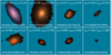 |
Fig. 2. Overview of galaxies from our data set. The masked neighbouring objects and background are shown in blue and have pixel values of zeros in the image. The images are 10.75″ × 10.75″ (64 × 64 pixels) and based on the three filters g, r, and i. In each panel, the reference and predicted redshifts of the object are indicated at the top and the HSC identification number is at the bottom. |
The reference redshift selection criteria described above give us a sample of galaxies with accurate reference redshifts, zref. Since the sample D is dominated by galaxies with zref < 1, we test the effect of data augmentation. Explicitly, we include rotated images for zref > 1, and in addition, mirrored images for zref > 2. An alternative to data augmentation is to introduce weights for the galaxies. For example, Lima et al. (2008) proposed a relative weighting of galaxies in order to match their spectroscopic sample to observables of the photometric sample. Although we could also adapt a similar weighting scheme to balance the redshift distribution, we favor the data augmentation technique that is commonly used in neural networks.
Since the distribution of the reference redshifts in the training set is very important for the network and still dominated by the lower redshift end, we limit each redshift bin of width 0.01 to have no more than 1000 galaxies from those passing the above criteria. With this limit, we obtain a uniform distribution up to zref ∼ 1.5. This essentially limits the number of low-redshift galaxies that would otherwise be over-represented in the training set. As a result, the redshift distribution becomes more uniform and allows the CNN to learn and predict redshifts for the full redshift range rather than only the lower redshift end. The excluded galaxy sample is marked in the underlying yellow box with lines in Fig. 1, while sample D is used for our main network NetZmain, shown with a red histogram in Fig. 3. We show the distribution of the augmented sample as a black dashed histogram in Fig. 3.
 |
Fig. 3. Histograms of the redshift samples used in this work. For NetZmain, we show the original redshift distribution in red, and the data augmented distribution in dashed black (with more galaxies at zref > 1) that was used for our final network. The distribution used to train our two specialized networks (see Sect. 6 for details) is overplotted for NetZlowz in blue and for NetZLRG in orange. |
3. Deep learning and the network architecture
Neural networks (NN) are very powerful tools that serve many different tasks, especially in works involving a huge amount of data. Substantial efforts have therefore been dedicated to deep learning (DL) developments in recent years. In general, for supervised learning, it is necessary to have a data set where the input and output, that is, the so-called ground truth, are known. On this data, the network is trained and can afterwards be applied to new data where the output is not known. The main advantages of NN include the variety of architectures and thus the broad range of problem they can be applied to, as well as the speed of those networks in comparison to other methods. Generally, there are two kinds of networks: classification networks distinguish between different classes of objects, whereas regression networks predict specific numerical quantities. The latter is the kind of network we are using here, namely it is the network that predicts a specific value for the redshift of a galaxy.
Depending on the task, there are different types of networks. Since our input consists of images of galaxies, a typical type is the CNN where the fully-connected (FC) layers are preceded by a number of convolutional (conv) layers. The detailed architecture depends on various parameters such the specific task, the size of the images, and the size of the data set. We tested different architectures and found an overall good network behavior with two convolutional layers followed by three FC layers. We tested different constructions of CNN architecture by varying the number of convolutional or FC layers, strides, and kernel sizes but with no improvement. A sketch of the final architecture is shown in Fig. 4. The input consists of five different filters for each galaxy and each image has a size of 64 × 64 pixels, corresponding to an image size of around 10″ × 10″. The convolutional layers have stride s = 1 and a kernel size of 5 × 5 × C, where C = 5 in the first convolutional layer, and C = 32 in the second layer. We used 32 kernels and 64 kernels in the first and second convolutional layers, respectively. Each convolutional layer is followed by max pooling of size 2 × 2 and of stride 2. This results in a data cube of size 13 × 13 × 64, which, after flattening, is passed on to the FC layers to obtain the single output value, namely, the redshift of the galaxy.
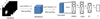 |
Fig. 4. Overview of the CNN architecture. It contains two convolutional (conv) layers with max pooling and three fully connected (FC) layers. The input consists of images of size 64 × 64 pixels in five different filters (grizy). The output displays the predicted photometric redshift. |
Independent of the network architecture, the network can contain hundreds of thousands (or more) neurons. Even though at the beginning, the values of the weight parameters and bias of each neuron are random, they are updated at every iteration of the training. To see the network performance after the training, we need to split the data into three sets, the training set R, the validation set V, and the test set T (see Fig. 1). In our case, we used 56% of the data set as training set, 14% as validation set, and 30% as test set. We trained over 300 epochs and divided each epoch into a number of iterations by splitting the training, validation, and test set into batches of a size N. In each iteration, a batch is passed through the entire network to predict the redshifts zpred (forward propagation). The difference between those predicted values and the ground truth is quantified by the loss function L, where we use the mean-square-error (MSE) defined as3
 (1)
(1)
After completing the forward propagation and computing the loss for the batch, the information is propagated to the weights and biases (back propagation) that are then modified using a stochastic gradient descent algorithm with a momentum of 0.9. This procedure is repeated for all batches in the training set and a total training loss for this epoch is thus obtained. Afterwards, the loss is computed within the validation set to determine the improvement of the network, which concludes the epoch.
We perform a so-called cross validation to minimize bias in the validation set, which comprises training the NN on the training set and using the validation set to validate the performance after each epoch as described above. These steps are repeated by exchanging the validation set within the training set, such that we have with our splitting five cross-validation runs. In the end, the network is trained on training and validation set together and terminated at the best epoch of all cross validation runs. The best epoch is defined as the epoch with the minimal average validation loss. This network is then applied to the test set, which contains data the network has never seen before.
4. Main redshift network NetZmain
In this section, we present our main network NetZmain which is trained in the full redshift range (0 < z ≲ 4). We find that this CNN is overall very precise in predicting redshifts. Figure 5 shows a comparison of our final network predictions zpred to the reference redshifts zref of the test set T. In detail, the left panel of this plot shows a histogram of the reference redshifts (red) and predicted values (blue). On the right panel, a 1:1 comparison of reference and predicted redshifts is plotted. The red line shows the median and the gray bands the 1σ and 2σ confidence levels.
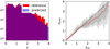 |
Fig. 5. Performance of the final network on the test set T. Left hand side: histograms of the reference and predicted redshift distributions in red and blue, respectively. Right hand side: a 1:1 comparison of reference and predicted redshifts. The red line shows the median predicted redshift per bin and the gray bands the 1σ and 2σ confidence levels. While the red line follows the black dashed reference line for low redshift very nicely, NetZmain tends to underpredict the high end. |
While the network performance is good in the redshift range between 0 and ∼2, the network starts to underestimate the higher redshifts. This is understandable as the network is trained on many more images in the lower reshift range as we can see directly from the histogram. The reason is the limited amount of available training data (reference redshifts) above z ∼ 2. Moreover, these distant galaxies are typically faint and small in extent, which complicates the learning procss with regard to their morphological features.
As described in Sect. 3, we use cross-validation and train always over 300 epochs. We do not see much overfitting from the loss curve, where overfitting means that after a certain number of epochs the network learns to predict the redshifts better for the training set than for the validation set. Based on our testing of different hyper-parameters such as batch size or learning rate, the best moment for terminating the training of NetZmain is at epoch 135 with a loss of 0.1107 according to the loss function L. This network has a learning rate of 0.0005 and a batch size of 128. We also tested drop-out, which means to ignore during each training epoch a new random set of neurons. This can help to reduce overfitting and balance the importance of the neurons in the network. We carried out a test using a dropout rate of 0.5 between the FC layers, but it turned out that drop-out was not necessary for this network.
We tested the network performance by varying the masking, such as the deblending threshold and the kernel for the smoothing. The difference of ≲0.01 in the predictions is small compared to the typical photo-z uncertainty (as we see in the scatter of Fig. 5). This network stability is important in case the extraction is not done perfectly as planned and done for the training. The masking is done in the exact same way for the newly predicted photo-z values as for training and testing.
It turns out that the network predicts similar but slightly different values for the augmented images, which shows that the network does not identify the rotated or mirrored images as duplicates. The possibility to use such data augmentation and hence boost the performance at high redshifts is a major strength of NetZ.
As a further test, we replaced the image cutouts of the galaxies with point-like sources using the corresponding PSF images and scaling them to the correct magnitudes. This way, the images contain only the information available from the catalogs (as used in typical photo-z methods) but exclude any morphological information such as the galaxy shapes from the real cutouts. We tested a few different hyper-parameter combinations by varying the learning rate and also the number of convolutional layers, but with the result of worse performance in predicting redshifts, as shown in Fig. 6. For more detail, we show on the left panel the performance of the network trained on the point-like images in analogy to the right panel of Fig. 5; and on the right panel, we make the direct comparison between the network trained on the correct image cutouts (red) and the network trained on images of point-like sources (blue). We can directly see the smaller scatter in the predicted redshift when using the correct cutouts, especially on the high-redshift range even with our use of data augmentation in this redshift range. This test shows the importance of the morphological information for this method and that it contributes significantly to the robustness of the photo-z predictions.
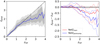 |
Fig. 6. Performance of the network trained on images of point-like sources in place of galaxies (blue) with 1 and 2 σ ranges on the left (gray), and as a comparison to NetZmain (red) on the right panel with 1σ ranges (dotted). We directly see that the original galaxy images and thus their morphological information improve the network. |
5. Comparison of NetZmain to other photo-z methods
5.1. Detailed comparison to HSC method DEmP
Since there are already different photo-z methods developed and applied to the HSC data, we show a comparison here. It is very important to use the same data set for a fair comparison. Thus, we can only make a comparison with the DEmP (Hsieh & Yee 2014) method, where we have a predicted photo-z value for each galaxy within our test set T and using identical training and validation sets as for NetZmain, without data augmentation – since DEmP also relies on the reference distribution. DEmP is one of the best-performing methods from the HSC photo-z team (Tanaka et al. 2018; Nishizawa et al. 2020) and, thus, it stands as a good performance benchmark. DEmP is a hybrid photo-z method by combining polynomial fitting and a N-nearest neighbor method based on photometric values on a catalog level. Therefore, the input data are totally different from those of NetZ, which is based on the pixelated image cutouts of the galaxies.
For the comparison, we adopted three quantities from the HSC photo-z papers (Tanaka et al. 2018; Nishizawa et al. 2020), which are defined as follows for each redshift bin:
 (2)
(2)
 (3)
(3)
 (4)
(4)
where i denotes the ith galaxy in the redshift bin, zpred the predicted photometric redshift, zref the reference redshift, N the number of galaxies satisfying the specified condition, and Nbin the total number of galaxies in the bin. The dispersion is defined using the median absolute deviation (MAD), as expressed above. The multiplication factor comes from statistics and is the relation factor for normally distributed data between MAD and the standard deviation (Rousseeuw & Croux 1993).
The comparison is shown in Fig. 7, with black triangles showing the performance of NetZmain and red bars showing the performance of DEmP. Since we use data augmentation (rotation and mirroring of images; see Sect. 2 for details) to increase the number of high-z galaxies, which is not possible for DEmP, we also trained a network without data augmentation – we show both in Fig. 7 for comparison. For the range zref ≲ 1.5, the performances of both methods are very good especially for the bias, with DEmP performing slightly better than NetZ. If we compare the range zref ≳ 1.5, the performance of both methods decreases, but NetZ with data augmentation now performs noticeably better than DEmP.
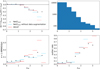 |
Fig. 7. NetZmain (black points) performance in terms of bias (top-left panel), dispersion (bottom-left panel), and outlier rate (bottom-right panel) as functions of the reference redshift zref in comparison to DEmP (red bars). Definitions of bias, dispersion and outlier rate are given in Eqs. (2)–(4). We show also with blue bars the results from a network where we do not use data augmentation to increase the number of high-z galaxies. The values in dashed bars are based on limited number of galaxies. The histogram in the top-right panel shows the number of galaxies as a function of redshift in the test set T used for the comparison. NetZ performs substantially better than DEmP at zref ≳ 2, with smaller bias, lower dispersion and lower outlier rate, by up to a factor of 2. |
A decrease in performance in the redshift range around z ≈ 2 is expected, as the used filter set grizy does not cover the prominent 4000 Å break but, in contrast to the other methods presented in Tanaka et al. (2018), NetZ and partly DEmP can at least break the degeneracy between low redshifts (z < 0.5) and the redshift range around 3–4, which is not the case for Mizuki from Nishizawa et al. (2020) and several methods from Tanaka et al. (2018) that used HSC images with similar reference redshifts. A more detailed and direct comparison is difficult since the predicted redshifts from these methods are not publicly available for our whole test set; moreover, some of the galaxies in our test set could be in the training data of these methods, which would artificially improve their performance.
The very low dispersion of DEmP in the highest-redshift bin comes from DEmP underestimating consistently most of the redshifts, and hence the outlier rate is large. Although the outlier rate is high in the range zref ≳ 2 in general, the performance is primarily limited by the number of existing reference redshifts in this range. While DEmP is developed and tested with a big enough training sample also for higher redshifts, we used here for DEmP the exact same data set as for NetZ for a fair comparison. Since there is no sufficient training sample at zref > 2 for both NetZ without data augmentation and DEmP, we plot these values in dashed because they are less reliable. It is nonetheless encouraging to see the significant reduction in the bias, dispersion, and outlier rate of NetZ with data augmentation for the high-z range, up to a factor of 2 relative to DEmP, thanks to the use of the spatial information from the galaxy images in addition to photometry. Especially for upcoming surveys such as LSST, which will provide relatively deep images, it is important to have methods prepared and tested on the higher redshift range.
As a further comparison, we show in Fig. 8 a scatter plot of zpred versus zref for DEmP (Hsieh & Yee 2014) and our neural network NetZmain with data augmentation. From this plot we can again see the good performance for the low-z range, where we note that the number of outliers from NetZ is negligible compared to the number of galaxies in the bins, which is also evident in the outlier rate. If we assume that all catastrophic outliers for zref < 1.5 are misplaced at high redshift, which is very conservative, then > 77% of the galaxies predicted to be at zpred > 1.5 are actually at zref > 1.5. In the high-z range, NetZ tends to predict too low redshifts, but it does not have the cluster of catastrophic outliers at zpred ∼ 0.5 and zref between 3 and 3.5 that DEmP does and this is due to the Lyman-break or Balmer-break misclassification. Even for the galaxies where the NetZ redshifts are classified as outliers, these redshifts are closer to the true redshift than for DEmP. The outlier rate for NetZ is dominated by blue-star-forming galaxies and galaxies with a small spatial extent (covering ≈20−30 pixels) that provide little information for the CNN to extract features. We therefore note that galaxies covering a small number of pixels are more prone to be catastrophic outliers in their redshifts and should be treated with caution.
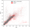 |
Fig. 8. Network performance as scatter plot comparing the predicted with the reference redshifts for NetZmain (this work) and DEmP (Hsieh & Yee 2014). The scatter looks overall comparable at zref ≲ 2, while NetZmain does not contain the catastrophic outliers at zref ∼ 3 and zpred ∼ 0.5 that DEmP has. |
5.2. Photo-z with morphological information
The studies presented by, for instance, Soo et al. (2018) and Wilson et al. (2020) aim to include morphological information of galaxies to improve photo-z estimations. In particular, Wilson et al. (2020) make use of optical and near infrared observations, some of which are obtained with the Hubble Space Telescope (HST). Therefore the considered data cover a wider wavelength range and are additionally of better spatial resolution than our ground based HSC images. However, Wilson et al. (2020) consider only photometric measurements and four morphological measurements (half-light radius, concentration, asymmetry, and smoothness), rather than the pixels directly. By working directly with the image pixels in our CNN, we use the maximal amount of information and we are independent of the pipelines and uncertainties when extracting morphological measurements. Moreover, Wilson et al. (2020) limit the range to 0 < z < 2, which makes the network not directly applicable to deep imaging surveys, especially since we are focusing on the high-redshift range. As we show in the next section, we also obtain very good results within a limited range. With these differences in the assumptions and data sets, it is difficult to directly compare the results of Wilson et al. (2020) and NetZ. Nonetheless, if we compare our outlier fraction with ∼0.05 up to z ∼ 1.7 (see Fig. 7) to that from Wilson et al. (2020), which is called OLF, with ∼0.1–0.2 up to z = 2 (see Tables 2 and 3 of Wilson et al. 2020), NetZ yields a good improvement. While Soo et al. (2018) and Wilson et al. (2020) find that morphological measurements do not provide a notable improvement in photo-z predictions when compared to using only multi-band photometric measurements, our NetZ results (Fig. 6) show that the pixels in the image cutouts that contain morphological information are useful. This suggests that a promising avenue for future developments of photo-z methods is to combine photometric measurements (as typically used for current photo-z methods) with direct image cutouts (as used for NetZ) instead of morphological measurements.
5.3. Photo-z estimates for LSST
Schmidt et al. (2020) present a collection of different photo-z methods tested on LSST mock data. In particular, they compare 12 different codes, of which three methods are based on template fitting (BPZ, Benítez 2000; EAZY, Brammer et al. 2008; LePhare, Arnouts et al. 1999), seven are based on machine learning (ANNz2, Sadeh et al. 2016; CMN, Graham et al. 2018; FlexZBoost, Izbicki et al. 2016; GPz, Almosallam et al. 2016a; METAPhoR, Cavuoti et al. 2017; SkyNet, Graff et al. 2014; TPZ, Carrasco Kind & Brunner 2013), one is a hybrid method (Delight, Leistedt & Hogg 2017), and one is a pathological photo-z PDF estimator method (trainZ, Schmidt et al. 2020). The last method trainZ is designed to serve as an experimental control, and not a competitive photo-z PDF method. It assigns to each galaxy set a photo-z PDF by effectively performing a k-nearest neighbor procedure. As training data, they use < 107 LSST like mock data limited to 0 < z < 2 and an i band magnitude limit of 25.3 to match the LSST gold sample (for further details see Schmidt et al. 2020). The main advantage of these methods in Schmidt et al. (2020) compared to the current version of NetZ is the probability density function estimates, whereas NetZ does not require photo-z pre-selection and shows a good performance over a broader redshift range (0 < z < 4). Based on the different redshift range and data sets, a detailed and fair comparison is not possible. If we compare Fig. 5 to Fig. B1 of Schmidt et al. (2020) quantitatively, we see an overall similar performance, but most of the LSST methods have a cluster of outliers at zref ∼ 0.5 and zref ∼ 1.7 which we do not see with NetZ. The kink at zref ∼ 1.7 might be related to the drop of data points and an edge effect near the end of the assumed range since we observe a similar effect with NetZ for higher redshifts (zref ∼ 3). Comparing the machine learning methods is difficult as well. The network architectures, as with nearest-neighbour algorithms, random forests, prediction trees, or sparse Gaussian processes, which are presented in Schmidt et al. (2020), are simply too different from the image-based CNN we present with NetZ.
6. Limited-range and LRG-only redshift network
During our testing, we found we could obtain substantial improvement by restricting the redshift range. We explored, for instance, networks with redshift ranges limited to 0 < z < 1 and 1 < z < 2, but not to higher redshift intervals, due to the limitations in available reference redshifts for z > 2. Limiting to 0 < z < 1 is also done in several other works (e.g., Hoyle 2016; Pasquet et al. 2019; Campagne 2020). To benefit from these refined networks in any practical application, we would first need to predict the correct redshift range and then these networks could be used in a specified range. We also considered combining multiple networks and iteratively refining the photo-z predictions, that is, start with NetZmain to predict zpred and then, based on the value of zpred, we could subsequently apply a network that is trained in a narrower range around zpred to refine the zpred estimate. However, we find that outliers from NetZmain limit the gain we can achieve in refining zpred. A practical possibility to use a redshift network for the lower-redshift end of the distribution would be to restrict the sample by the galaxy brightness. If we restrict our data set D to galaxies with an apparent i-band AB magnitude brighter than 22, the catalog includes only 1.3% objects with zref ≥ 1 and we miss 12.9% of all galaxies from the original set D with zref ≤ 1. For the training of NetZlowz itself we limit only to a narrow redshift range but not in magnitude. The performance of NetZlowz is shown in Fig. 9, on the left a histogram of the reference (red) and predicted (blue) redshifts. The distribution of the predicted redshift follows that of the reference redshift very well. On the right side, we show a 1:1 correlation plot, with the median as a red line and in gray the 1σ and 2σ areas. If we compare the two (Fig. 5), we can see that NetZlowz performs significantly better than NetZmain, as expected.
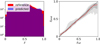 |
Fig. 9. Performance of the network NetZlowz trained on all types of galaxies in the range 0 < zref ≤ 1. Left hand side: histograms of the redshift distributions, in red the distribution of the reference redshifts used to train the network (ground truth) and in blue the predicted redshift distribution. Right panel: a 1:1 comparison of reference and predicted redshifts. The red lines show the median and the gray bands show the 1σ and 2σ confidence levels. |
We further show in Fig. 10 the bias, dispersion, and outlier rate for NetZlowz (red). If we compare this performance to NetZmain applied to the same galaxies for a fair comparison (blue), we find a good improvement in the bias and, with a factor of ∼2 reduction, in the dispersion. Only the outlier rate is comparable. If we compare the performance of NetZmain on the full test set that of the network, we still see an improvement for the network NetZlowz without the i magnitude limitation. This confirms that the improvement is related to the network range. A scatter plot of NetZlowz is shown in Fig. 11.
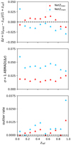 |
Fig. 10. Network performance of NetZlowz compared to NetZmain in terms of bias, dispersion, and outlier rate (see Eqs. (2)–(4)) as functions of the reference redshift zref. For this comparison, we use the overlap between both test sets and only galaxies with an i-band magnitude brighter than 22 as NetZlowz would be applied only to them. |
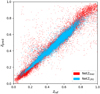 |
Fig. 11. Predicted redshifts zpred against the reference redshifts zref for the networks NetZLRG and NetZlowz of their test set. We see directly a lower outlier rate for NetZLRG than NetZlowz. |
Instead of applying networks trained for specific redshift ranges, which is difficult to do in practice, we can consider specific classes of galaxies that can be selected a priori, such as LRGs. Therefore we investigate a redshift estimation network specialized on LRGs that are useful for various studies including strong lensing and baryon acoustic oscillations. Since nearly all LRGs out of our reference sample have zpred < 1, we show here the network performance of NetZLRG in comparison to the network NetZlowz trained on all galaxy types. Figure 12 shows on the left a histogram and on the right the 1:1 comparison of zref and zpred.
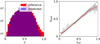 |
Fig. 12. Performance of the network NetZLRG (bottom) trained on LRGs only. Left-hand side: histograms of the redshift distributions in red we show the distribution of the reference redshifts used to train the network (ground truth) and in blue the predicted redshift distribution. Right panel: a 1:1 comparison of reference and predicted redshifts. The red lines show the median and the gray bands the 1σ and 2σ confidence levels. |
We show further the bias, dispersion, and outlier rate (defined in Eqs. (2)–(4)) in Fig. 13. The network NetZLRG performs better in most redshift bins. Finally, in Fig. 11 we show a scatter plot of this network without magnitude limitation in comparison to NetZlowz. From this we can see again the redshift limits of the LRG sample and also the good improvement.
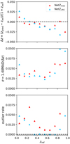 |
Fig. 13. Network performance of NetZLRG compared to NetZlowz applied to LRGs only in terms of bias, outlier rate, and dispersion (see Eqs. (2)–(4)) as functions of the reference redshift, zref. |
Both networks NetZLRG and NetZlowz show that photo-z for subsamples of galaxies does overall better than the main network NetZmain that is trained on all galaxies. Therefore, for specific subsamples, it would be beneficial to train a CNN specific to that sample.
7. Summary and conclusions
With current and upcoming imaging surveys, we anticipate that billions of galaxies will be the subject of observations, while just a small fraction of them will have spectroscopically confirmed redshifts. Therefore, it is necessary to have tools to obtain good photometric redshifts, especially for the higher redshift range as the upcoming surveys will provide deeper images where previous photo-z methods have strong limitations. With the success of ML and especially CNNs in image processing, we investigated a new CNN based technique to estimate the photo-z of a galaxy. The method is very general; it accepts directly cutouts of the observed images and predicts the corresponding redshift. Therefore it is directly applicable to all HSC cutouts after applying simple cuts on the Kron radius and i band magnitude observables.
For training the network and testing the performance, we carry out a comparison with to reference redshifts from various, mostly magnitude-limited surveys. In this paper, we focus on HSC data with a pixel size of 0.168″ and use the available five filters grizy, which are also part of the upcoming LSST4. In principle, it is also possible to include additional filters, such as the near-infrared (NIR) range from the same or a different telescope which would improve the performance even more, as shown by Gomes et al. (2018), for the low redshift range (z ≲ 0.6). The only constraint from the CNN is the constant pixel size over all different filters. Since NIR images have typically larger pixel sizes, an interpolation and resampling to the same pixel resolution as the optical images would be necessary. What remains to be seen is how much NetZ could benefit from such additional filters, especially in the high-z range, and this would need to be tested. In addition, NetZ could be trained on additional Euclid images that are high-resolution from space in the visible and infrared range. Even without combining Euclid with ground-based images, our photo-z estimates from HSC are useful for Euclid given the overlap in the footprints of HSC and Euclid.
With our trained network on HSC images, we find an overall very good performance of the network with a 1σ uncertainty of 0.12 averaged over all galaxies from the whole redshift range. Our CNN provides a point estimate for each galaxy with uncertainties adopted from the scatter in each redshift bin of the test set. Based on the amount of available data, the network performs better in the redshift range below z = 2. In the range above z = 2, we are using, as a way of gaining an advantage over state-of-the art methods like DEmP, data augmentation by rotating and mirroring the images. While the bias for DEmP and NetZmain as well as the dispersion for DEmP increases significantly in this range, with NetZmain we obtain by using data augmentation similar values as for the lower redshift range. We also obtain better outlier rates for the highest redshift bins by using data augmentation but the improvement is less pronounced. In particular, NetZ does not under-predict the redshifts of galaxies with zref ∼ 3−3.5 by as much as DEmP and other methods due to the Lyman and Balmer break misclassification. The main limitations that all photo-z methods face when predicting redshifts for distant galaxies is the low number of reference redshifts. In our case, the number drops by a factor of around 1000 compared to the range where z < 2. Therefore, using the image cutouts gives a good advantage as we can use data augmentation by rotating and mirroring the images. The effect is impressive as one can see in Fig 7. Since this is not possible for other photo-z methods, several of them focus only on the lower redshift range z < 1 or even lower (e.g., Hoyle 2016; Pasquet et al. 2019; Campagne 2020). If we also limit the redshift range to z < 1, we find a substantial improvement in our network‘s performance.
In cases where we set our focus on a specific galaxy type like LRGs, we find a further improvement with regard to the network. This is understandable as the network can learn better the specific features of this galaxy type. Based on the small number of LRGs with redshift above z = 1, we limit the range of NetZLRG to 0 < z < 1 and compare it to a network trained on all galaxy types in the same redshift range for a fair comparison.
This paper provides a proof of concept for using a CNN for photo-z estimates. Based on the encouraging results of NetZ particularly at high redshifts, we propose further investigations along the lines of combining our CNN with a nearest-neighbor algorithm or a fully-connected network that ingests catalog-based photometric quantities (see Leal-Taixé et al. 2016). There are several methods, like DEmP and other methods (e.g. D’Isanto & Polsterer 2018; Schmidt et al. 2020), which provide a probability distribution function for the redshifts. Further developments of our CNN approach to provide a probability distribution function of the photo-z require more complex networks such as Bayesian neural networks (e.g., Perreault Levasseur et al. 2017) or mixture density networks (D’Isanto & Polsterer 2018; Hatfield et al. 2020; Eriksen et al. 2020). While this is beyond the scope of the current paper, such Bayesian or mixture networks are worth exploring.
In this work, we show that a very simple convolutional neural network is able to predict accurate redshifts directly from the observed galaxy images. NetZ therefore has the advantage of using maximal information from the intensity pixels in the galaxy images, rather than relying on photometric or morphological measurements that could be prone to uncertainties and biases, especially for images of blended galaxies. We ran NetZmain on 34 414 686 galaxies from the HSC public data release 2 (PDR2) wide survey and provide the catalog here5. We flagged all negative predictions and clear catastrophic outliers (zpred > 5), which are 15 043 and 3314 objects, respectively, as −99. In Fig. 14, we show a histogram of the newly available photo-z values (blue filled), whose distribution resembles the magnitude-limited sample of the cleaned COSMOS2015 (Laigle et al. 2018, orange histogram), which was scaled by a factor of 1010, to have the same sample size for the purposes of making a direct comparison. This check shows that our NetZ predictions indeed produce a realistic galaxy redshift distribution expected for a depth similar to that of LSST.
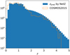 |
Fig. 14. Histogram of the newly predicted photo-z values with NetZ based on images of the HSC PDR2 (blue filled) and, for comparison, the distribution of COSMOS2015 (Laigle et al. 2018) scaled by a factor of 1010 to have the same sample size (orange open). The similarity in the two distributions shows that NetZ produces a realistic galaxy redshift distribution. |
As the image quality, depth and processing of HSC and LSST first-year data are expected to be similar (the image processing pipeline of HSC is a branch of the LSST pipeline), the method we have developed here will be directly applicable and beneficial to the LSST. The additional u-filter in the LSST will likely further improve photo-z predictions. When applying our method to the LSST data, we do not expect to necessarily have to test the network architecture, however, it is likely that some hyper-parameter combinations would need testing. Since training is more optimally carried out on real images, rather than on mock images as done, for instance, in Schmidt et al. (2020, and references therein), we suggest that it is optimal to train a new network on LSST images as soon as they are available.
HSC webpage: https://hsc-release.mtk.nao.ac.jp/doc/
This is the upper limit of the catalog and thus treated as no spec-z available, i.e. excluded.
This definition is for only one parameter, which in our case is the redshift. For a general expression, one would also sum over the different parameters.
LSST has in addition u-band observations.
The catalog is available at https://www.dropbox.com/sh/grjfo0gkcxsj9n2/AAD-B7D6m7_1i6GGTX0Ionwja?dl=0
Acknowledgments
We thank Andreas Breitfeld from our IT group for helpful support. S. S., S. H. S., and R. C. thank the Max Planck Society for support through the Max Planck Research Group for SHS. This project has received funding from the European Research Council (ERC) under the European Union’s Horizon 2020 research and innovation programme (LENSNOVA: grant agreement No 771776). The Hyper Suprime-Cam (HSC) collaboration includes the astronomical communities of Japan and Taiwan, and Princeton University. The HSC instrumentation and software were developed by the National Astronomical Observatory of Japan (NAOJ), the Kavli Institute for the Physics and Mathematics of the Universe (Kavli IPMU), the University of Tokyo, the High Energy Accelerator Research Organization (KEK), the Academia Sinica Institute for Astronomy and Astrophysics in Taiwan (ASIAA), and Princeton University. Funding was contributed by the FIRST program from Japanese Cabinet Office, the Ministry of Education, Culture, Sports, Science and Technology (MEXT), the Japan Society for the Promotion of Science (JSPS), Japan Science and Technology Agency (JST), the Toray Science Foundation, NAOJ, Kavli IPMU, KEK, ASIAA, and Princeton University. This paper is based in part on data collected at the Subaru Telescope and retrieved from the HSC data archive system, which is operated by Subaru Telescope and Astronomy Data Center (ADC) at National Astronomical Observatory of Japan. Data analysis was in part carried out with the cooperation of Center for Computational Astrophysics (CfCA), National Astronomical Observatory of Japan. We make partly use of the data collected at the Subaru Telescope and retrieved from the HSC data archive system, which is operated by Subaru Telescope and Astronomy Data Center at National Astronomical Observatory of Japan.
References
- Aihara, H., Arimoto, N., Armstrong, R., et al. 2018, PASJ, 70, S4 [NASA ADS] [Google Scholar]
- Aihara, H., AlSayyad, Y., Ando, M., et al. 2019, PASJ, 71, 114 [CrossRef] [Google Scholar]
- Alam, S., Albareti, F. D., Prieto, C. A., et al. 2015, ApJS, 219, 12 [NASA ADS] [CrossRef] [Google Scholar]
- Almosallam, I. A., Lindsay, S. N., Jarvis, M. J., & Roberts, S. J. 2016a, MNRAS, 455, 2387 [NASA ADS] [CrossRef] [Google Scholar]
- Almosallam, I. A., Jarvis, M. J., & Roberts, S. J. 2016b, MNRAS, 462, 726 [NASA ADS] [CrossRef] [Google Scholar]
- Arnouts, S., Cristiani, S., Moscardini, L., et al. 1999, MNRAS, 310, 540 [NASA ADS] [CrossRef] [Google Scholar]
- Benítez, N. 2000, ApJ, 536, 571 [Google Scholar]
- Bertin, E., & Arnouts, S. 1996, A&AS, 117, 393 [NASA ADS] [CrossRef] [EDP Sciences] [Google Scholar]
- Bolzonella, M., Miralles, J. M., & Pelló, R. 2000, A&A, 363, 476 [NASA ADS] [Google Scholar]
- Bonnett, C. 2015, MNRAS, 449, 1043 [NASA ADS] [CrossRef] [Google Scholar]
- Bonnett, C., Troxel, M. A., Hartley, W., et al. 2016, Phys. Rev. D, 94, 042005 [NASA ADS] [CrossRef] [Google Scholar]
- Bradshaw, E. J., Almaini, O., Hartley, W. G., et al. 2013, MNRAS, 433, 194208 [NASA ADS] [CrossRef] [Google Scholar]
- Brammer, G. B., van Dokkum, P. G., & Coppi, P. 2008, ApJ, 686, 1503 [NASA ADS] [CrossRef] [Google Scholar]
- Campagne, J. E. 2020, ArXiv e-prints [arXiv:2002.10154] [Google Scholar]
- Carliles, S., Budavári, T., Heinis, S., Priebe, C., & Szalay, A. S. 2010, ApJ, 712, 511 [NASA ADS] [CrossRef] [Google Scholar]
- Carrasco Kind, M., & Brunner, R. J. 2013, MNRAS, 432, 1483 [NASA ADS] [CrossRef] [Google Scholar]
- Cavuoti, S., Amaro, V., Brescia, M., et al. 2017, MNRAS, 465, 1959 [NASA ADS] [CrossRef] [Google Scholar]
- Coil, A. L., Blanton, M. R., Burles, S. M., et al. 2011, ApJ, 741, 8 [Google Scholar]
- Collister, A. A., & Lahav, O. 2004, PASP, 116, 345 [NASA ADS] [CrossRef] [Google Scholar]
- Cool, R. J., Moustakas, J., Blanton, M. R., et al. 2013, ApJ, 767, 118 [NASA ADS] [CrossRef] [Google Scholar]
- Coupon, J., Ilbert, O., Kilbinger, M., et al. 2009, A&A, 500, 981 [NASA ADS] [CrossRef] [EDP Sciences] [Google Scholar]
- Dahlen, T., Mobasher, B., Faber, S. M., et al. 2013, ApJ, 775, 93 [Google Scholar]
- Davis, M., Faber, S. M., Newman, J., et al. 2003, Discoveries and Research Prospects from 6- to 10-Meter-Class Telescopes II [Google Scholar]
- D’Isanto, A., & Polsterer, K. L. 2018, A&A, 609, A111 [NASA ADS] [CrossRef] [EDP Sciences] [Google Scholar]
- Drinkwater, M. J., Jurek, R. J., Blake, C., et al. 2010, MNRAS, 401, 14291452 [NASA ADS] [CrossRef] [Google Scholar]
- Duncan, K. J., Jarvis, M. J., Brown, M. J. I., & Röttgering, H. J. A. 2018, MNRAS, 477, 5177 [Google Scholar]
- Eriksen, M., Alarcon, A., Cabayol, L., et al. 2020, MNRAS, 497, 4565 [CrossRef] [Google Scholar]
- Feldmann, R., Carollo, C. M., Porciani, C., et al. 2006, MNRAS, 372, 565 [NASA ADS] [CrossRef] [Google Scholar]
- Garilli, B., Guzzo, L., Scodeggio, M., et al. 2014, A&A, 562, A23 [NASA ADS] [CrossRef] [EDP Sciences] [Google Scholar]
- Gomes, Z., Jarvis, M. J., Almosallam, I. A., & Roberts, S. J. 2018, MNRAS, 475, 331 [NASA ADS] [CrossRef] [Google Scholar]
- Graff, P., Feroz, F., Hobson, M. P., & Lasenby, A. 2014, MNRAS, 441, 1741 [NASA ADS] [CrossRef] [Google Scholar]
- Graham, M. L., Connolly, A. J., Ivezić, Ž., et al. 2018, AJ, 155, 1 [NASA ADS] [CrossRef] [Google Scholar]
- Hatfield, P. W., Almosallam, I. A., Jarvis, M. J., et al. 2020, MNRAS, 498, 5498 [CrossRef] [Google Scholar]
- Hildebrandt, H., Wolf, C., & Benítez, N. 2008, A&A, 480, 703 [NASA ADS] [CrossRef] [EDP Sciences] [Google Scholar]
- Hildebrandt, H., Arnouts, S., Capak, P., et al. 2010, A&A, 523, A31 [NASA ADS] [CrossRef] [EDP Sciences] [Google Scholar]
- Hildebrandt, H., Erben, T., Kuijken, K., et al. 2012, MNRAS, 421, 2355 [Google Scholar]
- Hoyle, B. 2016, Astron. Comput., 16, 34 [NASA ADS] [CrossRef] [Google Scholar]
- Hsieh, B. C., & Yee, H. K. C. 2014, ApJ, 792, 102 [NASA ADS] [CrossRef] [Google Scholar]
- Izbicki, R., Lee, A. B., & Freeman, P. E. 2016, ArXiv e-prints [arXiv:1604.01339] [Google Scholar]
- Laigle, C., Pichon, C., Arnouts, S., et al. 2018, MNRAS, 474, 5437 [NASA ADS] [CrossRef] [Google Scholar]
- Leal-Taixé, L., Canton Ferrer, C., & Schindler, K. 2016, ArXiv e-prints [arXiv:1604.07866] [Google Scholar]
- Le Fèvre, O., Cassata, P., Cucciati, O., et al. 2013, A&A, 559, A14 [NASA ADS] [CrossRef] [EDP Sciences] [Google Scholar]
- Leistedt, B., & Hogg, D. W. 2017, ApJ, 838, 5 [NASA ADS] [CrossRef] [Google Scholar]
- Lilly, S. J., Le Brun, V., Maier, C., et al. 2009, ApJS, 184, 218 [Google Scholar]
- Lima, M., Cunha, C. E., Oyaizu, H., et al. 2008, MNRAS, 390, 118 [Google Scholar]
- Liske, J., Baldry, I. K., Driver, S. P., et al. 2015, MNRAS, 452, 2087 [NASA ADS] [CrossRef] [Google Scholar]
- McLure, R. J., Pearce, H. J., Dunlop, J. S., et al. 2012, MNRAS, 428, 1088 [NASA ADS] [CrossRef] [Google Scholar]
- Momcheva, I. G., Brammer, G. B., van Dokkum, P. G., et al. 2016, ApJS, 225, 27 [NASA ADS] [CrossRef] [Google Scholar]
- Newman, J. A., Cooper, M. C., Davis, M., et al. 2013, ApJS, 208, 5 [Google Scholar]
- Nishizawa, A. J., Hsieh, B. C., Tanaka, M., & Takata, T. 2020, ArXiv e-prints [arXiv:2003.01511] [Google Scholar]
- Pasquet-Itam, J., & Pasquet, J. 2018, A&A, 611, A97 [NASA ADS] [CrossRef] [EDP Sciences] [Google Scholar]
- Pasquet, J., Bertin, E., Treyer, M., Arnouts, S., & Fouchez, D. 2019, A&A, 621, A26 [NASA ADS] [CrossRef] [EDP Sciences] [Google Scholar]
- Perreault Levasseur, L., Hezaveh, Y. D., & Wechsler, R. H. 2017, ApJ, 850, L7 [NASA ADS] [CrossRef] [Google Scholar]
- Rousseeuw, P. J., & Croux, C. 1993, J. Am. Stat. Assoc., 88, 1273 [CrossRef] [Google Scholar]
- Sadeh, I., Abdalla, F. B., & Lahav, O. 2016, PASP, 128, 104502 [NASA ADS] [CrossRef] [Google Scholar]
- Schmidt, S. J., Malz, A. I., Soo, J. Y. H., et al. 2020, MNRAS, 499, 1587 [Google Scholar]
- Singal, J., Shmakova, M., Gerke, B., Griffith, R. L., & Lotz, J. 2011, PASP, 123, 615 [NASA ADS] [CrossRef] [Google Scholar]
- Skelton, R. E., Whitaker, K. E., Momcheva, I. G., et al. 2014, ApJS, 214, 24 [Google Scholar]
- Soo, J. Y. H., Moraes, B., Joachimi, B., et al. 2018, MNRAS, 475, 3613 [NASA ADS] [CrossRef] [Google Scholar]
- Tagliaferri, R., Longo, G., Andreon, S., et al. 2003, Neural Networks for Photometric Redshifts Evaluation, 2859, 226 [Google Scholar]
- Tanaka, M., Coupon, J., Hsieh, B.-C., et al. 2018, PASJ, 70, S9 [Google Scholar]
- Wilson, D., Nayyeri, H., Cooray, A., & Häußler, B. 2020, ApJ, 888, 83 [CrossRef] [Google Scholar]
- Wolf, C. 2009, MNRAS, 397, 520 [NASA ADS] [CrossRef] [Google Scholar]
All Figures
|
Fig. 1. Sketch of the available data and the intersection of the data D (dotted) used for training (R), validation (V), and testing (T) of the main network NetZmain, as presented in Sect. 4. |
| In the text | |
|
Fig. 2. Overview of galaxies from our data set. The masked neighbouring objects and background are shown in blue and have pixel values of zeros in the image. The images are 10.75″ × 10.75″ (64 × 64 pixels) and based on the three filters g, r, and i. In each panel, the reference and predicted redshifts of the object are indicated at the top and the HSC identification number is at the bottom. |
| In the text | |
|
Fig. 3. Histograms of the redshift samples used in this work. For NetZmain, we show the original redshift distribution in red, and the data augmented distribution in dashed black (with more galaxies at zref > 1) that was used for our final network. The distribution used to train our two specialized networks (see Sect. 6 for details) is overplotted for NetZlowz in blue and for NetZLRG in orange. |
| In the text | |
|
Fig. 4. Overview of the CNN architecture. It contains two convolutional (conv) layers with max pooling and three fully connected (FC) layers. The input consists of images of size 64 × 64 pixels in five different filters (grizy). The output displays the predicted photometric redshift. |
| In the text | |
|
Fig. 5. Performance of the final network on the test set T. Left hand side: histograms of the reference and predicted redshift distributions in red and blue, respectively. Right hand side: a 1:1 comparison of reference and predicted redshifts. The red line shows the median predicted redshift per bin and the gray bands the 1σ and 2σ confidence levels. While the red line follows the black dashed reference line for low redshift very nicely, NetZmain tends to underpredict the high end. |
| In the text | |
|
Fig. 6. Performance of the network trained on images of point-like sources in place of galaxies (blue) with 1 and 2 σ ranges on the left (gray), and as a comparison to NetZmain (red) on the right panel with 1σ ranges (dotted). We directly see that the original galaxy images and thus their morphological information improve the network. |
| In the text | |
|
Fig. 7. NetZmain (black points) performance in terms of bias (top-left panel), dispersion (bottom-left panel), and outlier rate (bottom-right panel) as functions of the reference redshift zref in comparison to DEmP (red bars). Definitions of bias, dispersion and outlier rate are given in Eqs. (2)–(4). We show also with blue bars the results from a network where we do not use data augmentation to increase the number of high-z galaxies. The values in dashed bars are based on limited number of galaxies. The histogram in the top-right panel shows the number of galaxies as a function of redshift in the test set T used for the comparison. NetZ performs substantially better than DEmP at zref ≳ 2, with smaller bias, lower dispersion and lower outlier rate, by up to a factor of 2. |
| In the text | |
|
Fig. 8. Network performance as scatter plot comparing the predicted with the reference redshifts for NetZmain (this work) and DEmP (Hsieh & Yee 2014). The scatter looks overall comparable at zref ≲ 2, while NetZmain does not contain the catastrophic outliers at zref ∼ 3 and zpred ∼ 0.5 that DEmP has. |
| In the text | |
|
Fig. 9. Performance of the network NetZlowz trained on all types of galaxies in the range 0 < zref ≤ 1. Left hand side: histograms of the redshift distributions, in red the distribution of the reference redshifts used to train the network (ground truth) and in blue the predicted redshift distribution. Right panel: a 1:1 comparison of reference and predicted redshifts. The red lines show the median and the gray bands show the 1σ and 2σ confidence levels. |
| In the text | |
|
Fig. 10. Network performance of NetZlowz compared to NetZmain in terms of bias, dispersion, and outlier rate (see Eqs. (2)–(4)) as functions of the reference redshift zref. For this comparison, we use the overlap between both test sets and only galaxies with an i-band magnitude brighter than 22 as NetZlowz would be applied only to them. |
| In the text | |
|
Fig. 11. Predicted redshifts zpred against the reference redshifts zref for the networks NetZLRG and NetZlowz of their test set. We see directly a lower outlier rate for NetZLRG than NetZlowz. |
| In the text | |
|
Fig. 12. Performance of the network NetZLRG (bottom) trained on LRGs only. Left-hand side: histograms of the redshift distributions in red we show the distribution of the reference redshifts used to train the network (ground truth) and in blue the predicted redshift distribution. Right panel: a 1:1 comparison of reference and predicted redshifts. The red lines show the median and the gray bands the 1σ and 2σ confidence levels. |
| In the text | |
|
Fig. 13. Network performance of NetZLRG compared to NetZlowz applied to LRGs only in terms of bias, outlier rate, and dispersion (see Eqs. (2)–(4)) as functions of the reference redshift, zref. |
| In the text | |
|
Fig. 14. Histogram of the newly predicted photo-z values with NetZ based on images of the HSC PDR2 (blue filled) and, for comparison, the distribution of COSMOS2015 (Laigle et al. 2018) scaled by a factor of 1010 to have the same sample size (orange open). The similarity in the two distributions shows that NetZ produces a realistic galaxy redshift distribution. |
| In the text | |
Current usage metrics show cumulative count of Article Views (full-text article views including HTML views, PDF and ePub downloads, according to the available data) and Abstracts Views on Vision4Press platform.
Data correspond to usage on the plateform after 2015. The current usage metrics is available 48-96 hours after online publication and is updated daily on week days.
Initial download of the metrics may take a while.