| Issue |
A&A
Volume 666, October 2022
|
|
|---|---|---|
| Article Number | A85 | |
| Number of page(s) | 12 | |
| Section | Extragalactic astronomy | |
| DOI | https://doi.org/10.1051/0004-6361/202244081 | |
| Published online | 11 October 2022 | |
Galaxy morphoto-Z with neural Networks (GaZNets)
I. Optimized accuracy and outlier fraction from imaging and photometry
1
School of Astronomy and Space Science, University of Chinese Academy of Sciences, Beijing 100049, PR China
e-mail: This email address is being protected from spambots. You need JavaScript enabled to view it.
2
National Astronomical Observatories, Chinese Academy of Sciences, 20A Datun Road, Chaoyang District, Beijing 100012, PR China
3
School of Physics and Astronomy, Sun Yat-sen University, Zhuhai Campus, 2 Daxue Road, Xiangzhou District, Zhuhai, PR China
e-mail: This email address is being protected from spambots. You need JavaScript enabled to view it.
4
CSST Science Center for Guangdong-Hong Kong-Macau Great Bay Area, Zhuhai, 519082, PR China
5
Yunnan Observatories, Chinese Academy of Sciences, Kunming, 650011 Yunnan, PR China
6
INAF – Osservatorio Astronomico di Capodimonte, Salita Moiariello 16, 80131 Napoli, Italy
7
Center for Theoretical Physics, Polish Academy of Sciences, Al. Lotników 32/46, 02-668 Warsaw, Poland
8
INFN – Sezione di Napoli, via Cinthia 9, 80126 Napoli, Italy
9
INAF – Osservatorio Astronomico di Padova, via dell’Osservatorio 5, 35122 Padova, Italy
Received:
22
May
2022
Accepted:
16
July
2022
Abstract
Aims. In the era of large sky surveys, photometric redshifts (photo-z) represent crucial information for galaxy evolution and cosmology studies. In this work, we propose a new machine learning (ML) tool called Galaxy morphoto-Z with neural Networks (GaZNet-1), which uses both images and multi-band photometry measurements to predict galaxy redshifts, with accuracy, precision and outlier fraction superior to standard methods based on photometry only.
Methods. As a first application of this tool, we estimate photo-z for a sample of galaxies in the Kilo-Degree Survey (KiDS). GaZNet-1 is trained and tested on ∼140 000 galaxies collected from KiDS Data Release 4 (DR4), for which spectroscopic redshifts are available from different surveys. This sample is dominated by bright (MAG_AUTO < 21) and low-redshift (z < 0.8) systems; however, we could use ∼6500 galaxies in the range 0.8 < z < 3 to effectively extend the training to higher redshift. The inputs are the r-band galaxy images plus the nine-band magnitudes and colors from the combined catalogs of optical photometry from KiDS and near-infrared photometry from the VISTA Kilo-degree Infrared survey.
Results. By combining the images and catalogs, GaZNet-1 can achieve extremely high precision in normalized median absolute deviation (NMAD = 0.014 for lower redshift and NMAD = 0.041 for higher redshift galaxies) and a low fraction of outliers (0.4% for lower and 1.27% for higher redshift galaxies). Compared to ML codes using only photometry as input, GaZNet-1 also shows a ∼10%−35% improvement in precision at different redshifts and a ∼45% reduction in the fraction of outliers. We finally discuss the finding that, by correctly separating galaxies from stars and active galactic nuclei, the overall photo-z outlier fraction of galaxies can be cut down to 0.3%.
Key words: surveys / galaxies: general / techniques: photometric / galaxies: photometry
© R. Li et al. 2022
 Open Access article, published by EDP Sciences, under the terms of the Creative Commons Attribution License (https://creativecommons.org/licenses/by/4.0), which permits unrestricted use, distribution, and reproduction in any medium, provided the original work is properly cited.
This article is published in open access under the Subscribe-to-Open model. This email address is being protected from spambots. You need JavaScript enabled to view it. to support open access publication.
1. Introduction
In the last decade, the Stage III sky surveys, such as the Kilo-Degree Survey (KiDS, de Jong et al. 2013), Hyper Suprime-Cam (HSC; Aihara et al. 2018), and the Dark Energy Survey (DES; The Dark Energy Survey Collaboration 2005), have provided images of hundreds of millions of galaxies at optical or near-infrared (NIR) wavelengths. These surveys have achieved significant advances in cosmology (e.g., Hildebrandt et al. 2017; Hikage et al. 2019; Abbott et al. 2022) and galaxy formation and evolution (e.g., Roy et al. 2018; Greco et al. 2018; Goulding et al. 2018; Adhikari et al. 2021), but at the same time have left many open questions about the overall cosmological model (Di Valentino et al. 2021).
In the next decade, the Stage IV surveys (Weinberg et al. 2013), such as Euclid (Laureijs et al. 2011), Vera Rubin Legacy Survey in Space and Time (VR/LSST; Ivezić et al. 2019), and China Space Station Telescope (CSST; Zhan 2018), will observe billions of galaxies with photometric bands ranging from the ultraviolet (UV) to the NIR. This unprecedented amount of data will help us to obtain deeper insight into cosmology and galaxy evolution. For instance, we will be able to gain a more detailed understanding of the dark matter distribution in the Universe, constrain the equation of state of the dark energy with weak lensing (e.g., Laureijs et al. 2011; Hildebrandt et al. 2017; Abbott et al. 2018; Gong et al. 2019; Joachimi et al. 2021; Heymans et al. 2021), study the mass–size relation of galaxies at higher redshift (z > 1.0), and explore the stellar and dark matter assembly in galaxies and clusters (e.g., Yang et al. 2012; Moster et al. 2013; Behroozi et al. 2019, Tortora & Napolitano 2022) over enormous statistical samples.
To achieve real breakthroughs in these areas, accurate galaxy redshifts are essential, as, by providing object distances and lookback time, they allow those objects to be traced back in time. Precise redshifts can only be estimated from galaxy spectra: current spectroscopic surveys, such as the Sloan Digital Sky Survey (SDSS, Ahumada et al. 2020), the Galaxy and Mass Assembly (GAMA Baldry et al. 2018a), and the Dark Energy Spectroscopic Instrument (DESI, DESI Collaboration 2016) have collected data for millions of galaxies, while future surveys, such as the 4-meter Multi-Object Spectroscopic Telescope (4MOST, de Jong et al. 2019), plan to expand spectroscopic measurements to samples of hundreds of millions of galaxies. However, due to the limited observation depth and prohibitive exposure times, it is impossible to spectroscopically follow up the even larger and fainter samples of billions of galaxies expected in future imaging surveys.
A fast, low-cost alternative is offered by photometric redshifts (photo-z) estimated from deep, multi-band photometry. The idea of photo-z was initially proposed by Baum (1962), who used a redshift–magnitude relation to predict the redshifts from the galaxy luminosities. Without spectroscopic observations and the knowledge of galaxy evolution, the relation could still provide acceptable redshifts, even using only a limited number of filters. Later, this method was adopted to extensively estimate galaxy redshifts (e.g., Couch et al. 1983; Koo 1985; Connolly et al. 1995; Connolly 1997; Wang et al. 1998). Nevertheless, albeit straightforward, this method has some limitations: (1) the redshift–magnitude relation is inferred in advance from bright galaxies via spectroscopy, and (2) the relation is hard to extend to fainter galaxies. Another method used to determine photo-z is spectral-energy-distribution(SED) fitting. This method is based on galaxy templates, both theoretical and empirical.
By fitting the observed multi-band photometry to the SED from galaxy templates, one can infer individual galaxy photo-z. With knowledge of galaxy types and their evolution with redshift, this method can be expanded to faint galaxies, and even extrapolated to redshifts higher than the spectroscopic limit. There is a variety of photo-z codes based on SED fitting. Among the most popular ones is HyperZ (Bolzonella et al. 2000), which makes use of multi-band magnitudes of galaxies and the corresponding errors to best fit the SED templates by minimizing a given χ2 function. An extension of HyperZ, known as Bayesian photometric redshifts (BPZ, Benítez 2000), is another popular photo-z tool. Instead of simple χ2 minimization, BPZ introduces prior knowledge of the redshift distribution of magnitude-limited samples under a Bayesian framework, which effectively reduces the number of catastrophic outliers in the predictions.
In addition to these fitting tools, machine learning (ML) algorithms, especially artificial neural networks (ANNs), have started to be extensively used to determine galaxy photo-z (e.g., Collister et al. 2007; Abdalla et al. 2008; Banerji et al. 2008). Given a training sample of galaxies with spectroscopic redshifts, ML algorithms can learn the relationship between redshift and multi-band photometry. If the training sample covers a representative redshift range and the ML model is well trained, photo-z can be obtained with extremely high precision. Different tools for photo-z based on ML have been successfully tested on multi-band photometry data, for example estimating photo-z with ANNs (ANNz, Collister & Lahav 2004; ANNz2 Sadeh et al. 2016) or the Multi-Layer Perceptron trained with the Quasi-Newton Algorithm (MLPQNA, Cavuoti et al. 2012, Amaro et al. 2021).
Accurate photometry measurements are extremely important for ML and SED fitting methods, as the presence of noisy or biased photometry would end up in large scatter and a high outlier fraction in the predicted values. For instance, biased photometry is typically produced in the case of close galaxy pairs or in the presence of bright neighbors. In addition, there are well-known degeneracies between color and redshift plaguing late-type systems, in particular, as high-z star-forming galaxies can be confused with lower redshift ellipticals. These examples suggest that there might be some crucial information encoded in images that can help in solving the typical systematic errors that affect the methods based on photometry only.
Machine learning has been shown to be able to learn galaxy properties such as size, morphology, and their environment from images. This information can help suppress catastrophic errors and improve the accuracy of the photo-z predictions. In recent years, many studies have been trying to estimate photo-z directly from multi-band images using deep learning. A first attempt was presented by Hoyle (2016), where they estimated photo-z with a deep neural network (DNN) applied to full galaxy imaging data. More recently, a similar approach was applied to data from the Sloan Digital Sky Survey and Hyper Suprime-Cam Subaru Strategic Program (e.g., D’Isanto & Polsterer 2018; Pasquet et al. 2019; Schuldt et al. 2021; Dey et al. 2021). These analyses showed that unbiased photo-z can be estimated directly from multi-band images. A more simplistic method for taking morphology features into account, such as size, ellipticity, and Sérsic index, was proposed by Soo et al. (2018), who added structural parameters to the photometric catalogs used in standard ANNs.
In this paper, we develop a new ML method to estimate the morphoto-z, that is, redshifts estimated from the combination of images and catalogs of photometry and color measurements. In the following, we distinguish these morphoto-z from the redshift predicted from photometry only, the classical photo-z, and from the redshift obtained from images only, which, for convenience, we call morpho-z. This is the first time such a technique has been developed and applied to real data: specifically, we use optical images and optical+NIR multi-band photometry from the KiDS survey. Just before the submission of this paper, a similar approach was proposed by Zhou et al. (2022), but this latter work is based on (CSST) simulated data only.
This work is organized as follows. In Sect. 2, we describe how to build the ML models and to collect the training and testing samples. In Sect. 3, we train the networks and show the performance of the tools. In Sects. 4 and 5, we discuss the results and draw some conclusions.
2. The ML method
In this work, we intend to couple standard ML regression tools –usually applied to galaxy multi-band photometry– with Deep Learning techniques in order to improve the estimates of galaxy redshifts using the information from features distilled from galaxy images. In particular, we want to address the following questions: (1) We would like to know whether or not redshifts can be estimated directly from multi-band images of KiDS galaxies, and how the typical accuracy compares to that achieved with ML tools based on integrated photometry and color measurements only. (2) We would also like to know how much improvement in precision and scatter images and catalogs can add to tools when combined.
To answer these questions, we have developed and compared four ML tools to estimate the galaxy redshifts. These differ from one another in terms of the type of input data they can work with. In this section, we start by describing the structures and the training of these four tools.
2.1. Network architectures
The ML parts of our networks are constituted by ANNs. These have been shown to work well on catalogs made of magnitudes and color measurements (e.g., Collister et al. 2007; Abdalla et al. 2008; Banerji et al. 2008; Cavuoti et al. 2015; Brescia et al. 2014; de Jong et al. 2017; Bilicki et al. 2018, 2021). A typical ANN structure consists of three main parts: input, hidden, and output layers. The input and the output layers are used to load the data in the network and to issue the predictions. The hidden layers, composed of fully connected artificial neurons in a sequence of multiple layers, are used to extract features. These features are subsequently abstracted to allow the networks to determine the final outputs. In redshift estimates, the inputs of the networks are catalogs of some form of multi-band aperture photometry of galaxies, that is, measurements of the total flux in different filters, usually from the optical to NIR wavelengths.
The deep learning components of the four tools are convolutional neural networks (CNN, Cun et al. 1990), which are an effective family of algorithms for feature extraction from images. CNNs mimic the biological perception mechanisms with convolution operations. This makes them especially suitable for image processing, pattern recognition, and other tasks relative to images (e.g., Domínguez Sánchez et al. 2018; Ackermann et al. 2018; Walmsley et al. 2020; Ćiprijanović et al. 2020; Li et al. 2020, 2022, 2021; Tohill et al. 2021). CNNs have become popular years after their introduction because of the significant progress in graphics processing unit (GPU) technology.
Below, we introduce the structures of the first series of algorithms for “Galaxy morphoto-Z with neural Networks” (GaZNets). These are introduced to derive galaxy morpho-z and photo-z using different combinations of inputs, including multi-band photometry and imaging (see Fig. 1).
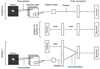 |
Fig. 1. Machine learning models used in this work. Top: CNN structure of GaZNet-I4 with only galaxy images as input. Middle: ANN structure of GaZNet-C4 and GaZNet-C9, with only catalog as input. Bottom: structure of GaZNet-1, fed by both galaxy images and the corresponding catalogs. |
– GaZNet-I4. This is a CNN model that makes use of galaxy images in four optical bands (u, g, r, i), with a cutout size of 8 × 8″ (corresponding to 40 × 40 pixels; see Sect. 2.2) as input. The model is a slightly modified architecture from VGGNet (Simonyan & Zisserman 2014). It is constituted of four blocks made of different numbers of convolutional layers. Each of the first two blocks contains two layers, and the other two blocks each contain three layers. After the four blocks, a flatten layer is used to transform the high-dimensional features into one-dimensional features. Finally, we adopt three fully connected layers to combine the low-level features into higher level ones and output the predicted redshift.
– GaZNet-C4. This is a simple ANN structure with two blocks each made of four fully connected layers separated by a flatten layer. The input is an optical four-band (u, g, r, i) catalog of magnitude and color measurements. As we use the information from the same bands, comparing GaZNet−I4 and GaZNet−C4 allows us to quantify the impact of the imaging and photometry on the redshift estimates.
– GaZNet-C9. This has the same structure as GaZNet−C4, but is input with the four-band optical catalogs from KiDS plus the five-band catalogs from the VISTA Kilo-degree Infrared Galaxy survey (VIKING, Edge & Sutherland 2014, see Sect. 2.2 for details). Using a broader wavelength baseline, GaZNet−C9 will allow us to estimate the impact of the multi-band coverage on the ANN redshift predictions.
– GaZNet-1. This is the reference network we have developed: the input is a combination of the r-band images and the multi-band photometry catalogs. GaZNet-1 has been designed to have a two-path structure. The first path comprises four blocks, as in GaZNet−I4, while the second is made of eight fully connected layers, as in GaZNet−C4 and C9. After a flatten layer, the features from each path are concatenated together. Finally, five fully connected layers are added to combine the features from images and catalogs to generate the final redshift predictions.
Of the four tools illustrated above, the first three are mainly designed to test the impact of the different inputs on the final redshift estimates. Being constructed with the same structure assembled in the final GaZNet-1, that is, the one to be used for science, they guarantee the homogeneity of the treatment of the input data (see Fig. 1).
In this first series of GaZNets, we do not consider the magnitude ratios between different bands as inputs, although there are experiments suggesting that they can improve the precision (see e.g., D’Isanto et al. 2018, Nakoneczny et al. 2019). We plan to implement this in future analyses, because here we are interested in checking the advantages of the combination of images and photometry compared to previous analyses made on the same data (see Sect. 3.2.3). Also, in this analysis, we focus on redshift point estimates. In the future, we plan to expand the capabilities of the GaZNets to estimate the probability density function p(z) for each galaxy. This can be achieved by mixture density networks (e.g., Rhea et al. 2021, Wang et al. 2022) or Bayesian networks (Gal & Ghahramani 2015; Kendall & Gal 2017), and some studies have been carried out with these two networks (e.g., D’Isanto & Polsterer 2018; Ramachandra et al. 2022; Podsztavek et al. 2022). We also evaluate the performance of the p(z) using a cumulative distribution function (CDF) and CDF-based metrics, such as the Kolmogorov-Smirnov (KS) statistic, the Cramer-von Mises statistic, and the Anderson-Darling (AD) statistic (see details in Schmidt et al. 2020).
2.2. Training and testing data
The dataset used in this work is collected from KiDS and VIKING, two twin surveys covering the same 1350 deg2 sky area, in optical and NIR bands, respectively. KiDS observations are carried out with the VST/Omegacam telescope (Capaccioli & Schipani 2011; Kuijken 2011) in four optical filters (u, g, r, i), with a spatial resolution of 0.2″/pixel. The r-band images are observed with the best seeing (average FWHM ∼ 0.7″), and its mean limiting AB magnitude (5σ in a 2″ aperture) is 25.02 ± 0.13. The seeing of the other three bands (u, g and i) is slightly poorer than that of the r-band, namely FWHMs < 1.1″, and the mean limiting AB magnitudes are also fainter, namely 24.23 ± 0.12, 25.12 ± 0.14, 23.68 ± 0.27 for u, g, and i, respectively (Kuijken et al. 2019).
VIKING is carried out with the VISTA/VIRCAM (Sutherland et al. 2015) and was designed to complement KiDS observations with five NIR bands (Z, Y, J, H and Ks). The median value of the seeing in the images is ∼0.9″ (Sutherland et al. 2015), and the AB magnitude depths are 23.1, 22.3, 22.1, 21.5, and 21.2 in the five bands (Edge et al. 2013), respectively.
In particular, the galaxy sample used in this work is made of 148 521 objects for which spectroscopic redshifts (spec-zs, hereafter) are available from different surveys, such as the Galaxy And Mass Assembly survey (GAMA, Driver et al. 2011) data release 2 and 3, the zCOSMOS (Lilly et al. 2007), the Chandra Deep Field South (CDFS, Szokoly et al. 2004), and the DEEP2 Galaxy Redshift Survey (Newman et al. 2013). The spec-z range of the galaxies covers quite a large baseline, in the range ∼0 − 7, although the distribution is far from uniform. Indeed, as shown in Fig. 2, the number of galaxies at higher redshift (z ≳ 0.8) is much smaller than the one at lower redshift. In the same figure, we can see a peak of distribution at spec-z < 0.6. It comes from the GAMA survey, which is the most complete spectroscopic survey adopted, with ∼95.5% completeness for r-band magnitude MAG_AUTO < 19.8 (Baldry et al. 2018a). Similarly, we see a second peak at spec-z ∼ 2.5, which is due to the quite deep observations from zCOSMOS. Overall, this sample is dominated by bright and low-redshift galaxies (0.04 < z < 0.8), but in the range 0.8 < z < 3 it still contains about 6500 galaxies with a relatively uniform redshift distribution that can be used as a training sample to extend the predictions to higher redshift. Due to the unbalanced redshift coverage, we expect the accuracy of the predictions to show significant variation with redshift. However, we check if the final estimates meet the accuracy and precision requirements for cosmological and galaxy formation studies (see e.g., LSST Science Collaboration 2009). After this redshift cut, the final sample is made of 134 148 galaxies. The distributions of the r-band Kron-like magnitude, MAG_AUTO, obtained by SExtractor (Bertin & Arnouts 1996) for these galaxies, and their signal-to-noise ratio (S/N; defined as the inverse value of the error of MAG_AUTO) are also reported in Fig. 2. Finally, the 134 148 galaxies are divided into three datasets, 100 000 for training, 14 148 for validation, and 20 000 for testing and error statistical analysis.
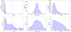 |
Fig. 2. Distribution of some relevant parameters of the training and testing data. In the top row, number counts are in linear scale, while in the bottom row number counts are in logarithmic scale. The first panel on the left shows the original spectroscopic sample of the 148 521 galaxies collected in KiDS+VIKING. However, only the 134 148 galaxies located between the two vertical dashed lines (spec-z = 0.04 and spec-z = 3) are used in this work for training and testing the GaZNets. For these galaxies, we show the MAG_AUTO and S/Ns in the second and third panels. |
The u, g, r, i band images, with a size of 8 × 8″, are cutout from KiDS DR4 (Kuijken et al. 2019). The corresponding catalogs, made up of nine Gaussian Aperture and Point spread function (GAaP) magnitudes (u, g, r, i, Z, Y, J, H, Ks) and eight derived colors (e.g., u − g, g − r, r − i, etc.), are directly selected from the KiDS public catalog1. The GAaP magnitudes have been measured on Gaussian-weighted apertures, modified per source and per image, thereby providing seeing-independent flux estimates across different observations and bands, and reducing the bias of colors (see detail in Kuijken et al. 2015, 2019). The extinction was also considered in the measurement of the GAaP magnitudes.
2.3. External photo-z catalog by MLPQNA
To test the performances of GaZNet-1 against other ML-based photo-z methods, we collected an external photo-z catalog obtained from MLPQNA for the same KiDS galaxies that we used as a testing sample. This allows us to perform a quantitative comparison of diagnostics such as accuracy, scatter, and fractions of outliers.
MLPQNA is an effective computing implementation of neural networks adopted for the first time to solve regression problems in an astrophysical context. A test on the PHAT1 dataset (Hildebrandt et al. 2010) indicated that MLPQNA, with smaller bias and fewer outliers, performs better than most of the traditional standard SED-fitting methods. This code has been used in some current sky surveys; for example in KiDS (Cavuoti et al. 2015) and the Sloan Digital Sky Survey (SDSS; Brescia et al. 2014). For our comparison, we adopt the MLPQNA photo-z catalog from Amaro et al. (2021), where these authors used the same data presented in Sect. 2.2 to train and test their networks.
3. GaZNet training and testing
In Sect. 2.1 we describe the different GaZNets and anticipate that they accept either images or catalogs of galaxies as inputs, except the GaZNet-1, which is given both images and catalogs as input. In particular, for the first test of morphoto-z predictions made with this latter, we choose only the r-band images, that is, the ones with best quality from KiDS, to combine with the nine-band photometry catalog. As we demonstrate in Sect. 4, the multi-band imaging does not add a detectable improvement in the results in exchange for the higher computation time required. In this section, we illustrate the procedures to train the networks and test their predicted photo-zs against the ground truth provided by the spec-zs of the test sample introduced in Sect. 2.2.
3.1. Training the networks
We train the networks by minimizing the “Huber” loss (see, Huber 1964; Friedman 1999) function with an “Adam” optimizer (Kingma & Ba 2014). The Huber loss is defined as
 (1)
(1)
in which a = ytrue − ypred. ytrue is the spec-z and ypred is the predicted photo-z. Here, δ is a parameter that can be pre-set. Given a δ (fixed to 0.001 in this work), the loss will be a square error when the deviation of the prediction, |a|, is smaller than δ; otherwise, the loss is reduced to a linear function. Compared to the commonly used mean square error (MSE) or mean absolute error (MAE) loss function, defined as
 (2)
(2)
Huber loss has proven to be more accurate in such regression tasks (see detailed discussion in Li et al. 2022).
To guarantee that the loss function loses speed more quickly, for each ML model, we set a larger learning rate of 0.001 at the beginning and train the networks for 30 epochs. In each epoch, the networks are trained on the training data and validated on the validation data to decipher whether or not further adjustments are needed to improve the overall accuracy. After the first training round, we reduce the learning rate to 0.0001, and load the pre-trained model with a “callback” operation. We then train the networks for a further 30 epochs. Reducing the learning rate to 0.0001 can help the network to converge to the global minimum, where it finds the best-trained model.
For the networks input with images, we also apply some data augmentations, including random shift, flip, and rotation (only 90° ,180° and 270°). We do not adopt any augmentation that requires interpolation algorithms2, such as crop, zoom, color changing, or addition of noise, because these operations would change the flux in the image pixels, affecting the magnitudes and colors of the galaxies.
Regarding computation time, with the NVIDIA RTX 2070 graphics processing unit (GPU), GaZNet-C4 and GaZNet-C9 require 28 min to complete the training and validation process, while GaZnet-1 takes about 134 min (including ∼2.5 min for data reading) because of the time needed to process the r-band image data along with the magnitudes and colors. Compared with GaZNet-1, GaZNet-I4 does not significantly increase the time required for the training and validation process. However, to deal with the four-channel images, it needs more GPU memory, and the duration of data reading increases significantly. Finally, GaZNet-I4 requires about four times as much data reading time as compared to GaZNet-1. We also estimated that to make predictions on 20 000 galaxies (see Sect. 3.2), GaZNet-C9 needs only ∼6 s for the whole galaxies, while GaZNet-1 needs ∼55 s, including ∼30 s for data reading and ∼25 s for prediction.
3.2. Testing the performance
After the training phase, we use the 20 000 testing galaxies to estimate the precision and the statistical errors of the redshift predictions from different GaZNets.
3.2.1. Statistical parameters
We define a series of statistical parameters to describe the overall performances: (1) the fraction of catastrophic outliers, (2) the mean bias, and (3) the normalized median absolute deviation (NMAD).
The fraction of the catastrophic outliers is defined as the fraction of galaxies with bias larger than 15% according to the following formula:
 (3)
(3)
where zspec are the spec-zs of the test galaxies and zpred are the predicted redshifts by the ML tools. This definition is usually adopted for outliers in photo-z estimates (see details in e.g., Cavuoti et al. 2012, Amaro et al. 2021) and gives a measure of the fallibility of the method. In addition, the mean bias in this work is labeled as μδz.
The NMAD between the predicted photo-zs and the true spec-zs, is defined as
 (4)
(4)
where δz comes from Eq. (3). The NMAD allows us to quantify the scatter of the overall predictions in comparison to the ground truth, and therefore is a measurement of the precision of the redshift estimates from the ML tools.
3.2.2. Predictions versus ground truth
The testing results on 20 000 galaxies for the four GaZNets are shown in Fig. 3, where on the x-axis we plot the spec-zs as ground truth, and on the y-axis we plot the predicted redshifts. As a comparison, in the same figure, we also show the photo-zs estimated by the MLPQNA. We divided the galaxies into six redshift bins, and computed the mean absolute errors, shown as error bars, and the mean |δz| defined in Eq. (3), reported as text. We use equally spaced bins to check the effect of the sampling as a function of the redshift.
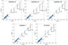 |
Fig. 3. Comparison between the spectroscopic redshifts and the predicted photometric redshifts for different models. From top left to bottom right are the results from GaZNet-I, GaZNet-C, GaZNet, and MLPQNA, respectively. Error bars represent the mean absolute errors (MAEs), while the quoted numbers are the mean |δz| in each bin. |
From Fig. 3, a major feature noticeable at the first glance is the odd coverage of the spec-z at high redshift (z ≳ 0.8), which we also discuss in Sect. 2.2. This is a potential issue for all methods, as a poor training set can introduce a large scatter in the predictions. Indeed, in Fig. 3, the δz tends to have an increasingly large scatter toward larger redshifts. This means that at z ≳ 0.8 the absolute scatters are dominated by the size of the training sample rather than the true intrinsic uncertainties of the methods. Unfortunately, this is a problem we cannot overcome with the current data and we need to wait for larger spec-z data samples in order to improve the precision at higher redshifts. However, given the current training set, we can still evaluate the relative performances of different methods and their ability to make accurate predictions even in the small training set regimes.
To go into detail, from Fig. 3 we see that unbiased photo-z can be obtained by GaZNet-I4, with only four-band images as input, although it seems that this starts to deviate from the one-to-one relation at z ≳ 1.5. However, at these redshifts, a general trend of underestimating the ground truth is also shown by GaZNet-C4 and GaZNet-C9, although the latter uses the full photometry from the KiDS+VIKING dataset. Interestingly, looking at the scatter, GaZNet-I4 seems to perform better than GaZNet-C4 at all redshift bins and almost comparably to C9 in most cases.
The results from GaZNet-I4 demonstrate that the morpho-z values from multi-band images are similar if not potentially superior to photo-zs values from photometry in the same bands. This high-performance of morpho-zs is also confirmed by the noticeably smaller outlier fraction (1.5% for GaZNet-I4 and 2.2% for GaZNet-C4 in general). Even more interestingly, looking from the perspective of future surveys relying on a narrower wavelength baseline, such as the space missions Euclid and CSST, our results show that morpho-zs are not far from optical+NIR large photometric baselines in terms of accuracy, scatter, and the fraction of outliers. This is particularly true for z < 1, where, as seen in Fig. 3, the GaZNet-I4 shows fewer outliers than GaZNet-C9, while this latter shows a rather lower fraction of outliers at higher redshifts.
Moving to GaZNet-C9, the results show the impact of the broader wavelength baseline including the five NIR bands. Generally, photo-z determined by GaZNet-C9 shows improved indicators in comparison to GaZNet-I4 and GaZNet-C4. From Fig. 3, we can see these coming from a better linear correlation, especially at z > 1.5, and smaller absolute errors. However, looking at the results in more detail, at z > 1.5 the presence of a rather large fraction of outliers causes the median values to diverge from the one-to-one relationship in a way similar to GaZNet-I4 and GaZNet-C4. It is hard to assess whether this is caused by the poor training sample, or is an intrinsic shortcoming of the ML tool. In either cases, it is important to check whether or not using the information from images can improve this result.
Compared to GaZNet-C9, GaZNet-1 shows better performance overall, with a tighter one-to-one relation, and smaller errors (by ∼10 − 35%) in all redshift bins. This is shown in the bottom-left panel of Fig. 3. This result leads us to two main conclusions: (1) images (even a single high-quality band; see Sect. 4 for the test on multi-band imaging) provide crucial information for solving intrinsic issues related to the photometry only and improve all performances of the redshift predictions in terms of accuracy, scatter, and outlier fraction; we discuss the reason for this in Sect. 4; (2) due to the poor redshift coverage of the training sample at z > 1, the results we have obtained possibly represent a lower limit on the potential performances of the tool. In any case, the GaZNet-1 reaches an excellent overall precision of δz = 0.038(1 + z) up to z = 3, with an overall outlier fraction of 0.74%.
3.2.3. Test versus external catalogs
We can finally compare the performance of the four GaZNets versus the external catalogs. The MLPQNA is rather similar to the ANN method used for the GaZNets-C9, as it makes use of a similar algorithm and the same catalogs from KiDS DR4. From Fig. 3, we see that MLPQNA performs similarly to GaZNet-I4 and better than GaZNet-C4. This is not surprising as the MLPQNA uses a larger wavelength baseline. This is particularly visible at higher redshift, where the predictions from MLPQNA are more tightly distributed around the one-to-one relationship with the ground truth than GaZNet-I4 and GaZNet-C4.
3.2.4. Performance in space of redshift and magnitude
In the preceding subsections, we demonstrate that GaZNet-1 shows better performance than other tools in terms of accuracy and precision. However, in Fig. 3, we also see a variation of this performance as a function of redshift. Here, we want to quantify this effect in more detail, as well as the dependence on the magnitudes of the same performances. The reason for this diagnostic is to assess the impact of selection effects on overall performance (see e.g., van den Busch et al. 2020). For example, in Sect. 3.2.2, we anticipate that the redshift sampling by the training sample can be one source of degradation of performance at z > 1.
In Fig. 4 we plot the outlier fraction (out. fr.), mean bias (μδz), and scatter (NMAD) as functions of spec-z, photo-z, and r-band magnitude. For comparison, we plot the same relations for GaZNet-C9 and MLPQNA, the other two tools showing comparable performances to GaZNet-1. The bottom row of Fig. 4 finally shows the distribution of the training sample in the same parameter space.
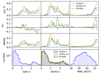 |
Fig. 4. Outlier fraction (out. fr.), mean bias (μδz), and scatter (NMAD) as functions of spec-z, photo-z, and magnitude in 20 bins. In each panel, the blue line is for GaZNet-1, orange is for GaZNet-C9, and green is for MLPQNA. In the last row, we also present the number distribution in the corresponding parameter space. |
This figure gives the overall impression that GaZNet-1 generally performs better than the other two tools in most if not all redshift and magnitude bins, with lower outlier fraction, mean bias, and scatter. We also see a clear correlation of the performances of all tools, including GaZNet-1, with the size and magnitude of the training sample in different redshift bins and at different magnitudes of the training galaxies All three tools perform relatively well in the range of z ≲ 0.8, where the training sample is about one order of magnitude larger, resulting in a more accurate training. To quantify the overall performance in this redshift range, in Table 1 we report the global statistical parameters for these galaxies. All three tools can achieve relatively small outlier fractions (≲0.01), mean bias (close to 0), and scatter (≲0.022). Of the three tools, GaZNet-1 shows the best performance. In particular, its outlier fraction is 43% smaller than GaZNet-C9 and 60% smaller than MLPQNA.
Statistical properties of the predictions.
In Fig. 4, we see that the number of galaxies decreases rapidly at z ≳ 0.8, which produces a degradation of the performance of all three tools. Interestingly, looking at the central panels, after z ∼ 1.5, where the COSMOS spec-z sample is concentrated, the performances, especially in terms of scatter (NMAD), show a significant improvement up to z ≳ 2.6, where the spec-z of the training sample quickly drops in number again. This is also quantified in Table 1 by the global statistical parameters for these higher redshift galaxies. Compared to GaZNet-C9, all the indicators from GaZNet-1 are significantly improved. The fraction of outliers, the mean bias, and the scatter are decreased by 46%, 58%, and 44%, respectively. On the other hand, MLPQNA remains the tool that shows the poorest performance. A similar behavior in performance is seen as a function of photo-z, as this latter closely follows spec-z (see Fig. 3).
Regarding magnitude space, we find that all indicators show very small values at MAG_AUTO ≲ 21, which means that the redshift estimates for brighter galaxies are highly reliable. After r-band MAG_AUTO ∼ 21, all indicators degrade, showing a worsening of the accuracy, precision, and outlier fraction. However, in this respect, among the three tools, GaZNet-1 shows the best performance. In particular, after MAG_AUTO ∼ 22, there is a peak at 30%, which could be driven by the poorer S/N of the systems, but is more likely caused by the smaller statistics. Nevertheless, in general, the GaZNet-1 still has a relatively small outlier fraction (∼1.0%).
Overall, it is clear that collecting more galaxies covering higher redshift (z ≳ 0.8) and fainter magnitudes (MAG_AUTO ≳ 22) will be essential for improving the performance of these ML tools, and the results collected here simply represent a lower limit on the real performance that these tools can achieve, especially GaZNet-1. However, even with the current training set, GaZNet-1 can provide results that satisfy the requirements for weak gravitational lensing studies in next generation ground-base surveys, even for high-redshift galaxies (e.g., NMAD = 0.05 in VR/LSST, LSST Science Collaboration 2009), although this has only been tested here on a relatively bright sample with AB magnitude MAG_AUTO ≤ 22 (see Sect. 4). For the low-redshift samples, GaZNet-1 is already well within the requirements for the same surveys and is virtually ‘science ready’. In the future, we will look for more higher redshift galaxies from different spectroscopic surveys to build a less biased training sample and improve the performances at z > 0.8.
4. Discussion
In the preceding section, we compare the performances of the different GaZNets based on different architectures, both with and without the inclusion of deep learning. We also compare the GaZNets against external catalogs of photo-z based on traditional ML algorithms. The reason for developing different tools with an increasing degree of complexity is to understand the impact of the different features on the final predictions. The main conclusion of this comparison is that GaZNet-1, which uses a combination of nine-band photometry and r-band imaging, clearly outperforms the other tools –either developed by us or taken from the literature–which take only photometry as input and do not use deep learning. We also see how deep learning only, applied to only four-band optical images, can produce morpho-z of greater accuracy than the photo-z from the corresponding photometry and can match the performance of the nine-band photometry, except at redshifts of z > 0.8. Overall, we find that part of the superior performance of deep learning is its ability to reduce the outlier fraction. In this section, we investigate the reasons for these findings and discuss the impact of some of the choices we made in the setup of the GaZNets presented in this first paper.
4.1. Outliers
From Table 1, it is evident that the major advantage of deep learning when applied to high-quality imaging resides in the low outlier fraction. For GaZNet-1, this is smaller than that of GaZNet-C9 by ∼43% for low-redshift galaxies (z < 0.8) and 46% for higher redshift galaxies (z > 0.8). Understanding the reasons for these results is important for identifying the source of the systematic errors and for planning future developments for more accurate morphoto-z estimates.
To investigate the genesis of these outliers, we start by checking the galaxies for which the ML tools fail to obtain accurate photo-zs. In Fig. 5, we show the optical gri color-composed and the r-band images of representative outliers from GaZNet-C9, which are no longer outliers for GaZNet-1. In each r-band image, we report the spec-z ot the top, the GaZNet-C9 photo-z in the bottom-left corner, and the GaZNet-1 morphoto-z in the bottom-right corner. For comparison, in Fig. 5, we also show outliers from GaZNet-C9 that are still outliers for GaZNet-1. The color images in this figure provide a relatively good idea of the galaxy SEDs, while the r-band images illustrate the corresponding “morphological” features that the GaZNet-1 uses to improve the overall predictions.
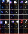 |
Fig. 5. g, r, i color-composited color images (20″ × 20″) and the corresponding r-band images for some representative outliers. Rows A, B, C, and D (blue framed) show the outliers in GaZNet–C9, which are no longer outliers in GaZNet-1 predictions. Rows E, F, and G (red framed) show the objects that remain outliers both for GaZNet-1 and GaZNet-C9. In the r-band images, we report spec-z at the top, the GaZNet-C9 photo-z in the bottom left, and the GaZNet-1 morphoto-z in the bottom right. |
From Fig. 5, we can distinguish four kinds of outliers for GaZNet-C9. The first one (A-row) is made of galaxies that are close to bright and often saturated stars or large bright galaxies. In some cases, GaZNet-1 can improve the predictions and solve the discrepancy with the ground-truth values (A-row). However, in some other cases, the environment is too confused to allow the CNN to guess correctly, despite the CNN being able to deblend the embedded source (E-row; see discussion below). The second type of outlier (B-row) is irregular galaxies or, generally, diffuse nearby systems. These systems are generally star forming and blue, similarly to the majority of high-redshift galaxies. Thus, they typically have a higher chance of being confused with higher-z systems. In this case, GaZNet-1 can recognize the complex morphology (knots, substructures, pseudo-arms, etc.), or a noisier surface-brightness distribution, which are typical features of closer galaxies3. The third type of outlier (C-row) is merging or interacting systems. For these systems, GaZNet-1 can solve the discrepancy using information about the size of the two systems and the degree of detail of the substructures, making the predictions of these systems relatively accurate. The fourth type of outlier (D-row) is blue objects, generally high-z compact systems, sometimes also at low-z. In this case, again, GaZNet-1 can make more accurate predictions from the size and the round morphology.
With this insight into the ways in which deep learning can help to improve the predictions of photo-z, we can now check where it still fails. This might give us valuable indications as to how we can improve GaZNet-1 performances in future analyses. In Fig. 5 we see three types of outliers also for GaZNet-1. The first (E-row), similarly to those for GaZNet-C9 in the A-row above, is caused by the presence of large, bright systems. In these cases, GaZNet-1 has difficulty in either correctly deblending the source or correctly evaluating the size, especially if very compact. However, we stress here that these outliers are generally fewer than all of the other kinds (∼5% of the total outliers for both GaZNet-1 and C9), and in the case of bright stars can often be automatically masked out from catalogs. The second type (F-row) is galaxies whose size appears to be at odds with their redshift; for example small-sized low-z objects (which could be ultra-compact galaxies or misclassified stars, etc.) or even large-sized high-z systems (which could be very massive or high-luminosity systems, or galaxies with large diffuse haloes, etc.). As for the previous type, these systems are also relatively limited in number (∼4%), and their failure also depends on the poor training sample. In general, these outliers do not represent a significant issue. The third type (G-row) is extremely compact, almost point-like and generally blue sources. These are the most abundant sample of outliers (∼58%). Although their redshift distribution is relatively sparse, they have a very similar appearance, being mainly concentrated at z > 1 but with cases even at z < 0.5. There is little chance that all these systems are misclassified as stars or very compact blue galaxies (e.g., blue nuggets), although we cannot exclude that some of them are indeed misclassified. The only possible option is that these are galaxies hosting active galactic nuclei (AGNs) or quasars. If so, these represent a marginal fraction of the training sample, and for this reason, they are not accurately predicted.
The SED of a quasar is different from that of a typical galaxy (e.g., Feng et al. 2021), and a small fraction of quasars may not provide enough training samples. In addition, most quasars can present strong variability, because they are observed in different bands at different times. This introduces fictitious color terms that increase the uncertainties on photo-z measurements. To verify this assumption, we check the star–galaxy–quasar separation in Khramtsov et al. (2019) based on an ML classifier. We find that only ∼35% of the 147 outliers are classified as galaxies. For the remaining ∼65%, about half are classified as quasars and half as stars. Regardless of the accuracy of the ML method to classify stars and quasars, this analysis confirms that only a minority of the catastrophic events are galaxies, which is consistent with our guess based on the visual inspection above. In particular, the three objects in Fig. 5-G are all quasars in the ML classification.
If indeed the outliers are dominated by misclassified stars and AGNs or quasars, we can reasonably assume that optimizing the classification of these groups of contaminants would reduce the overall outlier fraction down to a very small value, ∼0.3%.
4.2. Other tests
The four GaZNets illustrated in Sect. 2.1 and discussed in Sects. 3.2.2 and 4 are the results of a selection process from a number of other models that we have tested with different kinds of inputs and different ML structures. Among these models, we focus on two other experiments where we have tested two setups that, in principle, can impact the final results. The parameters describing the performances of these two further configurations are shown in Table 2. Below, we summarize their properties and the major results:
Statistical properties of the predictions.
1. GaZNet-81pix to test the cutout size. The GaZNets work on images with a size of 8″ × 8″, which might be too small to collect the light of the entire galaxies and their environments, thus leaving some important features that the CNNs cannot see. In order to check for this possibility, we tested the GaZNet-1 on images with twice the size of each side (16″ × 16″). Compared with the previous result in Table 2, the parameters remain almost unchanged. A possible reason is that the features that the CNNs extract from images are concentrated in the high-S/N regions of the galaxies, while the outer regions bring little information about either the galaxy properties or the environment that might otherwise be used to improve the redshift estimates. Using these arguments, one could ask whether or not the standard 8″ × 8″ cutouts could be replaced with smaller cutouts whilst obtaining the same performance. To check this possibility, we also tested 4″ × 4″ and found slightly poorer results, and so we kept the 8″ × 8″ as the best choice.
2. GaZNet-C9I4 to test the nine-band catalogs plus four-band images. GaZNet-1 makes use of nine-band catalogs and only r-band images. To check if the addition of images in other bands can produce a discernable improvement, we trained a GaZNet with the four optical band images plus the nine-band catalogs. We report the statistical parameters obtained with this new GaZNet in Table 2: generally speaking, there is no obvious improvement. Some very small differences are compatible with the random statistical effects in the training process. Even taking these results at face value, compared to the GaZNet-1, the computing time registered by the GaZNet-C9I4 is almost three times longer. For these reasons, we can discard this solution on the grounds of the poor benefit/cost ratio.
5. Conclusions
Several million galaxies have been observed in the third generation wide-field sky surveys, and tens of billions of galaxies will be observed in the next ten years by the fourth generation surveys from ground and space. This enormous amount of data provides an unprecedented opportunity to study the evolution of galaxies in detail, and to constrain the cosmological parameters with unprecedented accuracy. To fully conduct these studies over the expected gigantic datasets, accurate photo-z that can be determined quickly are indispensable. In this work, we explore the feasibility of determining the redshift with ML by combining images and photometry catalogs. We designed four ML tools, named GaZNet-I4, GaZNet-C4, GaZNet-C9, and GaZNet-1. The inputs for these tools are four-band images, four-band catalogs, nine-band catalogs, and r-band images plus nine-band catalogs, respectively. We trained the tools using a sample of about 140 000 spectra from different spectroscopic surveys. The training sample is dominated by bright (MAG_AUTO < 21) and low-redshift (z < 0.8) galaxies, which provides a relatively accurate knowledge base in this parameter space. On the other hand, the higher z and fainter magnitudes are poorly covered by the training set. Despite this, we show that the four tools, especially GaZNet-1, still return accurate predictions also at z > 0.8.
More precisely, our tests show that accurate morpho-z can be directly obtained from the multi-band images (u, g, r, i) by GaZNet-I4, with fewer outliers and smaller scatter than those provided by GaZNet-C4, and using only four-band optical aperture photometry. We also see that the combination of optical and NIR photometry in nine-band catalogs as used by GaZNet-C9 can provide a much better determination of photo-z. However, the information added by even one single-band high-quality image, as tested with GaZNet-1, can achieve a noticeable improvement in performance compared to GaZNet-C9. The statistical errors are ∼10%–35% smaller in different redshift bins, while the outlier fraction reduces by 43% for lower redshift galaxies and 46% for higher redshift galaxies. We estimated the variation of the scatter as a function of the redshift over the range of z = 0 − 3, and find δz = 0.038(1 + z). This is heavily affected by the poor coverage of the training base at large redshifts and we expect to significantly improve this prediction by adding a few thousand more galaxies in this redshift range.
By visually inspecting the images of all outliers produced by GaZNet-C9 and GaZNet-1, we confidently demonstrate that the largest portion of the catastrophic estimates correspond to systems that are AGNs or quasars. This is corroborated by an independent ML classification from Khramtsov et al. (2019). If these contaminants are correctly separated from galaxies, the overall outlier fraction of GaZNet-1 can be reduced to 0.3%. This is potentially an impressive result, which, combined with the rather high precision and small δz, will make the GaZNets performance close to the requirements for galaxy evolution and cosmology studies from the fourth generation surveys (e.g., Ivezić et al. 2019; Laureijs et al. 2011; Zhan 2018).
We note that, even if a generic rotation does imply some interpolation due to pixel re-sampling, the adoption of π/2 multiples does not, because it preserves the overall geometry of the cutout, except the orientation.
We can guess here that the CNN can learn the surface brightness fluctuation of galaxies, which is a notorious distance indicator (see e.g., Cantiello et al. 2005).
Acknowledgments
Rui Li and Ran Li acknowledges the support of National Nature Science Foundation of China (Nos 11988101,11773032,12022306), the science research grants from the China Manned Space Project (No CMS-CSST-2021-B01,CMS-CSST-2021-A01) and the support from K.C. Wong Education Foundation. N.R.N. acknowledge financial support from the “One hundred top talent program of Sun Yat-sen University” grant N. 71000-18841229. M.B. is supported by the Polish National Science Center through grants no. 2020/38/E/ST9/00395, 2018/30/E/ST9/00698, 2018/31/G/ST9/03388 and 2020/39/B/ST9/03494, and by the Polish Ministry of Science and Higher Education through grant DIR/WK/2018/12. This work is based on observations made with ESO Telescopes at the La Silla Paranal Observatory under programme IDs 177.A-3016, 177.A-3017, 177.A-3018 and 179.A-2004, and on data products produced by the KiDS consortium.
References
- Abbott, T. M. C., Abdalla, F. B., Alarcon, A., et al. 2018, Phys. Rev. D, 98, 043526 [NASA ADS] [CrossRef] [Google Scholar]
- Abbott, T. M. C., Aguena, M., Alarcon, A., et al. 2022, Phys. Rev. D, 105, 023520 [CrossRef] [Google Scholar]
- Abdalla, F. B., Amara, A., Capak, P., et al. 2008, MNRAS, 387, 969 [Google Scholar]
- Ackermann, S., Schawinski, K., Zhang, C., Weigel, A. K., & Turp, M. D. 2018, MNRAS, 479, 415 [NASA ADS] [CrossRef] [Google Scholar]
- Adhikari, S., Shin, T.-H., Jain, B., et al. 2021, ApJ, 923, 37 [NASA ADS] [CrossRef] [Google Scholar]
- Ahumada, R., Prieto, C. A., Almeida, A., et al. 2020, ApJS, 249, 3 [Google Scholar]
- Aihara, H., Arimoto, N., Armstrong, R., et al. 2018, PASJ, 70, S4 [NASA ADS] [Google Scholar]
- Amaro, V., Cavuoti, S., Brescia, M., et al. 2021, in Rejection Criteria Based on Outliers in the KiDS Photometric Redshifts and PDF Distributions Derived by Machine Learning, eds. I. Zelinka, M. Brescia, &D. Baron, 39, 245 [NASA ADS] [Google Scholar]
- Baldry, I. K., Liske, J., Brown, M. J. I., et al. 2018, MNRAS, 474, 3875 [Google Scholar]
- Banerji, M., Abdalla, F. B., Lahav, O., & Lin, H. 2008, MNRAS, 386, 1219 [NASA ADS] [CrossRef] [Google Scholar]
- Baum, W. A. 1962, in Problems of Extra-Galactic Research, ed. G. C. McVittie, 15, 390 [Google Scholar]
- Behroozi, P., Wechsler, R. H., Hearin, A. P., & Conroy, C. 2019, MNRAS, 488, 3143 [NASA ADS] [CrossRef] [Google Scholar]
- Benítez, N. 2000, ApJ, 536, 571 [Google Scholar]
- Bertin, E., & Arnouts, S. 1996, A&AS, 117, 393 [NASA ADS] [CrossRef] [EDP Sciences] [Google Scholar]
- Bilicki, M., Hoekstra, H., Brown, M. J. I., et al. 2018, A&A, 616, A69 [NASA ADS] [CrossRef] [EDP Sciences] [Google Scholar]
- Bilicki, M., Dvornik, A., Hoekstra, H., et al. 2021, A&A, 653, A82 [NASA ADS] [CrossRef] [EDP Sciences] [Google Scholar]
- Bolzonella, M., Miralles, J. M., & Pelló, R. 2000, A&A, 363, 476 [NASA ADS] [Google Scholar]
- Brescia, M., Cavuoti, S., Longo, G., & De Stefano, V. 2014, A&A, 568, A126 [NASA ADS] [CrossRef] [EDP Sciences] [Google Scholar]
- Cantiello, M., Blakeslee, J. P., Raimondo, G., et al. 2005, ApJ, 634, 239 [Google Scholar]
- Capaccioli, M., & Schipani, P. 2011, The Messenger, 146, 2 [NASA ADS] [Google Scholar]
- Cavuoti, S., Brescia, M., Longo, G., & Mercurio, A. 2012, A&A, 546, A13 [NASA ADS] [CrossRef] [EDP Sciences] [Google Scholar]
- Cavuoti, S., Brescia, M., Tortora, C., et al. 2015, MNRAS, 452, 3100 [NASA ADS] [CrossRef] [Google Scholar]
- {\’C}iprijanovi{\’c}, A., Snyder, G. F., Nord, B., & Peek, J. E. G. 2020, Astron. Comput., 32, 100390 [CrossRef] [Google Scholar]
- Collister, A. A., & Lahav, O. 2004, PASP, 116, 345 [NASA ADS] [CrossRef] [Google Scholar]
- Collister, A., Lahav, O., Blake, C., et al. 2007, MNRAS, 375, 68 [NASA ADS] [CrossRef] [Google Scholar]
- Connolly, A. 1997, The Properties of High Redshift Galaxies : A Near-Infrared Redshift Survey at 1 \textless z \textless 2 (HST Proposal) [Google Scholar]
- Connolly, A. J., Csabai, I., Szalay, A. S., et al. 1995, AJ, 110, 2655 [NASA ADS] [CrossRef] [Google Scholar]
- Couch, W. J., Ellis, R. S., Godwin, J., & Carter, D. 1983, MNRAS, 205, 1287 [NASA ADS] [CrossRef] [Google Scholar]
- Cun, Y. L., Boser, B., Denker, J. S., Henderson, D., & Jackel, L. D. 1990, Adv. Neural Inf. Process. Syst., 2, 396 [Google Scholar]
- de Jong, J. T. A., Verdoes Kleijn, G. A., Kuijken, K. H., & Valentijn, E. A. 2013, Exp. Astron., 35, 25 [Google Scholar]
- de Jong, J. T. A., Verdoes Kleijn, G. A., Erben, T., et al. 2017, A&A, 604, A134 [NASA ADS] [CrossRef] [EDP Sciences] [Google Scholar]
- de Jong, R. S., Agertz, O., Berbel, A. A., et al. 2019, The Messenger, 175, 3 [NASA ADS] [Google Scholar]
- DESI Collaboration (Aghamousa, A., et al.) 2016, ArXiv e-prints [arXiv:1611.00036] [Google Scholar]
- Dey, B., Andrews, B. H., Newman, J. A., et al. 2021, MNRAS, 515, 4 [Google Scholar]
- Di Valentino, E., Anchordoqui, L. A., Akarsu, Ö., et al. 2021, Astropart. Phys., 131, 102606 [NASA ADS] [CrossRef] [Google Scholar]
- D’Isanto, A., & Polsterer, K. L. 2018, A&A, 609, A111 [Google Scholar]
- D’Isanto, A., Cavuoti, S., Gieseke, F., & Polsterer, K. L. 2018, A&A, 616, A97 [NASA ADS] [CrossRef] [EDP Sciences] [Google Scholar]
- Domínguez Sánchez, H., Huertas-Company, M., Bernardi, M., Tuccillo, D., & Fischer, J. L. 2018, MNRAS, 476, 3661 [Google Scholar]
- Driver, S. P., Hill, D. T., Kelvin, L. S., et al. 2011, MNRAS, 413, 971 [Google Scholar]
- Edge, A., Sutherland, W., Kuijken, K., et al. 2013, The Messenger, 154, 32 [NASA ADS] [Google Scholar]
- Edge, A., Sutherland, W., & The Viking Team 2014, VizieR Online Data Catalog, II/2329 [Google Scholar]
- Feng, H.-C., Liu, H. T., Bai, J. M., et al. 2021, ApJ, 912, 92 [NASA ADS] [CrossRef] [Google Scholar]
- Friedman, J. H. 1999, Ann. Stat., 29, 1189 [Google Scholar]
- Gal, Y., & Ghahramani, Z. 2015, ArXiv e-prints [arXiv:1506.02158] [Google Scholar]
- Gong, Y., Liu, X., Cao, Y., et al. 2019, ApJ, 883, 203 [NASA ADS] [CrossRef] [Google Scholar]
- Goulding, A. D., Greene, J. E., Bezanson, R., et al. 2018, PASJ, 70, S37 [NASA ADS] [CrossRef] [Google Scholar]
- Greco, J. P., Greene, J. E., Strauss, M. A., et al. 2018, ApJ, 857, 104 [NASA ADS] [CrossRef] [Google Scholar]
- Heymans, C., Tröster, T., Asgari, M., et al. 2021, A&A, 646, A140 [NASA ADS] [CrossRef] [EDP Sciences] [Google Scholar]
- Hikage, C., Oguri, M., Hamana, T., et al. 2019, PASJ, 71, 43 [Google Scholar]
- Hildebrandt, H., Arnouts, S., Capak, P., et al. 2010, A&A, 523, A31 [NASA ADS] [CrossRef] [EDP Sciences] [Google Scholar]
- Hildebrandt, H., Viola, M., Heymans, C., et al. 2017, MNRAS, 465, 1454 [Google Scholar]
- Hoyle, B. 2016, Astron. Comput., 16, 34 [NASA ADS] [CrossRef] [Google Scholar]
- Huber, P. J. 1964, Ann. Math. Stat., 35, 73 [CrossRef] [Google Scholar]
- Ivezić, Ž., Kahn, S. M., Tyson, J. A., et al. 2019, ApJ, 873, 111 [Google Scholar]
- Joachimi, B., Lin, C. A., Asgari, M., et al. 2021, A&A, 646, A129 [NASA ADS] [CrossRef] [EDP Sciences] [Google Scholar]
- Kendall, A., & Gal, Y. 2017, ArXiv e-prints [arXiv:1703.04977] [Google Scholar]
- Khramtsov, V., Sergeyev, A., Spiniello, C., et al. 2019, A&A, 632, A56 [EDP Sciences] [Google Scholar]
- Kingma, D. P., & Ba, J. 2014, ArXiv e-prints [arXiv:1412.6980] [Google Scholar]
- Koo, D. C. 1985, AJ, 90, 418 [NASA ADS] [CrossRef] [Google Scholar]
- Kuijken, K. 2011, The Messenger, 146, 8 [NASA ADS] [Google Scholar]
- Kuijken, K., Heymans, C., Hildebrandt, H., et al. 2015, MNRAS, 454, 3500 [Google Scholar]
- Kuijken, K., Heymans, C., Dvornik, A., et al. 2019, A&A, 625, A2 [NASA ADS] [CrossRef] [EDP Sciences] [Google Scholar]
- Laureijs, R., Amiaux, J., Arduini, S., et al. 2011, ArXiv e-prints [arXiv:1110.3193] [Google Scholar]
- Li, R., Napolitano, N. R., Tortora, C., et al. 2020, ApJ, 899, 30 [Google Scholar]
- Li, R., Napolitano, N. R., Spiniello, C., et al. 2021, ApJ, 923, 16 [NASA ADS] [CrossRef] [Google Scholar]
- Li, R., Napolitano, N. R., Roy, N., et al. 2022, ApJ, 929, 152 [NASA ADS] [CrossRef] [Google Scholar]
- Lilly, S. J., Le Fèvre, O., Renzini, A., et al. 2007, ApJS, 172, 70 [Google Scholar]
- LSST Science Collaboration (Abell, P. A., et al.) 2009, ArXiv e-prints [arXiv:0912.0201] [Google Scholar]
- Moster, B. P., Naab, T., & White, S. D. M. 2013, MNRAS, 428, 3121 [Google Scholar]
- Nakoneczny, S., Bilicki, M., Solarz, A., et al. 2019, A&A, 624, A13 [NASA ADS] [CrossRef] [EDP Sciences] [Google Scholar]
- Newman, J. A., Cooper, M. C., Davis, M., et al. 2013, ApJS, 208, 5 [Google Scholar]
- Pasquet, J., Bertin, E., Treyer, M., Arnouts, S., & Fouchez, D. 2019, A&A, 621, A26 [NASA ADS] [CrossRef] [EDP Sciences] [Google Scholar]
- Podsztavek, O., Škoda, P., & Tvrdík, P. 2022, Bayesian SZNet: Bayesian deep learning to predict redshift with uncertainty, Astrophysics Source Code Library [record ascl:2204.004] [Google Scholar]
- Ramachandra, N., Chaves-Montero, J., Alarcon, A., et al. 2022, MNRAS, 515, 2 [Google Scholar]
- Rhea, C., Hlavacek-Larrondo, J., Rousseau-Nepton, L., & Prunet, S. 2021, Res. Notes Am. Astron. Soc., 5, 276 [Google Scholar]
- Roy, N., Napolitano, N. R., La Barbera, F., et al. 2018, MNRAS, 480, 1057 [Google Scholar]
- Sadeh, I., Abdalla, F. B., & Lahav, O. 2016, PASP, 128, 104502 [NASA ADS] [CrossRef] [Google Scholar]
- Schmidt, S. J., Malz, A. I., Soo, J. Y. H., et al. 2020, MNRAS, 499, 1587 [Google Scholar]
- Schuldt, S., Suyu, S. H., Cañameras, R., et al. 2021, A&A, 651, A55 [NASA ADS] [CrossRef] [EDP Sciences] [Google Scholar]
- Simonyan, K., & Zisserman, A. 2014, ArXiv e-prints [arXiv:1409.1556] [Google Scholar]
- Soo, J. Y. H., Moraes, B., Joachimi, B., et al. 2018, MNRAS, 475, 3613 [NASA ADS] [CrossRef] [Google Scholar]
- Sutherland, W., Emerson, J., Dalton, G., et al. 2015, A&A, 575, A25 [NASA ADS] [CrossRef] [EDP Sciences] [Google Scholar]
- Szokoly, G. P., Bergeron, J., Hasinger, G., et al. 2004, ApJS, 155, 271 [NASA ADS] [CrossRef] [Google Scholar]
- The Dark Energy Survey Collaboration 2005, ArXiv e-prints [arXiv:astro-ph/0510346] [Google Scholar]
- Tohill, C., Ferreira, L., Conselice, C. J., Bamford, S. P., & Ferrari, F. 2021, ApJ, 916, 4 [NASA ADS] [CrossRef] [Google Scholar]
- Tortora, C., & Napolitano, N. R. 2022, Front. Astron. Space Sci., 8, 197 [NASA ADS] [CrossRef] [Google Scholar]
- van den Busch, J. L., Hildebrandt, H., Wright, A. H., et al. 2020, A&A, 642, A200 [NASA ADS] [CrossRef] [EDP Sciences] [Google Scholar]
- Walmsley, M., Smith, L., Lintott, C., et al. 2020, MNRAS, 491, 1554 [Google Scholar]
- Wang, Y., Bahcall, N., & Turner, E. L. 1998, AJ, 116, 2081 [NASA ADS] [CrossRef] [Google Scholar]
- Wang, G.-J., Cheng, C., Ma, Y.-Z., & Xia, J.-Q. 2022, ApJS, 262, 1 [Google Scholar]
- Weinberg, D. H., Mortonson, M. J., Eisenstein, D. J., et al. 2013, Phys. Rep., 530, 87 [Google Scholar]
- Yang, X., Mo, H. J., van den Bosch, F. C., Zhang, Y., & Han, J. 2012, ApJ, 752, 41 [NASA ADS] [CrossRef] [Google Scholar]
- Zhan, H. 2018, in 42nd COSPAR Scientific Assembly, E1.16-4-18 [Google Scholar]
- Zhou, X., Gong, Y., Meng, X.-M., et al. 2022, MNRAS, 512, 4593 [NASA ADS] [CrossRef] [Google Scholar]
All Tables
All Figures
|
Fig. 1. Machine learning models used in this work. Top: CNN structure of GaZNet-I4 with only galaxy images as input. Middle: ANN structure of GaZNet-C4 and GaZNet-C9, with only catalog as input. Bottom: structure of GaZNet-1, fed by both galaxy images and the corresponding catalogs. |
| In the text | |
|
Fig. 2. Distribution of some relevant parameters of the training and testing data. In the top row, number counts are in linear scale, while in the bottom row number counts are in logarithmic scale. The first panel on the left shows the original spectroscopic sample of the 148 521 galaxies collected in KiDS+VIKING. However, only the 134 148 galaxies located between the two vertical dashed lines (spec-z = 0.04 and spec-z = 3) are used in this work for training and testing the GaZNets. For these galaxies, we show the MAG_AUTO and S/Ns in the second and third panels. |
| In the text | |
|
Fig. 3. Comparison between the spectroscopic redshifts and the predicted photometric redshifts for different models. From top left to bottom right are the results from GaZNet-I, GaZNet-C, GaZNet, and MLPQNA, respectively. Error bars represent the mean absolute errors (MAEs), while the quoted numbers are the mean |δz| in each bin. |
| In the text | |
|
Fig. 4. Outlier fraction (out. fr.), mean bias (μδz), and scatter (NMAD) as functions of spec-z, photo-z, and magnitude in 20 bins. In each panel, the blue line is for GaZNet-1, orange is for GaZNet-C9, and green is for MLPQNA. In the last row, we also present the number distribution in the corresponding parameter space. |
| In the text | |
|
Fig. 5. g, r, i color-composited color images (20″ × 20″) and the corresponding r-band images for some representative outliers. Rows A, B, C, and D (blue framed) show the outliers in GaZNet–C9, which are no longer outliers in GaZNet-1 predictions. Rows E, F, and G (red framed) show the objects that remain outliers both for GaZNet-1 and GaZNet-C9. In the r-band images, we report spec-z at the top, the GaZNet-C9 photo-z in the bottom left, and the GaZNet-1 morphoto-z in the bottom right. |
| In the text | |
Current usage metrics show cumulative count of Article Views (full-text article views including HTML views, PDF and ePub downloads, according to the available data) and Abstracts Views on Vision4Press platform.
Data correspond to usage on the plateform after 2015. The current usage metrics is available 48-96 hours after online publication and is updated daily on week days.
Initial download of the metrics may take a while.