| Issue |
A&A
Volume 683, March 2024
|
|
|---|---|---|
| Article Number | A26 | |
| Number of page(s) | 17 | |
| Section | Extragalactic astronomy | |
| DOI | https://doi.org/10.1051/0004-6361/202347395 | |
| Published online | 29 February 2024 | |
Multimodality for improved CNN photometric redshifts
1
Aix Marseille Univ., CNRS, CNES, LAM, 13388 Marseille, France
e-mail: This email address is being protected from spambots. You need JavaScript enabled to view it.
2
AMIS – Université Paul-Valéry – Montpellier 3, 34000 Montpellier, France
3
UMR TETIS – INRAE, AgroParisTech, Cirad, CNRS, 34000 Montpellier, France
4
Sorbonne Université, CNRS, UMR 7095, Institut d’Astrophysique de Paris, 98 bis bd Arago, 75014 Paris, France
Received:
7
July
2023
Accepted:
12
September
2023
Abstract
Photometric redshift estimation plays a crucial role in modern cosmological surveys for studying the universe’s large-scale structures and the evolution of galaxies. Deep learning has emerged as a powerful method to produce accurate photometric redshift estimates from multiband images of galaxies. Here, we introduce a multimodal approach consisting of the parallel processing of several subsets of prior image bands, the outputs of which are then merged for further processing through a convolutional neural network (CNN). We evaluate the performance of our method using three surveys: the Sloan Digital Sky Survey (SDSS), the Canada-France-Hawaii Telescope Legacy Survey (CFHTLS), and the Hyper Suprime-Cam (HSC). By improving the model’s ability to capture information embedded in the correlation between different bands, our technique surpasses state-of-the-art photometric redshift precision. We find that the positive gain does not depend on the specific architecture of the CNN and that it increases with the number of photometric filters available.
Key words: methods: data analysis / techniques: image processing / surveys / galaxies: distances and redshifts / galaxies: high-redshift / galaxies: photometry
© The Authors 2024
 Open Access article, published by EDP Sciences, under the terms of the Creative Commons Attribution License (https://creativecommons.org/licenses/by/4.0), which permits unrestricted use, distribution, and reproduction in any medium, provided the original work is properly cited.
This article is published in open access under the Subscribe to Open model. This email address is being protected from spambots. You need JavaScript enabled to view it. to support open access publication.
1. Introduction
Photometric redshifts have become crucial for cosmological surveys based on multiband imaging surveys such as the current Dark Energy Survey (DES; Dark Energy Survey Collaboration 2016), the Kilo-Degree Survey (KIDS, de Jong et al. 2013), and the upcoming Vera Rubin survey (LSST, Ivezić et al. 2019) and Euclid (Laureijs et al. 2011). The magnitude depth and the extent of the area covered by these surveys make it impossible to rely solely on spectroscopy for redshift estimates, so photometric redshifts became a major component of these cosmological endeavors.
The methods to estimate redshifts from multiband photometry fall into three broad categories:
– Spectral energy distribution (SED) template fitting: this technique has been used for several decades. It relies on a set of observed or modeled SEDs, assumed to be representative of the diversity of galaxies. These theoretical magnitudes are then compared to the observed ones with a minimization fitting procedure to derive the most probable template and redshift estimates (e.g., Arnouts et al. 1999; Ilbert et al. 2006; Benítez 2000; Brammer et al. 2008).
– Machine learning algorithms: this approach benefits from the increase in available spectroscopic redshifts required to train the algorithms. Models learn correlations between redshifts and the input features provided. Once trained, they can be used to estimate redshifts based on the same input information. Different algorithms have been used such as an artificial neural network (Collister & Lahav 2004), k-nearest neighbors (kNN, Csabai et al. 2007), and random forest techniques (Carliles et al. 2010). These methods are fast and were shown to be effective in the domain of validity of the training set. As with SED fitting algorithms, the input information consists of features extracted from the multiband images, such as fluxes, colors, and morphological parameters.
– Deep learning algorithms: the images are used directly as input, in contrast to the two previous methods. These algorithms are multilayer neural networks that extract relevant features from the multiband images of galaxies by adjusting parameters during a learning process in which a cost function is minimized. Convolutional neural networks (CNNs) are a popular type of deep learning algorithm for image-related tasks. CNNs are designed to detect small, local correlations and patterns in images with the first layers, and increasingly larger and more complex patterns with deeper layers.
Over the last few years, deep learning has proven to be a highly effective method. Through the use of various deep learning frameworks, state-of-the-art results have been achieved in photometric redshift estimation in the main galaxy sample of the Sloan Digital Sky Survey (SDSS MGS), a nearly complete spectroscopic dataset to r = 17.8.
Pasquet et al. (2019, hereafter P19) developed a deep CNN based on the inception network. The method uses 64 × 64 pixel images centered on the SDSS spectroscopic targets in the ugriz bands, along with the line-of-sight galactic reddening value. The results show an improvement by a factor of 1.5 over the released SDSS photometric redshifts, which are based on a k-NN algorithm (Beck et al. 2016).
Hayat et al. (2021) presented a self-supervised contrastive learning framework. It aims to build a low-dimensional space that captures the underlying structure and meaningful features of a large dataset of unlabeled (no spectroscopic redshift) galaxies. The network is trained to minimize the distance between representations of a source image and its augmented versions while maximizing the distance between these representations and representations of other galaxies. Once this latent space is obtained, the network is fine-tuned on the redshift estimation task with labeled data. This work outperforms P19 but, more interestingly, it reveals that including unlabeled data reduces the amount of labeled data necessary to achieve the P19 results.
Dey et al. (2022) used deep capsule networks to jointly estimate redshift and morphological type. Their network consists of a primary convolutional layer followed by Conv-Caps layers. While conventional CNNs primarily detect features, capsule networks also compute feature properties (orientation, size, colors, etc.). We note that even though these networks are robust and invariant to image orientation, the authors used rotation and flip data augmentation during training. The dimension of their latent space is only 16, which allows for a better interpretability. Compared to classical CNNs, the capsule networks are more difficult to train, and not easy to scale to deeper architectures for more complex tasks. Their results on the SDSS sample show a marginal improvement over P19.
Finally, Treyer et al. (2024) present an updated version of the network introduced by P19. The number of parameters is reduced with a latent space of 96 dimensions instead of 22 272 in the original work, which improves the generalization capacity of the network. While their goal is to extend redshift estimation to fainter magnitude, they also show that the new network outperforms previous works on the SDSS MGS.
In this work, we propose a multimodal architecture. Multimodality commonly refers to the combination of different types of information for training (Ngiam et al. 2011; Ma et al. 2015; Hou et al. 2018). This approach is especially relevant when dealing with data from different sensors (such as cameras, LiDAR, and radar). It exploits the complementary nature of the information contained in different types of data (e.g., Qian et al. 2021; Chen et al. 2017) by processing them in parallel modalities, allowing them to interact at various stages, and finally merging them all together (Hong et al. 2020).
The photometric images provide a low-resolution view of the source spectra, and the correlation between them is strongly informative of the redshift. The conventional approach is to stack these images all together as a network input (P19; Hayat et al. 2021; Dey et al. 2022; Treyer et al. 2024). In this work, we show that this is suboptimal and we introduce the use of multimodality for redshift estimation. It consists of organizing the input into subsets of bands that are processed in parallel prior to being merged, which improves the extraction of inter-band correlations, and ultimately the redshift precision. Furthermore, we discuss the key ingredients of the multimodal architecture and validate it on several datasets.
The paper is organized as follows: the different photometric and spectroscopic datasets are presented in Sect. 2; the architecture, training, and input/output of the network are described in Sect. 3, with additional information in Appendix A; the adaptation of the network to incorporate multimodality is described in Sect. 4; Sect. 5 defines the metrics used to evaluate the redshift estimates and presents different experiments to understand the key components of the multimodal approach; Sect. 6 presents the performance and gains of the optimal multimodal network with respect to the baseline model (single modality) on different datasets; discussions are had in Sect. 7; and we conclude this work in Sect. 8.
2. Data
We used three different photometric and spectroscopic datasets covering a wide range of image depth and redshift. In the following, DR stands for data release.
2.1. The SDSS survey
The SDSS is a 5-band (ugriz) imaging (r ≤ 22.5) and spectroscopic survey using a dedicated 2.5-m telescope at Apache Point Observatory in New Mexico. We use the same spectroscopic sample as P19 based on the SDSS DR12 (Alam et al. 2015) in the northern galactic cap and Stripe82 regions. It consists of 516 525 sources with dereddened petrosian magnitudes r ≤ 17.8 and spectroscopic redshifts z ≤ 0.4. For each source, in each of the five bands, all the available images from the SDSS Science Archive Server are resampled, stacked, and clipped. The resulting input data is a 5 × 64 × 64 pixel datacube with a pixel scale of 0.396 arcsec, in a gnomonic projection centered on the galaxy coordinates, and aligned with the local celestial coordinate system (see P19 for details), in addition to the galactic extinction value (Schlegel et al. 1998).
2.2. The CFHTLS imaging survey
The Canada-France-Hawaii Telescope (CFHT) Legacy Survey1 (CFHTLS) is an imaging survey performed with MegaCam (Boulade et al. 2000) in five optical bands (u⋆griz). In the following we only considered the CFHTLS-Wide component, which covers four independent sky patches totaling 154 deg2 with sub-arcsecond seeing (median ∼ 0.7″) and a typical depth of i ∼ 24.8 (5σ detection in 2″ apertures).
We used the images and photometric catalogues from the T0007 release2 produced by TERAPIX3 (Hudelot et al. 2012). This final release includes an improved absolute and internal photometric calibration, at a 1–2% level, based on the photometric calibration scheme adopted by the Supernova Legacy Survey (SNLS; Regnault et al. 2009).
The final images were stacked with the Swarp tool4 (Bertin 2006). The detection and photometric catalogues were performed with SExtractor (Bertin & Arnouts 1996) in dual mode with the source detection based on the gri − χ2 image (Szalay et al. 1999). Although the pixel scale is smaller (i.e., 0.18 arcsec pix−1) than in the SDSS, we adopted the same 64 × 64 pixel cutouts for the CFHTLS datacubes.
2.3. The HSC-Deep imaging survey
This dataset consists of the four HSC-Deep fields (COSMOS, XMM-LSS, ELAIS-N1, and DEEP2-3) partially covered by the u-band CLAUDS survey (Sawicki et al. 2019) and the near-infrared (NIR) surveys UltraVISTA (McCracken et al. 2012, COSMOS field) and VIDEO (Jarvis et al. 2013, XMM-LSS field). A full description of the HSC-Deep dataset and its ancillary data are given in Desprez et al. (2023) and summarized hereafter.
The HSC-SSP is an imaging survey conducted with the Hyper Suprime-Cam camera (Miyazaki et al. 2018) on the Subaru telescope in five broadband filters (grizy)5. We used the public DR2 (Aihara et al. 2019) for the Deep (∼20 deg2) and UltraDeep (∼3 deg2) layers of the survey. These have median depths of g = 26.5 − 27 and y = 24.5 − 25.5, respectively.
CLAUDS is a deep survey with the CFHT MegaCam imager in the u-band and slightly redder u⋆-band (Sawicki et al. 2019). The u⋆ filter covers the whole XMM-LSS region. ELAIS-N1 and DEEP2-3 are exclusively covered with the u filter, while COSMOS was observed with both filters. CLAUDS covers 18 deg2 of the four HSC-Deep fields down to a median depth of u = 27, and 1.6 deg2 of the two ultradeep regions down to u = 27.4.
UltraVISTA6 and VIDEO7 are deep NIR surveys acquired by the VISTA Telescope (Emerson et al. 2004) with the VIRCAM instrument (Dalton et al. 2006). For UltraVISTA we used the DR3 YJHKs images covering 1.4 deg2 down to Y ∼ 25 and J, H, Ks ∼ 24.7 (McCracken et al. 2012).
For VIDEO we used the DR4 images in the same passbands covering 4.1 deg2, down to depths ranging from Y = 25.0 to Ks = 23.8 (Jarvis et al. 2013).
All the images were projected onto the same HSC reference pixel grid, using SWARP (Bertin et al. 2002), with a pixel scale of 0.168″ pixel−1. For the u-band images, the stacks were generated with the native HSC pixel grid, while for the NIR images the fully calibrated mosaics were later projected onto the HSC pixel grid.
The dimension of the HSC-Deep datacubes is 9 × 64 × 64 pixels. They include one u-band image (u⋆, otherwise u), five HSC images (grizy), and three NIR images (JHKs). When missing, the NIR channels were padded with zeros.
2.4. The spectroscopic redshift dataset
The CFHTLS and HSC-Deep regions have been widely covered by large spectroscopic redshift surveys, including: SDSS-BOSS (DR16, available everywhere, Ahumada et al. 2020), GAMA (DR3, r ≤ 19.8, Baldry et al. 2018), WiggleZ (final release, NUV ≤ 22.8, Drinkwater et al. 2018), VVDS Wide and Deep (i ≤ 22.5 and i ≤ 24, Le Fèvre et al. 2013), VUDS (i ≤ 25, Le Fèvre et al. 2015), DEEP2 (DR4, r ≤ 24, Newman et al. 2013), VIPERS (DR2, i ≤ 22.5, Scodeggio et al. 2018), VANDELS (DR4, high redshift in XMM-LSS, H ≤ 25, Garilli et al. 2021), CLAMATO (DR1, high redshift LBGs in COSMOS, Lee et al. 2018), UDSz (in XMM-LSS, McLure et al. 2013; Bradshaw et al. 2013), and zCOSMOS-bright (i ≤ 22.5 in COSMOS, Lilly et al. 2007). We also included the COSMOS team’s spectroscopic redshift catalog (Salvato, priv. comm.), which consists of several optical and NIR spectroscopic follow-ups of X-ray to far-IR/radio sources, high-redshift star-forming and passive galaxies, and galaxies that are poorly represented in multidimensional color space (C3R2, Masters et al. 2019). Table 1 summarizes the main characteristics of the different spectroscopic surveys considered.
Spectroscopic surveys summary.
For all the above redshift surveys, we only considered the most secure redshifts, identified with high signal-to-noise and several spectral features (equivalent to flags three and four in VVDS or VIPERS). For duplicated redshifts, we kept the most secure or randomly picked one when they had similar flag quality.
The characteristics of the spectroscopic samples vary from one survey to another. The SDSS sample includes 516 525 sources with r ≤ 17.8 and spectroscopic redshifts z ≤ 0.4. Meanwhile, the CFHTLS-Wide sample includes ∼108 500 secure redshifts distributed as 34% with i ≤ 19.5, 57% with 19.5 ≤ i ≤ 22.5, and 9% with 22.5 ≤ i ≤ 25. Lastly, the HSC-Deep survey includes ∼51,000 redshifts with at least six optical bands (ugrizy) and 45% are brighter than i ∼ 22 and 10% fainter than i ∼ 24. Amongst this sample, ∼37 400 sources also have NIR bands (JHKs).
In addition, for the HSC-Deep survey, we also included as test samples the low-resolution spectroscopic redshifts from the 3DHST survey (based on NIR slitless grism spectroscopy, Skelton et al. 2014), the PRIMUS survey (based on optical prism multi-objects spectroscopy, Coil et al. 2011), and the 30 band photometric redshifts from COSMOS2020 (Weaver et al. 2022), with the spectral resolution reported in Table 1. For 3DHST, we used the DRv4.1.5 restricted to secure grism redshift measurement (Momcheva et al. 2016; Skelton et al. 2014). It contains ∼4150 sources with HAB ≤ 24 located in XMM-LSS and COSMOS. For PRIMUS, we restricted the sample to bright sources (iAB ≤ 22.5) at moderate redshift (z ≤ 0.9) with the most secure redshifts (Cool et al. 2013). It contains ∼19 500 sources, located in the XMM-LSS, COSMOS, and DEEP2-3 fields. Finally, for COSMOS2020, we used the 30 band photometric redshifts provided by Weaver et al. (2022), who estimated four different photometric redshifts based on two different multiband photometric catalogues (using two distinct flux extraction software packages) and two different photometric redshift codes. We computed the mean and standard deviation of these four redshifts,  and σ(z), and retained those with
 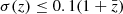 .
.
3. Network and training procedure
3.1. Network input
For each galaxy, a N × 64 × 64 pixel data cube was created with a subtracted background. N is the number of bands (five for SDSS and CFHTLS, six or nine for HSC-Deep). Images in the data cube were sorted in ascending order of wavelength (e.g., ugriz).
The network takes as input a batch of datacubes. Given the wide range of pixel values, the P19 dynamic range compression, xc was applied to each image, x, defined as  . Additionally, each band was center-reduced using all the training objects. This ensures a more robust and efficient training.
Following P19, we also included as an input the galactic reddening excess, E(B − V), as the network had no information regarding the location of the sources. The E(B − V) value was appended to the compressed nonspatial latent representation, helping to break the degeneracy between dust reddening and redshift (i.e., P19).
3.2. The baseline architecture
As a benchmark, we used a network architecture inspired by P19 and presented by Treyer et al. (2024), which currently delivers the best precision for the SDSS MGS dataset (Table 2). The network consists of two convolutional layers followed by multiple sequential inception blocks (inspired by Szegedy et al. 2015). Each inception block is composed of convolutional layers, with different kernel sizes, which capture patterns at different resolutions. On all layers, a ReLU activation function (Nair & Hinton 2010) was used, with the exception of the first and second layers where a PReLU (He et al. 2015) and a hyperbolic tangent function were employed, respectively, to reduce the signal dynamic range. At the end of the sequential blocks, valid padding was applied, reducing the information to 96 one-by-one feature maps. Finally, sequential fully connected layers were employed to produce the classification and regression outputs.
Performance comparison of different deep learning networks on the SDSS MGS (r ≤ 17.8).
3.3. Network output
The redshift estimation task has been treated using either a regression or a classification method. When a regression method is adopted, the network is trained by minimizing a loss function, for example the mean absolute error (MAE) or the root mean squared error (RMSE) between the predicted and true redshifts (Dey et al. 2022; Schuldt et al. 2021).
Alternatively, it can be treated using a classification method, as in P19 and in this work, and also in other kinds of applications (Rothe et al. 2018; Stöter et al. 2018; Rogez et al. 2017). We discretized the redshift space into narrow, mutually exclusive Nb redshift bins. The network was trained to classify each galaxy into the correct redshift bin through the optimization of the softmax cross-entropy (a strictly proper loss function). Gneiting & Raftery (2007) show that its correct minimization guarantees convergence on the true conditional probability.
The outputs of our nonlinear, complex-enough classification network (after the application of the softmax activation function) are positive and normalized scores distributed over the predefined redshift bins. We consider them to be estimators of the true conditional probability of the redshift belonging to a specific bin (LeCun et al. 2015; Krizhevsky et al. 2017; Szegedy et al. 2015), which is, in turn, an approximation of the true redshift probability density function. Consequently, we refer to the network classification output as a redshift probability distribution (PDF).
In Appendix A, we show the performance obtained with models based on regression and/or classification methods using two different training sets. We find that the classification model outperforms the regression model. Additionally, we obtain a slight improvement by combining the classification and regression losses. In all subsequent experiments, we adopted this mixed scheme.
3.4. Network Training Protocol
We used an ADAM optimizer (Kingma & Ba 2014) and a batch size of 32 datacubes to train our network. Data augmentation was applied with random flips and rotations of the images (90° step).
The models were trained by simultaneously optimizing the cross-entropy loss function for the classification module and the MAE for the regression module. For a source, s, with a spectroscopic redshift, zspec, the loss function is the sum of these two loss functions:
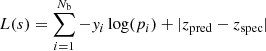 (1)
(1)
where Nb is the number of redshift classes, yi the classification label of the redshift bin i (1 for the bin containing zspec, 0 for the other bins), pi the estimation for the class, i, produced by the classification module, and zpred the regression estimate.
For a given training set, the database was split into five cross-validation samples. Each cross-validation sample (20%) was used as a test sample, while the remaining four (80%) were used for training. This guaranteed that each galaxy appeared once in the test sample. We used ensemble learning (Goodfellow et al. 2016) by running each training configuration several times with weights randomly initialized and the training set randomly shuffled: three times for the HSC and CFHTLS datasets and five times for the SDSS dataset (for comparison with other published works). The final PDF is the average of the outputs of the trained models.
All the results presented in the following sections are limited to i ≤ 24.
4. Multimodality for redshift estimation
A key component of redshift estimation is the correlations between different bands covering different spectral domains. SED fitting techniques and machine learning algorithms exploit the flux ratios between bands. CNNs are able to capture correlations between different channels directly from the images and to extract spatially correlated patterns. In a classical CNN architecture, each kernel of the first convolution layer combines all the channels to produce one feature map (see Fig. 3 in P19).
Multimodality is commonly used to train a network with multiple kinds of input data (i.e., images, audio, text) (Ngiam et al. 2011; Hou et al. 2018). Multiple input streams are incorporated into the network, processed in parallel, and combined at a later stage (Hong et al. 2020). This allows for better feature extraction from each modality.
In the present work, we used multimodality to analyze subsets of bands separately before combining their outputs. In the following, we introduce our formalism for the multimodal configuration, the modifications to the network architecture, and the key hyper-parameters involved in such networks.
4.1. Modalities
The images were sorted in ascending order of wavelength. The size of a modality refers to the number of bands it contains, while the order refers to the proximity of the bands. First-order modalities use adjacent bands, second-order modalities use bands separated by one band, third-order modalities use bands with a gap of two bands, etc. Table C.2 details the modalities of the first, second, and third orders for the ugrizyjhk bands.
4.2. Network architecture
We adopted a flexible network architecture to incorporate the multimodalities. As illustrated in Fig. 1, we defined two main parts:
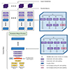 |
Fig. 1. Generic architecture of the multimodality network. The number of parallel blocks is contingent on the number of modalities. The depth of both the parallel and common blocks will be determined by the type of fusion being implemented (early, middle, or late fusion); however, it is important to note that the total network depth is fixed at eight (each modality will go through eight inception blocks in total). The same goes for the average pooling layers; they are performed consistently through the different architectures, before the 1st, 4th, and 6th inception blocks and the last one after the valid padding convolution layers. The baseline model without the multimodality approach represents a special case, where all the image bands are grouped into a single modality. The fixed depth allows for a standardized comparison between the different experiments. |
– Parallel blocks: for each input modality, we defined an independent module at the start of the network. It consists of successive inception blocks sized according to the size of the modality.
– Common block: it combines the outputs of the parallel blocks and proceeds with its own architecture detailed in Fig. 1.
The depth of the parallel and common blocks depend on the type of fusion used as described in the next subsection. However, we limited the total network depth to eight inception blocks and the pooling layers were performed at fixed depths (before the 1st, 4th, and 6th inception blocks). The baseline architecture presented in Sect. 3.2 can be obtained within the current framework by considering only one modality containing all the bands. In the following we use “baseline” and “baseline single modality” interchangeably.
4.3. Fusion
The stage of fusion, in which the parallel processed modalities are combined, is the last key factor to consider. It determines how much network processing is allocated to feature extraction from each modality and how much is assigned to combining those features for redshift estimation. We considered three stages (Hong et al. 2020). First, early fusion where the features from each modality were fused after two parallel inception blocks, prior to passing through six common inception blocks. Second, middle fusion where modalities were combined after four parallel inception blocks, followed by four common blocks. Lastly, late fusion where modalities were combined after six inception blocks, followed by two common blocks.
We tested two methods of fusing the feature maps from the different modalities: simple concatenation and cross-fusion. A cross-fusion module consists of a set of parallel inception blocks, each processing modalities one by one (hence cross) for improved feature blending. The cross-fused feature maps pass through a common convolution layer prior to being concatenated (Hong et al. 2020).
5. Experiments
5.1. Metrics and point estimates
To evaluate the photometric redshift performance between the different experiments, three metrics were considered based on the normalized residuals, Δz = (zphot − zspec)/(1 + zspec) (P19):
– the MAD (median absolute deviation), σMAD = 1.4826 × Median(|Δz − Median(Δz)|)
– the fraction of outliers, η (%), with |Δz|≥0.05 for the SDSS or 0.15 for the other datasets.
– the bias, ⟨Δz⟩=Mean(Δz).
We chose the median of the output PDF as the point estimate, zphot. However this choice was not critical as we are interested in the relative performance of the various experiments.
5.2. Multimodality configurations
To evaluate the impact of the three variable ingredients of our multimodal approach, we used the HSC Deep Imaging Survey dataset (Sect. 2.3), as it covers the widest range of magnitude and redshift and has the largest number of photometric bands. We ran experiments with different multimodal configurations in order to determine: the most efficient stage of fusion, the best fusion type (cross-fusion or simple concatenation), the optimal modality size, and the optimal modality order.
5.2.1. Stage and type of fusion
We conducted four experiments: early, middle, and late fusion with concatenation fusion, and an early cross-fusion scenario, assuming size two and first- and second-order modalities.
The resulting MADs as a function of the magnitude and redshift are shown in Fig. 2 and compared to the baseline, single-modality model. Error bars were defined as the standard deviation between the metrics of the five validation folds. Early and middle fusions provide the most significant improvement, with early fusion slightly outperforming middle fusion. The performance of the early concatenation fusion is similar to the early cross-fusion scheme while being more computationally efficient. Thus, we proceeded with concatenation fusion for the other experiments.
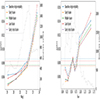 |
Fig. 2. MAD of the redshift estimation as a function of magnitude (i band, left panel) and spectroscopic redshift (right panel) for different types of fusion, compared to the baseline (single modality) model for the HSC 9-band dataset. The gray histograms represent the magnitude and redshift distributions, the horizontal lines show the mean MAD, and the error bars represent the standard deviation between the five validation folds. The data were split into eight x-axis bins containing the same number of objects, each point representing the center of the bin. |
Additionally, we tested very early fusion (where fusion occurs after the two initial convolutions and one inception block) and extremely early fusion (fusion after just two convolutions). Results reported in Fig. B.4 show that early fusion obtains the best precision followed by very early fusion then extremely early fusion.
5.2.2. Size of modalities
We varied the size of the modalities from one to five, assuming first-order and early fusion. The MADs are presented in Fig. 3 as a function of magnitude and redshift. Adopting a size of two or more significantly and similarly improves the performance over the baseline. This confirms our initial hypothesis that processing subsets of bands in parallel prior to merging information helps the network to capture inter-band correlations.
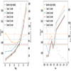 |
Fig. 3. Same as Fig. 2 but for early fusion, first-order modality models with a different number of bands for each modality, compared to the baseline model. |
By contrast, single-band modalities perform similarly to the baseline at faint magnitudes and worse at bright magnitudes. The network may have more difficulties extracting inter-band correlation information, in this case not available until the modalities were merged within the network.
To further investigate these results, we analyzed the impact of modalities of sizes two and four under early, middle, and late fusion, as shown in Fig. 4. We can observe the relatively minor impact of the modality size under the three different configurations. We conclude that the impact of modality size does not depend on the stage of fusion.
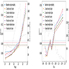 |
Fig. 4. Same as Fig. 2 but for modalities of size two and four using the three different stages of fusion, compared to the baseline model. |
5.2.3. Order of modalities
Here we examine the impact of modalities based on the wavelength closeness of their bands. Assuming two-band modalities and early fusion, we tested four combinations of orders: first; first and second; first, second, and third; and finally second and third orders (the different orders are detailed in Table C.2).
As illustrated in Fig. 5, we find that experiments that included first-order modalities performed optimally. The experiment using only second and third orders was comparable to the baseline, showing that the network was not able to extract additional relevant inter-band correlation information that could outperform the baseline. These results are in line with expectations, as adjacent bands express with the highest resolution the color information directly related to redshift estimation.
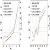 |
Fig. 5. Same as Fig. 2 but for different combinations of orders within 2-band modalities and using early fusion, compared to the baseline model. |
6. Results
Based on the above experiments, we evaluated the multimodal approach using two-band, first-order modalities and performed cross-validations on different datasets.
The SDSS MGS dataset (r ≤ 17.8) provides a benchmark to compare our work with other deep learning redshift estimates (P19; Dey et al. 2022; Hayat et al. 2021) and with the baseline model (Treyer et al. 2024). Results reported in Table 2 show that the multimodal approach outperforms all previous works both in terms of the MAD and the outlier fraction, while not worsening the baseline bias.
We compared the multimodal network with the baseline of the CFHTLS (five bands) and HSC (six and nine bands). Additionally, we tested the network trained on the HSC nine bands on the low-resolution spectroscopic samples 3DHST and PRIMUS and on the high-quality photometric redshift COSMOS2020. The metrics are reported in Table 3. We also report the relative gain or loss defined as follows:
 (2)
(2)
Impact of multimodality on different datasets.
where MB and MM are, respectively, the baseline and multimodality values of a given metric, M. Finally, we estimated the statistical significance of the differences in metrics (MB − MM) using the paired bootstrap test detailed in Appendix D. The computed pvalues are reported in Table 3, with statistically significant differences under a 5% risk threshold highlighted in green.
The results in Table 3 show that the multimodal approach offers statistically significant improvements of the MAD, ranging from 2% to 10%, across all datasets. In the case of 3DHST, the difference is significantly under a 7% risk threshold. Similar improvements are also observed in the outlier fractions, ranging from 4% to 30%. However, the improvements in the HSC nine and six bands and the 3DHST datasets were not statistically significant under a 5% risk threshold. Regarding the bias, the baseline approach performs better on the HSC nine bands and CFHTLS, but with no significant difference. The two-band, first-order setting achieves these results while being only 1.2 times slower than the baseline.
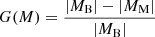
We investigated the relation between the impact multimodality and the number of bands. Figure 6 illustrates the multimodality gains compared to the baseline when training the models with different band combinations, specifically grizy, ugrizy, ugrizyj, ugrizyjh, and ugrizyjhk, using the HSC nine-band subset. We can see that the impact of multimodality on the MAD becomes more pronounced as more bands are incorporated into the training.
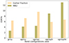 |
Fig. 6. Comparison of the multimodality gain, G(M), using 5, 6, 7, 8, and 9 bands for the MAD and the outlier fraction on the HSC nine-band dataset. |
Its effect on the outlier fraction is less conclusive, as it does not exhibit a consistent pattern with the increasing number of bands.
In conclusion, our experiments show that the multimodality approach offers a statistically significant improvement in the precision of the redshift estimation. This is observed in both the MAD and the outlier fraction across all datasets. The impact is less conclusive for the mean bias.
7. Discussions
7.1. Dependence on network architecture
We evaluated the integration of multimodality in three additional network architectures: a five-layer CNN, a ten-layer CNN, and a 21-layer CNN. The impact of multimodality on the MAD of redshift estimates for these architectures, as well as the inception baseline, is depicted in Fig. 7. The results show a consistent improvement when multimodality is incorporated. Its impact was more substantial in the deeper networks compared to the shallower five-convolution-layer network. We conclude that the effectiveness of multimodality is enhanced when the network architecture is sufficiently deep. Finally, we note that these results are unrelated to the number of network parameters, as shown in Appendix C.
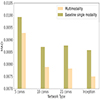 |
Fig. 7. Comparison of the multimodality impact on the MAD of the redshift estimation in the HSC 9-band dataset for 4 different network architectures. |
7.2. Dependence on training set size
We examined the effect of multimodality for various sizes of training set using the HSC nine-band dataset. Figure 8 presents the results when training on 40%, 60%, 80%, and 100% of the training set. The results show that the multimodality improvement relative to the baseline remains consistent regardless of the training set size. We conclude that the effectiveness of multimodality is independent of the number of training objects.
 |
Fig. 8. Comparison of the multimodality impact on the MAD of the redshift estimation in the HSC 9-band dataset for four different sizes of the training set. |
7.3. Multimodality impact on training
The positive impact of multimodality can have different explanations. The most intuitive interpretation is that each parallel block that processes a subset of the input bands specializes in extracting information from the correlations between those bands, ultimately allowing the network to capture more relevant information than the baseline model.
Alternatively, noise may be present in the correlations between all the bands, causing an overfit. This noise would not have a consistent relation with the redshift but the network could map it to the specific redshifts of the training sources, allowing it to optimize the training loss at the expense of extracting more general features. This would result in a suboptimal performance on the validation set. Unlike the baseline, the multimodal network would avoid over-fitting this noise as the correlations between all the bands are not directly available, and so this optimization path would be more difficult to attain.
To investigate which of these two mechanisms better explains the observed gain, we designed the following experiment using the HSC nine-band dataset: we added a new modality containing all nine images to the existing modalities of the multimodal network. If the noise present in the correlation between the bands, which is preserved in the added modality, offers the easiest optimization path and facilitates over-fitting, we would expect the performance to degrade back to the baseline model. If, on the other hand, the benefit of multimodality arises from improved extraction of information, the additional modality should have little impact on the performance.
The results presented in Fig. 9 point to the latter option. We conclude that the multimodality approach gains from extracting more information rather than from reducing over-fitting.
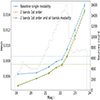 |
Fig. 9. MAD of the redshift estimation for two-band, first-order modalities with and without an additional modality containing all the bands, compared to the baseline model. |
7.4. Modality dropout
In order to study the impact of specific inter-band correlations on redshift estimation, we used a specific type of dropout technique, whereby the output of a given modality was entirely dropped, allowing us to weigh its relative importance on network performance. We aimed to study the impact of the correlations between each two bands and not necessarily the bands themselves.
To do so, we trained a network with two-band, first-order modalities and nine single-band modalities, to guarantee that no information was lost in the test phase when a two-band modality was dropped. During the training phase, we randomly dropped zero to five modalities for each batch, while during the test, we consistently dropped one specific modality.
Figure 10 shows how the test MAD is affected as a function of redshift. The models are ranked according to their impact on the mean MAD value. We also show for comparison the baseline model, our reference multimodal model, and the multimodal model trained with modality dropouts, but tested with no modality dropped. The results can be summarized as follows:
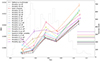 |
Fig. 10. Evolution of the MAD as a function of redshift for the multimodal model with one modality dropped at a time. All the single-band modalities dropped are shown with gray lines as they show similar performances. We also include, for comparison, the baseline model (single modality, dash-dotted cyan line), the reference multimodal model (dash-dotted black line), and the multimodal model trained with dropout but with no modality dropped in the test (dash-dotted dark red line). Finally, we have the different two-band modalities dropped one at a time. Labels on the left panel are ranked according to their mean MAD. The gray histogram shows the redshift distribution of the HSC nine-band test sample. The test objects are evenly distributed between the line points, which are slightly shifted on the x axis for better visual distinctiveness. The horizontal lines on the right represent the mean MAD of each experiment. |
– The network trained with dropouts but tested without performs similarly (marginally lower) to the reference multimodal model. This reflects how the classical model keeps a good level of generalization.
– When dropping only one single-band modality, the results are also very close to the reference multimodal model, whichever band is dropped. This shows that the network focuses more on the two-band modalities, as we might expect.
– When dropping a two-band modality, the impact is very dependant on which one is dropped. Modalities with optical bands, g_r and r_i, are overall the most important, with noticeable trends with redshift.
The blue modality, u_g, is critical at low redshifts, z ≤ 0.5, while j_h, i_z, and z_y are more important at high redshifts, z ≥ 1.
To conclude, the modality dropout test allows us to confirm that our multimodal model retains a good level of generalization and to highlight the importance of specific pairs of bands at different redshifts, as do SED fitting methods but with much better accuracy.
8. Conclusion
We introduce multimodality as a novel approach to redshift estimation in the framework of supervised deep learning. The input consists of galaxy images in several broadband filters, labeled with a spectroscopic redshift. Subsets of bands (modalities) are first processed separately in parallel. Their respective feature maps are then combined at an appropriate stage in the network and fed to a common block. We find that this technique enhances the extraction of color information independently of the network number of parameters and that it significantly improves the redshift precision for various datasets covering a range of characteristics (depth, sky coverage, resolution). In particular, our approach achieves new state-of-the-art results for the widely used SDSS MGS dataset.
We explored modalities of different sizes and different wavelength proximity with different stages of fusion. We conclude that the early fusion of modalities composed of two adjacent bands offer the best results with minimal complexity.
Like other CNNs, our multimodal network fully exploits the information present at the pixel level but the prior parallel processing of bicolor modalities captures additional color information that improves its outcome. We find that the improvement in photometric redshift precision is statistically significant, does not depend on a specific CNN architecture, and increases with the number of photometric filters available. This scheme, combined with a modality dropout test, allows us to highlight the impact of individual colors on the redshift estimation as a function of redshift.
Future work will focus on leveraging the advancements made in this study to produce redshifts for the entire HSC dataset. This will present a number of challenges, such as domain mismatch between different multiband image acquisition conditions and the scarcity of spectroscopically confirmed redshifts. Despite these challenges, the use of multimodality and other developed deep learning techniques have the potential to provide reliable estimates of photometric redshift, which will deliver valuable insights into the large-scale structure of the universe and the evolution of galaxies.
https://calet.org/2018/10/04/final-cfhtls-terapix-dataset-available-at-calet/
The HSC-Deep survey include also narrowband filters not considered in this work.
Acknowledgments
This work was carried out thanks to the support of the DEEPDIP ANR project (ANR-19-CE31-0023, http://deepdip.net), the Programme National Cosmologie et Galaxies (PNCG) of CNRS/INSU with INP and IN2P3, co-funded by CEA and CNES. This publication makes use of Sloan Digital Sky Survey (SDSS) data. Funding for SDSS-III has been provided by the Alfred P. Sloan Foundation, the Participating Institutions, the National Science Foundation, and the US Department of Energy Office of Science. The SDSS-III web site is http://www.sdss3.org/. SDSS-III is managed by the Astrophysical Research Consortium for the Participating Institutions of the SDSS-III Collaboration including the University of Arizona, the Brazilian Participation Group, Brookhaven National Laboratory, Carnegie Mellon University, University of Florida, the French Participation Group, the German Participation Group, Harvard University, the Instituto de Astrofisica de Canarias, the Michigan State/Notre Dame/JINA Participation Group, Johns Hopkins University, Lawrence Berkeley National Laboratory, Max Planck Institute for Astrophysics, Max Planck Institute for Extraterrestrial Physics, New Mexico State University, New York University, Ohio State University, Pennsylvania State University, University of Portsmouth, Princeton University, the Spanish Participation Group, University of Tokyo, University of Utah, Vanderbilt University, University of Virginia, University of Washington, and Yale University. This publication makes use of the Canada France Hawaii Telescope Legacy Survey (CFHTLS) and CFHT Large Area U-band Deep Survey (CLAUDS), based on observations obtained with MegaPrime/MegaCam, a joint project of CFHT and CEA/IRFU, at the Canada-France-Hawaii Telescope (CFHT) which is operated by the National Research Council (NRC) of Canada, the Institut National des Science de l’Univers of the Centre National de la Recherche Scientifique (CNRS) of France, and the University of Hawaii. This work is based in part on data products produced at Terapix available at the Canadian Astronomy Data Centre as part of the Canada-France-Hawaii Telescope Legacy Survey, a collaborative project of NRC and CNRS. CLAUDS use data from the Hyper Suprime-Cam (HSC) camera. The HSC instrumentation and software were developed by the National Astronomical Observatory of Japan (NAOJ), the Kavli Institute for the Physics and Mathematics of the Universe (Kavli IPMU), the University of Tokyo, the High Energy Accelerator Research Organization (KEK), the Academia Sinica Institute for Astronomy and Astrophysics in Taiwan (ASIAA), and Princeton University. Funding was contributed by the FIRST program from Japanese Cabinet Office, the Ministry of Education, Culture, Sports, Science and Technology (MEXT), the Japan Society for the Promotion of Science (JSPS), Japan Science and Technology Agency (JST), the Toray Science Foundation, NAOJ, Kavli IPMU, KEK, ASIAA, and Princeton University. CLAUDS is a collaboration between astronomers from Canada, France, and China described in Sawicki et al. (2019) and uses data products from CALET and the Canadian Astronomy Data Centre (CADC) and was processed using resources from Compute Canada and Canadian Advanced Network For Astrophysical Research (CANFAR) and the CANDIDE cluster at IAP maintained by Stephane Rouberol.
References
- Ahumada, R., Prieto, C. A., Almeida, A., et al. 2020, ApJS, 249, 3 [Google Scholar]
- Aihara, H., AlSayyad, Y., Ando, M., et al. 2019, PASJ, 71, 114 [Google Scholar]
- Alam, S., Albareti, F. D., Allende Prieto, C., et al. 2015, ApJS, 219, 12 [Google Scholar]
- Arnouts, S., Cristiani, S., Moscardini, L., et al. 1999, MNRAS, 310, 540 [Google Scholar]
- Baldry, I. K., Liske, J., Brown, M. J. I., et al. 2018, MNRAS, 474, 3875 [Google Scholar]
- Beck, R., Dobos, L., Budavári, T., Szalay, A. S., & Csabai, I. 2016, MNRAS, 460, 1371 [Google Scholar]
- Benítez, N. 2000, ApJ, 536, 571 [Google Scholar]
- Berg-Kirkpatrick, T., Burkett, D., & Klein, D. 2012, Proceedings of the 2012 Joint Conference on Empirical Methods in Natural Language Processing and Computational Natural Language Learning (Jeju Island, Korea: Association for Computational Linguistics), 995 [Google Scholar]
- Bertin, E. 2006, ASP Conf. Ser., 351, 112 [NASA ADS] [Google Scholar]
- Bertin, E., & Arnouts, S. 1996, A&AS, 117, 393 [NASA ADS] [CrossRef] [EDP Sciences] [Google Scholar]
- Bertin, E., Mellier, Y., Radovich, M., et al. 2002, ASP Conf. Ser., 281, 228 [Google Scholar]
- Boulade, O., Charlot, X., Abbon, P., et al. 2000, in SPIE Conf. Ser., 4008, 657 [NASA ADS] [Google Scholar]
- Bradshaw, E. J., Almaini, O., Hartley, W. G., et al. 2013, MNRAS, 433, 194 [NASA ADS] [CrossRef] [Google Scholar]
- Brammer, G. B., van Dokkum, P. G., & Coppi, P. 2008, ApJ, 686, 1503 [Google Scholar]
- Carliles, S., Budavári, T., Heinis, S., Priebe, C., & Szalay, A. S. 2010, ApJ, 712, 511 [NASA ADS] [CrossRef] [Google Scholar]
- Chen, Y., Li, C., Ghamisi, P., Jia, X., & Gu, Y. 2017, IEEE Geosci. Remote Sens. Lett., 14, 1253 [CrossRef] [Google Scholar]
- Coil, A. L., Blanton, M. R., Burles, S. M., et al. 2011, ApJ, 741, 8 [Google Scholar]
- Collister, A. A., & Lahav, O. 2004, PASP, 116, 345 [NASA ADS] [CrossRef] [Google Scholar]
- Cool, R. J., Moustakas, J., Blanton, M. R., et al. 2013, ApJ, 767, 118 [NASA ADS] [CrossRef] [Google Scholar]
- Csabai, I., Dobos, L., Trencséni, M., et al. 2007, Astron. Nachr., 328, 852 [NASA ADS] [CrossRef] [Google Scholar]
- Dalton, G. B., Caldwell, M., Ward, A. K., et al. 2006, in SPIE Conf. Ser, 6269, 62690X [NASA ADS] [Google Scholar]
- Dark Energy Survey Collaboration (Abbott, T., et al. ) 2016, MNRAS, 460, 1270 [Google Scholar]
- de Jong, J. T. A., Kuijken, K., Applegate, D., et al. 2013, The Messenger, 154, 44 [NASA ADS] [Google Scholar]
- Desprez, G., Picouet, V., Moutard, T., et al. 2023, A&A, 670, A82 [NASA ADS] [CrossRef] [EDP Sciences] [Google Scholar]
- Dey, B., Andrews, B. H., Newman, J. A., et al. 2022, MNRAS, 515, 5285 [NASA ADS] [CrossRef] [Google Scholar]
- Drinkwater, M. J., Byrne, Z. J., Blake, C., et al. 2018, MNRAS, 474, 4151 [Google Scholar]
- Efron, B., & Tibshirani, R. J. 1994, An Introduction to the Bootstrap (CRC Press) [Google Scholar]
- Emerson, J. P., Sutherland, W. J., McPherson, A. M., et al. 2004, The Messenger, 117, 27 [NASA ADS] [Google Scholar]
- Garilli, B., McLure, R., Pentericci, L., et al. 2021, A&A, 647, A150 [NASA ADS] [CrossRef] [EDP Sciences] [Google Scholar]
- Gneiting, T., & Raftery, A. E. 2007, J. Am. Stat. Assoc., 102, 359 [CrossRef] [Google Scholar]
- Goodfellow, I., Bengio, Y., & Courville, A. 2016, Deep Learning (MIT Press) [Google Scholar]
- Hayat, M. A., Stein, G., Harrington, P., Lukić, Z., & Mustafa, M. 2021, ApJ, 911, L33 [NASA ADS] [CrossRef] [Google Scholar]
- He, K., Zhang, X., Ren, S., & Sun, J. 2015, Proceedings of the IEEE International Conference on Computer Vision, 1026 [Google Scholar]
- Hong, D., Gao, L., Yokoya, N., et al. 2020, IEEE Trans. Geosci. Remote Sens., 59, 4340 [Google Scholar]
- Hou, J.-C., Wang, S.-S., Lai, Y.-H., et al. 2018, IEEE Trans. Emerg. Topics. Comput. Intell., 2, 117 [CrossRef] [Google Scholar]
- Hudelot, P., Cuillandre, J. C., Withington, K., et al. 2012, VizieR Online Data Catalog:II/317 [Google Scholar]
- Ilbert, O., Arnouts, S., McCracken, H. J., et al. 2006, A&A, 457, 841 [NASA ADS] [CrossRef] [EDP Sciences] [Google Scholar]
- Ivezić, Ž., Kahn, S. M., Tyson, J. A., et al. 2019, ApJ, 873, 111 [Google Scholar]
- Jarvis, M. J., Bonfield, D. G., Bruce, V. A., et al. 2013, MNRAS, 428, 1281 [Google Scholar]
- Kingma, D. P., & Ba, J. 2014, arXiv e-prints [arXiv:1412.6980] [Google Scholar]
- Koehn, P. 2004, Proceedings of the 2004 Conference on Empirical Methods in Natural Language Processing (Barcelona: Association for Computational Linguistics), 388 [Google Scholar]
- Krizhevsky, A., Sutskever, I., & Hinton, G. E. 2017, Commun. ACM, 60, 84 [CrossRef] [Google Scholar]
- Laureijs, R., Amiaux, J., Arduini, S., et al. 2011, arXiv e-prints [arXiv:1110.3193] [Google Scholar]
- LeCun, Y., Bengio, Y., & Hinton, G. 2015, Nature, 521, 436 [Google Scholar]
- Lee, K.-G., Krolewski, A., White, M., et al. 2018, ApJS, 237, 31 [Google Scholar]
- Le Fèvre, O., Cassata, P., Cucciati, O., et al. 2013, A&A, 559, A14 [Google Scholar]
- Le Fèvre, O., Tasca, L. A. M., Cassata, P., et al. 2015, A&A, 576, A79 [Google Scholar]
- Lilly, S. J., Le Fèvre, O., Renzini, A., et al. 2007, ApJS, 172, 70 [Google Scholar]
- Ma, L., Lu, Z., Shang, L., & Li, H. 2015, Proceedings of the IEEE International Conference on Computer Vision, 2623 [Google Scholar]
- Masters, D. C., Stern, D. K., Cohen, J. G., et al. 2019, ApJ, 877, 81 [Google Scholar]
- McCracken, H. J., Milvang-Jensen, B., Dunlop, J., et al. 2012, A&A, 544, A156 [NASA ADS] [CrossRef] [EDP Sciences] [Google Scholar]
- McLure, R. J., Pearce, H. J., Dunlop, J. S., et al. 2013, MNRAS, 428, 1088 [NASA ADS] [CrossRef] [Google Scholar]
- Miyazaki, S., Komiyama, Y., Kawanomoto, S., et al. 2018, PASJ, 70, S1 [NASA ADS] [Google Scholar]
- Momcheva, I. G., Brammer, G. B., van Dokkum, P. G., et al. 2016, ApJS, 225, 27 [Google Scholar]
- Nair, V., & Hinton, G. E. 2010, Proceedings of the 27th International Conference on Machine Learning (ICML-10), 807 [Google Scholar]
- Newman, J. A., Cooper, M. C., Davis, M., et al. 2013, ApJS, 208, 5 [Google Scholar]
- Ngiam, J., Khosla, A., Kim, M., et al. 2011, Proceedings of the 28th international Conference on Machine Learning (ICML-11), 689 [Google Scholar]
- Pasquet, J., Bertin, E., Treyer, M., Arnouts, S., & Fouchez, D. 2019, A&A, 621, A26 [NASA ADS] [CrossRef] [EDP Sciences] [Google Scholar]
- Qian, K., Zhu, S., Zhang, X., & Li, L. E. 2021, Proceedings of the IEEE/CVF Conference on Computer Vision and Pattern Recognition, 444 [Google Scholar]
- Regnault, N., Conley, A., Guy, J., et al. 2009, A&A, 506, 999 [NASA ADS] [CrossRef] [EDP Sciences] [Google Scholar]
- Rogez, G., Weinzaepfel, P., & Schmid, C. 2017, Proceedings of the IEEE Conference on Computer Vision and Pattern Recognition, 3433 [Google Scholar]
- Rothe, R., Timofte, R., & Van Gool, L. 2018, Int. J. Comput. Vision, 126, 144 [CrossRef] [Google Scholar]
- Sawicki, M., Arnouts, S., Huang, J., et al. 2019, MNRAS, 489, 5202 [NASA ADS] [Google Scholar]
- Schlegel, D. J., Finkbeiner, D. P., & Davis, M. 1998, ApJ, 500, 525 [Google Scholar]
- Schuldt, S., Suyu, S. H., Cañameras, R., et al. 2021, A&A, 651, A55 [NASA ADS] [CrossRef] [EDP Sciences] [Google Scholar]
- Scodeggio, M., Guzzo, L., Garilli, B., et al. 2018, A&A, 609, A84 [NASA ADS] [CrossRef] [EDP Sciences] [Google Scholar]
- Skelton, R. E., Whitaker, K. E., Momcheva, I. G., et al. 2014, ApJS, 214, 24 [Google Scholar]
- Szalay, A. S., Connolly, A. J., & Szokoly, G. P. 1999, AJ, 117, 68 [Google Scholar]
- Szegedy, C., Liu, W., Jia, Y., et al. 2015, Proceedings of the IEEE Conference on Computer Vision and Pattern Recognition, 1 [Google Scholar]
- Treyer, M., Ait-Ouahmed, R., Pasquet, J., et al. 2024, MNRAS, 527, 651 [Google Scholar]
- Stöter, F.-R., Chakrabarty, S., Edler, B., & Habets, E. A. P. 2018, 2018 IEEE International Conference on Acoustics, Speech and Signal Processing (ICASSP), 436 [CrossRef] [Google Scholar]
- Weaver, J. R., Kauffmann, O. B., Ilbert, O., et al. 2022, ApJS, 258, 11 [NASA ADS] [CrossRef] [Google Scholar]
Appendix A: Classification or regression
To study the impact of both classification and regression training strategies, we tested different models on both the HSC nine-band and the CFHTLS datasets using the single modality scheme.
We tested training the model with the regression module using three different losses:
-
the root-mean-square error (RMSE),
-
the mean absolute error (MAE), MAE = mean(|zpred − zspec|)
-
the normalized MAE (NMAE, with the residuals normalized by the value of the label),
We also tested a model trained solely with classification, and one aided by a MAE regression, by combining with equal weight the two loss functions in the training.
The results of these experiments are presented in Table A.1.
Global performances of classification- and regression-based models (see text) for the HSC nine-band and CFHTLS datasets.
For the two datasets, the performances with the regression appear to depend on the choice of the loss function, with the normalized MAE leading to the best performances. Overall, the classification-based models outperform the regression ones (especially for the MAD) for both datasets, independently of the depth and number of available bands. It is even slightly improved when the classification is co-optimized with a regression for the HSC dataset (we used the classification module estimation in this case).
In conclusion, we adopted a classification model aided by a regression for all the experiments presented in this work.
Appendix B: Multimodality impact on outlier fraction and bias
We previously detailed the impact of the different multimodal configurations on the MAD metric. Here we show the evolution of the outlier fraction and bias as a function of the i band magnitude and the estimated redshift, zpred. We can see in Figures B.1, B.2, and B.3 that different multimodality configurations only slightly improve the outlier fraction and have little impact on the bias compared to the baseline model.
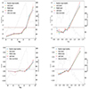 |
Fig. B.1. Comparison of the outlier fraction and bias versus the band i magnitude and predicted redshift of different fusion types and the single modality baseline on the nine-band sources from the HSC dataset |
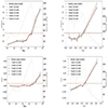 |
Fig. B.2. Same as Fig B.1 but for early fusion, first-order modality models with a different number of bands for each modality and the single modality baseline. |
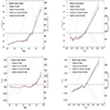 |
Fig. B.3. Same as Fig B.1 but for different modality order combinations for two-band modalities using early fusion and the single modality baseline. |
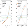 |
Fig. B.4. Same as Fig 2 but for early, very early and extremely early fusion models and the baseline model. |
Appendix C: Configuration details
Table C.1 shows the number of parameters for various experiments. We note that certain multimodal models outperformed the baseline while having a lower number of parameters, like the two-band first-order modalities with early fusion. Additionally, other models with a higher number of parameters, such as the five-band first-order modalities with early fusion, also showed improved performance. These results reinforce our conclusion that the effectiveness of the multimodal approach relies not on the number of parameters but rather on its superior capacity to extract relevant information.
Trainable parameter count for various models
Table C.2 details the composition of first-, second-, and third-order modalities, and the sizes of two, three, and four bands per modality when using the ugrizyjhk bands.
Modality bands for various configurations
Appendix D: Paired bootstrap test
To assess the statistical significance of the observed difference between the baseline and the multimodal approaches, we used the paired bootstrap significance test introduced by Efron & Tibshirani (1994) and frequently used in the field of natural language processing (Berg-Kirkpatrick et al. 2012; Koehn 2004). It is a nonparametric hypothesis test with no assumption about the distribution of the data. For a given dataset, D, we defined
 (D.1)
(D.1)
where MM(D) and MB(D) are the metrics of the multimodal and the baseline model for the dataset, D, respectively. We first assumed that MM is, contrary to what we believe, equal or worse than MB. This is known as the null hypothesis, H0. Next, for a given dataset, Dtest, we estimated the likelihood, pvalue(Dtest), of observing, under H0 and on a new dataset, D, a metric gain, δM(D), equal to or better than δM(Dtest), so that
 (D.2)
(D.2)
A low pvalue(Dtest) suggests that observing δ(Dtest) is unlikely if H0 were true, so we can reject H0 and conclude that the metric gain, δ(Dtest), of MM compared to MB is significant and not just a random fluke.
The pvalue(Dtest) is hard to compute and must be approximated as we don’t have new datasets to test on, so we used the paired bootstrap method to simulate this. We sampled from the test set, with replacement, K, same-size samples as the test set, on which δ(Dtest) was computed. We refer to these samples as bootstrapped samples.
Naively, we may think that we should compute the frequency of δ(Dbootstrapped)≥δ(Dtest) over the K samples as an approximation of pvalue(Dtest). However, these samples aren’t suitable for our null hypothesis H0 since they were sampled from the test set, causing their average δ(Dbootstrapped) to be around δ(Dtest), contrary to what H0 requires. Because H0 assumes that the initially observed difference, δ(Dtest), is due to a random fluke, the solution is to shift the δ(Dbootstrapped) distribution by this value, so we obtain
 (D.3)
(D.3)
The results reported in Table. 3 were obtained with a significance test assuming K = 104.
Fig. D.1 illustrates two cases for the HSC nine-band dataset: the left panel shows the distributions of the MAD of the bootstrapped samples, where the performance gain is significant; the right panel shows the distributions of the outlier fractions where the gain is not significant under a 5% risk threshold. The green histogram is the original distribution that does not satisfy H0. The red histogram is the shifted one that satisfies H0. The blue line represents the difference initially observed on the test dataset, δ(Dtest), and the pvalue(Dtest) corresponds to the fraction of the red histogram exceeding this value.
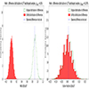 |
Fig. D.1. Distribution of the MAD and outlier fraction differences for a K = 104 paired bootstrap test to assess the significance of the difference between MM and MB on the HSC nine-band test dataset. |
All Tables
Performance comparison of different deep learning networks on the SDSS MGS (r ≤ 17.8).
Global performances of classification- and regression-based models (see text) for the HSC nine-band and CFHTLS datasets.
All Figures
|
Fig. 1. Generic architecture of the multimodality network. The number of parallel blocks is contingent on the number of modalities. The depth of both the parallel and common blocks will be determined by the type of fusion being implemented (early, middle, or late fusion); however, it is important to note that the total network depth is fixed at eight (each modality will go through eight inception blocks in total). The same goes for the average pooling layers; they are performed consistently through the different architectures, before the 1st, 4th, and 6th inception blocks and the last one after the valid padding convolution layers. The baseline model without the multimodality approach represents a special case, where all the image bands are grouped into a single modality. The fixed depth allows for a standardized comparison between the different experiments. |
| In the text | |
|
Fig. 2. MAD of the redshift estimation as a function of magnitude (i band, left panel) and spectroscopic redshift (right panel) for different types of fusion, compared to the baseline (single modality) model for the HSC 9-band dataset. The gray histograms represent the magnitude and redshift distributions, the horizontal lines show the mean MAD, and the error bars represent the standard deviation between the five validation folds. The data were split into eight x-axis bins containing the same number of objects, each point representing the center of the bin. |
| In the text | |
|
Fig. 3. Same as Fig. 2 but for early fusion, first-order modality models with a different number of bands for each modality, compared to the baseline model. |
| In the text | |
|
Fig. 4. Same as Fig. 2 but for modalities of size two and four using the three different stages of fusion, compared to the baseline model. |
| In the text | |
|
Fig. 5. Same as Fig. 2 but for different combinations of orders within 2-band modalities and using early fusion, compared to the baseline model. |
| In the text | |
|
Fig. 6. Comparison of the multimodality gain, G(M), using 5, 6, 7, 8, and 9 bands for the MAD and the outlier fraction on the HSC nine-band dataset. |
| In the text | |
|
Fig. 7. Comparison of the multimodality impact on the MAD of the redshift estimation in the HSC 9-band dataset for 4 different network architectures. |
| In the text | |
|
Fig. 8. Comparison of the multimodality impact on the MAD of the redshift estimation in the HSC 9-band dataset for four different sizes of the training set. |
| In the text | |
|
Fig. 9. MAD of the redshift estimation for two-band, first-order modalities with and without an additional modality containing all the bands, compared to the baseline model. |
| In the text | |
|
Fig. 10. Evolution of the MAD as a function of redshift for the multimodal model with one modality dropped at a time. All the single-band modalities dropped are shown with gray lines as they show similar performances. We also include, for comparison, the baseline model (single modality, dash-dotted cyan line), the reference multimodal model (dash-dotted black line), and the multimodal model trained with dropout but with no modality dropped in the test (dash-dotted dark red line). Finally, we have the different two-band modalities dropped one at a time. Labels on the left panel are ranked according to their mean MAD. The gray histogram shows the redshift distribution of the HSC nine-band test sample. The test objects are evenly distributed between the line points, which are slightly shifted on the x axis for better visual distinctiveness. The horizontal lines on the right represent the mean MAD of each experiment. |
| In the text | |
|
Fig. B.1. Comparison of the outlier fraction and bias versus the band i magnitude and predicted redshift of different fusion types and the single modality baseline on the nine-band sources from the HSC dataset |
| In the text | |
|
Fig. B.2. Same as Fig B.1 but for early fusion, first-order modality models with a different number of bands for each modality and the single modality baseline. |
| In the text | |
|
Fig. B.3. Same as Fig B.1 but for different modality order combinations for two-band modalities using early fusion and the single modality baseline. |
| In the text | |
|
Fig. B.4. Same as Fig 2 but for early, very early and extremely early fusion models and the baseline model. |
| In the text | |
|
Fig. D.1. Distribution of the MAD and outlier fraction differences for a K = 104 paired bootstrap test to assess the significance of the difference between MM and MB on the HSC nine-band test dataset. |
| In the text | |
Current usage metrics show cumulative count of Article Views (full-text article views including HTML views, PDF and ePub downloads, according to the available data) and Abstracts Views on Vision4Press platform.
Data correspond to usage on the plateform after 2015. The current usage metrics is available 48-96 hours after online publication and is updated daily on week days.
Initial download of the metrics may take a while.