| Issue |
A&A
Volume 650, June 2021
|
|
|---|---|---|
| Article Number | A142 | |
| Number of page(s) | 10 | |
| Section | Interstellar and circumstellar matter | |
| DOI | https://doi.org/10.1051/0004-6361/202140829 | |
| Published online | 21 June 2021 | |
The ionized heart of a molecular disk
ALMA observations of the hyper-compact HII region G24.78+0.08 A1★
1
INAF – Osservatorio Astrofisico di Arcetri,
Largo E. Fermi 5,
50125
Firenze,
Italy
e-mail: This email address is being protected from spambots. You need JavaScript enabled to view it.
2
Centro de Astrobiología (CSIC-INTA),
Ctra. de Ajalvir Km. 4,
Torrejón de Ardoz,
28850
Madrid, Spain
Received:
18
March
2021
Accepted:
29
April
2021
Abstract
Context. Hyper-compact (HC) or ultra-compact H II regions are the first manifestations of the radiation feedback from a newly born massive star. Therefore, their study is fundamental to understanding the process of massive (≥8 M⊙) star formation.
Aims. We employed Atacama Large Millimeter/submillimeter Array (ALMA) 1.4 mm Cycle 6 observations to investigate at high angular resolution (≈0.′′050, corresponding to 330 au) the HC H II region inside molecular core A1 of the high-mass star-forming cluster G24.78+0.08.
Methods. We used the H30α emission and different molecular lines of CH3CN and 13CH3CN to study the kinematics of the ionized and molecular gas, respectively.
Results. At the center of the HC H II region, at radii ≲500 au, we observe two mutually perpendicular velocity gradients, which are directed along the axes at PA = 39° and PA = 133°, respectively. The velocity gradient directed along the axis at PA = 39° has an amplitude of 22 km s−1 mpc−1, which is much larger than the other’s, 3 km s−1 mpc−1. We interpret these velocity gradients as rotation around, and expansion along, the axis at PA = 39°. We propose a scenario where the H30α line traces the ionized heart of a disk-jet system that drives the formation of the massive star (≈20 M⊙) responsible for the HC H II region. Such a scenario is also supported by the position-velocity plots of the CH3CN and 13CH3CN lines along the axis at PA = 133°, which are consistent with Keplerian rotation around a 20 M⊙ star.
Conclusions. Toward the HC H II region in G24.78+0.08, the coexistence of mass infall (at radii of ~5000 au), an outer molecular disk (from ≲4000 au to ≳500 au), and an inner ionized disk (≲500 au) indicates that the massive ionizing star is still actively accreting from its parental molecular core. To our knowledge, this is the first example of a molecular disk around a high-mass forming star that, while becoming internally ionized after the onset of the H II region, continues to accrete mass onto the ionizing star.
Key words: ISM: individual objects: G24.78+0.08 / HII regions / ISM: molecules / masers / techniques: interferometric
Reduced images and datacubes are only available at the CDS via anonymous ftp to cdsarc.u-strasbg.fr (130.79.128.5) or via http://cdsarc.u-strasbg.fr/viz-bin/cat/J/A+A/650/A142
© ESO 2021
1 Introduction
The process of the formation of massive (≥8 M⊙ and ≥104 L⊙) stars is characterized by high mass accretion rates, ≥10−4 M⊙ yr−1 (see, for instance, Tan et al. 2014), and strong radiation feedback from the star once it reaches the zero-age main sequence (ZAMS). This feedback includes both the radiation pressure and photoionization of the circumstellar gas, which is evidenced by the appearance of a hyper-compact (HC; size ≲ 0.01 pc) or ultra-compact (UC; ≲0.1 pc) H II region (Kurtz 2005). The stellar mass for the onset of an H II region depends critically on the geometry and mass accretion rate onto the (proto)star (Hosokawa et al. 2010), and it is predicted to vary in the range 10–30 M⊙. Recent simulations that also account for radiation feedback (Tanaka et al. 2016; Kuiper & Hosokawa 2018) suggest that the formation ofhigh-mass stars, similar to that of low-mass stars, proceeds through a disk-outflow system, in which mass accretion and ejectionare intimately related, until the photoionization and radiation forces yield a progressive broadening of the cavities of the protostellar outflow and eventually quench stellar accretion completely.
The depicted scenario can be much more complicated if the stellar mass is accreted irregularly in time, as is the case for the high-mass young stellar objects (YSOs) S255 NIRS3 (Caratti o Garatti et al. 2017) and NGC 6334I-MM1 (Hunter et al. 2017), which recently underwent a luminosity burst. In this case, as predicted by specific models (Peters et al. 2010b) and observed for several HC or UC H II regions (Galván-Madrid et al. 2008; Franco-Hernández & Rodríguez 2004; Rodríguez et al. 2007), the H II region can flicker on timescales as short as ~ 10 yr owing to rapid changes in its size, which, therefore, becomes an ambiguous indicator of age. A crucial aspect also concerns the photoevaporation of the neutral disk (Hollenbach et al. 1994), whose rate is difficult to estimate since it depends strongly on the disk geometry and (proto)stellar wind structure, which are poorly constrained by observations at the relevant small (~ 100 au) scales.
In the last ten years, the high angular resolution (~ 0.′′1) and sensitivity (≲ 10 μJy) of the Jansky Very Large Array (JVLA) have allowed us to study the properties of the centimeter continuum emission from individual high-mass YSOs. Recent JVLA surveys targeting the earliest stages of massive star formation, from infrared dark clouds to hot molecular cores, have in most cases detected weak and compact radio emission near (within 1000 au of) the YSO, which is generally interpreted in terms of an ionized wind (Moscadelli et al. 2016; Purser et al. 2016, 2021; Rosero et al. 2016; Sanna et al. 2018). For several targets, the elongated and knotty structure of the continuum clearly identifies a radio jet; in a few cases, knots with a negative spectral index (indicative of synchrotron emission) are also observed (Sanna et al. 2019; Rosero et al. 2019). In agreement with the results from the radio continuum, Moscadelli et al. (2019) find that the three-dimensional velocity distribution of the water masers, which trace shocked gas near the YSO, is generally consistent with the predictions for disk winds (DWs) and jets. It is remarkable that the radio luminosity of the ionized winds and jets from massive YSOs is several orders of magnitude below that expected from an optically thin H II region photoionized by a ZAMS star that has a bolometric luminosity equal to that of the YSO (see, for instance, Anglada et al. 2018, their Fig. 8). Instead, the radio luminosities of the observed HC or UC H II regions are distributed close to the optically thin limit (see, for instance, Fig. 18c of Tanaka et al. 2016). These observations indicate that the radio winds and jets are shock-ionized and represent a stage in massive star formation prior to the onset of photoionization and the development of an H II region.
For the past few decades, the kinematics of the ionized gas inside HC or UC H II regions has been investigated with the Very Large Array (VLA; and, more recently, the JVLA) using hydrogen radio recombination lines (RRLs) at centimeter wavelengths. In several objects, these observations discovered large ordered motions across the ionized gas on scales of 100–1000 au, corresponding to infall toward, rotation around, or outflow away from the ionizing star(s) (Keto 2002; Sewiło et al. 2008; Keto & Klaassen 2008; De Pree et al. 2020). The advent of the Atacama Large Millimeter/submillimeter Array (ALMA) has allowed us to observe RRLs of lower quantum numbers, which trace the gas kinematics more reliably because they are less affected by pressure broadening, and achieve much higher sensitivity, to extend the study to a larger sample of weaker H II regions (Klaassen et al. 2018; Rivera-Soto et al. 2020). Moreover, ALMA permits the physical conditions and the kinematics of the molecular gas adjacent to the ionized gas to be determined in unprecedented detail. The discovery of HC or UC H II regions in which the ionized gas undergoes a global motion of infall or rotation suggests that mass accretion onto the star can also proceed after the onset of photoionization, in agreement with the models of “trapped” H II regions (Keto 2003, 2007). Up to now, however, although clear cases of compact ionized rotating structures (size ≲ 100 au) have been reported in the literature (Zhang et al. 2017, 2019; Jiménez-Serra et al. 2020), the corresponding rotation in the molecular gas surrounding the HC or UC H II region on scales of ~ 1000 au has never been observed. The coexistence of both the outer molecular and inner ionized parts of the accretion disk is expected if the massive star inside the H II region is still actively accreting from its parental molecular core, as predicted by the most complete models of massive star formation (Tanaka et al. 2016; Kuiper & Hosokawa 2018).
The high-mass star-forming region G24.78+0.08 (bolometric luminosity of ~ 2 × 10⁵ L⊙ at a distance of 6.7 ± 0.71 kpc) contains a number of molecular cores distributed over ~ 0.1 pc (see Fig. 1). Inside the most prominent molecular core, A1, VLA A-Array (from 21 cm to 7 mm) observations (Beltrán et al. 2007; Cesaroni et al. 2019) have revealed a bright (~ 100 mJy at 1.3 cm) HC (size ≈1000 au) H II region. Beltrán et al. (2006) mapped the core with the VLA B-Array in NH3 and detected red-shifted absorption toward the HC H II region, suggesting mass infall on scales of 5000 au. Moscadelli et al. (2018) observed the HC H II region with ALMA at 1.4 mm during Cycle 2 (2015), achieving an angular resolution of ≈0.′′2 (corresponding to a linear scale of ≈1300 au). The analysisof the H30α line reveals a fast bipolar flow in the ionized gas, covering a range of local standard of rest (LSR) velocities (VLSR) of ≈60 km s−1. The amplitude of the VLSR gradient, 22 km s−1 mpc−1, is one of thehighest observed to date toward HC H II regions. Water and methanol masers are distributed around the HC H II region, and the three-dimensional maser velocities clearly indicate that the ionized gas is expanding at a high speed (≥ 200 km s−1) into the surrounding molecular gas.
The present paper reports on new 1.4 mm ALMA Cycle 6 observations of the G24.78+0.08 region; the angular resolution has improved to ≈0.′′050, corresponding to ≈330 au at the distance of the target. The new ALMA data allow us, for the first time, to map the velocity of the ionized gas, and, at the same time, study the kinematics of the surrounding molecular gas. The ALMA observations are described in Sect. 2. In Sect. 3, we present the main observational results, which are discussed in Sect. 4. Our conclusions are drawn in Sect. 5.
2 ALMA observations
ALMA observed G24.78+0.08 on 2019 July 29 during Cycle 6 while the 12 m array, which included 45 antennas, was in the C43-8 configuration. The baselines ranged from 92 m to 8.5 km, for a maximum recoverable angular scale of 0.′′ 8. The observations lasted ≈90 min, of which ≈47 min were devoted to the target. The flux and bandpass calibrator was the quasar J1924−2914, and the phase calibrator was the quasar J1832−1035.
The systemic velocity of G24.78+0.08, employed for Doppler correction during observations, was Vsys = 111.0 km s−1. Thirteen spectral windows (SPWs) were observed over the frequency range 216.0–237 GHz: one broad (bandwidth of 1.9 GHz) SPW, for sensitive continuum measurement, and twelve narrow (0.23 GHz) SPWs, to achieve high velocity resolution (0.33–0.66 km s−1) for specific spectral lines, such as the CH3CN JK = 12K–11K (K = 0−6) transitions, which are suitable for studying the kinematics and physical conditions of the gas. Data calibration was performed using the pipeline, version “42866M”, for ALMA data analysis in the Common Astronomy Software Applications (CASA; McMullin et al. 2007)package, version 5.6. The image of each SPW (continuum plus line emission) was produced manually using the TCLEAN task with the robust parameter of Briggs (1995) set to 0.5 as a compromise between resolution and sensitivity to extended emission. The clean beams of the resulting images have full width at half maximum (FWHM) major and minor sizes in the range 0.′′ 070–0.′′075 and 0.′′ 049–0.′′052, and positionangles (PAs) ≈ 62°. To map the emission of the ionized gas at high sensitivity, we also produced a naturally weighted image of the H30α line, the most intense and broadest spectral feature of SPW 5. The clean beam of the naturally weighted image has a FWHM of 0.′′ 080 × 0.′′062 and a PA = 75°.
For each SPW, to determine the continuum level of the spectra and subtract it from the line emission, we used STATCONT2 (Sanchez-Monge et al. 2018), a statistical method for estimating the continuum level at each position of the map from the spectral distribution of the intensity at that position. The continuum image of G24.78+0.08 has a 1σ rms noise level of 0.2 mJy beam−1, which is limited by the dynamic range. The 1σ rms noise in a single spectral channel varies in the interval 1–2 mJy beam−1, depending on the considered SPW.
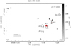 |
Fig. 1 ALMA 2015 and JVLA observations of the high-mass star-forming region G24.78+0.08. The grayscale image shows the ALMA 1.4 mm continuum, with the intensity scale shown to the right of the panel. The black contour is the 7σ threshold of 1.2 mJy beam−1. The continuum emission fragments into distinct cores, labeled following Beltrán et al. (2011). The red contours reproduce the JVLA A-Array 1.3 cm continuum observed by Moscadelli et al. (2018), plotting levels from 0.3 to 16.3 in steps of 4 mJy beam−1. The insets in the lower left and right corners of the plot show the ALMA and JVLA beams, respectively. |
3 Results
3.1 Velocity field in the ionized gas
The velocity map of the ionized gas presented in Fig. 2 (upper panel) reveals a well-defined spatially resolved VLSR gradient, which, across a few thousand au along the SW–NE direction, spans ≈6 km s−1 in velocity.This finding confirms the results from the previous (Cycle 2) lower-angular-resolution (beam FWHM ≈ 0.′′2) ALMA observations by Moscadelli et al. (2018), who discovered a large (ΔVLSR ≈ 60 km s−1) SW-NE oriented (PA = 39°) velocity gradient in the ionized gas at the center of the HC H II region (see Fig. 2, lower panel). In these previous ALMA observations, which could not spatially resolve the HC H II region, the VLSR gradient was obtained from the velocity pattern of the channel peak positions, employing a technique that provides us with relative positions as accurate as ~10 mas (Moscadelli et al. 2018, see their Fig. 8) but does not provide information about the morphology of the emission. With an angular resolution of ≈70 mas, the velocity map from the new ALMA observations (Cycle 6) unveils the spatial distribution of the slower ionized gas.
The upper panel of Fig. 3 shows a less sensitive but higher-angular-resolution (≈58 mas) map of the velocity field of the ionized gas. The mapped area is significantly smaller than that in Fig. 2 (upper panel) and corresponds only to the center of the HC H II region. The velocity of the ionized gas varies regularly with position and is blue- and red-shifted toward the SE and NW, respectively. Taking the pixels of maximum and minimum velocities, we derive a VLSR gradient oriented at PA = 133° and with an amplitude of ≈12 km s−1 across a distance of ≈850 au. The lower panel of Fig. 3 shows the position-velocity (PV) plot of the H30α line along the cut at PA = 133°.
Transitions considered in this work.
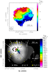 |
Fig. 2 HC H II region. Upper panel: ALMA 2019 data: intensity-weighted velocity (color map) of the H30α emission, obtained from averaging the channel maps produced with a natural weighting of the uv -data. The beam (FWHM 0.′′080 × 0.′′062, with PA = 75°) is shown in the lower left corner. The black contours represent the velocity-integrated intensity of the H30α line, showinglevels from 0.26 to 1.3 in steps of 0.13 Jy beam−1 km s−1. The dashedblack rectangle delimits the field of view shown in the lower panel. Lower panel: ALMA 2015, VLA, and Very Long Baseline Interferometry (VLBI) data. The grayscale image represents the VLA A-Array 7 mm continuum observed by Beltrán et al. (2007). The white triangles and yellow squares mark the VLBI positions of the H2O 22 GHz (Moscadelli et al. 2007) and CH3OH 6.7 GHz masers (Moscadelli et al. 2018), respectively; the area of the symbol is proportional to the logarithm of the maser intensity. The white arrows show the proper motions of the H2O masers, which were first reported and analyzed in Moscadelli et al. (2007). The colored dots give the channel peak positions of the H30α line emissionobtained by Moscadelli et al. (2018) from ALMA data with 0.′′2 resolution; the colors denote the VLSR as indicated to the right of the plot. The dashed black line marks the axis of the spatial distribution of the H30α peaks. |
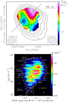 |
Fig. 3 ALMA 2019 data. Upper panel: intensity-weighted velocity (color map) of the H30α emission, obtained from averaging the channel maps produced by weighting the uv -data with the “Briggs” robust parameter set to 0.5. The circular restoring beam has a FWHM size (0.′′ 058) equal to the geometric mean of the FWHM major and minor sizes of the Briggs beam and is shown in the lower left corner. The straight line indicates the direction, at PA = 133°, that connects the pixels of maximum and minimum velocity. The ALMA 1.4 mm continuum is represented with black contours, ranging from 3.2 to 10.6 in steps of 1.1 mJy beam−1. The beam of the continuum map is reported in the lower right corner. Lower panel: color map and white contours showing the PV plot of the H30α line along the cut at PA = 133°. The contour levels range from 4.9 to 24.6 in steps of 4.9 mJy beam−1. The vertical and horizontal white axes denote the positional offset (≈ −0.′′68) and VLSR (≈112 km s−1) of the YSO, respectively. In the lower right corner, the vertical and horizontal yellow error bars indicate the velocity and spatial resolutions, respectively. |
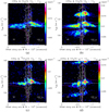 |
Fig. 4 ALMA 2019 data. Each panel presents the combined PV plots, along the cut at PA = 133°, of the H30α emission (white contours; same as Fig. 3, lower panel) and a selected molecular line (color map): CH3CN JK = 123–113 (a); CH3CN JK = 126 –116 (b); 13CH3CN JK = 133–123 (c); and CH3CN v8 = 1 JK,l = 122,1–112,1 (d). Panels b and d: emission of other transitions close in frequency to the selected line. In each panel, the vertical and horizontal white axes denote the positional offset (≈ −0.′′68) and VLSR (≈112 km s−1) of the YSO, respectively. The magenta curve shows the Keplerian velocity profile for a central mass of 20 M⊙. In the lower left corner, the vertical and horizontal white error bars indicate the velocity and spatial resolutions, respectively. |
3.2 Kinematics and physical conditions of the neutral gas
The neutral gas surrounding the HC H II region can be traced by a plethora of molecular lines of different excitations (Moscadelli et al. 2018, see their Table 2 and Figs. 2 and 3); the numerous rotational transitions of CH3CN and associated isotopologs are sufficiently unblended and intense to be used in our study. Table 1 lists the parameters of the lines of CH3CN and 13CH3CN employed in our analysis. To compare the kinematics of the molecular and ionized gas, we constructed PV plots along the direction, at PA = 133° (see Fig. 3), of the VLSR gradient in the ionized gas detected close to the center of the HC H II region. Before producing the PV plot, the emission was averaged across three pixels (that is, 21 mas) in the direction perpendicular to the positional cut. In Fig. 4 we overlay the PV plot of the H30α line with that of various transitions of CH3CN and 13CH3CN with upper level excitation energies ranging between 133 and 596 K.
The physical conditions of the molecular gas can be derived by fitting all the unblended lines of a given molecular species simultaneously. For this purpose, we used the XCLASS (eXtended CASA Line Analysis Software Suite) tool (Möller et al. 2017). This tool models the data by solving the radiative transfer equation in one dimension for an isothermal homogeneous object in local thermodynamic equilibrium (LTE). The fitted quantities are column density, rotation temperature, velocity, line width, and source size. The fit takes the optical depth of the lines into account as well. To determine the physical conditions of the molecular gas as close as possible to the surface of the H II region, we used XCLASS to fit the 13CH3CN JK = 13K–12K, K = 0–5, lines, which offer a good compromise between high signal-to-noise ratio (S/N) and low-to-moderate optical depth. In Fig. 5 we show the fit to the spectrum obtained by averaging the 13CH3CN emission over a circle of 0.′′1 radius around the center of the H II region. The column density, Ncol, and rotational temperature, Trot, of 13CH3CN are found to be  and
and  K. The derived optical depths at the emission peak are 0.12, 0.12, 0.11, 0.18, 0.07, and 0.06 for the K = 0, 1, 2, 3, 4, and 5 lines, respectively.
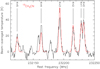 |
Fig. 5 ALMA 2019 data: observed spectrum (black line) of SPW 6 across a frequency range covering the 13CH3CN JK = 13K–12K, K = 0–5, lines. The emission is averaged over a circle of 0.′′1 radius toward the center of the HC H II region. The fit (red histogram) of the 13CH3CN JK = 13K–12K, K = 0–5, lines performed with XCLASS is also reported. |
4 Discussion
4.1 Kinematics of ionized and molecular gas
The velocity maps of the ionized gas presented in Figs. 2 and 3 reveal three distinct velocity components. At the center of the HC H II region, over ≲500 au, we observe two mutually perpendicular VLSR gradients, directed along the axes at PA = 39° and PA = 133°. Remarkably, the velocity gradient directed along the axis at PA = 39° has an amplitude, 22 km s−1 mpc−1, that is much larger than that at PA = 133°, 3 km s−1 mpc−1. At larger radii of a few thousand au, we observe a relatively slow and wide-angle motion of the ionized gas along the SW-NE direction. Since the first two motions occur on similar (small) scales and are mutually perpendicular, and taking their different amplitudes into account, we interpret them in terms of a disk-jet system: the fast motion along the axis at PA = 39° corresponds to the ionized jet; the slower motion corresponds to the rotation of an ionized disk around the same axis. Following this interpretation, and assuming that the VLSR gradient oriented at PA = 133° (spanning ΔV ≈ 12 km s−1 across a distance ΔS ≈ 850 au; see Sect. 3.1) is due to rotation in gravito-centrifugal equilibrium, we derive a central mass  17 M⊙ (where G is the gravitational constant). This value is a lower limit because it does not take the disk inclination with respect to the line of sight into account and is hence consistent with the estimate of ≈20 M⊙ for the mass of the ZAMS star responsible for the HC H II region (Moscadelli et al. 2018). It is plausible that the posited disk-jet system regulates the mass accretion onto the massive, ionizing star. Moreover, if the jet is the fastest and most collimated flow portion of a DW (see, for instance, Pudritz et al. 2007), the slower and less collimated wind also naturally accounts for the slow, wide-angle expansion of the ionized gas observed at larger scales (a few thousand au; see Fig. 2).
The depicted scenario of an ionized disk-DW system inside an HC H II region is supported by recent numerical models of massive star formation, which consider the feedback of the photoionization and radiation forces from the massive star. According to Tanaka et al. (2016), the H II region forms when the YSO has accreted between 10 and 20 M⊙. While some part of the outer disk remains neutral due to shielding by the inner disk and the DW, almost the whole outflow is ionized in 103 –104 yr. For low-to-moderate accretion rates (Tanaka et al. 2016, their Figs. 4 and 7), the thickness of the residual flaring neutral disk around an ionizing star of ≈20 M⊙ is only a few hundred au at a radius of 1000 au. Considering the linear resolution of ≈400 au of our ALMA Cycle 6 and JVLA images of the ionized gas (see Fig. 2), it is not surprising that we do not detect such a thin disk buried in the ionized emission. The calculations by Kuiper & Hosokawa (2018, see their Fig. 19), which also include radiation forces, indicate that these are the dominant forces that widen the ionized outflow at scales of ~ 1000 au and can further reduce the thickness of the neutral disk.
Although not directly imaged, the presence of the neutral disk is recoverable from the kinematical signatures in the PV plots of the molecular tracers presented in Fig. 4. All the tracers show an increase in the velocities going from large (≲4000 au) to small (≳500 au) radii, which is consistent with Keplerian rotation around a 20 M⊙ star. The molecular emission fades away close to the YSO, where the ionized gas reaches velocities much higher than those of the neutral gas. The dependence of the velocity profile on the excitation energy and the optical depth of the molecular line is remarkable. For each of the CH3CN, CH3CN v8 = 1, and 13CH3CN transitions listed in Table 1, we constructed the PV plot along the cut at PA = 133° and determined the radial extent of the velocity profile taking the mean of the maximum positive and negative offset (from the YSO position) for the emission at 20% of the peak. We used a relative level to ensure that the determined size does not depend on the line intensity and chose the minimum contour at 20% to get a S∕N ≳ 3, even for the weakest lines. Looking at Fig. 6 and considering all the CH3CN transitions, belonging to both the ground and excited vibrational states, it is clear that the radial extent of the velocity profile decreases regularly with the excitation energy of the line, varying from ≈4000 au to ≈1000 au in correspondence with the increase in Eu∕kB from ≈100 K to ≈800 K (for qualitatively similar results toward the high-mass YSO IRAS 20126+4104, see Fig. 14 of Cesaroni et al. 1999). Comparing the velocity profiles of the CH3CN and 13CH3CN isotopic lines of similar excitation, it is also evident that molecules of lower optical depth trace smaller radii. These behaviors can have a simple explanation if, as expected, the gas temperature in the disk decreases with radius, with the consequence that lines of higher excitation, emerging from warmer gas, sample an inner portion of the disk around the YSO. A similar conclusion holds for lines of less abundant – and thus optically thinner – species, which trace the innermost region of the disk (see also the recent results toward the O-type proto-binary system IRAS 16547−4247 by Tanaka et al. 2020).
As shown in Fig. 2 (lower panel), the interaction of the HC H II region with the surrounding molecular environment is traced with both water and methanol masers. The latter emerge at larger separation from the ionized gas than the former, have relatively slow velocities (mainly ≤10 km s−1; Moscadelli et al. 2018, Fig. 10), and trace the expansion of the ambient medium swept away by the protostellar outflow. The lower panel of Fig. 2 shows that an extended arc of water masers is found just ahead of the NE lobe of the fast ionized outflow observed in the H30α line. Based on the fact that the water masers arise in shocks produced when the ionized flow collidesagainst the surrounding denser molecular gas and have large proper motions (≥ 40 km s−1, expanding away from the center of the HC H II region; see Fig. 2, lower panel), Moscadelli et al. (2018) conclude that, at a radius of ≈500 au, the velocities of the ionized flow should be ≥ 200 km s−1 for polar angles from 0° (i.e., the flow axis) up to ≈45°. This agrees with the properties of the protostellar outflow from a 20 M⊙ star modeled byTanaka et al. (2016, see their Fig. 1), which, at radii ≲1000 au, attains velocities of several hundred km s−1 for all polar angles ≤45°.
So far, we have commented on the good correspondence between our observations and state-of-the-art models of massive star formation. However, one critical point is the finding that, in G24.78+0.08, the protostellar outflow emerging from the HC H II region has not yet expanded on a large scale but remains trapped by the surroundingdense material, as demonstrated by the water masers to the NE. This is not consistent with the simulations by Tanaka et al. (2016) and Kuiper & Hosokawa (2018), in which, at the time of the formation of an H II region, the protostellar outflow has already excavated a large cavity through the surrounding gas, up to scales ≳1 pc (Kuiper & Hosokawa 2018, their Fig. 4). One possible explanation of this discrepancy is that the mass accretion rate of the star ionizing the H II region in G24.78+0.08 does not vary regularly with time (at variance with the above models), but instead experiences large fluctuations (see, for instance, the simulations of massive star formation by Meyer et al. 2017, their Fig. 2, where the mass accretion rate varies by two orders of magnitude over timescales of a few hundred years). Then, because of the intermittent mass-loss rate, the outflow could never last long enough to excavate a large cavity. The outflow cavity could be periodically replenished by the higher-pressure surrounding gas during the times of minimum accretion and ejection. The fact that dense obstacles are found preferentially inside the NE lobe of the outflow, while the ionized gas freely escapes toward the SW (Moscadelli et al. 2018, see their Fig. 4, upper panel), can be easily accounted for if the star is found at the near edge of the molecular core and the NE red-shifted lobe is blowing away from us toward the inner and denser region of the core. We note that the proposed explanation in terms of a highly variable accretion rate is supported by the radiative hydrodynamical simulations of massive star formation by Peters et al. (2010a,b), which successfully reproduce the short timescale variability observed in G24.78+0.08 (Galván-Madrid et al. 2008) and other HC or UC H II regions (Franco-Hernández & Rodríguez 2004; Rodríguez et al. 2007).
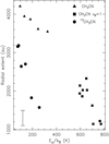 |
Fig. 6 ALMA 2019 data: plot of the radial extent of the velocity profile vs. the energy of the upper level of the transition for the molecular lines listed in Table 1. Triangles, squares, and circles refer to transitions of CH3CN, CH3CN v8 = 1, and 13CH3CN, respectively.The error bar in the lower left corner indicates the spatial resolution. |
4.2 Physical conditions in the molecular disk
We consider now the physical conditions of the gas in the molecular disk. In Sect. 3.2, we determined the rotational temperature,  K, and column density,
  , of 13CH3CN, which can be used to estimate the properties of the gas in the disk. Using the expression for the isotopic ratio 12C∕13C ≈ 7.5 × dgal + 7.6 (Wilson & Rood 1994), where dgal is the galactic distance, and the value of dgal = 3.6 kpc suitable for the G24.78+0.08 region, we derive 12C∕13C ≈ 35. Recent detailed ALMA studies of the CH3CN abundance (with respect to H2) in massive hot molecular cores indicate an average value of [CH3CN/H2] of ~ 10−9 (Pols et al. 2018). From the above values of 12C∕13C and [CH3CN/H2], and the 13CH3CN column density, we obtain an H2 column density of log10 [Ncol ∕ cm−2] ~ 26. Inspecting the PV plot of Fig. 4c, we deduce that the 13CH3CN emission is mainly found at radii between 500 au and 1000 au. Taking 1500 au as a crude estimate of the disk diameter, we calculate the H2 number density in the disk to be
  cm−3. At such a high density, the molecular rotational transitions should be mainly excited via collisions; therefore, the rotational temperature of 13CH3CN should be a reliable estimate of the gas kinetic temperature. The derived values of density,
  cm−3, and temperature,
  K, are consistent with the simulations from Tanaka et al. (2016), in which the molecular disk around a 20 M⊙ star, at radii ≲1000 au, has a gas (number) density of ~ 109 cm−3 (Tanaka et al. 2016, their Fig. 6, left panel) and a temperature between 100 K and 400 K (Tanaka et al. 2016, their Fig. 4).
Finally, we wanted to estimate the disk mass and the final mass of the YSO. Assuming that the disk is close to being edge-on, its projection on the sky falls inside a rectangle centered on the HC H II region and oriented at PA = 133°, with a major side of 8000 au (that is, two times the radial extension of the molecular velocity profiles in Fig. 4) and a minor side of 2000 au, which is large enough to include the whole HC H II region. Integrating the 1.4 mm continuum emission observed by Moscadelli et al. (2018) over this rectangle, we derive a flux of ≈120 mJy. After correcting for the dominant free-free contribution from the HC H II region of ≳86 mJy (Moscadelli et al. 2018, see their Sect. 5.1), the residual flux from dust emission is ≲ 120−86 = 34 mJy. Assuming, as Moscadelli et al. (2018) did, a dust opacity of 1 cm2 g−1 at 1.4 mm (Ossenkopf & Henning 1994), a gas-to-dust mass ratio of 100, and an average dust temperature over the disk of 200 K (in agreement with the aforementioned model by Tanaka et al. 2016), we derive an upper limit for the total mass of molecular gas in the disk of ≲2.5 M⊙. The mass of the ionized disk should be negligible with respect to this upper limit. We can estimate the radius of the ionized disk using the expression  for the radius of a gravitationally trapped H II region (where M⋆ is the stellar mass and cs is the sound speed in the ionized gas; Keto 2007, Eq. (3)). For cs = 13 km s−1 and M⋆ = 20 M⊙, we obtain Rb = 54 au. For such a small radius, the density in the ionized gas should be too high, nH ≥ 1012 cm−3, to yield a non-negligible mass for the ionized disk of ~ 1 M⊙. Therefore, we can conclude that the mass of the whole (molecular and ionized) disk is ≲10% of the mass, ≈20 M⊙, of the central star. This result is consistent with the Keplerian velocity profiles of the molecular tracers presented in Fig. 4.
In the scenario where the star is accreting only from its parental core, A1, the molecular mass inside core A1 of 4–7 M⊙ (evaluated by Moscadelli et al. 2018, see their Sect. 5.1) represents an upper limit for the stellar mass reservoir, such that the final mass of the star should be ≲30 M⊙. However, the final stellar mass could be larger than this value if the star gains its mass from the molecular clump enshrouding A1. The elongated (SE-NW) distribution of the cores (see Fig. 1) suggests that they are denser fragments from a more tenuous filamentary structure of molecular gas. It is therefore possible that the gravitational well of the star at the center of the HC H II region, being the most massive star in the cluster, induces mass inflows from the nearby cores.
5 Conclusions
We observed the HC (size ≈1000 au) H II region (ionized by a ZAMS star of ≈20 M⊙) inside molecular core A1 of the high-mass star-forming cluster G24.78+0.08 using ALMA at 1.4 mm during Cycle 6. By achieving an angular resolution of ≈0.′′050, corresponding to ≈330 au at the target distance of 6.7 kpc, we resolved the internal kinematics of the ionized gas and found, inside a region of radius ≲500 au, two mutually perpendicular VLSR gradients: one with a larger amplitude, 22 km s−1 mpc−1, directed along the axis at PA = 39°; the other with an amplitude of 3 km s−1 mpc−1 and orientedat PA = 133°. Along the axis at PA = 133°, the PV plots of different molecular tracers show similar velocity profiles that are consistent with Keplerian rotation around a 20 M⊙ star. We interpret these findings in terms of a disk that is molecular in the outer region, is internally ionized, and is in rotation around the massive star responsible for the H II region, plus a fast ionized jet collimated along the disk rotation axis (at PA = 39°).
To our knowledge, this is the first case in which both the ionized and molecular parts of a rotating disk have been detected, extending from inside to outside an HC H II region, over radii between 100 au and 4000 au. Toward the HC H II region in G24.78+0.08, the coexistence, from large to small scales, of mass infall (at a rate of ~ 10−3 M⊙ yr−1 at radii of ~5000 au; Beltrán et al. 2006), an outer molecular disk (from ≲4000 au to ≳500 au), and an inner ionized disk (≲500 au) ensures that the massive ionizing star is still actively accreting from its parental molecular core. These observations agree with recent models of massive star formation that include feedback of photoionization and radiation forces from the forming massive star (Tanaka et al. 2016; Kuiper & Hosokawa 2018) and support the view of a similar disk-mediated formation process for stars of all masses.
Acknowledgements
This paper makes use of the following ALMA data: ADS/JAO.ALMA#2018.1.00745.S. ALMA is a partnership of ESO (representing ts member states), NSF (USA) and NINS (Japan), together with NRC (Canada), MOST and ASIAA (Taiwan), and KASI (Republic of Korea), in cooperation with the Republic of Chile. The Joint ALMA Observatory is operated by ESO, AUI/NRAO and NAOJ. V.M.R. has received funding from the Comunidad de Madrid through the Atracción de Talento Investigador (Doctores con experiencia) Grant (COOL: Cosmic Origins Of Life; 2019-T1/TIC-15379).
References
- Anglada, G., Rodríguez, L. F., & Carrasco-González, C. 2018, A&ARv, 26, 3 [NASA ADS] [CrossRef] [Google Scholar]
- Beltrán, M. T., Cesaroni, R., Codella, C., et al. 2006, Nature, 443, 427 [NASA ADS] [CrossRef] [PubMed] [Google Scholar]
- Beltrán, M. T., Cesaroni, R., Moscadelli, L., & Codella, C. 2007, A&A, 471, L13 [NASA ADS] [CrossRef] [EDP Sciences] [Google Scholar]
- Beltrán, M. T., Cesaroni, R., Zhang, Q., et al. 2011, A&A, 532, A91 [CrossRef] [EDP Sciences] [Google Scholar]
- Briggs, D. S. 1995, BAAS, 27, 1444 [Google Scholar]
- Caratti o Garatti, A., Stecklum, B., Garcia Lopez, R., et al. 2017, Nat. Phys., 13, 276 [NASA ADS] [CrossRef] [Google Scholar]
- Cesaroni, R., Felli, M., Jenness, T., et al. 1999, A&A, 345, 949 [NASA ADS] [Google Scholar]
- Cesaroni, R., Beltrán, M. T., Moscadelli, L., Sánchez-Monge, Á., & Neri, R. 2019, A&A, 624, A100 [NASA ADS] [CrossRef] [EDP Sciences] [Google Scholar]
- De Pree, C. G., Wilner, D. J., Kristensen, L. E., et al. 2020, AJ, 160, 234 [Google Scholar]
- Franco-Hernández, R., & Rodríguez, L. F. 2004, ApJ, 604, L105 [NASA ADS] [CrossRef] [Google Scholar]
- Galván-Madrid, R., Rodríguez, L. F., Ho, P. T. P., & Keto, E. 2008, ApJ, 674, L33 [NASA ADS] [CrossRef] [Google Scholar]
- Hollenbach, D., Johnstone, D., Lizano, S., & Shu, F. 1994, ApJ, 428, 654 [NASA ADS] [CrossRef] [Google Scholar]
- Hosokawa, T., Yorke, H. W., & Omukai, K. 2010, ApJ, 721, 478 [NASA ADS] [CrossRef] [Google Scholar]
- Hunter, T. R., Brogan, C. L., MacLeod, G., et al. 2017, ApJ, 837, L29 [NASA ADS] [CrossRef] [Google Scholar]
- Jiménez-Serra, I., Báez-Rubio, A., Martín-Pintado, J., Zhang, Q., & Rivilla, V. M. 2020, ApJ, 897, L33 [Google Scholar]
- Keto, E. 2002, ApJ, 568, 754 [NASA ADS] [CrossRef] [Google Scholar]
- Keto, E. 2003, ApJ, 599, 1196 [NASA ADS] [CrossRef] [Google Scholar]
- Keto, E. 2007, ApJ, 666, 976 [NASA ADS] [CrossRef] [Google Scholar]
- Keto, E., & Klaassen, P. 2008, ApJ, 678, L109 [NASA ADS] [CrossRef] [Google Scholar]
- Klaassen, P. D., Johnston, K. G., Urquhart, J. S., et al. 2018, A&A, 611, A99 [NASA ADS] [CrossRef] [EDP Sciences] [Google Scholar]
- Kuiper, R., & Hosokawa, T. 2018, A&A, 616, A101 [NASA ADS] [CrossRef] [EDP Sciences] [Google Scholar]
- Kurtz, S. 2005, IAU Symp. 227, 111 [NASA ADS] [CrossRef] [Google Scholar]
- McMullin, J. P., Waters, B., Schiebel, D., Young, W., & Golap, K. 2007, ASP Conf. Ser., 376, 127 [Google Scholar]
- Meyer, D. M. A., Vorobyov, E. I., Kuiper, R., & Kley, W. 2017, MNRAS, 464, L90 [NASA ADS] [CrossRef] [Google Scholar]
- Möller, T., Endres, C., & Schilke, P. 2017, A&A, 598, A7 [NASA ADS] [CrossRef] [EDP Sciences] [Google Scholar]
- Moscadelli, L., Goddi, C., Cesaroni, R., Beltrán, M. T., & Furuya, R. S. 2007, A&A, 472, 867 [NASA ADS] [CrossRef] [EDP Sciences] [Google Scholar]
- Moscadelli, L., Sánchez-Monge, Á., Goddi, C., et al. 2016, A&A, 585, A71 [NASA ADS] [CrossRef] [EDP Sciences] [Google Scholar]
- Moscadelli, L., Rivilla, V. M., Cesaroni, R., et al. 2018, A&A, 616, A66 [NASA ADS] [CrossRef] [EDP Sciences] [Google Scholar]
- Moscadelli, L., Sanna, A., Cesaroni, R., et al. 2019, A&A, 622, A206 [NASA ADS] [CrossRef] [EDP Sciences] [Google Scholar]
- Ossenkopf, V.,& Henning, T. 1994, A&A, 291, 943 [Google Scholar]
- Peters, T., Banerjee, R., Klessen, R. S., et al. 2010a, ApJ, 711, 1017 [NASA ADS] [CrossRef] [Google Scholar]
- Peters, T., Mac Low, M.-M., Banerjee, R., Klessen, R. S., & Dullemond, C. P. 2010b, ApJ, 719, 831 [Google Scholar]
- Pols, S., Schwörer, A., Schilke, P., et al. 2018, A&A, 614, A123 [NASA ADS] [CrossRef] [EDP Sciences] [Google Scholar]
- Pudritz, R. E., Ouyed, R., Fendt, C., & Brandenburg, A. 2007, in Protostars and Planets V, eds. B. Reipurth, D. Jewitt, & K. Keil (Tucson: University of Arizona Press), 277 [Google Scholar]
- Purser,S. J. D., Lumsden, S. L., Hoare, M. G., et al. 2016, MNRAS, 460, 1039 [NASA ADS] [CrossRef] [Google Scholar]
- Purser, S. J. D., Lumsden, S. L., Hoare, M. G., & Kurtz, S. 2021, MNRAS, 504, 338 [CrossRef] [Google Scholar]
- Rivera-Soto, R., Galván-Madrid, R., Ginsburg, A., & Kurtz, S. 2020, ApJ, 899, 94 [CrossRef] [Google Scholar]
- Rodríguez, L. F., Gómez, Y., & Tafoya, D. 2007, ApJ, 663, 1083 [NASA ADS] [CrossRef] [Google Scholar]
- Rosero, V., Hofner, P., Claussen, M., et al. 2016, ApJS, 227, 25 [NASA ADS] [CrossRef] [Google Scholar]
- Rosero, V., Hofner, P., Kurtz, S., et al. 2019, ApJ, 880, 99 [NASA ADS] [CrossRef] [Google Scholar]
- Sanchez-Monge, A., Schilke, P., Ginsburg, A., Cesaroni, R., & Schmiedeke, A. 2018, A&A, 609, A101 [NASA ADS] [CrossRef] [EDP Sciences] [Google Scholar]
- Sanna, A., Moscadelli, L., Goddi, C., Krishnan, V., & Massi, F. 2018, A&A, 619, A107 [NASA ADS] [CrossRef] [EDP Sciences] [Google Scholar]
- Sanna, A., Moscadelli, L., Goddi, C., et al. 2019, A&A, 623, L3 [NASA ADS] [CrossRef] [EDP Sciences] [Google Scholar]
- Sewiło, M., Churchwell, E., Kurtz, S., Goss, W. M., & Hofner, P. 2008, ApJ, 681, 350 [NASA ADS] [CrossRef] [Google Scholar]
- Tan, J. C., Beltrán, M. T., Caselli, P., et al. 2014, Protostars and Planets VI (Tucson: University of Arizona Press), 149 [Google Scholar]
- Tanaka, K. E. I., Tan, J. C., & Zhang, Y. 2016, ApJ, 818, 52 [NASA ADS] [CrossRef] [Google Scholar]
- Tanaka, K. E. I., Zhang, Y., Hirota, T., et al. 2020, ApJ, 900, L2 [CrossRef] [Google Scholar]
- Wilson, T. L.,& Rood, R. 1994, ARA&A, 32, 191 [Google Scholar]
- Zhang, Q., Claus, B., Watson, L., & Moran, J. 2017, ApJ, 837, 53 [NASA ADS] [CrossRef] [Google Scholar]
- Zhang, Y., Tanaka, K. E. I., Rosero, V., et al. 2019, ApJ, 886, L4 [CrossRef] [Google Scholar]
The distance toward G24.78+0.08 has recently been determined via the trigonometric parallax measurement of the 6.7 GHz methanol masers (Moscadelli et al, in prep.).
All Tables
All Figures
|
Fig. 1 ALMA 2015 and JVLA observations of the high-mass star-forming region G24.78+0.08. The grayscale image shows the ALMA 1.4 mm continuum, with the intensity scale shown to the right of the panel. The black contour is the 7σ threshold of 1.2 mJy beam−1. The continuum emission fragments into distinct cores, labeled following Beltrán et al. (2011). The red contours reproduce the JVLA A-Array 1.3 cm continuum observed by Moscadelli et al. (2018), plotting levels from 0.3 to 16.3 in steps of 4 mJy beam−1. The insets in the lower left and right corners of the plot show the ALMA and JVLA beams, respectively. |
| In the text | |
|
Fig. 2 HC H II region. Upper panel: ALMA 2019 data: intensity-weighted velocity (color map) of the H30α emission, obtained from averaging the channel maps produced with a natural weighting of the uv -data. The beam (FWHM 0.′′080 × 0.′′062, with PA = 75°) is shown in the lower left corner. The black contours represent the velocity-integrated intensity of the H30α line, showinglevels from 0.26 to 1.3 in steps of 0.13 Jy beam−1 km s−1. The dashedblack rectangle delimits the field of view shown in the lower panel. Lower panel: ALMA 2015, VLA, and Very Long Baseline Interferometry (VLBI) data. The grayscale image represents the VLA A-Array 7 mm continuum observed by Beltrán et al. (2007). The white triangles and yellow squares mark the VLBI positions of the H2O 22 GHz (Moscadelli et al. 2007) and CH3OH 6.7 GHz masers (Moscadelli et al. 2018), respectively; the area of the symbol is proportional to the logarithm of the maser intensity. The white arrows show the proper motions of the H2O masers, which were first reported and analyzed in Moscadelli et al. (2007). The colored dots give the channel peak positions of the H30α line emissionobtained by Moscadelli et al. (2018) from ALMA data with 0.′′2 resolution; the colors denote the VLSR as indicated to the right of the plot. The dashed black line marks the axis of the spatial distribution of the H30α peaks. |
| In the text | |
|
Fig. 3 ALMA 2019 data. Upper panel: intensity-weighted velocity (color map) of the H30α emission, obtained from averaging the channel maps produced by weighting the uv -data with the “Briggs” robust parameter set to 0.5. The circular restoring beam has a FWHM size (0.′′ 058) equal to the geometric mean of the FWHM major and minor sizes of the Briggs beam and is shown in the lower left corner. The straight line indicates the direction, at PA = 133°, that connects the pixels of maximum and minimum velocity. The ALMA 1.4 mm continuum is represented with black contours, ranging from 3.2 to 10.6 in steps of 1.1 mJy beam−1. The beam of the continuum map is reported in the lower right corner. Lower panel: color map and white contours showing the PV plot of the H30α line along the cut at PA = 133°. The contour levels range from 4.9 to 24.6 in steps of 4.9 mJy beam−1. The vertical and horizontal white axes denote the positional offset (≈ −0.′′68) and VLSR (≈112 km s−1) of the YSO, respectively. In the lower right corner, the vertical and horizontal yellow error bars indicate the velocity and spatial resolutions, respectively. |
| In the text | |
|
Fig. 4 ALMA 2019 data. Each panel presents the combined PV plots, along the cut at PA = 133°, of the H30α emission (white contours; same as Fig. 3, lower panel) and a selected molecular line (color map): CH3CN JK = 123–113 (a); CH3CN JK = 126 –116 (b); 13CH3CN JK = 133–123 (c); and CH3CN v8 = 1 JK,l = 122,1–112,1 (d). Panels b and d: emission of other transitions close in frequency to the selected line. In each panel, the vertical and horizontal white axes denote the positional offset (≈ −0.′′68) and VLSR (≈112 km s−1) of the YSO, respectively. The magenta curve shows the Keplerian velocity profile for a central mass of 20 M⊙. In the lower left corner, the vertical and horizontal white error bars indicate the velocity and spatial resolutions, respectively. |
| In the text | |
|
Fig. 5 ALMA 2019 data: observed spectrum (black line) of SPW 6 across a frequency range covering the 13CH3CN JK = 13K–12K, K = 0–5, lines. The emission is averaged over a circle of 0.′′1 radius toward the center of the HC H II region. The fit (red histogram) of the 13CH3CN JK = 13K–12K, K = 0–5, lines performed with XCLASS is also reported. |
| In the text | |
|
Fig. 6 ALMA 2019 data: plot of the radial extent of the velocity profile vs. the energy of the upper level of the transition for the molecular lines listed in Table 1. Triangles, squares, and circles refer to transitions of CH3CN, CH3CN v8 = 1, and 13CH3CN, respectively.The error bar in the lower left corner indicates the spatial resolution. |
| In the text | |
Current usage metrics show cumulative count of Article Views (full-text article views including HTML views, PDF and ePub downloads, according to the available data) and Abstracts Views on Vision4Press platform.
Data correspond to usage on the plateform after 2015. The current usage metrics is available 48-96 hours after online publication and is updated daily on week days.
Initial download of the metrics may take a while.