| Issue |
A&A
Volume 650, June 2021
|
|
|---|---|---|
| Article Number | A168 | |
| Number of page(s) | 17 | |
| Section | Interstellar and circumstellar matter | |
| DOI | https://doi.org/10.1051/0004-6361/202039669 | |
| Published online | 23 June 2021 | |
Linking ice and gas in the λ Orionis Barnard 35A cloud
1
Niels Bohr Institute & Centre for Star and Planet Formation, University of Copenhagen,
Øster Voldgade 5−7,
1350
Copenhagen K., Denmark
e-mail: giulia.perotti@nbi.ku.dk
2
School of Physical Sciences, The Open University,
Walton Hall,
Milton Keynes,
MK7 6AA, UK
3
Department of Space, Earth, and Environment, Chalmers University of Technology, Onsala Space Observatory,
439 92
Onsala, Sweden
4
Space Telescope Science Institute,
3700 San Martin Drive,
Baltimore,
MD
21218, USA
Received:
13
October
2020
Accepted:
14
April
2021
Context. Dust grains play an important role in the synthesis of molecules in the interstellar medium, from the simplest species, such as H2, to complex organic molecules. How some of these solid-state molecules are converted into gas-phase species is still a matter of debate.
Aims. Our aim is to directly compare ice and gas abundances of methanol (CH3OH) and carbon monoxide (CO) obtained from near-infrared (2.5−5 μm) and millimetre (1.3 mm) observations and to investigate the relationship between ice, dust, and gas in low-mass protostellar envelopes.
Methods. We present Submillimeter Array (SMA) and Atacama Pathfinder EXperiment (APEX) observations of gas-phase CH3OH (JK = 5K−4K), 13CO, and C18O (J = 2−1) towards the multiple protostellar system IRAS 05417+0907, which is located in the B35A cloud, λ Orionis region. We use archival IRAM 30 m data and AKARI H2O, CO, and CH3OH ice observations towards the same target to compare ice and gas abundances and directly calculate CH3OH and CO gas-to-ice ratios.
Results. The CO isotopologue emissions are extended, whereas the CH3OH emission is compact and traces the giant molecular outflow emanating from IRAS 05417+0907. A discrepancy between sub-millimetre dust emission and H2O ice column density is found for B35A−4 and B35A−5, similar to what has previously been reported. B35A−2 and B35A−3 are located where the sub-millimetre dust emission peaks and show H2O column densities lower than that of B35A−4.
Conclusions. The difference between the sub-millimetre continuum emission and the infrared H2O ice observations suggests that the distributions of dust and H2O ice differ around the young stellar objects in this dense cloud. The reason for this may be that the four sources are located in different environments resolved by the interferometric observations: B35A−2, B35A−3, and, in particular, B35A−5 are situated in a shocked region that is plausibly affected by sputtering and heating, which in turn impacts the sub-millimetre dust emission pattern, while B35A−4 is situated in a more quiescent part of the cloud. Gas and ice maps are essential for connecting small-scale variations in the ice composition with the large-scale astrophysical phenomena probed by gas observations.
Key words: ISM: molecules / stars: protostars / astrochemistry / molecular processes / ISM: individual objects: Orion
© ESO 2021
1 Introduction
The interaction between dust, ice, and gas is ubiquitous in star-forming regions, and it is essential for the synthesis of interstellar molecules, the main ingredients for the origin of life on Earth. In recent decades, the number of detected molecules in the interstellar medium (ISM) increased considerably (McGuire 2018) and with it the awareness of an interplay between solid and gaseous molecules in star-forming regions (Herbst & van Dishoeck 2009; Boogert et al. 2015; Jørgensen et al. 2020; Öberg & Bergin 2021). Some of the questions that remain to be answered regard the link between the distribution of solids (dust, ices) and gaseous molecules in molecular clouds and what this tells us about the solid-gas intertwined chemistries (e.g. the thermal andnon-thermal desorption mechanisms that release solid-state molecules into the gas phase and vice versa).
Desorption mechanisms are of the utmost importance for understanding some critical aspects of star and planet formation (van Dishoeck & Blake 1998). Besides enhancing the chemical complexity in the gas phase (Cazaux et al. 2003; Jørgensen et al. 2016; Bergner et al. 2017; Calcutt et al. 2018; Manigand et al. 2020; van Gelder et al. 2020), the positions in protostellar disks at which they occur (i.e. snow lines) influence the formation and evolution of planets (Öberg et al. 2011; Eistrup et al. 2016; van ’t Hoff et al. 2017; Grassi et al. 2020). Simultaneously, desorption processes can also shape the composition of grain surfaces. This is a consequence of the fact that all desorption mechanisms are much more efficient for volatile species (CO, O2, and N2 ; Bisschop et al. 2006; Noble et al. 2012; Cazaux et al. 2017) than for less volatile species (H2O and CH3OH; Fraser et al. 2001; Bertin et al. 2016; Cruz-Diaz et al. 2016; Martín-Doménech et al. 2016). Since thermal desorption mechanisms alone can often not account for the diversity of species observed in star-forming regions, a further question remains as to the extent that the prevailing physical conditions might impact ice loss, for example through photo-desorption, sputtering, and chemical- and shock-induced processes (e.g. Kristensen et al. 2010; Vasyunin & Herbst 2013; Dulieu et al. 2013; Öberg 2016; Dartois et al. 2019). Obtaining key insights into the desorption mechanisms is crucial for studying the composition of ice mantles, and hence the production of complex organics, during the early phases of star formation.
The preferred observational approach for constraining solid-state chemistry consists of inferring abundances of solid-state molecules based on their observed gas-phase emissions (Bergin & Tafalla 2007; Öberg et al. 2009; Whittet et al. 2011). Although this method of indirectly deriving ice abundances from gas-phase observations is the most used to get insights into the ice composition, it relies on major assumptions, for instance on the formation pathways and the desorption efficiency of solid-state species.
One way to test these assumptions is to combine ice and gas observations (i.e. ice- and gas-mapping techniques) and thus compare ice abundances with gas abundances towards the same region (Noble et al. 2017; Perotti et al. 2020). The evident advantage of combining the two techniques is that it enables us to study the distribution of gas-phase and solid-state molecules concurrently on the same lines of sight, and hence to address how solid-state processes are affected by physical conditions probed by gas-phase mapping, such as density, temperature and radiation field gradients, turbulence, and dust heating. However, the number of regions where such combined maps are available is still limited.
In this article we explore the interplay between ice and gas in the bright-rimmed cloud Barnard 35 (B35A; also known as BRC18, SFO18, and L1594), which is located in the λ Orionis star-forming region (Sharpless 1959; Lada & Black 1976; Murdin & Penston 1977; Mathieu 2008; Hernández et al. 2009; Bayo et al. 2011; Barrado et al. 2011; Kounkel et al. 2018; Ansdell et al. 2020) at a distance of 410 ± 20 pc (Gaia DR2; Zucker et al. 2019, 2020). The λ Orionis region is characterised by a core of OB stars enclosed in a ring of dust and gas (Wade 1957; Heiles & Habing 1974; Maddalena & Morris 1987; Zhang et al. 1989; Lang et al. 2000; Dolan & Mathieu 2002; Sahan & Haffner 2016). The OB stars formed approximately 5 Myr ago, whereas the timing of the ring formation is less certain; it occurred between 1 and 6 Myr ago as the consequence of a supernova explosion (Dolan & Mathieu 1999, 2002; Kounkel 2020). The presence of strong stellar winds from the massive stars and ionisation fronts in the region has shaped and ionised the neighbouring ring of gas, leading to the formation of dense molecular clouds (e.g. B35A and B30; Barrado et al. 2018) and photodissociation regions (PDRs; Wolfire et al. 1989; De Vries et al. 2002; Lee et al. 2005). For instance, the stellar wind from λ Orionis, the most massive star of the Collinder 69 cluster (an O8III star; Conti & Leep 1974), hits the western side of B35A, compressing the cloud and forming a PDR between the molecular cloud edge and the extended HII region S264 (De Vries et al. 2002; Craigon 2015).
Star formation is currently occurring in B35A: the multiple protostellar system IRAS 05417+0907 (i.e. B35A−3) lies within the western side of the cloud (Fig. 1). IRAS 05417+0907 was long thought to be a single source, but it is in fact a cluster of at least four objects (B35A−2, B35A−3, B35A−4, and B35A−5), which were partially resolved by Spitzer InfraRed Array Camera (IRAC) observations as part of the Spitzer Legacy Program “From Molecular Cores to Planet-forming Disks1 ” (“c2d”; Evans et al. 2014; Table 1). B35A−3 (i.e. IRAS 05417+0907) is a Class I young stellar object (YSO), and it is the primary of a close binary system (Connelley et al. 2008); the classification of the other sources remains uncertain. B35A−3 emanates a giant bipolar molecular outflow extending in the NE-SW direction relative to λ Orionis and terminating at the Herbig-Haro object HH 175 (Myers et al. 1988; Qin & Wu 2003; Craigon 2015; Reipurth 2000). A detailed multi-wavelength analysis and characterisation of HH 175 and of the multiple protostellar system is presented by Reipurth & Friberg (2021).
The ice reservoir towards the YSOs in B35A has been extensively studied by Noble et al. (2013, 2017) and Suutarinen (2015). These works were based on near-infrared (NIR) spectroscopic observations (2.5−5 μm) with the AKARI satellite. In Noble et al. (2013), H2O, CO2, and CO ice features were identified towards all four YSOs; Suutarinen (2015) performed a multi-component, multi-line fitting of all the ice features towards the same B35A sources identified by Noble et al. (2013) and Evans et al. (2014) and, in a method similar to that employed by Perotti et al. (2020), were able to concurrently extract the H2O, CO, and CH3OH ice column densities from the spectral data. These are the ice column densities used for comparison in the remainder of this paper.
In parallel, the morphology and kinematics of the gas in B35A have been investigated using single dishes, such as the James Clerk Maxwell Telescope (JCMT) and the Institut de Radio Astronomie Millimétrique (IRAM) 30 m telescope by Craigon (2015). The survey mapped 12CO, 13 CO, and C18 O J = 3−2 and J = 2−1 over a 14.6′ × 14.6′ region and confirmed the existence of a bright and dense rim along the western side of B35A, which is heated and compressed by the stellar wind of the nearby λ Orionis, and of a giant bipolar outflow emanating from the YSO region.
To investigate the interaction between the solid (ice) and gas phases in the region, ice maps of B35A were compared to gas-phase maps in Noble et al. (2017). No clear correlation was found between gas or dust to ice towards B35A from this combination of ice- and gas-mapping techniques. The local scale variations traced by the ice mapping were not immediately related to large-scale astrophysical processes probed by the dust and gas observations.
In this paper, we present interferometric Submillimeter Array (SMA) observations of the JK = 5K−4K rotational band of CH3OH at 241.791 GHz and of the J = 2−1 rotational bands of two CO isotopologues (13CO and C18O) towards the multiple protostellar system IRAS 05417+0907 in B35A. The angular resolution of the interferometric observations allows us to study the distribution of the targeted species in greater spatial detail compared to existing single-dish observations. To also recover the large-scale emission, the SMA observations are combined with single-dish data, thus resolving the protostellar system members and, concurrently, probing the surrounding cloud. Furthermore, we produce ice and gas maps of a pivotal complex molecule, CH3OH, and of one of its precursors, CO, to analyse the gas and ice interplay in the region. Lastly, we directly calculate the gas-to-ice ratios of B35A to compare them with ratios obtained for nearby star-forming regions.
The article is organised as follows. Section 2 describes the gas-phase observations and the archival data used to produce the gas and ice maps. Section 3 presents the results of the observations. Section 4 analyses the variations between the gas-phase and solid-state distributions of the different molecules. Section 5 discusses the observational results with a particular focus on the obtained gas-to-ice ratios. Finally, Sect. 6 summarises the main conclusions.
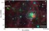 |
Fig. 1 Three-colour image of B35A overlaid with SCUBA−2 850 μm density flux in units of mJy beam−1 (Reipurth & Friberg 2021); contours are in decreasing steps of 30% starting at 7.3 Jy beam−1. The composite is made from Spitzer IRAC 3.6 μm (blue), 4.5 μm (green), and Multiband Imaging Photometer for Spitzer (MIPS) 24.0 μm (red) bands (programme ID: 139, PI: N. J. Evans II). The white stars mark the positions of the AKARI and Spitzer c2d identified B35A sources. Connelley et al. (2008) and Reipurth & Friberg (2021) show the B35A sources to be multiplet systems totalling four or five objects. |
Sample of sources.
2 Observations and archival data
2.1 SMA and APEX observations
The sample of sources was observed on September 19, 2018, with the SMA (Ho et al. 2004). The array was in its subcompact configuration with seven operating antennas. The targeted region was covered by two overlapping pointings; the first pointing was centred on B35A−3 (i.e. IRAS 05417+0907), and the second was offset by one half primary beam to the south-east. Their exact coordinates are αJ2000 = 05h44m30.s00, δJ2000 = +09° 08′ 57.′′ 3 and αJ2000 = 05h44m30.s58, δJ2000 = +09° 08′ 33.′′ 8, respectively.
The SMA observations probed frequencies spanning from 214.3 to 245.6 GHz with a spectral resolution of 0.1 MHz (0.135 km s−1). This frequency range covers, among other species, the CH3OH JK = 5K−4K branch at 241.791 GHz, 13CO J = 2−1 at 220.398 GHz, and C18O J = 2−1 at 219.560 GHz (Table 2). The observational setup consisted of a first long integration on the bandpass calibrator, the strong quasar 3c84, followed by alternated integrations on the source and on the gain calibrator, the quasar J0510+180. The absolute flux scale was obtained through observations of Uranus. The SMA dataset was both calibrated and imaged using the Common Astronomy Software Applications package2 (CASA; McMullin et al. 2007). At these frequencies, the typical SMA beam sizes were 7.′′ 3 × 2.′′4 with a position angle of −32.2° for CH3OH and 7.′′ 9 × 2.′′6 with a position angle of −31.2° for 13CO and C18O.
To trace the more extended structures in the region, the SMA data were complemented by maps obtained using the Atacama Pathfinder EXperiment (APEX; Güsten et al. 2006) on August 20−22, 2018. The single-dish observations covered frequencies between 236−243.8 GHz, matching the SMA 240 GHz receiver upper side band. The spectral resolution of the APEX observations was 0.061 MHz (0.076 km s−1). The APEX map size was 100″ × 125″, and it extended over both SMA primary beams. The coordinates of the APEX pointing are αJ2000 = 05h44m30. s00, δJ2000 = +09° 08′ 57.′′ 3. The APEX beam size was 27.′′4 for the CH3OH JK = 5K−4K lines emission. The APEX dataset was reduced using the GILDAS package CLASS3. At a later stage, the reduced APEX data cube was imported to CASA and combined with the interferometric data using the feathering technique. A description of the combination procedure is given in Appendix A.1.
2.2 JCMT/SCUBA-2, Spitzer IRAC, 2MASS, IRAM 30 m, and AKARI data
Ancillary data to the SMA and APEX observations were adopted in this study. To construct H2 column density maps of B35A, we used sub-millimetre continuum maps at 850 μm obtained with the SCUBA−2 camera at the JCMT by Reipurth & Friberg (2021), visual extinction values from the Spitzer c2d catalogue4, and 2MASSand Spitzer IRAC photometric data (Skrutskie et al. 2006; Evans et al. 2014). IRAM 30 m telescope observations (Craigon 2015) were used to trace the extended emission for 13CO and C18O J = 2−1. Finally, to produce gas-ice maps of B35A, we made use of the ice column densities determined by Suutarinen (2015) from AKARI satellite observations.
Spectral data of the detected molecular transitions.
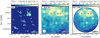 |
Fig. 2 Integrated intensity maps for 13CO J = 2−1 detected by the SMA (panel a), by the IRAM 30 m telescope (panel b), and in the combined interferometric SMA and single-dish IRAM 30 m data (panel c). All lines are integrated between 7 and 16 km s−1. Contours are at 5σ, 10σ, 15σ, etc. (σSMA = 0.42 Jy beam−1 km s−1, σIRAM 30 m = 6 Jy beam−1 km s−1, σSMA+IRAM 30 m = 1.03 Jy beam−1 km s−1). Panel c: white area outlines the primary beam of the SMA observations. The synthesised beams are displayed in white in the bottom left corner of each panel. The white stars mark the positions of the targeted B35A sources. |
3 Results
This sectionlists the observational results, supplying a summary of the methods employed to determine CO and CH3OH gas column densities (Sect. 3.1 and Appendix A). Additionally, it presents the H2O, CO, and CH3OH ice column densities (Sect. 3.2) and the two H2 column density maps used in the calculation of the abundances of the ice and gas species (Sect. 3.3).
3.1 Gas-phase species
The spectralline data of the detected molecular transitions are listed in Table 2. Figures 2–4 display moment 0 maps of the 13CO and C18O J = 2−1 lines and the CH3OH J = 50−40 A+ line createdusing SMA, IRAM 30 m, and APEX data. Moment 0 maps of the CH3OH J = 50−40 A+ line are presented in this section as this transition is the brightest of the CH3OH J = 5K−4K branch at 241.791 GHz. The maps show that the SMA observations filter out spatially extended emission related to the B35A cloud. The SMA data only recover ≈10% of the extended emission detected in the single-dish data. Consequently, we need to combine the interferometric data with the single-dish maps in order not to severely underestimate the column densities.
Panels a of Figs. 2–3 show that the interferometric emission is predominantly compact and the peak intensity is seen, for both CO isotopologues, at the location of B35A−2. The emission observed in the IRAM 30 m datasets (panels b of Figs. 2–3) is extended and mostly concentrated around B35A−2, B35A−3, and B35A−5. In the combined SMA + IRAM 30 m maps (panels c of Fig. 2–3), the peak emission is also located in the region where B35A−2, B35A−3, and B35A−5 are present.
In contrast, the observed CH3OH peak intensity is exclusively localised at the B35A−5 position in the SMA data (panel a of Fig. 4). B35A−5 lies along the eastern lobe of the giant bipolar molecular outflow emanated from IRAS 05417+0907 (i.e. B35A−3) and terminating at the location of the Herbig-Haro object HH 175 (Craigon 2015). The CH3OH emission is extended in the APEX data (panel b of Fig. 4) and hence not resolved at one particular source position. The emission in the SMA + APEX moment 0 map (panel c of Fig. 4) is compact and concentrated in one ridge in the proximity of B35A−5. The channel maps (Figs. A.3−A.5) and the spectra (Fig. A.1) extracted from the combined interferometric and single-dish datasets show predominantly blue-shifted components (Appendix A.3). Blue- and red-shifted components are seen for the CO isotopologues, which were previously observed by De Vries et al. (2002), Craigon (2015), and Reipurth & Friberg (2021) and attributed to outflowing gas.
The 13CO emission is optically thick towards the B35A sources; therefore, the 13CO column densities are underestimated towards the targeted region (Appendix A.2). Consequently, the optically thin C18 O emission was adopted to estimate the column density of 12CO in B35A. First, C18O column densities towards the protostellar system members were obtained from the integrated line intensities of the combined SMA + IRAM 30 m maps (panel c of Fig. 3), assuming optically thin emission and a kinetic temperature for the YSO region equal to 25 K (Craigon 2015). The formalism adopted in the column density calculation is presented in Appendix A.4, and the calculated C18 O column densities and their uncertainties are listed in Table 3. The C18 O column densities were converted to 12CO column densities, assuming a 16O/18O isotope ratioof 557 ± 30 (Wilson 1999). The resulting 12CO column densities (Table 3) are in good agreement with the values reported in Craigon (2015).
The CH3OH column density towards B35A−5 was estimated from the integrated line intensities of the combined SMA + APEX maps for the five CH3OH lines (Table A.2), assuming optically thin CH3OH emission, a kinetic temperature of 25 K (Craigon 2015), and local thermodynamic equilibrium (LTE) conditions. The CH3OH column density and its uncertainty are reported in Table 3. For all the gas-phase species, the uncertainty on the column densities was estimated based on the spectral rms noise and on the ~20% calibration uncertainty.
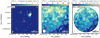 |
Fig. 3 Integrated intensity maps for C18O J = 2 detected by the SMA (panel a), by the IRAM 30 m telescope (panel b), and in the combined interferometric SMA and single-dish IRAM 30 m data (panel c). All lines are integrated between 10 and 15 km s−1. Contours are at 5, 10, and 15σ (σSMA = 0.37 Jy beam−1 km s−1, σIRAM 30 m = 5 Jy beam−1 km s−1, σSMA+IRAM 30 m = 0.40 Jy beam−1 km s−1). Panel c: white area outlines the primary beam of the SMA observations. The synthesised beams are displayed in white in the bottom left corner of each panel. The white stars mark the positions of the targeted B35A sources. |
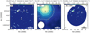 |
Fig. 4 Integrated intensity maps for CH3OH J = 50–40 A+ detected by the SMA (panel a), by the APEX telescope (panel b), and in the combined interferometric SMA and single-dish APEX data (panel c). All lines are integrated between 6 and 12.5 km s−1. Contours start at 5σ (σSMA = 0.04 Jy beam−1 km s−1, σAPEX = 4 Jy beam−1 km s−1, σSMA+APEX = 0.04 Jy beam−1 km s−1) and follow insteps of 5σ. Panel c: white area outlines the primary beam of the SMA observations. The synthesised beams are displayed in white in the bottom left corner of each panel. The white stars mark the positions of the targeted B35A sources, and the dotted blue line indicates the direction of the giant outflow terminating at HH 175. |
Total ice and gas column densities towards the B35A sources.
3.2 Ice column densities
The ice column densities of H2O, CO and CH3OH used in this paper were originally derived by Suutarinen (2015) from the AKARI (2.5−5 μm) NIR spectra of the targeted B35A sources. Suutarinen (2015) adopted a non-heuristic approach, employing ice laboratory data and analytical functions to concurrently account for the contribution of a number of molecules to the observed ice band features. A detailed description of the AKARI observations is given in Noble et al. (2013), and the methodology adopted to derive the column densities of the major ice species can be found in Suutarinen (2015).
The total ice column densities from Suutarinen (2015) are listed in Table 3. Among the three molecules, H2O ice is the most abundant in the ices of B35A, with column densities of up to 3.35 × 1018 cm−2, followed by CO and CH3OH (Table 3). The column densities of the latter two molecules are comparatively one order of magnitude less abundant than H2O ice. Upper limits are given for the CO and CH3OH column densities towards B35A−5 because of difficulties in distinguishing the absorption features in the spectrum of this YSO (Noble et al. 2013; Suutarinen 2015). A trend is observed for the CO and CH3OH values: The column densities towards B35A−2 are the highest reported, followed by B35A−3, B35A−4, and B35A−5. The CO and CH3OH ice column densities appear to follow the visual extinction, with B35A−2 and B35A−3 being the most extincted sources and showing the highest CO and CH3OH column densities (Tables 1 and 3). In this regard, it is important to recall that B35A−2 is not detectedin the J, H, or K bands, making the determination of its visual extinction uncertain (Sect. 3.3 and Appendix B).
3.3 H2 column densities
An important factor to consider when combining ice- and gas-mapping techniques is that ice absorption and dust and gas emissions may probe different spatial scales (Noble et al. 2017). As a matter of fact, the targeted sources may be embedded to different depths in the B35A cloud, and, consequently, the gas and ice observations may not be tracing the same columns of material. Therefore, the search for gas-ice correlations towards B35A has to be performed by comparing gas and ice abundances relative to H2, following the approach adopted in Perotti et al. (2020).
To keep the gas and ice observations in their own reference frame, two H2 column density maps were produced: one to derive gas abundances and one to determine ice abundances (Fig. 5). For the gas observations, estimates of the H2 column density were made using sub-millimetre continuum maps of B35A at 850 μm (SCUBA−2; Reipurth & Friberg 2021), under the assumption that the continuum emission originated from optically thin thermal dust radiation (Kauffmann et al. 2008). In this regime, the strength of the sub-millimetre radiation is dependent on the column density (N), the opacity (κν), and the dust temperature (T). The adopted value for the opacity per unit dust+gas mass at 850 μm was 0.0182 cm2 g−1 (‘OH5 dust’; Ossenkopf & Henning 1994). The temperature of B35A has been estimated by Morgan et al. (2008) and Craigon (2015). Both studies found two distinct regimes within the cloud: a cold region (Tgas = 10−20 K, Tdust = 18 K) in the shielded cloud interior located to the east of the YSOs and a warm region (Tgas = 20−30K) to the west of the YSOs. Since the region where the YSOs are located lies close to the western edge of the warm cloud, a Tdust = 25 K was adopted to estimate the H2 column density map illustrated in Fig. 5a based on Craigon (2015) and Reipurth & Friberg (2021). The H2 column density towards the B35A sources is reported in Table 3. The error on the H2 column density was estimated according to the 5% flux calibration uncertainty (Dempsey et al. 2013). It does not include the errors on Tdust due to the uncertainties on the upper and lower limits for Tdust in the YSO region.
Increasing the dust temperature to 30 K would lower the H2 column density by 22% and consequently increase the abundance of the gas-phase species by the same amount; on the other hand, lowering the dust temperature to 18 K would increase the H2 column density by 61% and consequently lower the gas abundance likewise. The above estimates assume an excitation temperature equal to 25 K for CO and CH3OH. Increasing both the excitation temperature and the dust temperature to 30 K would result in gas abundances increasing by 24%. Conversely, lowering both temperatures to 18 K would lower the abundances by 33%. A comprehensive description of the production of the H2 column density map from SCUBA−2 measurements is given in Appendix C of Perotti et al. (2020).
The H2 column density map calculated from the SCUBA−2 measurements supplies an accurate estimate of the total beam-averaged amount of gas towards B35A, and therefore provides a useful reference for the optically thin gas-phase tracers. However, the derived H2 column density map cannot be directly related to the AKARI data that supply (pencil-beam) measurements of the column densities towards the infrared sources that may or may not be embedded within the B35A cloud.
For the ice observations, the H2 column density map was therefore obtained by performing a linear interpolation of the tabulated visual extinction (AV) values for B35A taken from the Spitzer c2d catalogue5 (see Appendix B). Since no calculated AV values are reported for B35A−2 or B35A−3, the AV for B35A−3 was acquired by de-reddening the spectral energy distribution (SED) at the 2MASS J, H, and K photometric points to fit a blackbody and using a second blackbody to model the infrared excess at longer wavelengths. A detailed description of the fitting procedure adopted for B35A−3 is given in Appendix B. Following Evans et al. (2009) and Chapman et al. (2009), we adopted an extinction law for dense ISM gas with RV = 5.5 from Weingartner & Draine (2001) to calculate AV. The visual extinction for B35A−2 could not beestimated through a similar procedure due to the lack of NIR photometry data available for this object, and thus the AV for this source was obtained through the interpolation of the available visual extinction measurements for B35A. The final AV values of the four sources are listed in Table 1. Finally, the visual extinction was converted to H2 column density using the relation  cm−2 (AV/mag), which was established for dense ISM gas (Evans et al. 2009). The H2 column density calculated from the AV map is shown in Fig. 5b.
The H2 column densities calculated from both methods are of the same order of magnitude, 1022 cm−2 (Table 3). The column densities differ by approximately a factor of four, possibly due to variations in the exact column densities traced by SCUBA−2 and AV measurements as well as assumptions on the dust temperature. In both H2 column density maps (Figs. 5a,b), it is seen that the four sources lie in the densest region of the cloud, confirming the results previously presented in Craigon (2015) and Reipurth & Friberg (2021). Although the two maps were calculated using two different methods, they reproduce the same trend: B35A−2 and B35A−3 are located where the H2 column density peaks, whereas B35A−4 and B35A−5 are situated in less dense regions. However, in the H2 column density map calculated from the visual extinction (Fig. 5b), lower  values are reported for B35A−5 with respect to the other YSOs, whereas this is not the case in the H2 column density map calculated from the SCUBA−2 map (Fig. 5a), where lower
  values are observed for B35A−4. This difference can be explained by recalling that B35A−5 is the less extincted YSO (AV = 19.5 mag) and is located along the trajectory of the giant outflow launched by B35A−3. Consequently, the SCUBA−2 observations (14.6′′ beam) are likely tracing the more extended structure of the dust emission in the region and not resolving the more compact emission towards each individual object. It is worth recalling that embedded protostars and Herbig-Haro objects can substantially affect the dust emission morphology (Chandler & Carlstrom 1996); hence, the
  enhancement seen in Fig. 5a likely reflects dust heating by the embedded protostars and by HH175, resulting in an increase in the sub-millimetre continuum flux rather than in a higher column density.
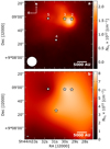 |
Fig. 5 H2 column density maps of B35A. a:
|


4 Analysis
4.1 Gas-ice maps
In Fig. 6 the distributions of gas-phase 13CO 2−1 (panel a) and C18O 2−1 (panel b) emissions are compared to CO ice abundances. Both CO isotopologue emissions are concentrated at the B35A−2, B35A−3, and B35A−5 source positions. The emission towards these three sources is of comparable intensity but drops in the surroundings of B35A−4, especially towards the southern edge of the cloud. The CO ice abundances with respect to H2 are not characterised by large variations; instead, they are quite uniform and consistent within the uncertainties (Table 4). Only an upper limit could be determined for the CO ice column density towards B35A−5 due to the uncertainty in distinguishing the absorption feature at 3.53 μm in the spectrum of this object.
In Fig. 6c the distribution of gas-phase CH3OH 50 −40 A+ emission is compared to CH3OH ice abundances. As described in Sect. 3.1, the CH3OH emission is concentrated solely in one ridge, located in the proximity of the B35A−5 position. At this location, only an upper limit on the CH3OH ice abundance could be determined. The morphology of the CH3OH emission suggests that while B35A−5 is situated in a shocked region, sitting along the trajectory of the giant outflow, B35A−4 lies in a more quiescent area that is less influenced by high-velocity flows of matter. The CH3OH ice abundances with respectto H2 are characterised by slightly larger variations compared to CO ice (Table 4).
Finally, in Fig. 6d, the distribution of gas-phase CH3OH 50 −40 A+ emission is compared toH2O ice abundances.The H2O ice abundances are approximately one order of magnitude higher than the CO and CH3OH ice abundances (Table 4). The lowest H2O ice abundance is reported towards B35A−5, where the CH3OH peak emission is observed. In contrast, the highest H2O ice abundance is obtained towards B35A−4, where CH3OH emission is not detected.
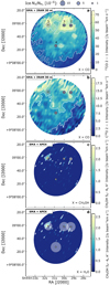 |
Fig. 6 Gas-ice maps of B35A. Ice abundances are indicated as filled grey (panels a and b) or white circles (panels c and d), and upper limits are displayed as empty circles. Contour levels are 5, 10, and 15σ. a: CO ice abundances on gas 13CO 2−1. b: CO ice abundances on gas C18O 2−1. c: CH3OH ice abundances on gas CH3OH 50−40 A+. d: H2O ice abundances on gas CH3OH 50−40 A+. The white area outlines the primary beam of the SMA observations. The white stars mark the positions of the targeted B35A sources. |
4.2 Gas and ice variations
In Fig. 7 the search for gas-ice correlations towards B35A is addressed by analysing gas and ice abundances relative to H2 (Table 4). The y-axes of all three panels display CO gas abundances, which are compared to abundances of CO ice (panel a), CH3OH ice (panel b), and H2O ice (panel c). To maintain gas and ice observations in their own reference frame, the CO gas abundances were estimated using  values calculated from SCUBA−2 850 μm maps, whereas the ice abundances were calculated using
  values obtained from the visual extinction map (see Sect. 3.3 and Appendix B). The formalism adopted to propagate the uncertainty from the column densities to the abundances is reported in Appendix A.4.
It is immediately apparent that none of the ice species exhibit a predictable trend in ice abundance with gas abundance. Panels a and b show a similar behaviour since they are comparing molecules that are chemically linked: CO gas versus CO ice and CO gas versus CH3OH ice, with CO being the precursor of CH3OH. At the same time, panel c does not display the same relationships seen in the previous two panels. The latter observation is not surprising since there is no reason for CO and H2O to be directly linked from a purely chemical perspective.
In both panels of Fig. 7, B35A−4 displays the highest CO gas and the lowest CO and CH3OH ice abundances. When the uncertainties are taken into account, the CO ice abundances towards B35A−2, B35A−3, and B35A−4 are alike (Table 4). For the CH3OH ice abundances,B35A−3 and B35A−4 are consistent within the error bars; only towards B35A−2 is a significant difference found. Both CO and CH3OH ice abundances towards B35A−5 are upper limits (Table 4). The similarity between CO and CH3OH ice trends and the fact that the CH3OH/CO ice ratios are >0.3 indicate an efficient CH3OH formation through CO hydrogenation (Watanabe & Kouchi 2002) on the grain surfaces of B35A. The CO gas abundances towards B35A−2, B35A−3, and B35A−5 are in agreement within the uncertainties (Table 4).
In panel c some of the gas-ice variations differ with respect to panels a and b: B35A−4 is characterised by the highest H2O ice abundance, whereas B35A−5 shows the lowest H2O ice abundance. This result corroborates the prediction that the ices of B35A−5 are the most depleted of volatile molecules among the B35A sources. The behaviours of B35A−2 and B35A−3 are similar if the uncertainties are considered (Table 4). The observed ice and gas variations between CO gas, CH3OH gas, and H2O ice towards B35A−4 and B35A−5 favour a scenario in which H2O ice is formed and predominantly resides on the ices of B35A−4, likely located in the most ‘quiescent’ area of the targeted region, whereas in the proximity of a shocked region (B35A−5), H2O ice mantles are partially desorbed. This result is discussed further in Sect. 5.1. Although the gas and ice variations analysed in this section and in Sect. 4.1 are based on a small sample, they still highlight interesting trends in accordance to what we would expect from our knowledge of the physical structure of the targeted region.
Iceand gas abundances relative to H2 towards the B35A sources.
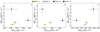 |
Fig. 7 Gas and ice variations in B35A. The circles represent the targeted B35A sources. Panels a–c: relation between CO, CH3OH, and H2O ice and CO gas abundances relative to H2. |
4.3 Comparison with previous gas-ice maps of B35A
Noble et al. (2017) produced the first gas-ice maps of B35A. They compared AKARI ice abundances from Noble et al. (2013) with: single-dish (JCMT/HARP and IRAM 30 m/HERA) gas-phase maps of C18O (Buckle et al. 2009; Craigon 2015; J = 3−2 and 2−1), sub-millimetre continuum SCUBA maps at 850 μm and 450 μm/850 μm (Di Francesco et al. 2008), and Herschel/SPIRE maps at 250 μm (Griffin et al. 2010). The H2 gas-phase map adopted to calculate ice abundances was determined from CO observations (Craigon 2015).
Noble et al. (2013, 2017) derived their ice column densities without considering the presence of CH3OH, and thus the H2O ice column densities were routinely higher than those used here from Suutarinen (2015; our Fig. 8). Simultaneously, the CO ice column densities were calculated using different laboratory data; for example, the CO-ice red component was fitted using a CO:H2O (Fraser & van Dishoeck 2004) laboratory spectrum as opposite to the CO:CH3OH mixture (Cuppen et al. 2011), resulting in a higher CO-ice column density compared to Suutarinen (2015).
The combination of gas, dust, and ice observations proposed in Noble et al. (2017) is characterised by a number of limitations that are taken into account in the presented work, including: the lower angular resolution of the adopted single-dish observations, the analysis of the chemical behaviours of only simple molecules (e.g. H2O, CO, and CO2), and not taking into account the fact that the ice and gas observations might probe different depths. The presented work overcomes these limitations by making use of higher angular resolution interferometric observations, studying the ice and gas variations of both simple (H2O, CO) and complex molecules (CH3OH), and, lastly, by comparing ice and gas abundances derived using two different H2 column density maps (to keep the ice and gas observations in their own reference frame).
From the analysis of the gas-ice maps, Noble et al. (2017) inferred that the dust in B35A is mainly localised around B35A−2 and B35A−3, in agreement with the higher ice column densities of H2O and CO towards these two sources (Fig. 8). However, they observed that the H2O ice column densities are lower towards B35A−5 compared to B35A−4, even though the dust emission is higher towards B35A−5. The authorsconclude that no clear trend between ice, dust, and gas is seen in B35A and that more knowledge of the local-scale astrophysical environment is needed to disentangle the exact interplay between ice and gas in the region. The findings of Noble et al. (2017) are in agreement with the observational results and the gas-ice maps of B35A presented here (with the caveat that both CO ice abundances towards B35A−5 in Noble et al. 2017 and in this work are upper limits). However, the gas-ice maps produced in this study show that the lower H2O ice abundance towards B35A−5 compared to B35A−4 is plausibly caused by the influence of shocks on the ice chemistry. CH3OH is a tracer of energetic inputs in the form of outflows (Kristensen et al. 2010; Suutarinen et al. 2014), and it traces the trajectory of the bipolar outflow in B35A. As a result, lower H2O ice abundances towards B35A−5 are likely the result of sputtering effects in the outflow shocks (e.g. Suutarinen et al. 2014 and references therein). Simultaneously, the fact that the sub-millimetre dust emission towards B35A−5 is high where the H2O ice abundances are lower can also be explained by the presence of the outflow terminating at the Herbig-Haro object HH 175. In fact, UV radiation generated in the Herbig-Haro object itself may locally heat the dust, enhancing the sub-millimetre continuum flux of the region (Chandler & Carlstrom 1996; Kristensen et al. 2010; Fig. 5a).
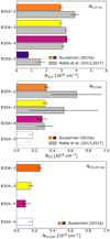 |
Fig. 8 H2O (top), CO (middle), and CH3OH (bottom) total ice column densities obtained in Suutarinen (2015, the sources are colour-coded) compared to Noble et al. (2017, light grey). The empty bars represent upper limits on the column densities. |
5 Discussion
The CH3OH gas abundances in B35A (10−8) are greater than what could be inferred by pure gas-phase synthesis (e.g. Garrod et al. 2006). Hence, the observed CH3OH gas must be produced on the grain surfaces and be desorbed afterwards. In the following, the preferred scenario for CH3OH desorption in B35A is discussed. Additionally, the observational results presented in Sects. 3.1−3.2 are employed to determine CH3OH and CO gas-to-ice ratios (Ngas/Nice) towards the multiple protostellar system in B35A. Finally, a comparison between the gas-to-ice ratios directly determined towards B35A and the gas-to-ice ratios of nearby star-forming regions is proposed.
5.1 Sputtering of CH3OH in B35A
Sections 3.1 and 4.1 showed that the CH3OH emission is concentrated almost exclusively in one ridge, which coincides with the B35A−5 position. B35A−5 sits along the eastern lobe of a large collimated outflow emanated from the binary Class I IRAS 05417+0907 (i.e. B35A − 3). The eastern lobe has a total extent of 0.6 pc, and it terminates at the Herbig-Haro object HH 175 (Craigon 2015). The total extent of the outflow is 1.65 pc (Reipurth & Friberg 2021), which places HH 175 among the several dozen Herbig-Haroobjects with parsec dimensions (Reipurth & Bally 2001). Herbig-Haro objects are omnipresent in star-formingregions, but it is still not clear how exactly they are tied into the global star-formation process, for example how they alter the morphology and kinematics of the gas in which they originate. These are highly energetic phenomena that are believed to form when high-velocity protostellar jets collide with the surrounding molecular cloud, inducing shocks. Such shocks compress and heat the gas, generating UV radiation (Neufeld & Dalgarno 1989). The activity of Herbig-Haro objects can dramatically change the chemical composition of the gas in their vicinity, mutating the chemistry of the region during so-called sputtering processes (Neufeld & Dalgarno 1989; Hollenbach & McKee 1989).
Sputtering takes place in shocks when neutral species (e.g. H2, H, or He) collide with the surface of ice-covered dust grains with sufficient kinetic energy to expel ice species (e.g. CH3OH, NH3, or H2O) into the gas phase (Jørgensen et al. 2004; Jiménez-Serra et al. 2008; Kristensen et al. 2010; Suutarinen et al. 2014; Allen et al. 2020). During a sputtering event, the ice molecules can desorb intact or be destroyed (e.g. via dissociative desorption) either due to the high kinetic energy or by reactions with H atoms (Blanksby & Ellison 2003; Dartois et al. 2019, 2020). The fragments of dissociated molecules can then readily recombine in the gas phase (Suutarinen et al. 2014 and references therein).
The inferred dust temperatures in the B35A region (20−30 K) are remarkably lower than the CH3OH sublimation temperature (~128 K; Penteado et al. 2017), which rules out thermal desorption as a potential mechanism triggering the observed CH3OH emission. This consideration, together with the observation of the CH3OH emission along the HH 175 flow direction and the anti-correlation between CH3OH emission and the lower H2O ice abundances towards B35A−5, suggests that ice sputtering in shock waves is a viable mechanism to desorb ice molecules in B35A. Simultaneously, the absence of shocks towards B35A−4 likely explains the highest abundance of H2O ice observedin this more quiescent region (Fig. 6d). Higher angular resolution observations of CH3OH in the region are required to provide quantitative measurements of the amount of CH3OH desorbed via sputtering compared to other non-thermal desorption mechanisms. Additional gas-phase observations of H2O towards the B35A sources are needed to further constrain the processes linking H2O ice and H2O gas in this shocked region (e.g. sputtering of H2O ice mantles versus direct H2O gas-phase synthesis) and, in a broader context, to help explain the high abundances of H2O observed in molecular outflows (Nisini et al. 2010; Bjerkeli et al. 2012, 2016; Santangelo et al. 2012; Vasta et al. 2012; Dionatos et al. 2013).
 |
Fig. 9 CH3OH (panel a) and CO (panel b) gas-to-ice ratios (Ngas/Nice) for the multiple protostellar system in Orion B35A and Serpens SVS 4. The dark green squares indicate the gas-to-ice ratios estimated by Perotti et al. (2020) for the Serpens SVS 4 cluster. The light green circles mark the ratios calculated in this study. The dotted light blue line in panel a represents the ratio estimated by Öberg et al. (2009) towards Class 0/I objects. The shaded areas indicate the estimated ranges of the gas-to-ice ratios. |
5.2 Gas-to-ice ratios
Figure 9 displays the CH3OH (panel a) and CO (panel b) gas-to-ice ratios towards ten sources constituting the SVS 4 cluster located in the Serpens molecular cloud (Perotti et al. 2020) and towards the B35A sources in the Orion molecular cloud. The shaded areas indicate the estimated ranges of gas-to-ice ratios towards both molecular clouds, providing complementary information about the gas-to-ice ratios of both regions compared to the value calculated towards each individual source.
Figure 9a shows the CH3OH gas-to-ice ratios ( /
/ ) towards the SVS 4 sources and B35A−5. Only an upper limit for the CH3OH gas-to-ice towards B35A−5 is obtained (i.e. 1.1 × 10⁻³) due to the uncertainty on the CH3OH ice column density determination towards this source (Suutarinen 2015). Therefore, only limited information is available regarding the CH3OH chemistry in B35A. Figure 9a also displays the averaged CH3OH gas-to-ice ratio towards four low-mass embedded protostars located in nearby star-forming regions from Öberg et al. (2009). A detailed comparison between the CH3OH gas-to-ice ratios for the SVS 4 cluster members and the value estimated by Öberg et al. (2009) is given in Perotti et al. (2020) and therefore not repeated here.
The observations of B35A address cold quiescent CH3OH emission (J = 5K −4K transitions at 241.7 GHz and Eu from 34.8 to60.7 K; see Table 2) and presumably quiescent gas not affected by outflow shocks and/or thermally desorbed in the vicinity of the protostar. The same applies to the observations presented in Öberg et al. (2009; J = 2−1 transitions at 96.7 GHz and Eu in the range 14.4−35.4 K). However, B35A−5 and the SVS 4 sources that report the highest gas-to-ice ratios are likely affected to some extent by outflow shocks (i.e. B35A−5 by the giant outflow terminating at HH 175 and the SVS 4 sources by the outflow known to be associated with SMM 4). This might justify the mismatch between the Öberg et al. (2009) value and the higher values of the gas-to-ice ratios. In the case of the B35A cloud, high-sensitivity infrared observations of B35A are required to further constrain this observation.
CO gas-to-ice ratios ( /
/ ) towards the SVS 4 and B35A sources are illustrated in Fig. 9b. As discussed previously in Perotti et al. (2020), the range of gas-to-ice ratios for SVS 4 extends between one and six, and it is significantly higher than the predicted value (~4 × 10⁻²; Cazaux et al. 2016). This theoretical prediction is estimated from the three-phase astrochemical model by Cazaux et al. (2016), which includes thermal and non-thermal desorption processes of the species constituting the ice mantles. This comparison with the theoretical prediction has to be taken with care since the physical model is not specifically tuned to reproduce the structures of the SVS 4 cluster or the B35A cloud. The estimated dust temperature towards the SVS 4 cluster is below 20 K (Kristensen et al. 2010), indicating that CO is likely frozen out on the grain surfaces. We concluded from the high relative CO gas abundances that the gas-mapping does not trace the densest regions of the SVS 4 cluster but rather an extended component that is not sensitive to the effects of freeze-out (Fig. 8 of Perotti et al. 2020).
High CO gas-to-ice ratios are also observed for B35A, but in this case they are mainly attributable to CO that is thermally desorbed in the region. The physical conditions of B35A and SVS 4 differ significantly; for example, the western side of B35A is highly influenced by the ionisation-shock front driven by the λ Orionis OB stars, and the dust temperature in the YSO region of B35A has been estimated to be at least 25−30 K (Craigon 2015; Morgan et al. 2008). Therefore, at these temperatures, which are above the CO sublimation temperature (~20 K; Bisschop et al. 2006; Collings et al. 2004; Acharyya et al. 2007), CO is efficiently thermally desorbed from the grain surfaces and is expected to primarily reside in the gas phase. According to this result, the observed CH3OH ice might have formed at earlier stages, prior to the warming of the dust grains, or, alternatively, from CO molecules trapped in porous H2O matrices, and is therefore not sublimated at these temperatures. Additionally, higher abundances of CO might reflect an active CO gas-phase synthesis in the region. Follow-up observations of higher J transitions of CO isotopologues are required to provide a conclusive assessment.
6 Conclusions
Millimetric (SMA, APEX, IRAM 30 m) and infrared (AKARI) observations were used to investigate the relationships between ice, dust, and gas in the B35A cloud, which is associated with the λ Orionis region. Gas and ice maps were produced to compare the distribution of solid (H2O, CO, and CH3OH) and gaseous (13CO, C18 O, and CH3OH) molecules and to link the small-scale variations traced by ice observations with the larger-scale astrophysical phenomena probed by gas observations. The main conclusions are as follows.
-
The CO isotopologue emission is extended in B35A, whereas the observed CH3OH emission is compact and centred in the vicinity of B35A−5. B35A−5 sits along the trajectory of the outflow emanated from IRAS 05417+0907 (i.e. B35A−3), and thus the observed gas-phase CH3OH can plausibly be explained by the sputtering of ice CH3OH in the outflow shocks.
-
The dust column density traced by the sub-millimetre emission is not directly related to the ice columninferred from the infrared observations. The sub-millimetre dust emission is stronger towards B35A−2, B35A−3, and B35A−5 compared to B35A−4; however,the H2O ice column density is higher for B35A−4. This discrepancy is understood by taking into account the fact that B35A−2, B35A−3, and B35A−5 are situated in a shocked region that is affected by the presence of the Herbig-Haro object HH175 – and thus likely influenced by sputtering and heating affecting the observed sub-millimetre dust emission pattern.
-
None of the ice species show a predictable trend in ice abundance with gas-phase abundance. This implies that inferring ice abundances from known gas-phase abundances and vice versa is inaccurate without an extensive knowledge of the physical environment of the targeted region.
-
The high CO gas-to-ice ratios suggest that the CO molecules are efficiently thermally desorbed in B35A. This is supported by dust temperature estimates (25−30 K) towards the B35A sources that are above the CO sublimation temperature (~20 K).
-
Simultaneously, the dust temperatures in the region are significantly lower than the CH3OH sublimation temperature (128 K), ruling out thermal desorption as the mechanism responsible for the observed CH3OH emission.
-
The combination of gas and ice observations is essential for comprehending the relationships at the interface between solid and gas phases, and hence for linking the small-scale variations detected in the ice observations with the large-scale phenomena revealed by gas-phase observations.
The presented work is a preparatory study for future combined James Webb Space Telescope (JWST) and Atacama Large Millimeter/submillimeter Array (ALMA) observations, which will shed further light on the dependences of gas-to-ice ratios on the physical conditions of star-forming regions. In fact, future mid-infrared facilities, notably JWST, will considerably increase the number of regions for which ice maps are available. Such high-sensitivity ice maps can then be combined with ALMA observations to provide better constraints on the complex interplay between ice, dust, and gas during the earliest phases of star formation. The present study already shows that such gas-ice maps will be valuable given that they probe ice- and gas-phase chemistries to a greater extent than ice or gas maps alone.
Acknowledgements
The authors wish to thank Bo Reipurth for fruitful discussions on HH 175 and Alison Craigon, Zak Smith, Jennifer Noble for providing the reduced IRAM 30 m data. The authors also wish to acknowledge the significance of Mauna Kea to the indigenous Hawaiian people and the anonymous reviewer for the careful reading of the manuscript and the useful comments. This work is based on observations with the Submillimeter Array, Mauna Kea, Hawaii, program code: 2018A-S033, with the Atacama Pathfinder Experiment, Llano Chajnantor, Chile, program code: 0102.F-9304. The Submillimeter Array is a joint project between the Smithsonian Astrophysical Observatory and the Academia Sinica Institute of Astronomy and Astrophysics and is funded by the Smithsonian Institution and the Academia Sinica. The Atacama Pathfinder EXperiment (APEX) telescope is a collaboration between the Max Planck Institute for Radio Astronomy, the European Southern Observatory, and the Onsala Space Observatory. Swedish observations on APEX are supported through Swedish Research Council grant No 2017-00648. The study is also based on data from the IRAM Science Data Archive, obtained by H.J.Fraser with the IRAM 30 m telescope under project ID 088-07. Finally, this work is based on archival data from the AKARI satellite, a JAXA project with the participation of the European Space Agency (ESA). The group of J.K.J. acknowledges the financial support from the European Research Council (ERC) under the European Union’s Horizon 2020 research and innovation programme (grant agreement No 646908) through ERC Consolidator Grant “S4F”. The research of LEK is supported by research grant (19127) from VILLUM FONDEN. H.J.F. gratefully acknowledges the support of STFC for Astrochemistry at the OU under grant Nos ST/P000584/1 and ST/T005424/1 enabling her participation in this work.
Appendix A Production of gas-phase maps
A.1 Interferometric and single-dish data combination
The combined interferometric (SMA) and single-dish (APEX/IRAM 30 m) data were obtained using CASA version 5.6.1 by executing the CASA task feather. The feathering algorithm consists of Fourier transforming and scaling the single-dish (lower resolution) data to the interferometric (higher resolution) data. In a second step, the two datasets with different spatial resolutions are merged. In this work, APEX short spacing was used to correct the CH3OH emission detected by SMA observations, whereas the IRAM 30 m short spacing was folded into the CO isotopologue emissions observed with the SMA. The combination of the interferometric and single-dish datasets was carried out following the procedure described in Appendix B.1 of Perotti et al. (2020) and references therein.
Artefacts might arise when combining interferometric and single-dish data. To benchmark our results, we varied the arguments of the feathering algorithm – for example sdfactor (scale factor to apply to single-dish images), effdishdiam (new effective single-dish diameter), and lowpassfiltersd (filtering out the high spatial frequencies of the single-dish image) – from the default values. The variations in the above parameters resulted in amplifying the signal close to the primary beam edges by approximately 15%, and therefore the default values were chosen.
A.2 Optical depth of the CO isotopologues
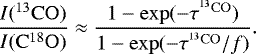
If the emission of the 13CO and C18O isotopologues is co-spatial, the line profiles are similar, and the gas ratio abundance 12CO:13CO:C18O is constant, then the 13CO optical depth can be assessed from the 13CO and C18O integrated intensity ratio I(13 CO)/I(C18O) using the formalism first described by Myers et al. (1983) and Ladd et al. (1998). The treatment employed here is adapted from Myers et al. (1983) and uses Eq. (A.1) (given by e.g. Carlhoff et al. 2013; Zhang et al. 2018), which relates the integrated intensity ratio of the two isotopologues (Table A.1) and the optical depth τ:
 (A.1)
(A.1)
In the above equation  is the 13CO optical depth and f is the intrinsic 13CO∕C18O abundance ratio, which is equal to 7−10 for the Milky Way (Wilson & Matteucci 1992; Barnes et al. 2015). If f = 8 is assumed, to be consistent with the approach adopted in Perotti et al. (2020),
  is equal to 1.22 for B35A−2, 0.39 for B35−3, 0.47 for B35A−5, and 0.03 for B35−4, indicating 13CO optically thick emission towards three (B35A−2, B35−3, and B35A−5) out of four sources in the B35A cloud as I(13 CO)/I(C18O) is below the intrinsic ratio f for these three sources. Thesame conclusion is obtained if f = 7 or f = 10 is assumed. Based on this result, the C18O emission was used to estimate the column densities of 12CO under LTE conditions.
A.3 Channel maps and spectra of individual transitions
Channel maps and spectra for the 13CO J = 2–1, C18 O J = 2–1, and CH3OH J = 50−40 A+ detected in the combined interferometric (SMA) and single-dish (IRAM 30 m/APEX) data are displayed in Figs. A.1 and A.3–A.5. The CO isotopologue emission is predominantly concentrated towards B35A−2 and B35A−3, whereas the CH3OH emission is uniquely localised in the vicinity of B35A−5. Blue-shifted components are observed in combination with broad spectral profiles and wings that deviate from the cloud velocity (12.42 km s−1).
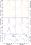 |
Fig. A.1 13CO J = 2−1, C18O J = 2−1, CH3OH J = 50−40 A+, and CH3OH J = 51−41 E− spectra towards the B35A sources detected in the combined interferometric and single-dish datasets. The spectra are colour-coded according to Fig. 7. The cloud velocity (12.42 km s−1) is shown in all spectra with a vertical grey line. |
Integrated 13CO and C18 O line intensities in units of Jy beam−1 km s−1 over each source position.
A.4 Derivation of gas-phase column densities
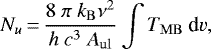
The column densities of gas-phase species towards the B35A sources were calculated using the integrated intensities of the combined interferometric (SMA) and single-dish (IRAM 30 m/APEX) data (Tables A.1 and A.2). The values inserted into the equations below are listed in Table 2 and have been taken from the Cologne Database for Molecular Spectroscopy (CDMS; Müller et al. 2001), Jet Propulsion Laboratory (JPL; Pickett et al. 1998), and Leiden Atomic and Molecular Database (LAMDA; Schöier et al. 2005) spectral databases. The adopted formalism assumes LTE conditions and, more specifically, optically thin line emission, homogeneous source filling the telescope beam, and level populations that can be described by a single excitation temperature. According to the treatment by Goldsmith & Langer (1999) and under the aforementioned conditions, the integrated main-beam temperature ∫ TMB dv and the column density Nu in the upper energy level u are related by:
 (A.2)
(A.2)
where kB is the Boltzmann constant, ν is the transition frequency, h is the Planck constant, c is the speed of light, and Aul is the spontaneous Einstein coefficient of the transition. The total column density Ntot and the rotational temperature Trot are related to the column density Nu in the upper energy level u (Goldsmith & Langer 1999) by:
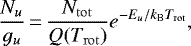 (A.3)
(A.3)
where gu is the upper level degeneracy, Q(Trot) is the rotational partition function, kB is the Boltzmann constant, and Eu is the energyof the upper level u. In summary, the column densities were calculated using the formalism of Goldsmith & Langer (1999) but assuming a fixed rotational temperatureequal to 25 K (Craigon 2015; Reipurth & Friberg 2021). Figure A.2 displays the rotational diagram of CH3OH for B35A−5. Only CH3OH transitions above 5σ were considered. The uncertainties on the gas column densities were estimated based on the rms noise of the spectra and on the ~20% calibration uncertainty.
Integrated CH3OH line intensities in units of Jy beam−1 km s−1 towards B35A−5.
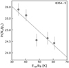 |
Fig. A.2 Rotational diagram of CH3OH for B35A−5. The solid line displays the fixed slope for Trot = 25 K. Error bars are for 1σ uncertainties. The derived column density is shown in Table 3. |
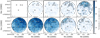 |
Fig. A.3 Channel maps for 13CO J = 2− 1 with velocityrange 6–16 km s−1 in channels of 1 km s−1. Contours start at 5σ and follow insteps of 5σ. |
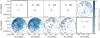 |
Fig. A.4 Channel maps for C18O J = 2− 1 with velocityrange 6–16 km s−1 in channels of 1 km s−1. Contours start at 5σ and follow insteps of 5σ. |
 |
Fig. A.5 Channel maps for CH3OH J = 50 − 40 A+ with velocityrange 6–16 km s−1 in channels of 1 km s−1. Contours start at 5σ and follow insteps of 5σ. |
Appendix B H2 column density from visual extinction
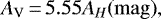
The production of the H2 column density map was accomplished by using the visual extinction (AV) values for B35A tabulated in the c2d catalogue6. No AV values are reported for B35A−2 or B35A−3 in the catalogue. As a result, the visual extinction for B35A−3 was retrieved by de-reddening its SED at the J, H, and K 2MASS photometricpoints of Table B.1 to fit a first blackbody and then fit a second blackbody to model the infrared excess at the IRAC photometric points (see Fig. B.1). The extinction in the H band (AH) was then calculated using the equation (Chapman et al. 2009):
![\begin{equation*} A_{\lambda}\,{=}\,{-}2.5~\mathrm{log} \left[ \left(\frac {F_{\lambda}} {B_{\lambda}} \right) \left(\frac {1} {\mathrm{k}} \right)\right],\end{equation*}](/articles/aa/full_html/2021/06/aa39669-20/aa39669-20-eq16.png) (B.1)
(B.1)
where λ is the wavelength corresponding in this case to the H band (1.662 μm), Fλ is the observed flux at the selected λ, k is a scaling factor, and Bλ is the blackbody function. The extinction in the H band was then converted to visual extinction using the equation:
 (B.2)
(B.2)
where the conversion factor is taken from Weingartner & Draine (2001). The adopted extinction law takes into account the dust model from Weingartner & Draine (2001) for RV = 5.5 designed for the dense ISM and used by the c2d collaboration (Chapman et al. 2009; Evans et al. 2009). No NIR photometry data are available for B35A−2, and thus the AV for this source was obtained by interpolating all the tabulated visual extinction values for B35A taken from the c2d catalogue, including the AV value for B35A−3. The obtained visual extinction map of B35A was then converted to an H2 column density map using the relation established for dense ISM gas (Evans et al. 2009):
 (B.3)
(B.3)
Photometry of B35A−3.
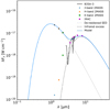 |
Fig. B.1 SED of B35A−3, which was modelled to determine its visual extinction. The dotted and dashed lines represent the blackbody functions used to model the stellar component and the infrared excess, respectively. The solid line is the sum of the two contributions. |
References
- Acharyya, K., Fuchs, G. W., Fraser, H. J., van Dishoeck, E. F., & Linnartz, H. 2007, A&A, 466, 1005 [NASA ADS] [CrossRef] [EDP Sciences] [Google Scholar]
- Allen, V., Cordiner, M., & Charnley, S. 2020, ArXiv e-prints [arXiv:2010.01151] [Google Scholar]
- Ansdell, M., Haworth, T. J., Williams, J. P., et al. 2020, AJ, 160, 248 [Google Scholar]
- Barnes, P. J., Muller, E., Indermuehle, B., et al. 2015, ApJ, 812, 6 [Google Scholar]
- Barrado, D., Stelzer, B., Morales-Calderón, M., et al. 2011, A&A, 526, A21 [NASA ADS] [CrossRef] [EDP Sciences] [Google Scholar]
- Barrado, D., de Gregorio Monsalvo, I., Huélamo, N., et al. 2018, A&A, 612, A79 [CrossRef] [EDP Sciences] [Google Scholar]
- Bayo, A., Barrado, D., Stauffer, J., et al. 2011, A&A, 536, A63 [NASA ADS] [CrossRef] [EDP Sciences] [Google Scholar]
- Bergin, E. A.,& Tafalla, M. 2007, ARA&A, 45, 339 [Google Scholar]
- Bergner, J. B., Öberg, K. I., Garrod, R. T., & Graninger, D. M. 2017, ApJ, 841, 120 [NASA ADS] [CrossRef] [Google Scholar]
- Bertin, M., Romanzin, C., Doronin, M., et al. 2016, ApJ, 817, L12 [Google Scholar]
- Bisschop, S. E., Fraser, H. J., Öberg, K. I., van Dishoeck, E. F., & Schlemmer, S. 2006, A&A, 449, 1297 [NASA ADS] [CrossRef] [EDP Sciences] [Google Scholar]
- Bjerkeli, P., Liseau, R., Larsson, B., et al. 2012, A&A, 546, A29 [NASA ADS] [CrossRef] [EDP Sciences] [Google Scholar]
- Bjerkeli, P., Jørgensen, J. K., Bergin, E. A., et al. 2016, A&A, 595, A39 [NASA ADS] [CrossRef] [EDP Sciences] [Google Scholar]
- Blanksby, S., & Ellison, G. 2003, Acc. Chem. Res., 36, 255 [CrossRef] [PubMed] [Google Scholar]
- Boogert, A. C. A., Gerakines, P. A., & Whittet, D. C. B. 2015, ARA&A, 53, 541 [Google Scholar]
- Buckle, J. V., Hills, R. E., Smith, H., et al. 2009, MNRAS, 399, 1026 [NASA ADS] [CrossRef] [Google Scholar]
- Calcutt, H., Jørgensen, J. K., Müller, H. S. P., et al. 2018, A&A, 616, A90 [NASA ADS] [CrossRef] [EDP Sciences] [Google Scholar]
- Carlhoff, P., Nguyen Luong, Q., Schilke, P., et al. 2013, A&A, 560, A24 [NASA ADS] [CrossRef] [EDP Sciences] [Google Scholar]
- Cazaux, S., Tielens, A. G. G. M., Ceccarelli, C., et al. 2003, ApJ, 593, L51 [NASA ADS] [CrossRef] [Google Scholar]
- Cazaux, S., Minissale, M., Dulieu, F., & Hocuk, S. 2016, A&A, 585, A55 [NASA ADS] [CrossRef] [EDP Sciences] [Google Scholar]
- Cazaux, S., Martín-Doménech, R., Chen, Y. J., Muñoz Caro, G. M., & González Díaz C. 2017, ApJ, 849, 80 [Google Scholar]
- Chandler, C. J., & Carlstrom, J. E. 1996, ApJ, 466, 338 [NASA ADS] [CrossRef] [Google Scholar]
- Chapman, N. L., Mundy, L. G., Lai, S.-P., & Evans, II, N. J. 2009, ApJ, 690, 496 [NASA ADS] [CrossRef] [Google Scholar]
- Collings, M. P., Anderson, M. A., Chen, R., et al. 2004, MNRAS, 354, 1133 [NASA ADS] [CrossRef] [Google Scholar]
- Connelley, M. S., Reipurth, B., & Tokunaga, A. T. 2008, AJ, 135, 2496 [NASA ADS] [CrossRef] [Google Scholar]
- Conti, P. S., & Leep, E. M. 1974, ApJ, 193, 113 [NASA ADS] [CrossRef] [Google Scholar]
- Craigon, A. M. 2015, PhD thesis, University of Strathclyde, UK [Google Scholar]
- Cruz-Diaz, G. A., Martín-Doménech, R., Muñoz Caro, G. M., & Chen, Y.-J. 2016, A&A, 592, A68 [NASA ADS] [CrossRef] [EDP Sciences] [Google Scholar]
- Cuppen, H. M., Penteado, E. M., Isokoski, K., van der Marel, N., & Linnartz, H. 2011, MNRAS, 417, 2809 [NASA ADS] [CrossRef] [Google Scholar]
- Dartois, E., Chabot, M., Id Barkach, T., et al. 2019, A&A, 627, A55 [NASA ADS] [CrossRef] [EDP Sciences] [Google Scholar]
- Dartois, E., Chabot, M., Bacmann, A., et al. 2020, A&A, 634, A103 [NASA ADS] [CrossRef] [EDP Sciences] [Google Scholar]
- De Vries, C. H., Narayanan, G., & Snell, R. L. 2002, ApJ, 577, 798 [NASA ADS] [CrossRef] [Google Scholar]
- Dempsey, J. T., Friberg, P., Jenness, T., et al. 2013, MNRAS, 430, 2534 [Google Scholar]
- Di Francesco, J., Johnstone, D., Kirk, H., MacKenzie, T., & Ledwosinska, E. 2008, ApJS, 175, 277 [NASA ADS] [CrossRef] [Google Scholar]
- Dionatos, O., Jørgensen, J. K., Green, J. D., et al. 2013, A&A, 558, A88 [NASA ADS] [CrossRef] [EDP Sciences] [Google Scholar]
- Dolan, C. J., & Mathieu, R. D. 1999, AJ, 118, 2409 [NASA ADS] [CrossRef] [Google Scholar]
- Dolan, C. J., & Mathieu, R. D. 2002, AJ, 123, 387 [NASA ADS] [CrossRef] [Google Scholar]
- Dulieu, F., Congiu, E., Noble, J., et al. 2013, Sci. Rep., 3, 1338 [NASA ADS] [CrossRef] [Google Scholar]
- Eistrup, C., Walsh, C., & van Dishoeck, E. F. 2016, A&A, 595, A83 [NASA ADS] [CrossRef] [EDP Sciences] [Google Scholar]
- Evans, II, N. J., Dunham, M. M., Jørgensen, J. K., et al. 2009, ApJS, 181, 321 [NASA ADS] [CrossRef] [Google Scholar]
- Evans, II, N. J., Allen, L. E., Blake, G. A., et al. 2014, VizieR Online Data Catalog: II/332 [Google Scholar]
- Fraser, H. J., & van Dishoeck, E. F. 2004, Adv. Space Res., 33, 14 [Google Scholar]
- Fraser, H. J., Collings, M. P., McCoustra, M. R. S., & Williams, D. A. 2001, MNRAS, 327, 1165 [NASA ADS] [CrossRef] [Google Scholar]
- Garrod, R., Park, I. H., Caselli, P., & Herbst, E. 2006, Faraday Discuss., 133, 51 [NASA ADS] [CrossRef] [PubMed] [Google Scholar]
- Goldsmith, P. F., & Langer, W. D. 1999, ApJ, 517, 209 [Google Scholar]
- Grassi, T., Bovino, S., Caselli, P., et al. 2020, A&A, 643, A155 [EDP Sciences] [Google Scholar]
- Griffin, M. J., Abergel, A., Abreu, A., et al. 2010, A&A, 518, L3 [EDP Sciences] [Google Scholar]
- Güsten, R., Nyman, L. Å., Schilke, P., et al. 2006, A&A, 454, L13 [NASA ADS] [CrossRef] [EDP Sciences] [Google Scholar]
- Heiles, C., & Habing, H. J. 1974, A&AS, 14, 1 [NASA ADS] [Google Scholar]
- Herbst, E., & van Dishoeck, E. F. 2009, ARA&A, 47, 427 [NASA ADS] [CrossRef] [Google Scholar]
- Hernández, J., Calvet, N., Hartmann, L., et al. 2009, ApJ, 707, 705 [NASA ADS] [CrossRef] [Google Scholar]
- Ho, P. T. P., Moran, J. M., & Lo, K. Y. 2004, ApJ, 616, L1 [NASA ADS] [CrossRef] [Google Scholar]
- Hollenbach, D., & McKee, C. F. 1989, ApJ, 342, 306 [NASA ADS] [CrossRef] [Google Scholar]
- Jiménez-Serra, I., Caselli, P., Martín-Pintado, J., & Hartquist, T. W. 2008, A&A, 482, 549 [NASA ADS] [CrossRef] [EDP Sciences] [Google Scholar]
- Jørgensen, J. K., Hogerheijde, M. R., Blake, G. A., et al. 2004, A&A, 415, 1021 [NASA ADS] [CrossRef] [EDP Sciences] [Google Scholar]
- Jørgensen, J. K., van der Wiel, M. H. D., Coutens, A., et al. 2016, A&A, 595, A117 [NASA ADS] [CrossRef] [EDP Sciences] [Google Scholar]
- Jørgensen, J. K., Belloche, A., & Garrod, R. T. 2020, ARA&A, 58, 727 [Google Scholar]
- Kauffmann, J., Bertoldi, F., Bourke, T. L., Evans, II, N. J., & Lee, C. W. 2008, A&A, 487, 993 [NASA ADS] [CrossRef] [EDP Sciences] [Google Scholar]
- Kounkel, M. 2020, ApJ, 902, 122 [NASA ADS] [CrossRef] [Google Scholar]
- Kounkel, M., Covey, K., Suárez, G., et al. 2018, AJ, 156, 84 [NASA ADS] [CrossRef] [Google Scholar]
- Kristensen, L. E., van Dishoeck, E. F., van Kempen, T. A., et al. 2010, A&A, 516, A57 [NASA ADS] [CrossRef] [EDP Sciences] [Google Scholar]
- Lada, C. J., & Black, J. H. 1976, ApJ, 203, L75 [Google Scholar]
- Ladd, E. F., Fuller, G. A., & Deane, J. R. 1998, ApJ, 495, 871 [Google Scholar]
- Lang, W. J., Masheder, M. R. W., Dame, T. M., & Thaddeus, P. 2000, A&A, 357, 1001 [NASA ADS] [Google Scholar]
- Lee, H.-T., Chen, W. P., Zhang, Z.-W., & Hu, J.-Y. 2005, ApJ, 624, 808 [NASA ADS] [CrossRef] [Google Scholar]
- Maddalena, R. J., & Morris, M. 1987, ApJ, 323, 179 [NASA ADS] [CrossRef] [Google Scholar]
- Manigand, S., Jørgensen, J. K., Calcutt, H., et al. 2020, A&A, 635, A48 [NASA ADS] [CrossRef] [EDP Sciences] [Google Scholar]
- Martín-Doménech, R., Muñoz Caro, G. M., & Cruz-Díaz, G. A. 2016, A&A, 589, A107 [NASA ADS] [CrossRef] [EDP Sciences] [Google Scholar]
- Mathieu, R. D. 2008, ASP Monographs, 4, 757 [Google Scholar]
- McGuire, B. A. 2018, ApJS, 239, 17 [Google Scholar]
- McMullin, J. P., Waters, B., Schiebel, D., Young, W., & Golap, K. 2007, ASP Conf. Ser., 376, 127 [Google Scholar]
- Morgan, L. K., Thompson, M. A., Urquhart, J. S., & White, G. J. 2008, A&A, 477, 557 [NASA ADS] [CrossRef] [EDP Sciences] [Google Scholar]
- Müller, H. S. P., Thorwirth, S., Roth, D. A., & Winnewisser, G. 2001, A&A, 370, L49 [NASA ADS] [CrossRef] [EDP Sciences] [Google Scholar]
- Murdin, P., & Penston, M. V. 1977, MNRAS, 181, 657 [NASA ADS] [CrossRef] [Google Scholar]
- Myers, P. C., Linke, R. A., & Benson, P. J. 1983, ApJ, 264, 517 [NASA ADS] [CrossRef] [Google Scholar]
- Myers, P. C., Heyer, M., Snell, R. L., & Goldsmith, P. F. 1988, ApJ, 324, 907 [NASA ADS] [CrossRef] [Google Scholar]
- Neufeld, D. A., & Dalgarno, A. 1989, ApJ, 340, 869 [Google Scholar]
- Nisini, B., Benedettini, M., Codella, C., et al. 2010, A&A, 518, L120 [NASA ADS] [CrossRef] [EDP Sciences] [Google Scholar]
- Noble, J. A., Congiu, E., Dulieu, F., & Fraser, H. J. 2012, MNRAS, 421, 768 [NASA ADS] [Google Scholar]
- Noble, J. A., Fraser, H. J., Aikawa, Y., Pontoppidan, K. M., & Sakon, I. 2013, ApJ, 775, 85 [NASA ADS] [CrossRef] [Google Scholar]
- Noble, J. A., Fraser, H. J., Pontoppidan, K. M., & Craigon, A. M. 2017, MNRAS, 467, 4753 [CrossRef] [Google Scholar]
- Öberg, K. I. 2016, Chem. Rev., 116, 9631 [Google Scholar]
- Öberg, K. I., & Bergin, E. A. 2021, Phys. Rep., 893, 1 [Google Scholar]
- Öberg, K. I., Bottinelli, S., & van Dishoeck, E. F. 2009, A&A, 494, L13 [NASA ADS] [CrossRef] [EDP Sciences] [Google Scholar]
- Öberg, K. I., Murray-Clay, R., & Bergin, E. A. 2011, ApJ, 743, L16 [NASA ADS] [CrossRef] [Google Scholar]
- Ossenkopf, V.,& Henning, T. 1994, A&A, 291, 943 [Google Scholar]
- Penteado, E. M., Walsh, C., & Cuppen, H. M. 2017, ApJ, 844, 71 [NASA ADS] [CrossRef] [Google Scholar]
- Perotti, G., Rocha, W. R. M., Jørgensen, J. K., et al. 2020, A&A, 643, A48 [EDP Sciences] [Google Scholar]
- Pickett, H. M., Poynter, R. L., Cohen, E. A., et al. 1998, J. Quant. Spectr. Rad. Transf, 60, 883 [Google Scholar]
- Qin, S.-L., & Wu, Y.-F. 2003, Chinese J. Astron. Astrophys., 3, 69 [Google Scholar]
- Rabli, D., & Flower, D. R. 2010, MNRAS, 406, 95 [Google Scholar]
- Reipurth, B. 2000, VizieR Online Data Catalog: V/104 [Google Scholar]
- Reipurth, B., & Bally, J. 2001, ARA&A, 39, 403 [NASA ADS] [CrossRef] [Google Scholar]
- Reipurth, B., & Friberg, P. 2021, MNRAS, 501, 5938 [Google Scholar]
- Sahan, M., & Haffner, L. M. 2016, AJ, 151, 147 [Google Scholar]
- Santangelo, G., Nisini, B., Giannini, T., et al. 2012, A&A, 538, A45 [NASA ADS] [CrossRef] [EDP Sciences] [Google Scholar]
- Schöier, F. L., van der Tak, F. F. S., van Dishoeck, E. F., & Black, J. H. 2005, A&A, 432, 369 [NASA ADS] [CrossRef] [EDP Sciences] [Google Scholar]
- Sharpless, S. 1959, ApJS, 4, 257 [Google Scholar]
- Skrutskie, M. F., Cutri, R. M., Stiening, R., et al. 2006, AJ, 131, 1163 [NASA ADS] [CrossRef] [Google Scholar]
- Suutarinen, A. 2015, PhD thesis, The Open University, UK [Google Scholar]
- Suutarinen, A. N., Kristensen, L. E., Mottram, J. C., Fraser, H. J., & van Dishoeck, E. F. 2014, MNRAS, 440, 1844 [NASA ADS] [CrossRef] [Google Scholar]
- van Dishoeck, E. F., & Blake, G. A. 1998, ARA&A, 36, 317 [NASA ADS] [CrossRef] [Google Scholar]
- van ’t, M. L. R., Walsh, C., Kama, M., Facchini, S., & van Dishoeck, E. F. 2017, A&A, 599, A101 [NASA ADS] [CrossRef] [EDP Sciences] [Google Scholar]
- van Gelder, M. L., Tabone, B., Tychoniec, Ł., et al. 2020, A&A, 639, A87 [CrossRef] [EDP Sciences] [Google Scholar]
- Vasta, M., Codella, C., Lorenzani, A., et al. 2012, A&A, 537, A98 [NASA ADS] [CrossRef] [EDP Sciences] [Google Scholar]
- Vasyunin, A. I., & Herbst, E. 2013, ApJ, 769, 34 [Google Scholar]
- Wade, C. M. 1957, AJ, 62, 148 [NASA ADS] [CrossRef] [Google Scholar]
- Watanabe, N., & Kouchi, A. 2002, ApJ, 571, L173 [Google Scholar]
- Weingartner, J. C., & Draine, B. T. 2001, ApJ, 548, 296 [Google Scholar]
- Whittet, D. C. B., Cook, A. M., Herbst, E., Chiar, J. E., & Shenoy, S. S. 2011, ApJ, 742, 28 [NASA ADS] [CrossRef] [Google Scholar]
- Wilson, T. L. 1999, Rep. Prog. Phys., 62, 143 [Google Scholar]
- Wilson, T. L., & Matteucci, F. 1992, A&ARv, 4, 1 [NASA ADS] [CrossRef] [Google Scholar]
- Wolfire, M. G., Hollenbach, D., & Tielens, A. G. G. M. 1989, ApJ, 344, 770 [NASA ADS] [CrossRef] [Google Scholar]
- Yang, B., Stancil, P. C., Balakrishnan, N., & Forrey, R. C. 2010, ApJ, 718, 1062 [NASA ADS] [CrossRef] [Google Scholar]
- Zhang, C. Y., Laureijs, R. J., Chlewicki, G., Clark, F. O., & Wesselius, P. R. 1989, A&A, 218, 231 [Google Scholar]
- Zhang, Z.-Y., Romano, D., Ivison, R. J., Papadopoulos, P. P., & Matteucci, F. 2018, Nature, 558, 260 [Google Scholar]
- Zucker, C., Speagle, J. S., Schlafly, E. F., et al. 2019, ApJ, 879, 125 [NASA ADS] [CrossRef] [Google Scholar]
- Zucker, C., Speagle, J. S., Schlafly, E. F., et al. 2020, A&A, 633, A51 [CrossRef] [EDP Sciences] [Google Scholar]
All Tables
Integrated 13CO and C18 O line intensities in units of Jy beam−1 km s−1 over each source position.
All Figures
|
Fig. 1 Three-colour image of B35A overlaid with SCUBA−2 850 μm density flux in units of mJy beam−1 (Reipurth & Friberg 2021); contours are in decreasing steps of 30% starting at 7.3 Jy beam−1. The composite is made from Spitzer IRAC 3.6 μm (blue), 4.5 μm (green), and Multiband Imaging Photometer for Spitzer (MIPS) 24.0 μm (red) bands (programme ID: 139, PI: N. J. Evans II). The white stars mark the positions of the AKARI and Spitzer c2d identified B35A sources. Connelley et al. (2008) and Reipurth & Friberg (2021) show the B35A sources to be multiplet systems totalling four or five objects. |
| In the text | |
|
Fig. 2 Integrated intensity maps for 13CO J = 2−1 detected by the SMA (panel a), by the IRAM 30 m telescope (panel b), and in the combined interferometric SMA and single-dish IRAM 30 m data (panel c). All lines are integrated between 7 and 16 km s−1. Contours are at 5σ, 10σ, 15σ, etc. (σSMA = 0.42 Jy beam−1 km s−1, σIRAM 30 m = 6 Jy beam−1 km s−1, σSMA+IRAM 30 m = 1.03 Jy beam−1 km s−1). Panel c: white area outlines the primary beam of the SMA observations. The synthesised beams are displayed in white in the bottom left corner of each panel. The white stars mark the positions of the targeted B35A sources. |
| In the text | |
|
Fig. 3 Integrated intensity maps for C18O J = 2 detected by the SMA (panel a), by the IRAM 30 m telescope (panel b), and in the combined interferometric SMA and single-dish IRAM 30 m data (panel c). All lines are integrated between 10 and 15 km s−1. Contours are at 5, 10, and 15σ (σSMA = 0.37 Jy beam−1 km s−1, σIRAM 30 m = 5 Jy beam−1 km s−1, σSMA+IRAM 30 m = 0.40 Jy beam−1 km s−1). Panel c: white area outlines the primary beam of the SMA observations. The synthesised beams are displayed in white in the bottom left corner of each panel. The white stars mark the positions of the targeted B35A sources. |
| In the text | |
|
Fig. 4 Integrated intensity maps for CH3OH J = 50–40 A+ detected by the SMA (panel a), by the APEX telescope (panel b), and in the combined interferometric SMA and single-dish APEX data (panel c). All lines are integrated between 6 and 12.5 km s−1. Contours start at 5σ (σSMA = 0.04 Jy beam−1 km s−1, σAPEX = 4 Jy beam−1 km s−1, σSMA+APEX = 0.04 Jy beam−1 km s−1) and follow insteps of 5σ. Panel c: white area outlines the primary beam of the SMA observations. The synthesised beams are displayed in white in the bottom left corner of each panel. The white stars mark the positions of the targeted B35A sources, and the dotted blue line indicates the direction of the giant outflow terminating at HH 175. |
| In the text | |
|
Fig. 5 H2 column density maps of B35A. a:
|
| In the text | |
|
Fig. 6 Gas-ice maps of B35A. Ice abundances are indicated as filled grey (panels a and b) or white circles (panels c and d), and upper limits are displayed as empty circles. Contour levels are 5, 10, and 15σ. a: CO ice abundances on gas 13CO 2−1. b: CO ice abundances on gas C18O 2−1. c: CH3OH ice abundances on gas CH3OH 50−40 A+. d: H2O ice abundances on gas CH3OH 50−40 A+. The white area outlines the primary beam of the SMA observations. The white stars mark the positions of the targeted B35A sources. |
| In the text | |
|
Fig. 7 Gas and ice variations in B35A. The circles represent the targeted B35A sources. Panels a–c: relation between CO, CH3OH, and H2O ice and CO gas abundances relative to H2. |
| In the text | |
|
Fig. 8 H2O (top), CO (middle), and CH3OH (bottom) total ice column densities obtained in Suutarinen (2015, the sources are colour-coded) compared to Noble et al. (2017, light grey). The empty bars represent upper limits on the column densities. |
| In the text | |
|
Fig. 9 CH3OH (panel a) and CO (panel b) gas-to-ice ratios (Ngas/Nice) for the multiple protostellar system in Orion B35A and Serpens SVS 4. The dark green squares indicate the gas-to-ice ratios estimated by Perotti et al. (2020) for the Serpens SVS 4 cluster. The light green circles mark the ratios calculated in this study. The dotted light blue line in panel a represents the ratio estimated by Öberg et al. (2009) towards Class 0/I objects. The shaded areas indicate the estimated ranges of the gas-to-ice ratios. |
| In the text | |
|
Fig. A.1 13CO J = 2−1, C18O J = 2−1, CH3OH J = 50−40 A+, and CH3OH J = 51−41 E− spectra towards the B35A sources detected in the combined interferometric and single-dish datasets. The spectra are colour-coded according to Fig. 7. The cloud velocity (12.42 km s−1) is shown in all spectra with a vertical grey line. |
| In the text | |
|
Fig. A.2 Rotational diagram of CH3OH for B35A−5. The solid line displays the fixed slope for Trot = 25 K. Error bars are for 1σ uncertainties. The derived column density is shown in Table 3. |
| In the text | |
|
Fig. A.3 Channel maps for 13CO J = 2− 1 with velocityrange 6–16 km s−1 in channels of 1 km s−1. Contours start at 5σ and follow insteps of 5σ. |
| In the text | |
|
Fig. A.4 Channel maps for C18O J = 2− 1 with velocityrange 6–16 km s−1 in channels of 1 km s−1. Contours start at 5σ and follow insteps of 5σ. |
| In the text | |
|
Fig. A.5 Channel maps for CH3OH J = 50 − 40 A+ with velocityrange 6–16 km s−1 in channels of 1 km s−1. Contours start at 5σ and follow insteps of 5σ. |
| In the text | |
|
Fig. B.1 SED of B35A−3, which was modelled to determine its visual extinction. The dotted and dashed lines represent the blackbody functions used to model the stellar component and the infrared excess, respectively. The solid line is the sum of the two contributions. |
| In the text | |
Current usage metrics show cumulative count of Article Views (full-text article views including HTML views, PDF and ePub downloads, according to the available data) and Abstracts Views on Vision4Press platform.
Data correspond to usage on the plateform after 2015. The current usage metrics is available 48-96 hours after online publication and is updated daily on week days.
Initial download of the metrics may take a while.