| Issue |
A&A
Volume 648, April 2021
|
|
|---|---|---|
| Article Number | L3 | |
| Number of page(s) | 12 | |
| Section | Letters to the Editor | |
| DOI | https://doi.org/10.1051/0004-6361/202140642 | |
| Published online | 07 April 2021 | |
Letter to the Editor
TMC-1, the starless core sulfur factory: Discovery of NCS, HCCS, H2CCS, H2CCCS, and C4S and detection of C5S⋆
1
Grupo de Astrofísica Molecular, Instituto de Física Fundamental (IFF-CSIC), C/ Serrano 121, 28006 Madrid, Spain
e-mail: This email address is being protected from spambots. You need JavaScript enabled to view it.
2
Observatorio Astronómico Nacional (IGN), C/ Alfonso XII, 3, 28014 Madrid, Spain
3
Centro de Desarrollos Tecnológicos, Observatorio de Yebes (IGN), 19141 Yebes, Guadalajara, Spain
Received:
23
February
2021
Accepted:
17
March
2021
Abstract
We report the detection of the sulfur-bearing species NCS, HCCS, H2CCS, H2CCCS, and C4S for the first time in space. These molecules were found towards TMC-1 through the observation of several lines for each species. We also report the detection of C5S for the first time in a cold cloud through the observation of five lines in the 31–50 GHz range. The derived column densities are N(NCS) = (7.8 ± 0.6) × 1011 cm−2, N(HCCS) = (6.8 ± 0.6) × 1011 cm−2, N(H2CCS) = (7.8 ± 0.8) × 1011 cm−2, N(H2CCCS) = (3.7 ± 0.4) × 1011 cm−2, N(C4S) = (3.8 ± 0.4) × 1010 cm−2, and N(C5S) = (5.0 ± 1.0) × 1010 cm−2. The observed abundance ratio between C3S and C4S is 340, that is to say a factor of approximately one hundred larger than the corresponding value for CCS and C3S. The observational results are compared with a state-of-the-art chemical model, which is only partially successful in reproducing the observed abundances. These detections underline the need to improve chemical networks dealing with S-bearing species.
Key words: astrochemistry / ISM: molecules / ISM: individual objects: TMC-1 / line: identification / molecular data
Based on observations carried out with the Yebes 40 m telescope (projects 19A003, 20A014, and 20D023) and the Institut de Radioastronomie Millimétrique (IRAM) 30 m telescope. The 40 m radiotelescope at Yebes Observatory is operated by the Spanish Geographic Institute (IGN, Ministerio de Transportes, Movilidad y Agenda Urbana). IRAM is supported by INSU/CNRS (France), MPG (Germany), and IGN (Spain).
© ESO 2021
1. Introduction
The cold dark core TMC-1 presents an interesting carbon-rich chemistry that leads to the formation of long neutral carbon-chain radicals and their anions, as well as cyanopolyynes (see Cernicharo et al. 2020a,b and references therein). The carbon chains CCS and CCCS are particularly abundant in this cloud (Saito et al. 1987; Yamamoto et al. 1987) and also exist in the envelopes of carbon-rich circumstellar envelopes (Cernicharo et al. 1987). TMC-1 is also peculiar due to the presence of protonated species of abundant large carbon chains such as HC3O+ (Cernicharo et al. 2020c), HC5NH+ (Marcelino et al. 2020), HC3S+ (Cernicharo et al. 2021a), and CH3CO+ (Cernicharo et al. 2021b). The number of sulfur-bearing species detected to date in TMC-1 is small compared to oxygen- and nitrogen-bearing species (see, e.g. McGuire et al. 2019). In fact, the chemistry of sulfur-bearing molecules is strongly dependent on the depletion of sulfur (Vidal et al. 2017). Many reactions involving S+ with neutrals as well as radicals with S and CS have to be studied to achieve a better chemical modelling of sulfur-bearing species (Petrie 1996; Bulut et al. 2021). Nevertheless, the main input to understand these chemical processes is to unveil new sulfur-bearing species in the interstellar medium as well as to understand their formation paths and their role in the chemistry of sulfur.
In this Letter we report the discovery, for the first time in space, of the following five new sulfur-bearing species: NCS, HCCS, H2CCS, H2CCCS, and C4S. The detection of C5S in a cold dark cloud is also reported for the first time. A detailed observational study of the most relevant S-bearing species in this cloud is accomplished. We discuss these results in the context of state-of-the-art chemical models.
2. Observations
New receivers, built within the Nanocosmos project1, and installed at the Yebes 40 m radio telescope were used for the observations of TMC-1. The receivers and the spectrometers have been described by Tercero et al. (2021). The observations needed to complete the Q-band line survey towards TMC-1 (αJ2000 = 4h41m41.9s and δJ2000 = +25° 41′27.0″) were performed in several sessions during December 2019 and January 2021. All data were analysed using the GILDAS package2. The observing procedure has been previously described (see, e.g. Cernicharo et al. 2021a,b). The IRAM 30 m data come from a line survey performed towards TMC-1 and B1 and the observations have been described by Marcelino et al. (2007) and Cernicharo et al. (2013).
The intensity scale, antenna temperature ( ) was calibrated using two absorbers at different temperatures and an atmospheric transmission model (ATM; Cernicharo 1985; Pardo et al. 2001). Calibration uncertainties have been adopted to be 10%. The nominal spectral resolution of 38.15 kHz was used for the final spectra.
3. Results and discussion
Line identification in our TMC-1 survey has been performed using the MADEX catalogue (Cernicharo 2012), the Cologne Database of Molecular Spectroscopy catalogue (Müller et al. 2005), and the JPL catalogue (Pickett et al. 1998). A description of the methods used to fit the data and to derive column densities is provided in Appendix A.
3.1. HCCS and NCS
Among the unidentified spectral features, we have found a couple separated by 1 MHz that perfectly match the frequencies of the strongest hyperfine components of the J = 7/2–5/2 transition of HCCS (2Π3/2). This species was observed in the laboratory by Kim et al. (2002) and the prediction of its rotational spectrum is available in the CDMS (Müller et al. 2005) and MADEX (Cernicharo 2012) catalogues. Taking into account the perfect match in frequencies, the narrow linewidth of the emission features in this source, and the perfect match in the relative intensities of the two hyperfine components, the possibility of a fortuitous coincidence is very low. Hence, we conclude that these two lines arise from HCCS. The observed lines are shown in Fig. 1 and the derived line parameters are given in Table D.1. The synthetic spectrum on Fig. 1 corresponds to Tr = 5 K and N(HCCS) = 6.8 × 1011 cm−2. We searched for HCCCS but only a 3σ upper limit to its column density of 2.4 × 1011 cm−2 can be given (see Table 1).
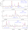 |
Fig. 1. Observed lines of HCCS (panel a) and NCS (panels b and c) towards TMC-1. The abscissa corresponds to the rest frequency assuming a local standard of rest velocity of the source of 5.83 km s−1 (see text). Blanked channels correspond to negative features produced in the frequency switching data folding. The ordinate is the antenna temperature corrected for atmospheric and telescope losses in milliKelvin. Spectral resolution is 38.15 kHz. The red lines show the synthetic spectrum of HCCS and NCS for a rotational temperature of 5 K, a linewidth of 0.6 km s−1, and a column density of 6.8 × 1011 cm−2 and 7.8 × 1011 cm−2, respectively. |
Column densities of sulfur-bearing species in TMC-1.
Thiocyanogen, NCS, has been observed in the laboratory (Amano & Takako 1991; McCarthy et al. 2003; Maeda et al. 2007), but never detected in space. Only one rotational transition lies within the Q-band, the J = 5/2–3/2 transition of NCS in its 2Π3/2 ladder. Figure 1 shows the three hyperfine components of this transition observed in TMC-1. The match between observations and the synthetic spectrum, corresponding to Tr = 5 K and N(NCS) = 7.8 × 1011 cm−2, is remarkably good, ensuring the discovery of this sulfur compound in TMC-1. The oxygen analogue of thiocyanogen, the isocyanate radical (NCO), was detected in cold core L483 by Marcelino et al. (2018). Unfortunately, NCO does not have lines in the 31–50 GHz range.
3.2. H2CCS and H2CCCS
Prompted by the detection of HCCS, we searched for other sulfur-bearing species in our survey. McGuire et al. (2019) searched for H2CCS, thioketene, in TMC-1. They obtained an upper limit to its column density of 5.5 × 1012 cm−2. Unfortunately they used a transition with an upper level energy around 40 K, which is not the best for the physical conditions of TMC-1. In this work we report the discovery of thioketene in space through observations of transitions with smaller upper level energies.
Spectroscopic laboratory data of thioketene (Georgiou et al. 1979; Winnewiser & Schäfer 1980; McNaughton et al. 1996) and H2CCCS (Brown et al. 1988) were used to predict the frequencies of these species and implement them in the MADEX code. The dipole moments adopted for H2CCS and H2CCCS are 1.02 D (Georgiou et al. 1979) and 2.06 D (Brown et al. 1988), respectively. We detected the four ortho and two para transitions of H2CCS expected in our data, as shown in Fig. 2. For H2CCCS (propadienthione), six ortho and three para transitions are detected (see seven of them in Fig. 3). The derived line parameters for both species are given in Table D.1.
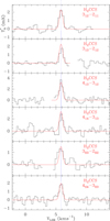 |
Fig. 2. Observed transitions of H2CCS towards TMC-1. The abscissa corresponds to the velocity in km s−1 of the source with respect to the local standard of rest. Line parameters are given in Table D.1. The ordinate is the antenna temperature corrected for atmospheric and telescope losses in milliKelvin. Blanked channels correspond to negative features produced by the folding of the frequency switching observations. The vertical blue dashed line indicates the vLSR of the cloud (5.83 km s−1). The red line spectra correspond to the synthetic model spectrum for each line adopting Tr = 7 K, N(o-H2CCS) = 6.0 × 1011 cm−2, and N(p-H2CCS) = 1.8 × 1011 cm−2 (see text). |
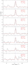 |
Fig. 3. Selected transitions of H2CCCS towards TMC-1. The abscissa corresponds to the velocity in km s−1 of the source with respect to the local standard of rest. Line parameters are given in Table D.1. The ordinate is the antenna temperature corrected for atmospheric and telescope losses in milliKelvin. Blanked channels correspond to negative features produced by the folding of the frequency switching observations. The vertical blue dashed line indicates the vLSR of the cloud (5.83 km s−1). The red line spectra correspond to the synthetic model of the emission obtained for Tr = 10 K, N(o-H2CCS) = 3.0 × 1011 cm−2, and N(p-H2CCS) = 6.5 × 1010 cm−2. |
An analysis of the data through a standard rotation diagram provides rotational temperatures of 7 ± 1 K and 10 ± 1 K for H2CCS and H2CCCS, respectively. For H2CCS, we derived N(ortho) = (6.0 ± 0.6) × 1011 cm−2, and N(para) = (1.8 ± 0.2) × 1011 cm−2. Hence, the ortho/para ratio for this species is 3.3 ± 0.7. For H2CCCS, we derived N(ortho) = (3.0 ± 0.3) × 1011 cm−2, and N(para) = (6.5 ± 0.5) × 1010 cm−2, respectively. The ortho/para abundance ratio derived for this species is 4.6 ± 0.8. These ortho/para ratios are compatible with the 3/1 value expected from the statitiscal spin degeneracies. They imply that non-significant enrichment of the para species is produced through reactions of H2CCS and H2CCCS with  , or other protonated molecular cations. The synthetic spectrum computed with these parameters for both species is shown in red in the different panels of Figs. 2 and 3. The derived abundance ratio between H2CCS and H2CCCS is ≃2, which is very different from the H2CCO/H2CCCO abundance ratio of > 130 derived in the same source by Cernicharo et al. (2020c), but very similar to the C2S/C3S abundance ratio of ∼3 derived here (see Table 1).
3.3. C4S and C5S
Taking the large column density derived for CCS and C3S into account (Cernicharo et al. 2021a), the next member of this family, C4S, is a potential candidate to be present in TMC-1. The spectroscopic laboratory data used to predict the spectrum of C4S are from Hirahara et al. (1993) and Gordon et al. (2001). A dipole moment of 4.03 D was computed through ab initio calculations by Pascoli & Lavendy (1998) and Lee (1997). Nineteen transitions of this species have frequencies within the range of our line survey. The line by line search through our data provides a clear detection for the Nu = 10 up to 13, Ju = Nu + 1 transitions (see Fig. B.1). A rotational temperature of 7 ± 1 K was derived from these lines. The model fitting method (see Appendix A) was used to derive a column density of (3.8 ± 0.4) × 1010 cm−2. The stacked spectrum obtained for these lines and for the weaker Ju = N and Ju = N-1 transitions are shown in panels b and c of Fig. B.1, respectively.
The next member of the CnS family, C5S, was tentatively detected towards the carbon-rich star CW Leo by Bell et al. (1993) and confirmed by Agúndez et al. (2014). Laboratory spectroscopy from Gordon et al. (2001) and a dipole moment of 4.65 D (Pascoli & Lavendy 1998) have been adopted. Five lines from Ju = 17 up to 21 have been detected (see Fig. B.2). The model fitting provides a rotational temperature of 7 ± 2 K and a column density of (5.0 ± 1.0) × 1010 cm−2. The abundance ratio between C4S and C5S is of the order of unity, and the abundance ratio C2S/C3S/C4S/C5S is 5500/1300/3.8/5.0. The change in abundance for C4S and C5S relative to C2S is of three orders of magnitude. This result is very different than the one obtained by Agúndez et al. (2014) for the carbon-rich star IRC+10216. In this object, the derived C3S/C5S ratio is ∼1–10 (depending on the assumed rotational temperature), versus ∼260 in TMC-1. However, the C2S/C3S abundance ratio is the same for both sources, that is to say ∼3. The radical C4S has not been detected yet in IRC+10216 (Agúndez et al. 2014). S-bearing carbon chains do not follow the smooth decrease in abundance observed in cold dark clouds and circumstellar envelopes for other carbon chains such as cyanopolyynes (HC2n + 1N; a factor 3–5 between members of this molecular species).
3.4. Chemical models
The chemistry of sulfur-bearing molecules in cold dark clouds was recently discussed by Vidal et al. (2017), Vastel et al. (2018), and Laas & Caselli (2019), based on new chemical network developments. These studies revealed that the chemistry of sulfur strongly depends on the poorly constrained degree of depletion of this element in cold dense clouds. Chemical networks are relatively incomplete when dealing with S-bearing species. For example, from the six species detected in this work, only C4S is included in the chemical networks RATE12 (UMIST; McElroy et al. 2013) and kida.uva.2014 (KIDA; Wakelam et al. 2015). Vidal et al. (2017) made an effort to expand the number of reactions involving S-bearing species significantly by including several of the molecules reported here. These authors, however, discussed only a small number of sulfur compounds and did not provide calculated abundances for any of the six species reported in this work. We therefore carried out chemical modelling calculations to describe the chemistry of the new sulfur-bearing molecules detected. We used the gas-phase chemical network RATE12 from the UMIST database (McElroy et al. 2013), expanded with the set of gas-phase reactions involving S-bearing species constructed by Vidal et al. (2017). We included additional reactions to describe the chemistry of NCS and C5S, which was not treated by Vidal et al. (2017), assuming a similar chemical kinetics behaviour to NCO and C3S, respectively (see Table E.1). Our main purpose is to see whether state-of-the-art gas-phase chemical networks can explain the abundances of the S-bearing species discovered. We adopted typical parameters of cold dark clouds: a gas kinetic temperature of 10 K, a volume density of H2 of 2 × 104 cm−3, a visual extinction of 30 mag, a cosmic-ray ionisation rate of H2 of 1.3 × 10⁻¹⁷ s−1, and ‘low-metal’ elemental abundances (see, e.g. Agúndez & Wakelam 2013). We therefore adopted a relatively low gas-phase abundance of sulfur, 8 × 10⁻⁸ relative to H.
Calculated column densities for S-bearing species are compared with observed values in Table 1. In Fig. 4 we compare the abundances calculated for the six S-bearing species detected in this study with the values derived from the observations. The peak abundances calculated are within one order of magnitude of the observed abundance for H2CCS, H2CCCS, C4S, and C5S. The two species for which the chemical model severely disagrees with observations are NCS and HCCS, in which case calculated abundances are lower than observed by more than one order of magnitude. These two species have low calculated abundances because they are assumed to react quickly with O atoms, with rate coefficients ≳10−10 cm3 s−1. This same behaviour has been previously found for other radicals detected in cold dark clouds such as HCCO (Agúndez et al. 2015) and C2S (Cernicharo et al. 2021a; see also Table 1). In these cases, the fast destruction with neutral atoms, including O, resulted in calculated abundances well below the observed values. These facts suggest that either the abundance of O atoms calculated by gas-phase chemical models of cold clouds is too high or O atoms are not as reactive with certain radicals as currently thought. While the low-temperature reactivity of O atoms with closed-shell S-bearing species such as CS has been shown to be low (Bulut et al. 2021), its reactivity with radicals is very poorly known.
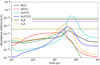 |
Fig. 4. Calculated fractional abundances of the six S-bearing species reported in this work as a function of time. Horizontal dotted lines correspond to observed values in TMC-1 adopting a column density of H2 of 1022 cm−2 (Cernicharo & Guélin 1987). |
The radical NCS is formed in the chemical model through the reactions CN + SO and N + HCS. The kinetics and product distribution of these reactions is, however, largely unconstrained. This uncertainty also affects the chemical network involving the family of CHNS isomers, for which the chemical model underestimates the column densities (see Table 1). In the chemical models of dark clouds performed by Adande et al. (2010) and Vidal et al. (2017), the main formation pathways to these molecules involve grain surface reactions, which are not included in our chemical network.
The formation of the other five molecules reported in this work, which are S-bearing carbon chains and thus can be represented by the formula HmCnS, occurs through two types of chemical routes. The first one involves neutral-neutral reactions. Along this pathway, HCCS is formed by the reactions C+H2CS and OH+C3S, the reaction S+C2H3 yields H2CCS, while H2CCCS is mostly formed by the reaction S+CH2CCH. On the other hand, the carbon chain C4S is formed through the reactions S+C4H and C+HC3S, while C5S is produced in the reactions C4H+CS and S+C5H. It must be noted that the kinetics and product distribution of these reactions is very poorly known. Most of these reactions are assumed to proceed with capture rate coefficients by Vidal et al. (2017).
The second pathway consists of reactions involving cations, which ultimately lead to the ion HpCnS+, which dissociatively recombines with electrons to yield HmCnS, where typically p = m + 1. In this route, the ions H2CCS+, H3CCS+, H3CCCS+, HC4S+, and HC5S+ are the precursors of HCCS, H2CCS, H2CCCS, C4S, and C5S, respectively. The abovementioned ions are in turn formed through reactions between atomic S with hydrocarbon ions and S+ with neutral hydrocarbons. In the same line of the reactions discussed above, there are large uncertainties regarding these reactions, for which rate coefficients and product distributions are taken from Vidal et al. (2017). The chemical network is probably incomplete in that it misses important reactions involving S and S+. Moreover, reactions on grain surfaces, which are considered by Vidal et al. (2017) but are not taken into account here, could play an important role.
4. Conclusions
In this work, we present the detection of five new sulfur-bearing molecules in TMC-1: NCS, HCCS, H2CCS, H2CCCS, and C4S. In addition, the species C5S previously found only towards carbon-rich circumstellar envelopes is also detected in a cold dark cloud for the first time. Chemical models fail to reproduce the observed column densities which implies that the chemical networks are incomplete and that laboratory and theoretical work has to be performed in order to understand the chemistry of sulfur in cold prestellar cores.
Acknowledgments
The Spanish authors thank Ministerio de Ciencia e Innovación for funding support through projects AYA2016-75066-C2-1-P, PID2019-106235GB-I00 and PID2019-107115GB-C21/AEI/10.13039/501100011033, and grant RyC-2014-16277. We also thank ERC for funding through grant ERC-2013-Syg-610256-NANOCOSMOS.
References
- Adande, G. R., Halfen, D. T., Ziurys, L. M., et al. 2010, ApJ, 725, 561 [Google Scholar]
- Agúndez, M., & Wakelam, V. 2013, Chem. Rev., 113, 8710 [Google Scholar]
- Agúndez, M., Cernicharo, J., & Guélin, M. 2014, A&A, 570, A45 [NASA ADS] [CrossRef] [EDP Sciences] [Google Scholar]
- Agúndez, M., Cernicharo, J., & Guélin, M. 2015, A&A, 577, L5 [NASA ADS] [CrossRef] [EDP Sciences] [Google Scholar]
- Agúndez, M., Marcelino, N., Cernicharo, J., & Tafalla, M. 2018, A&A, 611, L1 [NASA ADS] [CrossRef] [EDP Sciences] [Google Scholar]
- Amano, Takayosi, & Takako, Amano 1991, J. Chem. Phys., 95, 2275 [Google Scholar]
- Bell, M. B., Avery, L. W., & Feldman, P. A. 1993, ApJ, 417, L37 [Google Scholar]
- Brown, R. D., Godfrey, P. D., Champion, R., & Woodruff, M. 1982, Aust. J. Chem., 35, 1747 [CrossRef] [Google Scholar]
- Brown, R. D., Dyall, K. G., Elmes, P. S., et al. 1988, J. Am. Chem. Soc., 110, 789 [Google Scholar]
- Bulut, N., Roncero, O., Aguado, A., et al. 2021, A&A, 646, A5 [NASA ADS] [CrossRef] [EDP Sciences] [Google Scholar]
- Cabezas, C., Endo, Y., Roueff, E., et al. 2021, A&A, 646, L1 [NASA ADS] [CrossRef] [EDP Sciences] [Google Scholar]
- Cernicharo, J. 1985, Internal IRAM report (Granada: IRAM) [Google Scholar]
- Cernicharo, J. 2012, EAS Publ. Ser., 2012, 251, https://nanocosmos.iff.csic.es/?page_id=1619 [Google Scholar]
- Cernicharo, J., & Guélin, M. 1987, A&A, 176, 299 [Google Scholar]
- Cernicharo, J., Guélin, M., Hein, H., & Kahane, C. 1987, A&A, 181, L9 [Google Scholar]
- Cernicharo, J., Tercero, B., Fuente, A., et al. 2013, ApJ, 771, L10 [Google Scholar]
- Cernicharo, J., Cabezas, C., Pardo, J. R., et al. 2019, A&A, 630, L2 [NASA ADS] [CrossRef] [EDP Sciences] [Google Scholar]
- Cernicharo, J., Marcelino, N., Pardo, J. R., et al. 2020a, A&A, 641, L9 [NASA ADS] [CrossRef] [EDP Sciences] [Google Scholar]
- Cernicharo, J., Marcelino, N., Agúndez, M., et al. 2020b, A&A, 642, L8 [NASA ADS] [CrossRef] [EDP Sciences] [Google Scholar]
- Cernicharo, J., Marcelino, N., Agúndez, M., et al. 2020c, A&A, 642, L17 [NASA ADS] [CrossRef] [EDP Sciences] [Google Scholar]
- Cernicharo, J., Cabezas, C., Endo, Y., et al. 2021a, A&A, 646, L3 [EDP Sciences] [Google Scholar]
- Cernicharo, J., Cabezas, C., Bailleux, S., et al. 2021b, A&A, 646, L7 [NASA ADS] [CrossRef] [EDP Sciences] [Google Scholar]
- Cernicharo, J., Cabezas, C., Agúndez, M., et al. 2021c, A&A, 647, L3 [EDP Sciences] [Google Scholar]
- Crabtree, K. N., Martin-Drumel, M.-A., Brown, G. G., et al. 2016, J. Chem. Phys., 144 [Google Scholar]
- Dunning, T. H. 1989, J. Chem. Phys., 90, 1007 [Google Scholar]
- Endo, Y., Kohguchi, H., & Ohshima, Y. 1994, Faraday Discuss., 97, 341 [Google Scholar]
- Fossé, D., Cernicharo, J., Gerin, M., & Cox, P. 2001, ApJ, 552, 168 [Google Scholar]
- Frerking, M. A., Linke, R. A., & Thaddeus, P. 1979, ApJ, 234, L143 [NASA ADS] [CrossRef] [Google Scholar]
- Georgiou, K., Kroto, H. W., & Landsberg, B. M. 1979, J. Mol. Spectrosc., 77, 365 [NASA ADS] [CrossRef] [Google Scholar]
- Gordon, V. D., McCarthy, M. C., Apponi, A. J., & Thaddeus, P. 2001, ApJS, 134, 311 [NASA ADS] [CrossRef] [Google Scholar]
- Kaifu, N., Ohishi, M., Kawaguchi, K., et al. 2004, PASJ, 56, 69 [Google Scholar]
- Halfen, D. T., Ziurys, L. M., Brünken, S., et al. 2009, ApJ, 702, L124 [NASA ADS] [CrossRef] [Google Scholar]
- Hirahara, Y., Ohshima, Y., & Endo, Y. 1993, ApJ, 408, L113 [NASA ADS] [CrossRef] [Google Scholar]
- Hirahara, Y., Ohshima, Y., & Endo, Y. 1994, J. Chem. Phys., 101, 7342 [Google Scholar]
- Kim, E., Habara, H., & Yamamoto, S. 2002, J. Mol. Spectrosc., 212, 83 [CrossRef] [Google Scholar]
- Laas, J. C., & Caselli, P. 2019, A&A, 624, A108 [CrossRef] [EDP Sciences] [Google Scholar]
- Lee, S. 1997, Chem. Phys. Lett., 268, 69 [NASA ADS] [CrossRef] [Google Scholar]
- Lee, K. L., Martin-Drumel, M.-A., Lattanzi, V., et al. 2019, Mol. Phys., 117, 1381 [NASA ADS] [CrossRef] [Google Scholar]
- Lique, F., Cernicharo, J., & Cox, P. 2006, ApJ, 653, 1342 [NASA ADS] [CrossRef] [Google Scholar]
- Lique, F., Spielfield, A., Dubernet, M. L., & Feautrier, N. 2005, J. Chem. Phys., 123, 4316 [Google Scholar]
- Loison, J.-C., Agúndez, M., Marcelino, N., et al. 2016, MNRAS, 456, 4101 [Google Scholar]
- Maeda, A., Habara, H., & Amano, T. 2007, Mol. Phys., 105, 477 [NASA ADS] [CrossRef] [Google Scholar]
- Marcelino, N., Cernicharo, J., Agúndez, M., et al. 2007, ApJ, 665, L127 [Google Scholar]
- Marcelino, N., Agúndez, M., Cernicharo, J., et al. 2018, A&A, 612, L10 [NASA ADS] [CrossRef] [EDP Sciences] [Google Scholar]
- Marcelino, N., Agúndez, M., Tercero, B., et al. 2020, A&A, 643, L6 [NASA ADS] [CrossRef] [EDP Sciences] [Google Scholar]
- McCarthy, M. C., Coosky, A. L., Mohamed, S., et al. 2003, ApJS, 144, 287 [Google Scholar]
- McCarthy, M. C., Thaddeus, P., Wilke, J., et al. 2009, J. Chem. Phys., 130 [Google Scholar]
- McElroy, D., Walsh, C., Markwick, A. J., et al. 2013, A&A, 550, A36 [NASA ADS] [CrossRef] [EDP Sciences] [Google Scholar]
- McGuire, B. A., Martin-Drumel, M. A., Thorwirth, S., et al. 2016, Phys. Chem. Chem. Phys., 18, 22693 [Google Scholar]
- McGuire, B. A., Shingledecker, C. N., Willis, E. R., et al. 2019, ApJ, 883, 201 [Google Scholar]
- McNaughton, D., Robertson, E. G., & Hathlerly, L. D. 1996, J. Mol. Spectrosc., 175, 377 [Google Scholar]
- Müller, H. S. P., Schlöder, F., Stutzki, J., & Winnewisser, G. 2005, J. Mol. Struct., 742, 215 [Google Scholar]
- Pardo, J. R., Cernicharo, J., & Serabyn, E. 2001, IEEE Trans. Antennas Propag., 49, 12 [Google Scholar]
- Pascoli, G., & Lavendy, H. 1998, Int. Jour. Mass. Spectr., 181, 11 [Google Scholar]
- Petrie, S. 1996, MNRAS, 281, 666 [NASA ADS] [Google Scholar]
- Pickett, H. M., Poynter, R. L., Cohen, E. A., et al. 1998, J. Quant. Spectrosc. Radiat. Transfer, 60, 883 [Google Scholar]
- Puzzarini, C. 2008, Chem. Phys., 346, 45 [Google Scholar]
- Saito, S., Kawaguchi, K., Yamamoto, S., et al. 1987, ApJ, 317, L115 [Google Scholar]
- Tercero, F., López-Pérez, J. A., Gallego, J. D., et al. 2021, A&A, 645, A37 [EDP Sciences] [Google Scholar]
- Vastel, C., Quénard, D., Le Gal, R., et al. 2018, MNRAS, 478, 5514 [Google Scholar]
- Vidal, T. H. G., Loison, J.-C., Jaziri, A. Y., et al. 2017, MNRAS, 469, 435 [Google Scholar]
- Wakelam, V., Loison, J.-C., Herbst, E., et al. 2015, ApJS, 217, 20 [Google Scholar]
- Wierzejewska, M., & Moc, J. 2003, J. Phys. Chem. A, 107, 11209 [Google Scholar]
- Winnewiser, M., & Schäfer, E. 1980, Z. Naturforsch, 35a, 483 [Google Scholar]
- Yamamoto, S., Saito, S., Kawaguchi, K., et al. 1987, ApJ, 317, L119 [Google Scholar]
Appendix A: Column density and rotational temperature determination
In determining the column density of the molecules discovered and analysed in this work, we adopted a source of uniform brightness and 40″ radius (Fossé et al. 2001). We also adopted a full linewidth at half power intensity of 0.6 km s−1, which represents a good average value to the linewidth of all observed lines in this work.
For the species with more than one line observed, we performed rotation diagrams to derive the corresponding rotational temperatures and column densities. However, for species for which we observed less than three transitions, we adopted the same source parameters and a rotational temperature of 10 K. In some cases we adopted the rotational temperature derived for a similar species. The different derived and/or adopted rotational temperatures for each species are given in Table 1 along with the derived column densities. For CS, HCS+, CCS, and C3S, the column densities are taken from Cernicharo et al. (2021a). We note that the column density of CS, as its J = 1–0 line has a significant optical depth, was derived from that of C34S adopting the 32S/34S abundance ratio determined from C3S and C334S (24 ± 3) (Cernicharo et al. 2021a). A similar result is obtained from 13C34S adopting a 12C/13C abundance ratio of 90 (Cernicharo et al. 2020c). For all other molecules studied in this work, the lines are optically thin.
The error in getting column densities from the observed parameters of a single line and the assumed rotational temperature has been discussed in detail by Cernicharo et al. (2021a). In fact, the main source of uncertainty when the energy of the levels involved in the transition is ≤TK is not the assumed rotational temperature itself, but the assumption of it being uniform for all rotational levels (Cernicharo et al. 2021a). For example, changing the rotational temperature from 5 to 10 K for transitions J = 1–0 or J = 2–1 has a very modest effect on the column density (see, e.g. Cernicharo et al. 2021a and Cabezas et al. 2021). This is due to the fact that intensities are proportional to the rotational temperature Tr, but the partition function is inversely proportional to Tr for linear molecules. This also applies to asymmetric species with a large rotational constant A, which is much larger than Tr (H2CCS and H2CCCS, for example).
As a final check on the derived column densities, we also used the synthetic spectrum resulting from the best fit model to all lines of a molecule computed with the MADEX code (Cernicharo 2012). The final parameters derived this way should be very similar to those that could be derived from a standard rotation diagram. Nevertheless, this model fit allows one to compare the synthetic line profiles with observed ones, which is particularly interesting when the rotational transitions exhibit a hyperfine structure as is the case here for HCS, HSC, and HSCN, and to a lesser extent for HNCS.
Appendix B: Stacking spectra
For C4S and C5S, we observed several individual lines and their detection is solid. In order to provide additional support for it, we stacked the data following the procedure used recently to detect CH3CH2CCH in TMC-1 (Cernicharo et al. 2021c). The data were normalised to the expected intensity of each transition computed under local thermodynamic equilibrium (LTE) for the rotational temperature derived from the analysis of the individual lines. Finally, all the data were multiplied by the expected intensity of the strongest transition among the selected ones. The lines are optically thin, hence, the intensity of all lines scale in the same way with the assumed column density. Each individual spectra is weighted as 1/ , where σN now accounts for the normalisation intensity factor.
In order to strengthen the detection of C4S, we grouped the observed lines into two different sets. The first one, with six lines, corresponds to the strongest transitions for Tr = 7 K (J = N + 1 transitions). A second group consists of thirteen lines corresponding to the weak J = N and J = N − 1 transitions, which are 2–3 times weaker than those of the first group for the derived rotational temperature and, therefore, are below the 3σ detection limit for individual lines (∼0.9–1.5 mK) in the observed frequency range. We again normalised all spectra to the predicted intensity of the strongest line (NJ = 1011 − 910) and averaged all the data in each set using the root mean square noise of each normalised spectrum as a weighting factor. We verified that none of these lines are contaminated by an unknown feature or from a transition of a known molecular species (it could appear centred on the local standard of rest velocity of the cloud). In all individual spectra, the emission from other features outside the expected velocity range was removed by blanking the channels (for example the line of C3O in the NJ = 1213 − 1112 spectrum; see Fig. B.1). Negative features due to the frequency switching folding were also eliminated before stacking the data. As quoted above, four of the six strongest lines are clearly detected (see Fig. B.1), and the other two do not show any significant emission at the expected velocity (their intensities are predicted to be 1.5–2 times weaker than the strongest transition). The stacked spectrum clearly shows a spectral feature at the expected velocity with a signal-to-noise ratio of ≃7, as shown in panel b of Fig. B.1. For the group of thirteen weak lines, the resulting stacked spectrum is shown in panel c of the same figure. A line at 4σ is detected. Hence, the detection of the C4S radical is robust.
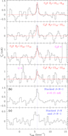 |
Fig. B.1. Four upper panels: individual lines of C4S with J = N + 1 detected in our survey. Two bottom panels: spectrum obtained after stacking all lines of C4S with J = N + 1 (panel b) and the resulting spectrum after stacking the twelve weak lines with J = N and J = N − 1 (panel c). The abscissa corresponds to the velocity with respect to the local standard of rest. The dashed blue line corresponds to vLSR = 5.83 km s−1. The ordinate is the antenna temperature in milliKelvin. The red line in the four upper panels corresponds to the synthetic spectrum for each transition computed with Tr = 7 K and N(C4S) = 3.8 × 1010 cm−2. |
For C5S, the detection of five individual lines (see Fig. B.2) provides solid evidence on the detection of this species in TMC-1. The observed transitions have upper energy levels between 13 and 20 K. Three additional transitions above 40 GHz have intensities too low to be detected with the present sensitivity. Nevertheless, the stacked spectrum of all transitions results on a line at 8σ. Hence, we conclude that the detection of these two S-bearing carbon chains in TMC-1 is solid and convincing.
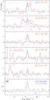 |
Fig. B.2. Detected lines of C5S within the observed frequency range. The abscissa corresponds to the velocity with respect to the local standard of rest. The ordinate is the antenna temperature corrected for atmospheric and telescope losses in milliKelvin. Spectral resolution is 38.15 kHz. The dashed blue line corresponds to vLSR = 5.83 km s−1. The red line represents the synthetic spectrum for each line computed for Tr = 7 K and N(C5S) = 5 × 1010 cm−2. Panel b: stacked spectrum of all rotational transitions of C5S in our survey from Ju = 17 to 27. |
Appendix C: Abundances of related sulfur-bearing species
C.1. HCS and HSC
HCS and HSC were discovered by Agúndez et al. (2018) towards L483. Here, we present the first detection of these species in TMC-1. The observed lines are shown in Figs. C.1 and C.2, respectively. Assuming a rotational temperature of 5 K, we derived N(HCS) = (5.5 ± 0.5) × 1012 cm−2 and N(HSC) = (1.3 ± 0.1) × 1011 cm−2. The column densities increase by ∼20% if a rotational temperature of 10 K is assumed. The derived abundance ratio X(HCS)/X(HSC) is 42 ± 7, which is very similar to the value derived by Agúndez et al. (2018) towards L483. However, we derived an abundance ratio H2CS/HCS of ∼9, while in L483 this ratio is ∼1. Our purely gas-phase chemical model results in a H2CS/HCS ratio of ∼200 (see Table 1) that is too high compared with the values observed in TMC-1 and L483, although the chemical model of Vidal et al. (2017), which includes grain-surface reactions, predicts a H2CS/HCS ratio close to the value observed in TMC-1. In the case of HCS and HSC, we could speculate with a common precursor, HCSH+. However, as discussed by Agúndez et al. (2018), the most stable isomer of this cation is H2CS+ and the formation of HSC from its dissociative recombination requires a substantial rearrangement of the molecular structure. If, as suggested by those authors that the CH3S+ cation is the common precursor of H2CS and HCS, additional reactions are needed to explain the different H2CS/HCS abundance ratio found towards TMC-1 and L483.
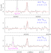 |
Fig. C.1. Observed lines of HCS within the observed frequency range. The abscissa corresponds to the rest frequency assuming a velocity with respect to the local standard of rest of 5.83 km s−1. The ordinate is the antenna temperature corrected for atmospheric and telescope losses in milliKelvin. Spectral resolution is 38.15 kHz. The red line shows the synthetic spectrum for Tr = 5 K and N = (5.50 ± 0.50) × 1012. |
C.2. SO, H2CS, and OCS
We note that SO and NS do not have strong transitions in the 31–50 GHz domain; SO has one transition in this domain, the 32 − 22, but its upper energy level is 21.1 K and we observed a weak emission feature at the correct frequency (see Table D.1). This line has peculiar excitation conditions as it turns out to be in absorption in front of the cosmic microwave background for low volume densities and in emission for the typical densities of TMC-1. Lique et al. (2006) studied SO in detail in this cloud and they derived an abundance of ∼10−8. Using the collisional rates of Lique et al. (2005), we derived a brightness temperature for the 32–22 transition of SO of −21, −17, 1.8, and 38 mK for n(H2) = 104, 4 × 10⁴, 6 × 10⁴, and 105 cm−3, respectively. The predicted intensity has a direct dependency on the column density, but the turnover between absorption and emission essentially depends on the volume density. From the observed parameters for this line (see Table D.1) and the abundance derived by Lique et al. (2006), we estimate a volume density for the core of TMC-1 of 4–6 × 104 cm−3, which is in good agreement with previous studies (see, e.g. Fossé et al. 2001 and Lique et al. 2006). Assuming the H2 column density derived by Cernicharo & Guélin (1987), the column density of SO is ∼1014 cm−2.
In our 7 mm line survey, H2CS only has one transition. Both, the main and the 34 isotopologues have been detected. Line parameters are given in Table D.1. The column density for this species was derived assuming a rotational temperature of 10 K (Cernicharo et al. 2021a).
It is important note that OCS has two transitions in the 31–50 GHz domain. Line parameters are given in Table D.1.
C.3. HNCS, HSCN, HCNS, and HSNC
We note that HNCS and HSCN have been previously detected in the interstellar medium (Frerking et al. 1979; Halfen et al. 2009). They are the sulfur equivalent of the well known molecules HNCO and HOCN; HNCS is the most stable among the possible CHNS isomers, with HSCN, HCSN, and HSNC being 3200, 17 300, and 18 100 K above HNCS, respectively (Wierzejewska & Moc 2003).
Adande et al. (2010) have already observed HSCN and HNCS in TMC-1. We observed the 30, 3–20, 2 and 40, 4–30, 3 transitions of both species, with the corresponding fine structure components for HSCN. The observed lines are shown in Fig. C.3. By performing a model fitting through the synthetic spectrum, we conclude that a rotational temperature in the range of 5–8 K produces a good match, although the best agreement is found for Tr = 5 K (see Fig. C.3). We derived a column density of (3.8 ± 0.4) × 1011 cm−2, for HNCS and (5.8 ± 0.6) × 1011 cm−2, for HSCN. It seems that HSCN is slightly more abundant than HNCS, despite being less stable, with an abundance ratio of HSCN/HNCS = 1.5 ± 0.3. The column densities of HNCS and HSCN derived by Adande et al. (2010) are somewhat lower than those derived here, although the ratio HSCN/HNCS derived by these authors is also around one.
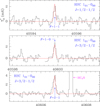 |
Fig. C.2. Observed lines of HSC within the observed frequency range. The abscissa corresponds to the rest frequency assuming a velocity with respect to the local standard of rest of 5.83 km s−1. The ordinate is the antenna temperature corrected for atmospheric and telescope losses in milliKelvin. Spectral resolution is 38.15 kHz. The red line shows the synthetic spectrum for Tr = 5 K and N = (5.50 ± 0.50) × 1012. |
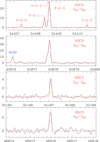 |
Fig. C.3. Observed lines of HSCN and HNCS within the observed frequency range. The abscissa corresponds to the rest frequency assuming a velocity with respect to the local standard of rest of 5.83 km s−1. The ordinate is the antenna temperature corrected for atmospheric and telescope losses in milliKelvin. Spectral resolution is 38.15 kHz. The red line shows the synthetic spectrum for Tr = 5 K and N = (5.80 ± 0.60) × 1011 cm−2 for HSCN, and N = (3.80 ± 0.40) × 1011 cm−2 for HNCS. |
The oxygen analogues HNCO and HOCN have a very different abundance ratio in TMC-1, where HNCO/HOCN ∼130 (Cernicharo et al. 2020c). The same behaviour is observed in warm molecular clouds, where HNCS and HSCN have comparable abundances, while HNCO is two orders of magnitude more abundant than HOCN (Adande et al. 2010). These authors argue that HSCN and HCSN could arise from a common precursor, HSCNH+, while HNCO may arise mostly from H2NCO+. However, the uncertainties in the chemical networks regarding the chemistry of CHNO and CHNS isomers are still large. It is interesting to note that while in L483, the abundance ratio HNCO/NCO is ∼5 (Marcelino et al. 2018), in TMC-1 the HNCS/NCS ratio is ∼0.5. This fact strengthens the different behaviour of the CHNO and CHNS systems in interstellar clouds.
We also searched for the two isomers HCNS and HSNC (thio and isothio fulminic acid, respectively) for which laboratory spectroscopy is available (McGuire et al. 2016). We derived a 3σ upper limit to their column density of 6 × 1010 cm−2, and 2 × 1010 cm−2, respectively.
C.4. HCCSH, HCCCSH, and HSCS+
We note that HCCSH is a metastable isomer, with an energy of 6770 K above the most stable isomer H2CCS (Lee et al. 2019). It has been searched for towards several sources (McGuire et al. 2019), but only upper limits have been obtained for its abundance. In TMC-1, McGuire et al. (2019) derived a 1σ upper limit to its column density of ≤2.9 × 1013 cm−2. In our Q-band data, we have searched for the lines of this species. Assuming a rotational temperature of 7 K, we derived a 3σ upper limit of N ≤ 9 × 1012 cm−2. The rather poor upper limit is due to its low μa dipole moment μa = 0.13 D (Lee et al. 2019). The b component of the dipole moment is larger, but b-type transitions for this species are outside the frequency range of our survey and they involve energy levels that will be unpopulated under the physical conditions of TMC-1.
We also searched for HCCCSH, an isomer of H2CCCS, which is predicted to lie around 1000 K above it (Brown et al. 1982; Crabtree et al. 2016), but only a 3σ upper limit to its column density of 2.4 × 1011 cm−2, was obtained (see Table 1). It is interesting to note that in TMC-1, the abundance ratio HCCCHO/H2CCCO is well above one (Loison et al. 2016; Cernicharo et al. 2020c), while the HCCCSH/H2CCCS ratio is found to be below one.
Finally, we have also searched for HSCS+ (McCarthy et al. 2009), the protonated form of carbon disulfide. Due to its low dipole moment (McCarthy et al. 2009), the derived 3σ upper limit for its column density is ≤3.0 × 1012 cm−2 (average result from the four lines in our survey).
Appendix D: Line parameters
Line parameters for all observed transitions were derived by fitting a Gaussian line profile to them. A velocity range of ±20 km s−1, around each feature was considered for the fit after a polynomial baseline was removed. The derived line parameters are given in Table D.1.
Observed line parameters for sulfur-bearing species in TMC-1.
Appendix E: New reactions included
Reactions involving S-bearing species not included in either the chemical network UMIST RATE12 or that of Vidal et al. (2017).
All Tables
Reactions involving S-bearing species not included in either the chemical network UMIST RATE12 or that of Vidal et al. (2017).
All Figures
|
Fig. 1. Observed lines of HCCS (panel a) and NCS (panels b and c) towards TMC-1. The abscissa corresponds to the rest frequency assuming a local standard of rest velocity of the source of 5.83 km s−1 (see text). Blanked channels correspond to negative features produced in the frequency switching data folding. The ordinate is the antenna temperature corrected for atmospheric and telescope losses in milliKelvin. Spectral resolution is 38.15 kHz. The red lines show the synthetic spectrum of HCCS and NCS for a rotational temperature of 5 K, a linewidth of 0.6 km s−1, and a column density of 6.8 × 1011 cm−2 and 7.8 × 1011 cm−2, respectively. |
| In the text | |
|
Fig. 2. Observed transitions of H2CCS towards TMC-1. The abscissa corresponds to the velocity in km s−1 of the source with respect to the local standard of rest. Line parameters are given in Table D.1. The ordinate is the antenna temperature corrected for atmospheric and telescope losses in milliKelvin. Blanked channels correspond to negative features produced by the folding of the frequency switching observations. The vertical blue dashed line indicates the vLSR of the cloud (5.83 km s−1). The red line spectra correspond to the synthetic model spectrum for each line adopting Tr = 7 K, N(o-H2CCS) = 6.0 × 1011 cm−2, and N(p-H2CCS) = 1.8 × 1011 cm−2 (see text). |
| In the text | |
|
Fig. 3. Selected transitions of H2CCCS towards TMC-1. The abscissa corresponds to the velocity in km s−1 of the source with respect to the local standard of rest. Line parameters are given in Table D.1. The ordinate is the antenna temperature corrected for atmospheric and telescope losses in milliKelvin. Blanked channels correspond to negative features produced by the folding of the frequency switching observations. The vertical blue dashed line indicates the vLSR of the cloud (5.83 km s−1). The red line spectra correspond to the synthetic model of the emission obtained for Tr = 10 K, N(o-H2CCS) = 3.0 × 1011 cm−2, and N(p-H2CCS) = 6.5 × 1010 cm−2. |
| In the text | |
|
Fig. 4. Calculated fractional abundances of the six S-bearing species reported in this work as a function of time. Horizontal dotted lines correspond to observed values in TMC-1 adopting a column density of H2 of 1022 cm−2 (Cernicharo & Guélin 1987). |
| In the text | |
|
Fig. B.1. Four upper panels: individual lines of C4S with J = N + 1 detected in our survey. Two bottom panels: spectrum obtained after stacking all lines of C4S with J = N + 1 (panel b) and the resulting spectrum after stacking the twelve weak lines with J = N and J = N − 1 (panel c). The abscissa corresponds to the velocity with respect to the local standard of rest. The dashed blue line corresponds to vLSR = 5.83 km s−1. The ordinate is the antenna temperature in milliKelvin. The red line in the four upper panels corresponds to the synthetic spectrum for each transition computed with Tr = 7 K and N(C4S) = 3.8 × 1010 cm−2. |
| In the text | |
|
Fig. B.2. Detected lines of C5S within the observed frequency range. The abscissa corresponds to the velocity with respect to the local standard of rest. The ordinate is the antenna temperature corrected for atmospheric and telescope losses in milliKelvin. Spectral resolution is 38.15 kHz. The dashed blue line corresponds to vLSR = 5.83 km s−1. The red line represents the synthetic spectrum for each line computed for Tr = 7 K and N(C5S) = 5 × 1010 cm−2. Panel b: stacked spectrum of all rotational transitions of C5S in our survey from Ju = 17 to 27. |
| In the text | |
|
Fig. C.1. Observed lines of HCS within the observed frequency range. The abscissa corresponds to the rest frequency assuming a velocity with respect to the local standard of rest of 5.83 km s−1. The ordinate is the antenna temperature corrected for atmospheric and telescope losses in milliKelvin. Spectral resolution is 38.15 kHz. The red line shows the synthetic spectrum for Tr = 5 K and N = (5.50 ± 0.50) × 1012. |
| In the text | |
|
Fig. C.2. Observed lines of HSC within the observed frequency range. The abscissa corresponds to the rest frequency assuming a velocity with respect to the local standard of rest of 5.83 km s−1. The ordinate is the antenna temperature corrected for atmospheric and telescope losses in milliKelvin. Spectral resolution is 38.15 kHz. The red line shows the synthetic spectrum for Tr = 5 K and N = (5.50 ± 0.50) × 1012. |
| In the text | |
|
Fig. C.3. Observed lines of HSCN and HNCS within the observed frequency range. The abscissa corresponds to the rest frequency assuming a velocity with respect to the local standard of rest of 5.83 km s−1. The ordinate is the antenna temperature corrected for atmospheric and telescope losses in milliKelvin. Spectral resolution is 38.15 kHz. The red line shows the synthetic spectrum for Tr = 5 K and N = (5.80 ± 0.60) × 1011 cm−2 for HSCN, and N = (3.80 ± 0.40) × 1011 cm−2 for HNCS. |
| In the text | |
Current usage metrics show cumulative count of Article Views (full-text article views including HTML views, PDF and ePub downloads, according to the available data) and Abstracts Views on Vision4Press platform.
Data correspond to usage on the plateform after 2015. The current usage metrics is available 48-96 hours after online publication and is updated daily on week days.
Initial download of the metrics may take a while.