| Issue |
A&A
Volume 688, August 2024
|
|
|---|---|---|
| Article Number | L13 | |
| Number of page(s) | 5 | |
| Section | Letters to the Editor | |
| DOI | https://doi.org/10.1051/0004-6361/202451256 | |
| Published online | 07 August 2024 | |
Letter to the Editor
More sulphur in TMC-1: Discovery of the NC3S and HC3S radicals with the QUIJOTE line survey⋆
1
Dept. de Astrofísica Molecular, Instituto de Física Fundamental (IFF-CSIC), C/ Serrano 121, 28006 Madrid, Spain
e-mail: This email address is being protected from spambots. You need JavaScript enabled to view it.
2
Observatorio Astronómico Nacional (OAN, IGN), C/ Alfonso XII, 3, 28014 Madrid, Spain
3
Observatorio de Yebes (IGN), Cerro de la Palera s/n, 19141 Yebes, Guadalajara, Spain
Received:
25
June
2024
Accepted:
5
July
2024
Abstract
We present the detection of the free radicals NC3S and HC3S towards TMC-1 with the QUIJOTE line survey. The derived column densities are (1.4 ± 0.2)×1011 for NC3S and (1.5 ± 0.2)×1011 for HC3S. We searched for NCCS, but only three transitions are within the domain of our QUIJOTE line survey and the observed lines are marginally detected at the 3σ level, providing an upper limit to its column density of ≤6 × 1010 cm−2. We also unsuccessfully searched for longer species of the NCnS (n ≥ 4) and HCnS (n ≥ 5) families in our TMC-1 data. A chemical model based on a reduced set of reactions involving HC3S and NC3S predicts abundances that are 10–100 times below the observed values. These calculations indicate that the most efficient reactions of formation of HC3S and NC3S in the model are S + C3H2 and N + HC3S, respectively, while both radicals are very efficiently destroyed through reactions with neutral atoms.
Key words: astrochemistry / line: identification / molecular data / ISM: molecules / ISM: individual objects: TMC-1
Based on observations with the Yebes 40 m telescope (projects 19A003, 20A014, 20D023, 21A011, 21D005, and 23A024). The 40 m radio telescope at Yebes Observatory is operated by the Spanish Geographic Institute (IGN; Ministerio de Transportes y Movilidad Sostenible).
© The Authors 2024
 Open Access article, published by EDP Sciences, under the terms of the Creative Commons Attribution License (https://creativecommons.org/licenses/by/4.0), which permits unrestricted use, distribution, and reproduction in any medium, provided the original work is properly cited.
This article is published in open access under the Subscribe to Open model. This email address is being protected from spambots. You need JavaScript enabled to view it. to support open access publication.
1. Introduction
A significant number of S-bearing species have been detected in the starless core TMC-1. In particular, the species CS, CCS, and CCCS are among the most abundant molecules in cold dark clouds (Saito et al. 1987; Yamamoto et al. 1987; Kaifu et al. 1987) and in the circumstellar envelopes of carbon-rich evolved stars (Cernicharo et al. 1987). The abundance and variety of sulphur-bearing species detected to date in cold clouds is hampered, to a large extent, by the significant depletion of sulphur in the cloud (Vidal et al. 2017; Fuente et al. 2019, 2023; Navarro-Almaida et al. 2020 and references therein) and by the lack of sensitive line surveys that allow the detection of low-abundance, or high-abundance but low-dipole moment, S-bearing molecules.
In the last four years, our knowledge of the chemical composition of TMC-1 regarding sulphur has experienced an enormous advancement with the discovery of 14 new sulphur-bearing molecules thanks to the ultra-sensitive QUIJOTE1 line survey (Cernicharo et al. 2021a). Neutral species such as C4S, C5S (previously detected only towards evolved stars), HCCS, H2CCS, H2CCCS, NCS, HSO, HCSCN, HCSCCH, HC4S, HCNS, and NCCHCS have been detected with QUIJOTE (Cernicharo et al. 2021b,c, 2024a; Fuentetaja et al. 2022; Marcelino et al. 2023; Cabezas et al. 2024). In addition, cations such as HCCS+ (Cabezas et al. 2022) and HC3S+ (Cernicharo et al. 2021d) have also been found in this cloud. Chemical models are being continuously improved and refined to shed light on the formation and destruction pathways of all these newly detected species.
The continuous sensitivity increase of the QUIJOTE line survey makes it well suited to detect additional heavier S-bearing species. In this context we present in this Letter the discovery, for the first time in space, of the radicals HC3S and NC3S. Only upper limits have been obtained for the column densities of longer members of the HCnS and NCnS families. The formation and destruction pathways of HC3S and NC3S are analysed with state-of-the-art chemical models. With the detection of HC3S and NC3S, QUIJOTE has provided the identification of 16 new S-bearing molecules in space.
2. Observations
The observational data used in this work are from QUIJOTE (Cernicharo et al. 2021a), a spectral line survey of TMC-1 in the Q band carried out with the Yebes 40 m telescope at the position αJ2000 = 4h41m41.9s and δJ2000 = +25° 41′27.0″, which corresponds to the cyanopolyyne peak in TMC-1. The receiver was built as part of the Nanocosmos project2 and consists of two cold high-electron mobility transistor amplifiers covering the 31.0–50.3 GHz band with horizontal and vertical polarizations. Receiver temperatures vary between 16 K at 32 GHz and 30 K at 50 GHz. The back ends are 2 × 8 × 2.5 GHz fast Fourier transform spectrometers with a spectral resolution of 38 kHz, providing the whole coverage of the Q band in both polarizations. A detailed description of the system is given by Tercero et al. (2021), and details on the QUIJOTE line survey observations have previously been provided (Cernicharo et al. 2021a, 2023a,b; Cernicharo et al. 2024a,b). The frequency switching method was used for all observations. The data analysis procedure has been described by Cernicharo et al. (2022). The total observing time on source is 1202 hours, and the measured sensitivity varies between 0.08 mK at 32 GHz and 0.2 mK at 49.5 GHz.
The main beam efficiency can be given across the Q band as ηeff = 0.797 exp[−(ν(GHz)/71.1)2]. The forward telescope efficiency is 0.95, and the beam size at half power intensity is 54.4″ and 36.4″ at 32.4 and 48.4 GHz, respectively. The absolute intensity calibration uncertainty is 10%, although the relative calibration between lines within the QUIJOTE survey is certainly better because all of them are observed simultaneously and have the same calibration uncertainties and systematic effects. The data were analysed with the GILDAS package3.
3. Results
Line identification in this work was performed using the MADEX code (Cernicharo 2012), in addition to the CDMS and JPL catalogues (Müller et al. 2005; Pickett et al. 1998). The intensity scale utilized in this study is the antenna temperature ( ). Consequently, the telescope parameters and source properties were used when modelling the emission of the different species to produce synthetic spectra on this temperature scale. In this work we assumed a velocity for the source relative to the local standard of rest of 5.83 km s−1 (Cernicharo et al. 2020). The source was assumed to be circular with a uniform brightness temperature and a radius of 40″ (Fossé et al. 2001). Line parameters for all observed transitions with the Yebes 40 m radio telescope were derived by fitting a Gaussian line profile to them using the GILDAS package. A velocity range of ±20 km s−1 around each feature was considered for the fit after a polynomial baseline was removed. Negative features produced in the folding of the frequency switching data were blanked before baseline removal. The observed line intensities were modelled using a local thermodynamical equilibrium hypothesis. The laboratory data used in this work are discussed in the following sections. We first discuss NC3S because its detection motivated the search for NCCS and other longer NCnS chains.
3.1. Discovery of NC3S
We have found a series of six harmonically related lines with half-integer quantum numbers from J = 23/2 − 21/2 to J = 33/2 − 31/2. The lines are shown in Fig. 1. The two first lines clearly show hyperfine structure, which suggests the presence of a nitrogen atom in the molecule. The other lines are also broader with respect to the standard lines from other species (Δv = 0.6 − 0.7 km s−1). We were able to fit the frequency centroids (see Table 1) with the standard relation for the frequencies of a linear molecule, finding an effective rotational constant, Beff, of 1438.9761 ± 0.0003 MHz and an effective distortion constant, Deff, of 47.6 ± 0.6 Hz. The standard deviation of the fit is 4.1 kHz. We verified that the lines cannot be produced by a species with a rotational constant half of the derived one (all lines with even Js would be missing in that case). The half-integer quantum numbers indicate that the carrier is a radical.
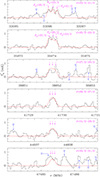 |
Fig. 1. Observed transitions of NC3S. Quantum numbers are indicated at the top right of each panel. The abscissa corresponds to the rest frequency. The ordinate is the antenna temperature, corrected for atmospheric and telescope losses, in millikelvins. Blank channels correspond to negative features produced when folding the frequency-switched data. The purple vertical arrows indicate the position of the three strongest hyperfine components for each transition, corresponding to Fu = Ju + 1, Ju, and Ju − 1. The red line shows the modelled spectra for NC3S with the physical parameters given in Sect. 3.1. |
Estimated line parameters for the observed lines of NC3S.
The lines do not appear in any of the line catalogues available to us. The recent discovery of HC5N+ with a rotational constant of 1336.6 MHz (Cernicharo et al. 2024b) pointed us towards the possibility of an isomer of this molecule. Accurate ab initio calculations, however, permitted us to discard all of them. A species recently detected in TMC-1 is HC4S (Fuentetaja et al. 2022), which has a rotational constant of 1435.3 MHz and a 2Π inverted ground electronic state (Hirahara et al. 1994). Hence, the carrier should be a molecule similar to HC4S but containing a nitrogen atom. Taking into account that NCS has already been detected in TMC-1 (Cernicharo et al. 2021b), we conclude that NC3S is a solid candidate to be the carrier of the observed lines. This species was not included in the MADEX code, nor in the CDMS or JPL catalogues. However, a quick search in the literature indicates that the molecule has been studied in the laboratory by McCarthy et al. (2003), together with other longer members of the NCnS family.
NC3S has an inverted 2Π ground electronic state, and the transitions observed in the laboratory by McCarthy et al. (2003) cover from J = 5/2 − 3/2 up to J = 17/2 − 15/2, which corresponds to frequencies up to 24.46 GHz. These data were fitted using SPFIT (Pickett 1991), and the molecule was implemented in the MADEX code to produce predictions in the frequency domain of QUIJOTE. The spin-orbit constant was fixed to the value given by McCarthy et al. (2003), ASO = −9.8209 THz. With such a high value for the spin-orbit constant, the energy levels of the 2Π1/2 ladder are above 470 K, and hence, no lines from this state are expected in TMC-1, where the kinetic temperature is 9 K (Agúndez et al. 2023). The derived rotational constant is B0 = 1439.18582 ± 0.00008 MHz, from which an effective rotational constant for the 2Π3/2 ladder can be derived from the relation Beff = B0(1 + B0/ASO). Using the molecular constants derived by McCarthy et al. (2003), we derive Beff(2Π3/2) = 1438.97492 ± 0.00008 MHz, which is nearly identical to that derived for our series of lines in TMC-1 (a difference of 1.2 kHz). The distortion constant of NC3S derived from the laboratory data is 45.8 ± 0.8 Hz, also in excellent agreement with that derived for our series of lines. Hence, we conclude that the carrier of our lines is, without any doubt, NC3S.
The lines observed in the laboratory for this species exhibit a prominent hyperfine structure introduced by the nitrogen nucleus. However, no Λ-doubling splitting was found. As an example, the three strongest components of the J = 17/2 − 15/2 transition at 24.6 GHz span 0.5 MHz. The frequency predictions indicate that the J = 23/2 − 21/2 and 25/2–23/2 lines observed in TMC-1 will show a considerable splitting, as observed in our lines (see Fig. 1). All the other transitions within the frequency range of our data are predicted to have a significant line broadening. We merged the astronomical frequencies with the laboratory values to try to improve the rotational constants of NC3S. However, such an improvement was marginal as the derived parameters are nearly the same as those of McCarthy et al. (2003).
To derive the column density of NC3S, we adopted a dipole moment of 3.0 D (McCarthy et al. 2003). We fitted the observed line profiles and intensities assuming a source of uniform brightness temperature. We obtain Trot = 5.5 ± 0.5 K and a column density of (1.4 ± 0.2) × 1011 cm−2. The source diameter that best fits the data is 70″. The observed line profiles are nicely reproduced by the modelled synthetic spectra shown in red in Fig. 1.
3.2. Search for NCCS and longer NCnS chains
Since NCS and NC3S are detected (Cernicharo et al. 2021b, and this work), it was worthwhile searching for NCCS in our data. Similarly to NC3S, the NCCS species was not included in the MADEX code, nor in the CDMS or JPL catalogues. However, the bent radical NCCS (X2A′) was studied via Fourier-transform microwave spectroscopy by Nakajima et al. (2003) up to 22.6 GHz, corresponding to the 404 − 303 transition. Only Ka = 0 transitions were observed in the laboratory. The observed frequencies were fitted using the SPFIT code (Pickett 1991) to produce predictions in the frequency domain of QUIJOTE. The A constant was fixed to 186.47 GHz; hence, the Ka = 1 lines are ∼9 K above the Ka = 0 ones and will have a considerable frequency uncertainty. The first Ka = 1 line in our data is the 616 − 515 with an upper energy level at 14.4 K. For an expected rotational temperature of 5–6 K, as found for another three or four atoms species, the expected intensities of the Ka = 1 lines will be a factor of five weaker than those of the Ka = 0 ones. Three transitions with Ka = 0 can be explored with our data (Nup = 6, 7, and 8). These lines show two fine components with J = N + 1/2 and J = N − 1/2, and an additional hyperfine splitting introduced by the nitrogen atom. The fine and hyperfine components of each rotational transition span 200 kHz. Unfortunately, some lines are blended, and the other lines are only detected at a marginal 3σ level. The dipole moment of NCCS has been calculated to be 2.49 D (McCarthy et al. 2003). Using this value, we derive a 3σ upper limit to the column density of this radical of ≤6 × 1010 cm−2.
Laboratory data for NC4S, NC5S, NC6S, and NC7S are also available from the study of McCarthy et al. (2003). We implemented these molecules in MADEX and searched for them in our data. However, none of their lines were detected. The 3σ upper limits to their column densities are in the range (8–10) × 1010 cm−2.
3.3. Discovery of HC3S
HCCS and HC4S have been detected in TMC-1 (Cernicharo et al. 2021b; Fuentetaja et al. 2022); hence, we could expect HC3S to also be present in the cloud. Rotational spectroscopy for HC3S is available from the studies of McCarthy et al. (1994) and Hirahara et al. (1994). The dipole moment was estimated to be 1.76 D through ab initio calculations (McCarthy et al. 1994). Frequency predictions for this species are available in the CDMS catalogue; hence, we implemented them into the MADEX code to obtain frequency predictions for the rotational transitions inside the frequency coverage of QUIJOTE. Three of these transitions – with Jup = 13/2, 15/2, and 17/2 – are in our data.
The lines of the 2Π1/2 ladder of HC3S exhibit Λ-doubling splitting that produces two components, e and f, for each rotational transition. In addition, each of these e and f components is further split into two hyperfine components due to the spin 1/2 of the unpaired electron. Hence, the three rotational transitions of HC3S that can be observed in our data will produce a total of 12 well-resolved features. Figure 2 shows the observed lines. Although the e component of the J = 13/2 − 11/2 transition is partially blended with C5H5CN, the two hyperfine components can be seen and adjusted. All the other lines are well detected. However, due to the partial blending between the Fu = Ju + 1/2 and Fu = Ju − 1/2 hyperfine components, a fixed linewidth of 0.7 km s−1 was adopted for all the lines. We conclude that we have detected enough individual lines of HC3S in TMC-1 to confidently claim its first detection in space. The derived line parameters are given in Table 2.
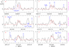 |
Fig. 2. Observed transitions of HC3S. Quantum numbers are indicated at the right side of each row. The abscissa corresponds to the rest frequency. The ordinate is the antenna temperature, corrected for atmospheric and telescope losses, in millikelvins. Blank channels correspond to negative features produced when folding the frequency-switched data. The Λ-doubling components e and f for each J are shown in the left and right panels, respectively. In addition, the two hyperfine components of each e and f rotational transition are resolved in our data and appear clearly detected. They correspond to Fu = Ju + 1/2 and Ju − 1/2. The red line shows the modelled spectra for HC3S with the physical parameters given in Sect. 3.3. |
Estimated line parameters for the observed lines of HC3S.
We adopted the same physical parameters for the cloud as for NC3S and derive a rotational temperature of 6.0 ± 0.5 K and a column density of (1.5 ± 0.2)×1011 cm−2, which is roughly a factor of two below the upper limit derived by Cernicharo et al. (2021b). The HCS and HCCS column densities have been derived to be (5.5 ± 0.5)×1012 and (6.8 ± 0.6)×1011 cm−2, respectively (Cernicharo et al. 2021b). HC4S was recently discovered towards TMC-1 by Fuentetaja et al. (2022) with an estimated column density of (9.5 ± 0.8)×1010 cm−2. Consequently, we derive the following abundance ratios: HCS/HCCS = 8.1 ± 1.6, HCCS/HC3S = 4.5 ± 1.0, and HC3S/HC4S = 1.6 ± 0.3. It seems, hence, that longer members of the HCnS family could be present in significant abundances in TMC-1.
HC5S was observed in the laboratory by Gordon et al. (2002). Frequency predictions for this species are included in the CDMS catalogue and have been used to implement the molecule in MADEX. Adopting an abundance ratio between HC4S and HC5S similar to that between HC3S and HC4S, we could expect a column density for HC5S of ∼6 × 1010 cm−2. For a rotational temperature of 6 K, the expected line intensities for the J = 37/2 − 35/2 transition at 32.4 GHz are ∼0.2 mK. These intensities are just the 3σ level of QUIJOTE, and, unfortunately, none of the lines of HC5S have been detected. The same applies to longer members of the HCnS family.
4. Discussion
The chemistry of sulphur-bearing molecules in cold dark clouds has recently been studied by Vidal et al. (2017), Vastel et al. (2018), and Laas & Caselli (2019) based on new chemical network developments. These studies reveal that the chemistry of sulphur in these cold clouds depends strongly on the degree of depletion of this element onto dust grains. Chemical networks are rather incomplete when dealing with S-bearing species. For example, of the first species detected in TMC-1 with QUIJOTE (NCS, HCCS, H2CCS, H2CCCS, C4S, and C5S), only C4S was included in the chemical networks RATE12 (UMIST; McElroy et al. 2013) and kida.uva.2014 (KIDA; Wakelam et al. 2015). Vidal et al. (2017) made a significant effort to expand the number of reactions involving S-bearing species, including some of the species that were later detected with QUIJOTE. The latest chemical network release of the UMIST database (Millar et al. 2024) included many of the reactions first introduced by Vidal et al. (2017).
To investigate the formation mechanism of HC3S and NC3S in TMC-1, we carried out chemical modelling calculations by adopting physical parameters of a standard cold dense cloud (Agúndez & Wakelam 2013) and using the UMIST 2022 chemical network (Millar et al. 2024). The number of reactions involving our newly detected species is very limited. HC3S appears as reactant in 16 reactions and as a product in only 10 reactions, and NC3S was not included. According to our calculations, the main formation reaction of HC3S is S + C3H2, followed by the dissociative recombination of HC3SH+, and the reaction between C and H2CCS. We included additional neutral–neutral reactions assuming that they occur through H atom elimination with a rate coefficient of 10−10 cm3 s−1 (CH2 + C2S, CH + HCCS, SH + C3H, and C2H + HCS), but they are not as efficient as S + C3H2. In the model, HC3S is mainly destroyed through reactions with neutral atoms (O, N, and C), which are assumed to occur fast according to Vidal et al. (2017). The resulting peak abundance calculated for HC3S lies one order of magnitude below the observed one (see Fig. 3). It is unclear whether the chemical model is missing reactions of formation or if it is overestimating the destruction via reactions with neutral atoms.
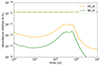 |
Fig. 3. Calculated fractional abundances of HC3S and NC3S as a function of time. Horizontal dotted lines correspond to the values observed in TMC-1 when adopting a column density of H2 of 1022 cm−2 (Cernicharo & Guélin 1987). |
The chemistry of NC3S is completely unexplored. To shed some light on the possible formation mechanism of this radical, we included several neutral–neutral reactions that could lead to NC3S, adopting a rate coefficient of 10−10 cm3 s−1. These reactions are N + HC3S, C3N + SO, C3N + S2, C3N + SH, and NH + C3S. Based on the main destruction processes of NCS (which is included in the UMIST 2022 network), we assumed that NC3S is mainly destroyed through reactions with O, H, and C atoms, and via reactions with abundant cations such as HCO+, H3O+, and H . The calculated abundance of NC3S is shown in Fig. 3, which shows that the peak calculated abundance lies 50 times below the observed value. The main formation reaction of NC3S is N + HC3S. Since in the model HC3S is the main precursor of NC3S, the abundance of the latter closely follows that of the former (see Fig. 3).
Taking into account the reduced set of reactions involving HC3S and NC3S that are included in the chemical model and the large uncertainties in the reaction rate coefficients, the predictions of the chemical model regarding these two molecules should be viewed with caution, just as an order of magnitude estimate. A careful study of the main reactions that are identified here to most influence these two molecules, namely S + C3H2 and N + HC3S, together with the reactions of HC3S and NC3S with neutral atoms would provide a more accurate view of the underlying chemical processes responsible for the presence of these two peculiar S-bearing molecules in the cold dark cloud TMC-1.
Q-band Ultrasensitive Inspection Journey to the Obscure TMC-1 Environment.
Acknowledgments
We thank Ministerio de Ciencia e Innovación of Spain (MICIU) for funding support through projects PID2019-106110GB-I00, and PID2019-106235GB-I00. We also thank ERC for funding through grant ERC-2013-Syg-610256-NANOCOSMOS. We thank the Consejo Superior de Investigaciones Científicas (CSIC; Spain) for funding through project PIE 202250I097.
References
- Agúndez, M., & Wakelam, V. 2013, Chem. Rev., 113, 8710 [Google Scholar]
- Agúndez, M., Marcelino, N., Tercero, B., et al. 2023, A&A, 677, A106 [NASA ADS] [CrossRef] [EDP Sciences] [Google Scholar]
- Cabezas, C., Agúndez, M., Marcelino, N., et al. 2022, A&A, 657, L4 [NASA ADS] [CrossRef] [EDP Sciences] [Google Scholar]
- Cabezas, C., Agúndez, M., Endo, Y., et al. 2024, A&A, 686, L3 [NASA ADS] [CrossRef] [EDP Sciences] [Google Scholar]
- Cernicharo, J. 2012, in ECLA 2011: Proc. of the European Conference on Laboratory Astrophysics, eds. C. Stehl, C. Joblin, & L. d’Hendecourt (Cambridge: Cambridge Univ. Press), EAS Publ. Ser., 251 [Google Scholar]
- Cernicharo, J., & Guélin, M. 1987, A&A, 176, 299 [Google Scholar]
- Cernicharo, J., Guélin, M., Hein, H., & Kahane, C. 1987, A&A, 181, L9 [Google Scholar]
- Cernicharo, J., Marcelino, N., Agúndez, M., et al. 2020, A&A, 642, L8 [NASA ADS] [CrossRef] [EDP Sciences] [Google Scholar]
- Cernicharo, J., Agúndez, M., Kaiser, R. J., et al. 2021a, A&A, 652, L9 [NASA ADS] [CrossRef] [EDP Sciences] [Google Scholar]
- Cernicharo, J., Cabezas, C., Agúndez, M., et al. 2021b, A&A, 648, L3 [EDP Sciences] [Google Scholar]
- Cernicharo, J., Cabezas, C., Endo, Y., et al. 2021c, A&A, 650, L14 [NASA ADS] [CrossRef] [EDP Sciences] [Google Scholar]
- Cernicharo, J., Cabezas, C., Endo, Y., et al. 2021d, A&A, 646, L3 [EDP Sciences] [Google Scholar]
- Cernicharo, J., Fuentetaja, R., Agúndez, M., et al. 2022, A&A, 663, L9 [NASA ADS] [CrossRef] [EDP Sciences] [Google Scholar]
- Cernicharo, J., Pardo, J. R., Cabezas, C., et al. 2023a, A&A, 670, L19 [NASA ADS] [CrossRef] [EDP Sciences] [Google Scholar]
- Cernicharo, J., Fuentetaja, R., Agúndez, M., et al. 2023b, A&A, 680, L4 [NASA ADS] [CrossRef] [EDP Sciences] [Google Scholar]
- Cernicharo, J., Agúndez, M., Cabezas, C., et al. 2024a, A&A, 682, L4 [NASA ADS] [CrossRef] [EDP Sciences] [Google Scholar]
- Cernicharo, J., Cabezas, C., Agúndez, M., et al. 2024b, A&A, 686, L15 [NASA ADS] [CrossRef] [EDP Sciences] [Google Scholar]
- Fossé, D., Cernicharo, J., Gerin, M., & Cox, P. 2001, ApJ, 552, 168 [Google Scholar]
- Fuente, A., Navarro, D. G., Caselli, P., et al. 2019, A&A, 624, A105 [NASA ADS] [CrossRef] [EDP Sciences] [Google Scholar]
- Fuente, A., Rivière-Marichalar, P., Beitia-Antero, L., et al. 2023, A&A, 670, A114 [NASA ADS] [CrossRef] [EDP Sciences] [Google Scholar]
- Fuentetaja, R., Agúndez, M., Cabezas, C., et al. 2022, A&A, 667, L4 [NASA ADS] [CrossRef] [EDP Sciences] [Google Scholar]
- Gordon, V. D., McCarthy, M. C., Apponi, A. J., & Thaddeus, P. 2002, ApJS, 138, 297 [CrossRef] [Google Scholar]
- Hirahara, Y., Ohshima, Y., & Endo, Y. 1994, J. Chem. Phys., 101, 7342 [Google Scholar]
- Kaifu, N., Suzuki, H., Ohishi, M., et al. 1987, ApJ, 317, L111 [NASA ADS] [CrossRef] [Google Scholar]
- Laas, J. C., & Caselli, P. 2019, A&A, 624, A108 [NASA ADS] [CrossRef] [EDP Sciences] [Google Scholar]
- Marcelino, N., Puzzarini, C., Agúndez, M., et al. 2023, A&A, 674, L13 [NASA ADS] [CrossRef] [EDP Sciences] [Google Scholar]
- McCarthy, M. C., Vrtilek, J. M., Gottlieb, E. W., et al. 1994, ApJ, 431, L127 [NASA ADS] [CrossRef] [Google Scholar]
- McCarthy, M. C., Cooksy, A. L., Mohamed, A., et al. 2003, ApJS, 144, 287 [NASA ADS] [CrossRef] [Google Scholar]
- McElroy, D., Walsh, C., Markwick, A. J., et al. 2013, A&A, 550, A36 [NASA ADS] [CrossRef] [EDP Sciences] [Google Scholar]
- Millar, T. J., Walsh, C., Van de Sande, M., & Markwick, A. J. 2024, A&A, 682, A109 [NASA ADS] [CrossRef] [EDP Sciences] [Google Scholar]
- Müller, H. S. P., Schlöder, F., Stutzki, J., & Winnewisser, G. 2005, J. Mol. Struct., 742, 215 [Google Scholar]
- Nakajima, M., Sumiyoshi, Y., & Endo, Y. 2003, J. Chem. Phys., 118, 7803 [NASA ADS] [CrossRef] [Google Scholar]
- Navarro-Almaida, D., Le Gal, R., Fuente, A., et al. 2020, A&A, 637, A39 [NASA ADS] [CrossRef] [EDP Sciences] [Google Scholar]
- Pickett, H. M. 1991, J. Mol. Spectrosc., 148, 371 [Google Scholar]
- Pickett, H. M., Poynter, R. L., Cohen, E. A., et al. 1998, J. Quant. Spectrosc. Radiat. Transf., 60, 883 [Google Scholar]
- Saito, S., Kawaguchi, K., Yamamoto, S., et al. 1987, ApJ, 317, L115 [NASA ADS] [CrossRef] [Google Scholar]
- Tercero, F., López-Pérez, J. A., Gallego, J. D., et al. 2021, A&A, 645, A37 [EDP Sciences] [Google Scholar]
- Vastel, C., Quénard, D., Le Gal, R., et al. 2018, MNRAS, 478, 5514 [Google Scholar]
- Vidal, T. H. G., Loison, J.-C., Jaziri, A. Y., et al. 2017, MNRAS, 469, 435 [Google Scholar]
- Wakelam, V., Loison, J.-C., Herbst, E., et al. 2015, ApJ, 217, 20 [NASA ADS] [Google Scholar]
- Yamamoto, S., Saito, S., Kawaguchi, K., et al. 1987, ApJ, 317, L119 [Google Scholar]
All Tables
All Figures
|
Fig. 1. Observed transitions of NC3S. Quantum numbers are indicated at the top right of each panel. The abscissa corresponds to the rest frequency. The ordinate is the antenna temperature, corrected for atmospheric and telescope losses, in millikelvins. Blank channels correspond to negative features produced when folding the frequency-switched data. The purple vertical arrows indicate the position of the three strongest hyperfine components for each transition, corresponding to Fu = Ju + 1, Ju, and Ju − 1. The red line shows the modelled spectra for NC3S with the physical parameters given in Sect. 3.1. |
| In the text | |
|
Fig. 2. Observed transitions of HC3S. Quantum numbers are indicated at the right side of each row. The abscissa corresponds to the rest frequency. The ordinate is the antenna temperature, corrected for atmospheric and telescope losses, in millikelvins. Blank channels correspond to negative features produced when folding the frequency-switched data. The Λ-doubling components e and f for each J are shown in the left and right panels, respectively. In addition, the two hyperfine components of each e and f rotational transition are resolved in our data and appear clearly detected. They correspond to Fu = Ju + 1/2 and Ju − 1/2. The red line shows the modelled spectra for HC3S with the physical parameters given in Sect. 3.3. |
| In the text | |
|
Fig. 3. Calculated fractional abundances of HC3S and NC3S as a function of time. Horizontal dotted lines correspond to the values observed in TMC-1 when adopting a column density of H2 of 1022 cm−2 (Cernicharo & Guélin 1987). |
| In the text | |
Current usage metrics show cumulative count of Article Views (full-text article views including HTML views, PDF and ePub downloads, according to the available data) and Abstracts Views on Vision4Press platform.
Data correspond to usage on the plateform after 2015. The current usage metrics is available 48-96 hours after online publication and is updated daily on week days.
Initial download of the metrics may take a while.