| Issue |
A&A
Volume 648, April 2021
|
|
|---|---|---|
| Article Number | A106 | |
| Number of page(s) | 13 | |
| Section | The Sun and the Heliosphere | |
| DOI | https://doi.org/10.1051/0004-6361/202140277 | |
| Published online | 21 April 2021 | |
The configuration and failed eruption of a complex magnetic flux rope above a δ sunspot region⋆
1
Planetary Environmental and Astrobiological Research Laboratory (PEARL), School of Atmospheric Sciences, Sun Yat-sen University, Zhuhai, Guangdong 519082, PR China
e-mail: This email address is being protected from spambots. You need JavaScript enabled to view it.
2
CAS center for Excellence in Comparative Planetology, Hefei, PR China
3
Astrophysics Research Centre, School of Mathematics and Physics, Queen’s University, Belfast BT71NN, UK
4
CAS Key Laboratory of Geospace Environment, Department of Geophysics and Planetary Sciences, University of Science and Technology of China, Hefei, Anhui 230026, PR China
5
Institute of Space Science and Applied Technology, Harbin Institute of Technology, Shenzhen, PR China
6
CAS Key Laboratory of Lunar and Deep Space Exploration, National Astronomical Observatories, Chinese Academy of Sciences, Beijing 100012, PR China
Received:
2
January
2021
Accepted:
10
February
2021
Abstract
Aims. We aim to investigate the configuration of a complex flux rope above the δ sunspot region in the National Oceanic and Atmospheric Administration AR 11515 and its eruptive expansion during a confined M5.3-class flare.
Methods. We studied the formation of the δ sunspot using the continuum intensity images and photospheric vector magnetograms provided by the Helioseismic and Magnetic Imager on-board the Solar Dynamics Observatory (SDO). We employed the extreme-ultraviolet and ultraviolet images provided by the Atmospheric Imaging Assembly on-board SDO and the hard X-ray emission recorded by the Reuven Ramaty High-Energy Solar Spectroscopic Imager to investigate the eruptive details. The coronal magnetic field is extrapolated from the photospheric field using a nonlinear force free field (NLFFF) method, based on which the flux rope is identified through calculating the twist number Tw and squashing factor Q. We searched the null point via a modified Powell hybrid method.
Results. The collision between two newly emerged spot groups form the δ sunspot. A bald patch (BP) configuration forms at the collision location between one umbra and the penumbra, above which a complex flux rope structure is identified. The flux rope has a multilayer configuration, with one compact end and the other end bifurcating into different branches. It has a non-uniform Tw profile, which decreases from the core to the boundary. The outmost layer is merely sheared. A null point is located above the flux rope. The eruptive process consists of precursor flarings at a v-shaped coronal structure, rise of the filament, and brightening below the filament, corresponding well with the topological structures deduced from the NLFFF, including a higher null point, a flux rope, and a BP and a hyperbolic flux tube (HFT) below the flux rope. Two sets of post-flare loops and three flare ribbons in the δ sunspot region further support the bifurcation configuration of the flux rope.
Conclusions. Combining the observations and magnetic field extrapolation, we conclude that the precursor reconnection, which occurs at the null point, weakens the overlying confinement to allow the flux rope to rise, fitting the breakout model. The main phase reconnection, which may occur at the BP or HFT, facilitates the flux rope rising. The results suggest that the δ spot configuration presents an environment prone to the formation of complex magnetic configurations that work together to produce activities.
Key words: sunspots / Sun: magnetic fields / Sun: activity / Sun: corona / Sun: flares / Sun: filaments / prominences
Movies associated to Figs. 2 and 6 are available at https://www.aanda.org
© ESO 2021
1. Introduction
Sunspots appear as dark spots on the photosphere in white light observation, reflecting the convection inhibition caused by the concentrations of strong magnetic flux that constitute the solar active regions (ARs). They usually appear as groups, exhibiting various configurations. The most complex type is called δ sunspot, which is manifested as two umbrae of opposite polarities sharing a common penumbra (Künzel 1960). Observations reveal that regions harboring δ spots are productive in solar flares and coronal mass ejections (CME, Shi & Wang 1994; Sammis et al. 2000; Takizawa & Kitai 2015; Toriumi et al. 2016; Toriumi & Wang 2019), which are the two most spectacular phenomena in the solar atmosphere. A few common features observed in δ spot regions are considered to account for their high productivity. For example, the opposite-signed polarities in these regions tend to be stronger and more compact, forming high-gradient, strongly-sheared polarity inversion lines (PILs), which indeed indicate the non-potentiality of the magnetic field (Hagyard et al. 1984; Tanaka 1991; Schrijver 2007). Shearing motions along the PILs and sunspot rotations also frequently appear. They are suggested to be able to shear or twist the field (Hagyard et al. 1984; Leka et al. 1996; Fan 2009; Yan et al. 2015). The non-potential magnetic field, in combination with photospheric motions, may create an environment apt to the magnetic reconnections and eruptions (Fang & Fan 2015).
The formation conditions of δ spots were summarized in three categories by Zirin & Margaret (1987): they can form when intertwined bipoles emerge at once, when satellite spots emerge into pre-existent spot regions, and when different spot groups collide. Numerical simulations suggest that the formation of δ spots results from the emergence of twisted magnetic flux tubes from the convection zone, which can induce shearing motions and sunspot rotations self-consistently (Leka et al. 1996; Fang & Fan 2015; Toriumi & Hotta 2019). After formation, the coronal counterparts of δ spot regions exhibit complex configurations as well, sometimes in the form of sigmoidal structures, which are considered as coronal proxies of the magnetic flux rope (e.g., Joshi et al. 2018). The flux rope is a magnetic structure consisting of a set of helical field lines collectively wrapping around an axis with more than one full turn (Cheng et al. 2017, and references therein).
It is suggested that the magnetic flux rope is a fundamental structure in solar eruptions (Liu 2020, and references therein). For example, although flares and CMEs appear differently, with the former being local enhancements of electromagnetic radiation and the latter being more global expulsions of magnetized plasma, it is suggested that they are different manifestations of a same process involving the eruption of magnetic flux ropes (Forbes 2000). In the classical two-dimensional (2D) scenario of the standard flare model, the flux rope erupts to form the main body of the CME, generating current sheet at the CME wake through the stretching of the strapping field. The reconnection manifested as flare occurs at the current sheet (Carmichael 1964; Sturrock 1966; Hirayama 1974; Kopp & Pneuman 1976; Shibata et al. 1995). The standard flare model has been extended to the three-dimensional (3D) space (Aulanier et al. 2012; Janvier et al. 2013), in which the current sheet where the flare occurs seems to have formed around the hyperbolic flux tube (HFT, Titov et al. 2003). The exact trigger of the eruption is explained by other models that can be roughly divided into two categories: magnetic reconnection model and ideal magnetohydrodynamics (MHD) instability model (Chen 2011, and references therein). For the former, magnetic reconnection may occur above the sheared arcades at the null point as in the breakout model (Antiochos et al. 1999), or below the sheared arcades as in the tether-cutting model (Moore et al. 2001). In these scenarios, the flux rope forms on the fly. On the contrary, pre-existent flux rope is usually required in ideal MHD instability models, such as kink instability and torus instability models (Török et al. 2004; Kliem & Török 2006). The above models are supported by observations (Cheng et al. 2017, and references therein).
Observationally, we are not able to “see” the coronal flux rope directly since there is no direct measurement of the coronal magnetic field at present. A few observable entities such as sigmoids (Canfield et al. 1999), filaments (Martin 1998), and hot channels (Zhang et al. 2012) are considered as proxies of the flux ropes (Liu 2020, and references therein). In situ observations of interplanetary magnetic clouds also give hint to the configuration of the flux ropes (Hu et al. 2014; Wang et al. 2018a). On the other hand, various methods have been developed to reconstruct the 3D coronal magnetic field (Guo et al. 2017; Wiegelmann et al. 2017, and references therein), based on which one can locate and analyze the flux rope (Liu et al. 2016). It is found that the flux rope in reconstructed field presents as strong twisted regions wrapped by a boundary of quasi-separatrix layers (QSLs, Titov 2007), which is in fact natural according to the definition of the magnetic flux rope (Liu et al. 2016). Besides the coherent structure of one flux rope, the field lines of which have similar rotational patterns (Liu et al. 2016), more complex configurations are found in the ARs, such as a double-decker configuration with one flux rope atop the other one (Kliem et al. 2014), intertwined double-decker flux rope (Mitra et al. 2020), braided flux ropes (Awasthi et al. 2018), and the coexisting flux rope and sheared arcades along one filament (Guo et al. 2010).
Overall, a δ sunspot, which indicates a non-potential configuration, and a flux rope, which is a highly non-potential structure in the corona, both play important roles in solar eruptions. A detailed study of the magnetic flux rope in the δ sunspot region -including its formation, configuration, and eruption, and, moreover, the role that the δ spot configuration plays in the above process- is necessary to understanding solar eruptions. A few observations have related the two explicitly. Jiang et al. (2012) reported that a highly twisted filament channel was formed above the δ sunspot in National Oceanic and Atmospheric Administration (NOAA) AR 11158. With the aid of coronal field extrapolation, Mitra et al. (2018) also found that the flux ropes successively erupted from AR 12673 were formed in the δ sunspot of the AR. In this work, we investigated the configuration and failed eruption of a complex flux rope structure above the central δ spot of AR 11515. The AR is very prolific in flares and CMEs and has been intensively studied (Louis et al. 2014; Jing et al. 2014; Wang et al. 2014, 2018b). The flux rope we studied is related to a confined M5.3-class flare that occurred on 2012 July 4. The paper is structured as follows: in the next section, we describe the data and method used; the results are presented in Sect. 3; and we discuss the implication of this work in Sect. 4.
2. Data analysis
We used the photospheric continuum intensity maps and vector magnetograms provided by the Helioseismic and Magnetic Imager (HMI, Scherrer et al. 2012) on-board the Solar Dynamics Observatory (SDO, Pesnell et al. 2012) to investigate the evolution of the δ sunspot. HMI generates the vector magnetograms with a plate scale of 0 5 and a cadence of 12 minutes, based on which the ARs are automatically extracted and tracked. Here, the data segment deprojected to a cylindrical equal area (CEA) coordinate is used (Bobra et al. 2014). The data segment is released as HMI.sharp_cea_720s series (Hoeksema et al. 2014). Using the field data, we calculated the unsigned magnetic flux via
 (1)
(1)
in which Bz is the vertical component of the magnetic field, and ds is the area of the pixel. Since the magnetic field measurement suffers from a severe projection effect when near the solar limb (Petrie 2015), we only calculated Φ when the AR is not far from the disk center, that is, in the region between the Stonyhurst longitude from 60°E to 60°W.
We employed the ultraviolet (UV) and extreme-ultraviolet (EUV) images provided by the Atmospheric Imaging Assembly (AIA, Lemen et al. 2012) on-board SDO to inspect the details of the M5.3-class flare. The data has a plate scale of 0 6 and a cadence up to 12s. The hard X-ray (HXR) emission of the flare is recorded by the Reuven Ramaty High-Energy Solar Spectroscopic Imager (RHESSI, Lin et al. 2002). We used the detectors 1F, 3F, 4F, 5F, 6F, 7F, and 8F to reconstruct the HXR sources at 12–25 KeV by the CLEAN algorithm (Hurford et al. 2002).
We studied the coronal magnetic field of the region by extrapolating the photospheric vector magnetogram using a nonlinear force free field (NLFFF) method (Wiegelmann 2004; Wiegelmann et al. 2012). Since the photosphere is not necessarily force free, the photospheric magnetogram used as the input of the extrapolation needs to be preprocessed to reduce possible force, torque, and other noises (Wiegelmann et al. 2006). Three dimensionless parameters, the flux balance parameter, the force balance parameter, and the torque balance parameter, are calculated to quantify the quality of the preprocessed magnetogram. We also calculated the fractional flux ratio and the weighted angle between current (J) and magnetic field (B) to check the divergence-freeness and force-freeness of the extrapolated field (Derosa et al. 2015).
Based on the extrapolated field, we calculated the twist number Tw and squashing factor Q using the code1 developed by Liu et al. (2016) to identify the flux rope, the cross section of which is manifested as areas of high Tw wrapped by high Q boundaries (Liu et al. 2016). Tw measures the number of turns that two extremely close field lines wind around each other, and it is computed through the equation (Berger & Prior 2006; Liu et al. 2016)
 (2)
(2)
in which α denotes the force free parameter and dl denotes the elementary length of the field line. Q quantifies the local gradient of the magnetic connectivity. For an arbitrary field line, its two footpoints define a mapping: r1(x1, y1)→r2(x2, y2), the Jacobian matrix of which is
![Mathematical equation: $$ \begin{aligned} \displaystyle D_{12}=\bigg [\frac{\partial \boldsymbol{r_2}}{\partial \boldsymbol{r_1}}\bigg ]=\Bigg ( \begin{matrix} \frac{\partial x_2}{\partial x_1} \frac{\partial x_2}{\partial { y}_1}\\ \frac{\partial { y}_2}{\partial x_1} \frac{\partial { y}_2}{\partial { y}_1} \end{matrix} \Bigg ) \equiv \Bigg ( \begin{matrix} a&b\\ c&d \end{matrix} \Bigg ). \end{aligned} $$](/articles/aa/full_html/2021/04/aa40277-21/aa40277-21-eq5.gif) (3)
(3)
The squashing factor is then defined as
 (4)
(4)
in which Bn, 1(x1, y1) and Bn, 2(x2, y2) are components perpendicular to the plane of the footpoints (Titov et al. 2002; Liu et al. 2016). High Q regions usually indicate the QSLs, a thin volume where the connectivity of magnetic field lines shows drastic change. The electric current is easily to be accumulated at the QSLs, favoring magnetic reconnection. For a coherent flux rope possessing some degree of cylindrical symmetry, we can further take the field line owning the extremum Tw of the flux rope as a reliable proxy of its axis (Liu et al. 2016). We also searched for the null point by solving the equation
 (5)
(5)
in which i = x, y, z, using a modified Powell hybrid method2 (Demoulin et al. 1994). We then visualized the NLFFF field lines via a software called PARAVIEW3, which provides an interactive environment for visualization.
3. Results
3.1. Formation of the δ sunspot
When it appears at the east limb on 2012 June 27, NOAA AR 11515 is already developed with a complex βγ configuration. It has unsigned magnetic flux as large as 3.5 × 10²² Mx when passing the Stonyhurst longitude 60°E on 2012 June 28 (see Fig. 1a). About three days later, a new episode of flux emergence initiates in the western part of the AR, which transports more than 4.5 × 10²² Mx to the AR before it rotates out of view. During the emergence, a δ sunspot is formed in the middle of the AR (Figs. 1b,c). An M5.3 class flare, accompanied by the failed eruption of a filament, takes place in the δ sunspot region from 09:47 to 09:57 UT on 2012 July 04 (Figs. 1d–f). The reason for the failure of the eruption was studied in Li et al. (2019). Here, we mainly focus on the formation of the δ sunspot, the detailed configuration of the pre-eruption flux rope and the magnetic topology accounting for the eruption characteristics.
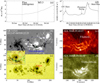 |
Fig. 1. Overview of AR and the flare. (a) Temporal evolution of the unsigned magnetic flux Φ of the AR. Φ is calculated from 2012 June 28 13:00 to 2012 July 7 11:10, i.e., when the center of the AR has Stonyhurst longitude less than 60°. The two vertical-dashed lines mark the onset instants of the flux emergence and the flare. (b) Bz component of the photospheric vector magnetic field of the AR at 09:22 on 2012 July 4, with white and black colors indicating the positive and negative polarities, respective, saturating at ±1200 G. (c) Continuum image of the AR. The blue rectangle in (b) and (c) marks the field of view (FOV) of panels e, f, and Fig. 2. The green rectangle marks the FOV of Fig. 3. The continuum intensity in the blue region is further shown in the inset (c1), with contours of Bz overplotted. The contour levels are −1000, −100, 100, and 1000 Gauss, with positive (negative) values shown in purple (cyan). The red circle in (c) indicates the δ sunspot region. (d) GOES flux of the M5.3 class flare. The three arrows indicate a small C9.7-class flare, and the precursor and main phase of the M5.3-class flare. See details in Sects. 3 and 4. (e) One snapshot in the AIA 304 Å passband prior to the flare, showing the filament. (f) One snapshot in the AIA 1600 Å passband, showing multiple ribbons during the flare. |
While the flux emergence started on 2012 July 01, the δ sunspot was not formed until 2012 July 04. We present the emergence period relevant to the spot formation in Fig. 2. On 2012 July 03, a newly emerged bipole, bipole1, drifted from the west to the middle of the AR (Fig. 2a1), followed by another small bipole, bipole2. The two polarities of bipole1 (N1 and P1) are observed as developed sunspots consisting of the umbra and penumbra in the continuum image (Fig. 2a2), while the two polarities of bipole2 (N2 and P2) are presented as pores. As emergence goes on, the polarity N2 moves to the east, and finally collides with P1 (Figs. 2b1–e1). After collision, the flux emergence continues. Due to the existence of N2, some newly emerged positive flux of bipole1 forms a small patch that is isolated from the original P1, being located at the north of N2. We call the new patch  (indicated by a cyan arrow in Figs. 2f1–h1), and the old, large P1,
  (Figs. 2f1–h1).
  appears as a patch of penumbra in the continuum image (Figs. 2f2–h2). Simultaneously, N2 also develops into a sunspot in the continuum image, which together with
  and
and  form the δ sunspot configuration (enclosed by the red circle in Fig. 2h2). We note that P2 is still dispersed, consisting of small flux patches that appear as small pores in the continuum image.
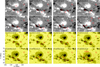 |
Fig. 2. Formation of δ sunspot. Panels a1–h1 display the photospheric Bz magnetograms, with Bz saturating at ±1200 G, while panels a2–h2 are the continuum images. Label PA denotes a pre-existent positive polarity. N1 and P1 indicate the negative and positive polarities of bipole1, respectively, while N2 and P2 are for bipole2. |


3.2. Configuration of the flux rope
We further selected a moment (2012-07-04T09:22 UT) to investigate the pre-flare magnetic condition above the δ sunspot region. The photospheric vector magnetic field and the extrapolated coronal field are checked, shown in Figs. 3–5. We find a sheared PIL formed between  and the group of N1 and N2 (green line in Fig. 3a), which is obtained via drawing the contour of Bz = 0 on the Bz map directly. The pixels of the PIL all have shear angle (S) larger than 55° (Fig. 3b), indicating the high non-potentiality here. S is the angle between observed field (BObs) and the potential field (BPot), calculated by equation (Bobra et al. 2014)
 (6)
(6)
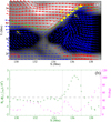 |
Fig. 3. Bald patch between N2 and |


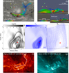 |
Fig. 4. Configuration of the flux rope that is identified in the extrapolated NLFFFs. (a)–(b) The flux rope seen from two different views. The iridescence colors vary with the strength of the field. Panel a has the same FOV as Fig. 2. The inset (b1) shows the field lines passing through the BP specifically. The yellow-dashed rectangle marks the northern branches of the flux rope, while the pink one is for the southern branch. The photospheric Bz saturates at ±2000 G in these panels, with white (black) patches indicating the positive (negative) polarities. (c)–(e) Distribution of logarithmic Q, Tw, and in-plane field vector in a vertical plane, which is perpendicular to the local apex of the possible axis proxy. The red triangles indicate the local extremum of Tw, i.e., the location where the possible axis proxy threads the plane. The position of the plane is indicated by the semi-transparent cut in panel b. (f) Image of the AIA 304 Å passband, showing the filament. The white line denotes the estimated axis of the flux rope from NLFFFs. (g) The image of the AIA 131 Å passband, showing two sets of loops overlying the northern and southern branches of the flux rope. The colored dashed rectangles enclose the same regions as the ones in panel a. Panels a, f, and g have the same FOV. |
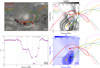 |
Fig. 5. Different layers of the flux rope. (a) Representative field line from each layer. The panels have the same FOV as Fig. 2. The photospheric Bz saturates at ±2000 G, with white (black) patches indicating the positive (negative) polarities. (b) Profile of Tw along the black line in d, which is parallel to the photopshere and passing the extremum point. The vertical-dashed lines correspond to the black dots in panel d. The digits mark the layers of the flux rope. (c)–(d) Distributions of the logarithmic Q and Tw in the same plane indicated in Fig. 4b. The position of the plane is also indicated by a white line in panel a, with the white dot denoting the start point of the plane. The representative field lines from each layer are overplotted. The solid parts of the lines are in front of the plane (seen along the line of sight), while the dashed parts are behind the plane. The colored dots mark the positions where the field lines thread the plane. The black dots indicate locations where the horizontal black line intersects with the high Q boundaries. |
The potential field is computed by a frourier transformation method (Alissandrakis 1981). Moreover, we find a bald patch (BP) formed at the interface between N2 and  (yellow dots in Fig. 3a), that is, between one umbra and the penumbra of the δ spot. BP is a configuration at which the field lines are tangent to the photosphere and concaved up, showing a inverse configuration that points from the negative polarity to the positive polarity (see blue vectors in Fig. 3a). It can be identified through the discriminant (Titov et al. 1993, see Fig. 3b here)
 (7)
(7)
where Bh and Bz denote the horizontal and vertical components of the magnetic field. BP usually belongs to the bald patch separatrix surface (BPSS), which is prone to the formation of a flux rope. Such configuration is found to be a preferred location for current accumulation in the corona and thus magnetic reconnection (Titov & Démoulin 1999).
We then searched for the flux rope in the extrapolated NLFFF. The quality of the preprocessed photospheric magnetogram was checked firstly. The values of the dimensionless parameters (see Sect. 2) are presented in Table 1. It is found that the value of the flux balance parameter slightly increases after preprocessing, but is still of the order of 10−2, indicating that the magnetic flux of the magnetogram is basically balanced, either before or after the preprocessing. The values of the force-balance and torque-balance parameters are of the order of 10−2 after preprocessing, decreasing by an order of magnitude compared to the values before preprocessing, suggesting that the force and torque on the magnetogram are significantly reduced. We also checked the quality of the extrapolation. It is found that the value of the fractional flux ratio is 2.03 × 10⁻³, and the weighted angle between J and B is 9.07°. While the former value is small, the latter is about 2° larger than the values of some reported NLFFF results (Liu et al. 2017; Mitra et al. 2020). Nevertheless, both values are not large, suggesting that the degree of the divergence-freeness and force-freeness of the extrapolation is acceptable.
Values of the dimensionless quality parameters of the photospheric magnetogram before and after preprocessing.
We do find a flux rope structure (shown in Figs. 4a,b) above the δ spot region after having checked the Tw and Q distributions in a series of vertical planes across the PIL. The flux rope displays a complex configuration consisting of different branches, with one compact end rooted in N1, and the other end bifurcating into different branches that are rooted in  , discrete flux patches of P2, and also part of the periphery of the pre-existent PA. In the following, we label the branch rooted in
  as the southern branch of the flux rope (indicated by a pink rectangle in Fig. 4a), since
  is located in the southern part of the AR, and the ones rooted in P2 and PA (enclosed in a yellow rectangle) as northern branches. The bottom of the flux rope touches the photosphere at the BP between N2 and
  (see the field lines passing through the BP in Fig. 4b1). We further tried to identify the axis of the flux rope through inspecting the local extremums of the Tw maps. A field line possessing the local maximum in all Tw maps we inspected is found, which may be deemed as the proxy of the flux rope axis (Liu et al. 2016). Q, Tw, and the in-plane field vectors in a vertical plane normal to the tangent line of the apex (local peak of a curve) of the possible axis proxy are displayed in Figs. 4c–e. Unsurprisingly, the cross-section of the flux rope is manifested as the strong twisted region wrapped by high Q boundary. Moreover, it exhibits a more complex, onion-like configuration, consisting of different layers that are separated by different high Q boundaries. Most of the in-plane field vectors are found rotating around the possible axis proxy (denoted by the red triangles in Fig. 4), except the ones below the possible axis. This may be because the flux rope has bifurcated ends, which indicates that it is not strictly coherent, so there may be a few field lines that have slightly different rotational patterns from the other field lines at some locations. We also compared the flux rope and the filament observed in AIA 304 Å passband (Fig. 4f). It is found that the eastern part of the flux rope coincides with the filament to a large extent. The western part of the filament is covered by higher loops, which makes the direct comparison unachievable. Moreover, we find two sets of loops in the AIA 131 Å passband, which overlie the southern and northern branches of the flux rope, respectively (Fig. 4g).
We further checked the detailed properties of each layer of the flux rope (Fig. 5). Typical field lines of each layer are randomly chosen to show. It is found that Tw decreases gradually from the core to the boundary. The core layer (layer 5), where the possible axis proxy threads, owns the largest twist with almost uniform Tw as high as −3.8 (Fig. 5b). The field lines of the layer are rooted in the polarities N1 and  (see the blue line in Fig. 5). The outer layer, layer 4, has lower Tw roughly ranging from −3 to −2.7. The field lines of this layer originate from the polarity
  , then go into N1 (see the green line in Fig. 5). Some of the field lines further pass though
  and N2 (the BP). Layer 3 has Tw ranging from −3 to −1.5. Its field lines span the longest distance, rooted in polarities N1 and remote
  (see the orange line in Fig. 5). Layer 2 owns Tw in the range of −2.4 to −1. Its field lines are found rooted in N1 and
  (see the pink line in Fig. 5). Some of the field lines also pass through the BP. The outermost layer (layer 1) is the least twisted part, having Tw ranging from −0.9 to −0.5 (see the red line in Fig. 5). Its field lines are rooted in polarities N1 and
  , with some of them also passing through the BP. They indeed do not meet the criterion of the field lines belonging to a typical flux rope, which should wind at least one full turn. However, they are intertwined with the more twisted inner layers, together forming an inseparable whole structure. We thus call this structure a complex flux rope.
3.3. Topological origin of the eruption characteristics
The flare is accompanied by the failed eruption of a filament. Taking the filament as a proxy of the flux rope, its failed eruption suggests that the flux rope experiences an eruptive expansion during the flare. The Lorentz force during the eruption is nonzero, making the in-eruption NLFFF extrapolation unreliable. We thus checked the eruption characteristics observed in various passbands to deduce the eruptive details of the flux rope. We selected three AIA passbands, the hot 131 Å (∼10 MK), cool 304 Å (∼50 000 K), and the UV 1600 Å (∼10 000 K), to show the eruptive details (Fig. 6). The GOES soft X-ray (SXR) flux shows that the flare starts from 07-04T09:47 UT, peaks at 09:55, and ends at 09:57 (Fig. 1d). Besides, from around 09:35 to 09:47, a small “bump” appears on the SXR curve (Fig. 1d), suggesting that some mild flarings, that is, a phase of mild reconnection, occur prior to the recorded flare. This kind of gradual buildup of the SXR flux prior to the main flare, which is distinct from the rapid increasing of the SXR flux during the main flare, is called a precursor phase (Zhang & Dere 2006; Mitra & Joshi 2019). Furthermore, in the hot 131 Å passband (Figs. 6a1–b1), an inclined v-shaped structure brightens. The structure seems to consist of two sets of loops, with two far sides rooted in  and dispersed P2, and the other two close sides somehow intersecting at higher altitude to form the cusp of the v (Fig. 6a1). In the RHESSI observation, an HXR source at the 12–25 keV energy bands is found to be centered at the cusp. The EUV brightening and HXR source further support that there is a phase of precursor reconnection occurring prior to the main flare. We call this phase of reconnection reconnection1.
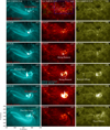 |
Fig. 6. Eruptive characteristics of the flare. (a1)–(f1) Eruptive details observed by the AIA 131 Å passband. The white arrows in (f1) point out two sets of post-flare loops. The two dashed boxes in (f1) are the same as the ones in Fig. 4g, enclosing the northern and southern sets of loops. The polarities |

After the precursor brightening, a filament bundle starts to rise slowly from around 09:46 (see Figs. 6c2–d2 and associated movie). The footpoints of the filament brighten during the rise, forming a HXR source at the eastern footpoint (Fig. 6d2). From around 09:52, another brightening occurs below the rising filament, which is visible in both 131 Å and 304 Å passbands, as well as in the 1600 Å passband, forming a new HXR source (Fig. 6e1). This is the main phase reconnection generating the peak SXR flux of the flare. We call this phase of reconnection reconnection2. Following reconnection2, the filament continues to rise and finally stops without forming a CME. After the failed eruption, two sets of nearly-potential post-flare loops appear above the δ spot region, with one set connecting P2 (also part of the periphery of PA) and the group of N1 and N2 (enclosed in a yellow rectangle in Fig. 6f1), and the other set connecting  and the group of N1 and N2 (enclosed in a pink rectangle in Fig. 6f1). Three elongated ribbons appear at the footpoints of the loops in the 1600 Å passband (Fig. 6f3). Besides this, there is a remote ribbon brightening during the flare, located at the east of the AR, which seems to be connected with the core region by some sheared loops (Figs. 6d1 and d3).
The inclined v-shaped structure, which shows a HXR source centered at its cusp during the flare, strongly suggests that there might be a null point. We thus searched the pre-eruption NLFFFs using the method described in Sect. 2, and do find a null point above the flux rope (Fig. 7). The configuration of the null point is very similar to the classical null associated with fans and spines (Priest & Titov 1996). The outer spine here is rooted in the remote negative polarity, while the inner spine is rooted in N2. The only exception here is that the field lines of the fans are rooted in two disconnected polarity patches,  and P2, differently from the circular fan of the classical configuration. The null is manifested as the intersection of two high Q lines (indicated by a red star in Fig. 7c) in a vertical plane across it. Moreover, the flux rope is exhibited as an inverse-teardrop-shaped structure in this plane, similarly to what is seen in Fig. 4, but with a HFT configuration at the bottom. HFT is a configuration where two QSLs intersect, which are prone to current accumulation, and thus reconnection (Titov et al. 2003).
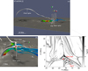 |
Fig. 7. Null point above the flux rope, which is marked as a red star. (a)–(b) Different view of the null point. Magnetic field lines traced from different topological structures are shown in different colors. The iridescent lines belong to the flux rope, while the gray lines are for the coronal configurations associated with the null point. (c) The distribution of logarithmic Q in a vertical plane crossing the magnetic null. The position of the plane is indicated by a semi-transparent cut in panel a. The photospheric Bz in panels a and b saturates at ±2000 G. |
We further show the AIA observations and the magnetic topological structures together in Fig. 8 to better explain the eruptive process. The v-shaped structure in the 131 Å image (shown in red in Fig. 8a), that is, the location where the first phase of the reconnection occurs, generally coincides with the null point identified in the reconstructed coronal NLFFFs (Fig. 8b). The only difference is that the sheared loops connecting the core region and the remote region in the 131 Å passband deviate from the outer spine in the NLFFFs. The former are rooted in the more northern part of the remote negative polarity, while the latter is rooted in more southern region. This may result from the limitations of the NLFFF model and the projection effect since the NLFFF image is in the CEA coordinate, while the AIA images are in the CCD coordinate. The main phase reconnection seems to occur below the null point (show in green in Fig. 8a). The position of the two sets of post-flare loops (shown in blue in Fig. 8a) and the three main flare ribbons (white contours in Fig. 8a) correspond well to the bifurcated branches of the pre-eruption flux rope. Specifically, the northern set of the post-flare loops connects P2 (also part of the periphery of PA) and the group of N1 and N2, while the northern branches of the flux rope are also rooted in P2 and N1, passing through N2 at the BP (Fig. 8b). The southern set of the loops connects  and the group of N1 and N2, while the southern branch of the flux rope is also rooted in
  and N1 (also passing through N2). The three ribbons are located in P2 (also part of the periphery of PA), the group of N1 and N2, and
  as well. These suggest that the bifurcated flux rope is involved in the failed eruption. The ejective expansion of different branches of the flux rope stretches different sets of strapping field (see Fig. 4g), forming two sets of post-flare loops and three flare ribbons that are rooted near the footpoints of the flux rope branches. The results support the notion that the extrapolated bifurcated flux rope generally coincides with the observation.
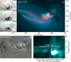 |
Fig. 8. Comparison between the eruptive characteristics and the magnetic topology. (a) Composite image of AIA 131 Å observations at three different times. The observation at 09:42 is shown in red, the one at 09:52 is shown in green, and the one at 10:02 is shown in blue, which display the coronal null, the main phase of reconnection, and the post-flare loops, respective. The three insets at the left are the negative images at the three times. The white contours outline the flare ribbons in the 1600 Å observation. The blue rectangle has the same FOV as the one in Fig. 1b. White-dashed line indicates the position of the slice used in panel c. White dot marks the start of the slice. (b) Flux rope (shown in iridescence) and the magnetic field lines of the configurations associated with the null (shown in gray) in the extrapolated NLFFF. Panel b has roughly the same FOV as panel a. (c) Time-distance plot of the slice, showing the two phases of reconnection and the rise of the filament. |
We also present the time-distance diagram of a slice (white dotted line in Fig. 8a) extracted from the 131 Å images to better see the sequence of the eruption characteristics (Fig. 8c). The slice runs across the filament. It is seen that before the filament rises, there is a phase of mild brightenings occurring above the filament, which corresponds to the precursor reconnection at the null point. After the start of the filament rising, a second phase of strong flarings occurs below the filament, which apparently corresponds to the main phase reconnection. The diagram confirms the sequence of the eruption characteristics, that is, reconnection1 occurs at the null at first, followed by the rise of the filament, and then reconnection2 occurs below the filament, after which point the filament continues to rise and finally stops. These suggest that the trigger of the failed eruption is more likely to be the breakout reconnection at the null, which weakens the confinement of the strapping field and causes the rise of the filament. The main phase reconnection occurring below the filament gives positive feedback to the rising filament. Since the main reconnection is visible in various passbands, even in 1600 Å, which monitors the photosphere and the lower chromosphere, it is very possible that it occurs rather low, and hence might be associated with the pre-existent BPSS or the HFT below the flux rope.
4. Summary and discussion
In this work, by combining the multiple wavelength observations and the coronal magnetic field extrapolation, we investigated the configuration of a complex flux rope structure in NOAA AR 11515, and its failed eruption during a confined M5.3-class flare. It is found that the flux rope is formed right above the δ spot region, consisting of multiple layers, with its cross-section exhibiting an onion-like configuration. Above the flux rope, a null point is identified. The eruption process suggests that the precursor reconnection occurs at the null point, which is manifested as an inclined v-shaped structure. It weakens the overlying confinement, causing the slow rise of the flux rope, which is indicated by a filament. The main phase of reconnection occurs below the flux rope, probably at the BPSS or HFT, facilitating the rise of the flux rope. The eruptive expansion of the flux rope finally stops without forming a CME.
The δ sunspot is formed through the collision between two spot groups that are newly emerged near the pre-existent spot regions (PA). The collision occurs between one umbra and the penumbra, which become part of the δ sunspot later. A bald patch configuration is found formed at the collision location. The identified flux rope is attached to the photosphere at the BP (see Fig. 4b1). The result suggests that the δ sunspot configuration, where two umbrae are located close in the same penumbra that contain opposite-signed polarities huddling together, naturally creates an environment prone to the formation of the flux rope. The detailed formation of the flux rope is beyond the scope of this paper. We do not identify flux ropes in the extrapolated coronal field before 09:00 on July 4, but we do find a smaller flare (C9.7-class) that occurs from around 09:00 to 09:09, during which small-scale brightenings are observed in the BP region in 1600 Å, accompanied by brightenings of nearby coronal loops (visible in 131 Å) that are associated with two other small ribbons (see the movie associated with Fig. 6). It is suggested that the flux rope may be formed or built-up in confined flares prior to large eruptions (Guo et al. 2013; Joshi et al. 2016; James et al. 2017; Liu et al. 2018a, 2019), most probably via magnetic reconnection between different sheared loops in a tether-cutting manner (Syntelis et al. 2019). Therefore, the flux rope here may be formed through small-scale reconnection between different sheared field lines near the BPSS.
The flux rope consists of multiple layers, exhibiting an onion-like configuration in the Tw and Q maps of its cross section. One of the flux rope’s ends is compact, rooted in one negative polarity, while the other end bifurcates into different branches rooted in discrete positive polarity patches, indicating that the connectivities of the different branches change drastically to form the QSLs around each layer. The twist profile of the flux rope is not uniform, with Tw decreasing from the core to the boundary. The core has a twist as high as 3.8 turns. This is consistent with some in situ observations of interplanetary magnetic clouds, which exhibit a highly twisted core enclosed by a less twisted envelope (Hu et al. 2014; Wang et al. 2018a). The outmost layer of the flux rope here has a twist of less than one full turn, which indeed is “sheared” rather than “twisted”. This is similar to the observation reported in Guo et al. (2010), in which a flux rope and sheared arcade sections are found coexisting along one filament. The difference here is that the sheared layer is intertwined with the other twisted branches of the flux rope, forming a complex structure. Similar but different configurations of complex flux rope have been reported. For example, Awasthi et al. (2018) identified a complex structure consisting of multiple flux ropes or flux bundles braiding about each other in extrapolated NLFFFs. Hou et al. (2018) also concluded that a multi-flux-rope system is formed through interactions between different emerging dipoles. Overall, the observations suggest that the flux rope in δ sunspot region, or, more generally, in multipolar regions, may have quite a complex configuration due to the interaction between adjacent polarities and may be different from the simple configuration of a single coherent flux rope in bipolar regions. The latter is often presented in numerical simulations (e.g., Gibson et al. 2004; Aulanier et al. 2010).
Since the NLFFF assumption does not stand during the flare, we compared the pre-eruption magnetic condition and the eruption characteristics observed by various passbands to deduce the details of the eruptive expansion of the flux rope. The v-shaped structure that brightens prior to the rise of the filament corresponds well with the null point identified in the NLFFFs, suggesting a precursor phase of reconnection occurs at the null, which is also evidenced by the mild enhancement of the SXR flux and the HXR source at the cusp of the v. The precursor may have triggered the flux rope to rise by weakening the confinement of the overlying field, fitting the breakout model. This is consistent with previous works, which suggest that the precursor activities, associated with small-scale reconnection, have the potential to destabilize the flux rope (Sterling & Moore 2005; Sterling et al. 2011; Joshi et al. 2013; Mitra & Joshi 2019). Moreover, the inner spine and the fans associated with the null point are rooted in the polarities forming the δ spot, again addresses the important role that the δ spot plays in creating the topology favoring of reconnection and eruption.
During the main phase of the flare, three parallel ribbons are formed in the polarities where the extrapolated flux rope is rooted, followed by the formation of post-flare loops. The HXR sources are also found at the footpoint of the filament and the looptop. These features are all predicted by the 2D standard flare model (see Sect. 1 for introduction), suggesting that the flare fits the standard flare model. Moreover, the flaring is visible even in UV observations, suggesting that the reconnection occurs rather low. Considering that there are BP and rather low HFT configurations at the bottom of the flux rope, which are prone to magnetic reconnection, the main phase flare is very likely to be associated with those topologies. This is not conflicting to the standard flare model since in the 3D extension of the standard model (Aulanier et al. 2012; Janvier et al. 2013), the elongated current layer surrounding the HFT is thought to be an analogy to the current sheet formed between two legs of the strapping field in the 2D model.
The flare is confined. The reason for the failure of the eruption was investigated by Li et al. (2019). Through calculating the decay index, which measures the confinement of the strapping field above the eruption region, they concluded that a “saddle-like” distribution of the decay index, which is exhibited as a local torus-stale region sandwiched by two torus-unstable regions (Wang et al. 2017; Liu et al. 2018b), is responsible for the failed eruption. The local torus-stable region may have prevented the full eruption of the flux rope.
The multilayer configuration of the flux rope may also give a hint as to the origin of homologous eruptions. Homologous eruptions originate from the same magnetic source region, having a similar appearance (Zhang & Wang 2002; Liu et al. 2017). It is suggested that those eruptions may result from partial expulsions of the flux rope (Gibson & Fan 2006; Cheng et al. 2018). Although the flux rope studied here seems to expand as a whole, we cannot exclude the possibility that on some occasions, internal reconnections may occur at the distinct QSLs, resulting in independent eruptions of different layers, thus partial eruptions of the flux rope.
To summarize, the flux rope we studied is formed right above the δ spot region and is attached at the interface between one umbra and the penumbra, with a multilayer configuration and twist decreasing from the core to the boundary. The eruptive expansion of the flux rope is triggered by the precursor reconnection at the null point, and facilitated by the main phase reconnection at the BPSS or HFT. The results give details about how complex magnetic topological structures formed in the δ spot region work together to produce such activities.
Movies
Movie of Fig. 2 (Fig_Bz_Cont) Access Supplementary Material
Movie of Fig. 6 (Fig_eru) Access Supplementary Material
Acknowledgments
We acknowledge the use of the data from SDO, RHESSI, and GOES. We thank our anonymous referee for the constructive comments which help to improve the manuscript significantly. We thank Yang Guo for his help on the null point searching method. L.L acknowledges the support from the National Nature Science Foundation of China (NSFC) via grant 11803096, from the Fundamental Research Funds for the Central Universities (19lgpy27), and from the Open Project of CAS Key Laboratory of Geospace Environment. J.L. acknowledges the support from the Leverhulme Trust via grant RPG-2019-371. Y.W. acknowledges the support from NSFC via grants 41574165 and 41774178. J.C. acknowledges the support from NSFC via grants 41525015 and 41774186.
References
- Alissandrakis, C. E. 1981, A&A, 100, 197 [NASA ADS] [Google Scholar]
- Antiochos, S. K., DeVore, C. R., & Klimchuk, J. A. 1999, ApJ, 510, 485 [Google Scholar]
- Aulanier, G., Török, T., Démoulin, P., & DeLuca, E. E. 2010, ApJ, 708, 314 [Google Scholar]
- Aulanier, G., Janvier, M., & Schmieder, B. 2012, A&A, 543, A110 [NASA ADS] [CrossRef] [EDP Sciences] [Google Scholar]
- Awasthi, A. K., Liu, R., Wang, H., Wang, Y., & Shen, C. 2018, ApJ, 857, 124 [Google Scholar]
- Berger, M. A., & Prior, C. 2006, J. Phys. A: Math. Gen., 39, 8321 [Google Scholar]
- Bobra, M. G., Sun, X., Hoeksema, J. T., et al. 2014, Sol. Phys., 289, 3549 [Google Scholar]
- Canfield, R. C., Hudson, H. S., & McKenzie, D. E. 1999, Geophys. Res. Lett., 26, 627 [Google Scholar]
- Carmichael, H. 1964, NASA Spec. Pub., 50, 451 [NASA ADS] [Google Scholar]
- Chen, P. F. 2011, LRSP, 8, 1 [Google Scholar]
- Cheng, X., Guo, Y., & Ding, M. 2017, Sci. China Earth Sci., 60, 1383 [Google Scholar]
- Cheng, X., Kliem, B., & Ding, M. D. 2018, ApJ, 856, 48 [Google Scholar]
- Demoulin, P., Henoux, J. C., & Mandrini, C. H. 1994, A&A, 285, 1023 [Google Scholar]
- Derosa, M. L., Wheatland, M. S., Leka, K. D., et al. 2015, ApJ, 811, 107 [Google Scholar]
- Fan, Y. 2009, ApJ, 697, 1529 [NASA ADS] [CrossRef] [Google Scholar]
- Fang, F., & Fan, Y. 2015, ApJ, 806, 79 [Google Scholar]
- Forbes, T. G. 2000, J. Geophys. Res., 105, 23153 [Google Scholar]
- Gibson, S. E., & Fan, Y. 2006, ApJ, 637, L65 [NASA ADS] [CrossRef] [Google Scholar]
- Gibson, S. E., Fan, Y., Mandrini, C., Fisher, G., & Demoulin, P. 2004, ApJ, 617, 600 [Google Scholar]
- Guo, Y., Schmieder, B., Démoulin, P., et al. 2010, ApJ, 714, 343 [Google Scholar]
- Guo, Y., Ding, M. D., Cheng, X., Zhao, J., & Pariat, E. 2013, ApJ, 779, 157 [Google Scholar]
- Guo, Y., Cheng, X., & Ding, M. 2017, Sci. China Earth Sci., 60, 1408 [Google Scholar]
- Hagyard, M. J., Smith, J. B., Teuber, D., & West, E. A. 1984, Sol. Phys., 91, 115 [Google Scholar]
- Hirayama, T. 1974, Sol. Phys., 34, 323 [NASA ADS] [CrossRef] [Google Scholar]
- Hoeksema, J. T., Liu, Y., Hayashi, K., et al. 2014, Sol. Phys., 289, 3483 [Google Scholar]
- Hou, Y. J., Zhang, J., Li, T., Yang, S. H., & Li, X. H. 2018, A&A, 619, A100 [NASA ADS] [CrossRef] [EDP Sciences] [Google Scholar]
- Hu, Q., Qiu, J., Dasgupta, B., Khare, A., & Webb, G. M. 2014, ApJ, 793 [Google Scholar]
- Hurford, G. J., Schmahl, E. J., Schwartz, R. A., et al. 2002, Sol. Phys., 210, 61 [NASA ADS] [CrossRef] [Google Scholar]
- James, A. W., Green, L. M., Palmerio, E., et al. 2017, Sol. Phys., 292, 71 [Google Scholar]
- Janvier, M., Aulanier, G., Pariat, E., & Démoulin, P. 2013, A&A, 555, A77 [NASA ADS] [CrossRef] [EDP Sciences] [Google Scholar]
- Jiang, Y., Zheng, R., Yang, J., et al. 2012, ApJ, 744, 10 [Google Scholar]
- Jing, J., Liu, C., Lee, J., et al. 2014, ApJ, 784, L13 [Google Scholar]
- Joshi, B., Kushwaha, U., Cho, K. S., & Veronig, A. M. 2013, ApJ, 771 [Google Scholar]
- Joshi, B., Kushwaha, U., Veronig, A. M., et al. 2016, ApJ, 834, 42 [Google Scholar]
- Joshi, B., Ibrahim, M. S., Shanmugaraju, A., & Chakrabarty, D. 2018, Sol. Phys., 293, 107 [Google Scholar]
- Kliem, B., & Török, T. 2006, Phys. Rev. Lett., 96 [CrossRef] [Google Scholar]
- Kliem, B., Török, T., Liu, R., et al. 2014, ApJ, 792, 107 [Google Scholar]
- Kopp, R. A., & Pneuman, G. W. 1976, Sol. Phys., 50, 85 [NASA ADS] [CrossRef] [Google Scholar]
- Künzel, H. 1960, Astron. Nachr., 285, 271 [Google Scholar]
- Leka, K., Canfield, R., & Mcclymont, A. 1996, ApJ, 462, 547 [Google Scholar]
- Lemen, J. R., Title, A. M., Akin, D. J., et al. 2012, Sol. Phys., 275, 17 [Google Scholar]
- Li, T., Liu, L., Hou, Y., & Zhang, J. 2019, ApJ, 881, 151 [Google Scholar]
- Lin, R. P., Dennis, B. R., Hurford, G. J., et al. 2002, Sol. Phys., 210, 3 [Google Scholar]
- Liu, R. 2020, Res. Astron. Astrophys., 20, 165 [Google Scholar]
- Liu, R., Kliem, B., Titov, V. S., et al. 2016, ApJ, 818, 148 [Google Scholar]
- Liu, L., Wang, Y., Liu, R., et al. 2017, ApJ, 844, 141 [Google Scholar]
- Liu, L., Cheng, X., Wang, Y., et al. 2018a, ApJ, 867, L5 [NASA ADS] [CrossRef] [Google Scholar]
- Liu, L., Wang, Y., Zhou, Z., et al. 2018b, ApJ, 858, 121 [Google Scholar]
- Liu, L., Cheng, X., Wang, Y., & Zhou, Z. 2019, ApJ, 884, 45 [Google Scholar]
- Louis, R. E., Puschmann, K. G., Kliem, B., Balthasar, H., & Denker, C. 2014, A&A, 562, A110 [EDP Sciences] [Google Scholar]
- Martin, S. F. 1998, Sol. Phys., 182, 107 [NASA ADS] [CrossRef] [Google Scholar]
- Mitra, P. K., & Joshi, B. 2019, ApJ, 884, 46 [Google Scholar]
- Mitra, P. K., Joshi, B., Prasad, A., Veronig, A. M., & Bhattacharyya, R. 2018, ApJ, 869, 69 [Google Scholar]
- Mitra, P. K., Joshi, B., Veronig, A. M., et al. 2020, ApJ, 900, 23 [Google Scholar]
- Moore, R. L., Sterling, A. C., Hudson, H. S., & Lemen, J. R. 2001, ApJ, 552, 833 [Google Scholar]
- Pesnell, W. D., Thompson, B. J., & Chamberlin, P. C. 2012, Sol. Phys., 275, 3 [Google Scholar]
- Petrie, G. J. D. 2015, Liv. Rev. Sol. Phys., 12, 5 [Google Scholar]
- Priest, E. R., & Titov, V. S. 1996, Phil. Trans. R. Soc. A: Math. Phys. Eng. Sci., 354, 2951 [Google Scholar]
- Sammis, I., Tang, F., & Zirin, H. 2000, ApJ, 540, 583 [Google Scholar]
- Scherrer, P. H., Schou, J., Bush, R. I., et al. 2012, Sol. Phys., 275, 207 [Google Scholar]
- Schrijver, C. J. 2007, ApJ, 655, L117 [Google Scholar]
- Shi, Z., & Wang, J. 1994, Sol. Phys., 149, 105 [Google Scholar]
- Shibata, K., Masuda, S., Shimojo, M., et al. 1995, ApJ, 451, L83 [Google Scholar]
- Sterling, A. C., & Moore, R. L. 2005, ApJ, 630, 1148 [Google Scholar]
- Sterling, A. C., Moore, R. L., & Freeland, S. L. 2011, ApJ, 731, L3 [Google Scholar]
- Sturrock, P. A. 1966, Nature, 211, 695 [NASA ADS] [CrossRef] [Google Scholar]
- Syntelis, P., Lee, E. J., Fairbairn, C. W., Archontis, V., & Hood, A. W. 2019, A&A, 630, A134 [EDP Sciences] [Google Scholar]
- Takizawa, K., & Kitai, R. 2015, Sol. Phys., 290, 2093 [Google Scholar]
- Tanaka, K. 1991, Sol. Phys., 136, 133 [Google Scholar]
- Titov, V. S. 2007, ApJ, 660, 863 [Google Scholar]
- Titov, V. S., & Démoulin, P. 1999, A&A, 351, 707 [NASA ADS] [Google Scholar]
- Titov, V. S., Priest, E. R., & Démoulin, P. 1993, A&A, 276, 564 [Google Scholar]
- Titov, V. S., Hornig, G., & Démoulin, P. 2002, J. Geophys. Res., 107, 3 [Google Scholar]
- Titov, V. S., Galsgaard, K., & Neukirch, T. 2003, ApJ, 582, 1172 [Google Scholar]
- Toriumi, S., & Hotta, H. 2019, ApJ, 886, L21 [Google Scholar]
- Toriumi, S., & Wang, H. 2019, Liv. Rev. Sol. Phys., 16, 3 [Google Scholar]
- Toriumi, S., Schrijver, C. J., Harra, L. K., Hudson, H., & Nagashima, K. 2016, ApJ, 834, 56 [Google Scholar]
- Török, T., Kliem, B., & Titov, V. S. 2004, A&A, 413, L27 [NASA ADS] [CrossRef] [EDP Sciences] [Google Scholar]
- Wang, H., Liu, C., Deng, N., et al. 2014, ApJ, 781 [Google Scholar]
- Wang, D., Liu, R., Wang, Y., et al. 2017, ApJ, 843, L9 [Google Scholar]
- Wang, Y., Shen, C., Liu, R., et al. 2018a, J. Geophys. Res., 3238 [Google Scholar]
- Wang, Y., Su, Y., Shen, J., et al. 2018b, ApJ, 859, 148 [Google Scholar]
- Wiegelmann, T. 2004, Sol. Phys., 219, 87 [NASA ADS] [CrossRef] [Google Scholar]
- Wiegelmann, T., Inhester, B., & Sakurai, T. 2006, Sol. Phys., 233, 215 [Google Scholar]
- Wiegelmann, T., Thalmann, J. K., Inhester, B., et al. 2012, Sol. Phys., 281, 37 [NASA ADS] [Google Scholar]
- Wiegelmann, T., Petrie, G. J. D., & Riley, P. 2017, Space Sci. Rev., 210, 249 [Google Scholar]
- Yan, X. L., Xue, Z. K., Pan, G. M., et al. 2015, ApJS, 219, 17 [Google Scholar]
- Zhang, J., Cheng, X., & Ding, M.-D. 2012, Nat. Commun., 3, 747 [Google Scholar]
- Zhang, J., & Wang, J. 2002, ApJ, 566, L117 [Google Scholar]
- Zhang, J., & Dere, K. P. 2006, ApJ, 649, 1100 [Google Scholar]
- Zirin, H., & Margaret, A. L. 1987, Sol. Phys., 113, 267 [Google Scholar]
All Tables
Values of the dimensionless quality parameters of the photospheric magnetogram before and after preprocessing.
All Figures
|
Fig. 1. Overview of AR and the flare. (a) Temporal evolution of the unsigned magnetic flux Φ of the AR. Φ is calculated from 2012 June 28 13:00 to 2012 July 7 11:10, i.e., when the center of the AR has Stonyhurst longitude less than 60°. The two vertical-dashed lines mark the onset instants of the flux emergence and the flare. (b) Bz component of the photospheric vector magnetic field of the AR at 09:22 on 2012 July 4, with white and black colors indicating the positive and negative polarities, respective, saturating at ±1200 G. (c) Continuum image of the AR. The blue rectangle in (b) and (c) marks the field of view (FOV) of panels e, f, and Fig. 2. The green rectangle marks the FOV of Fig. 3. The continuum intensity in the blue region is further shown in the inset (c1), with contours of Bz overplotted. The contour levels are −1000, −100, 100, and 1000 Gauss, with positive (negative) values shown in purple (cyan). The red circle in (c) indicates the δ sunspot region. (d) GOES flux of the M5.3 class flare. The three arrows indicate a small C9.7-class flare, and the precursor and main phase of the M5.3-class flare. See details in Sects. 3 and 4. (e) One snapshot in the AIA 304 Å passband prior to the flare, showing the filament. (f) One snapshot in the AIA 1600 Å passband, showing multiple ribbons during the flare. |
| In the text | |
|
Fig. 2. Formation of δ sunspot. Panels a1–h1 display the photospheric Bz magnetograms, with Bz saturating at ±1200 G, while panels a2–h2 are the continuum images. Label PA denotes a pre-existent positive polarity. N1 and P1 indicate the negative and positive polarities of bipole1, respectively, while N2 and P2 are for bipole2. |
| In the text | |
|
Fig. 3. Bald patch between N2 and |
| In the text | |
|
Fig. 4. Configuration of the flux rope that is identified in the extrapolated NLFFFs. (a)–(b) The flux rope seen from two different views. The iridescence colors vary with the strength of the field. Panel a has the same FOV as Fig. 2. The inset (b1) shows the field lines passing through the BP specifically. The yellow-dashed rectangle marks the northern branches of the flux rope, while the pink one is for the southern branch. The photospheric Bz saturates at ±2000 G in these panels, with white (black) patches indicating the positive (negative) polarities. (c)–(e) Distribution of logarithmic Q, Tw, and in-plane field vector in a vertical plane, which is perpendicular to the local apex of the possible axis proxy. The red triangles indicate the local extremum of Tw, i.e., the location where the possible axis proxy threads the plane. The position of the plane is indicated by the semi-transparent cut in panel b. (f) Image of the AIA 304 Å passband, showing the filament. The white line denotes the estimated axis of the flux rope from NLFFFs. (g) The image of the AIA 131 Å passband, showing two sets of loops overlying the northern and southern branches of the flux rope. The colored dashed rectangles enclose the same regions as the ones in panel a. Panels a, f, and g have the same FOV. |
| In the text | |
|
Fig. 5. Different layers of the flux rope. (a) Representative field line from each layer. The panels have the same FOV as Fig. 2. The photospheric Bz saturates at ±2000 G, with white (black) patches indicating the positive (negative) polarities. (b) Profile of Tw along the black line in d, which is parallel to the photopshere and passing the extremum point. The vertical-dashed lines correspond to the black dots in panel d. The digits mark the layers of the flux rope. (c)–(d) Distributions of the logarithmic Q and Tw in the same plane indicated in Fig. 4b. The position of the plane is also indicated by a white line in panel a, with the white dot denoting the start point of the plane. The representative field lines from each layer are overplotted. The solid parts of the lines are in front of the plane (seen along the line of sight), while the dashed parts are behind the plane. The colored dots mark the positions where the field lines thread the plane. The black dots indicate locations where the horizontal black line intersects with the high Q boundaries. |
| In the text | |
|
Fig. 6. Eruptive characteristics of the flare. (a1)–(f1) Eruptive details observed by the AIA 131 Å passband. The white arrows in (f1) point out two sets of post-flare loops. The two dashed boxes in (f1) are the same as the ones in Fig. 4g, enclosing the northern and southern sets of loops. The polarities |
| In the text | |
|
Fig. 7. Null point above the flux rope, which is marked as a red star. (a)–(b) Different view of the null point. Magnetic field lines traced from different topological structures are shown in different colors. The iridescent lines belong to the flux rope, while the gray lines are for the coronal configurations associated with the null point. (c) The distribution of logarithmic Q in a vertical plane crossing the magnetic null. The position of the plane is indicated by a semi-transparent cut in panel a. The photospheric Bz in panels a and b saturates at ±2000 G. |
| In the text | |
|
Fig. 8. Comparison between the eruptive characteristics and the magnetic topology. (a) Composite image of AIA 131 Å observations at three different times. The observation at 09:42 is shown in red, the one at 09:52 is shown in green, and the one at 10:02 is shown in blue, which display the coronal null, the main phase of reconnection, and the post-flare loops, respective. The three insets at the left are the negative images at the three times. The white contours outline the flare ribbons in the 1600 Å observation. The blue rectangle has the same FOV as the one in Fig. 1b. White-dashed line indicates the position of the slice used in panel c. White dot marks the start of the slice. (b) Flux rope (shown in iridescence) and the magnetic field lines of the configurations associated with the null (shown in gray) in the extrapolated NLFFF. Panel b has roughly the same FOV as panel a. (c) Time-distance plot of the slice, showing the two phases of reconnection and the rise of the filament. |
| In the text | |
Current usage metrics show cumulative count of Article Views (full-text article views including HTML views, PDF and ePub downloads, according to the available data) and Abstracts Views on Vision4Press platform.
Data correspond to usage on the plateform after 2015. The current usage metrics is available 48-96 hours after online publication and is updated daily on week days.
Initial download of the metrics may take a while.