| Issue |
A&A
Volume 648, April 2021
|
|
|---|---|---|
| Article Number | A25 | |
| Number of page(s) | 10 | |
| Section | Extragalactic astronomy | |
| DOI | https://doi.org/10.1051/0004-6361/202039878 | |
| Published online | 07 April 2021 | |
A study of the H I gas fractions of galaxies at z ∼ 1
1
CAS Key Laboratory of Optical Astronomy, National Astronomical Observatories, Chinese Academy of Sciences, Beijing 100101, PR China
e-mail: This email address is being protected from spambots. You need JavaScript enabled to view it.
2
Max Planck Institut für Astrophysik, Karl-Schwarzschild-Strasse 1, 85748 Garching, Germany
3
Kavli Institute for Astronomy and Astrophysics, Peking University, Beijing 100871, PR China
4
School of Astronomy and Space Science, Nanjing University, Nanjing 210093, PR China
5
Key Laboratory of Modern Astronomy and Astrophysics (Nanjing University), Ministry of Education, Nanjing 210093, PR China
6
Shanghai Astronomical Observatory, 80 Nandan Road, Shanghai 200030, PR China
7
Key Laboratory for Research in Galaxies and Cosmology, Shanghai Astronomical Observatory, CAS, 80 Nandan Road, Shanghai 200030, PR China
Received:
9
November
2020
Accepted:
8
February
2021
Abstract
Aims. Due to the fact that H I mass measurements are not available for large galaxy samples at high redshifts, we apply a photometric estimator of the H I-to-stellar mass ratio (MHI/M*), calibrated using a local Universe sample of galaxies, to a sample of galaxies at z ∼ 1 in the DEEP2 survey. We use these H I mass estimates to calculate H I mass functions (HIMFs) and cosmic H I mass densities (ΩHI) as well as to examine the correlation between star formation rates and H I gas content for galaxies at z ∼ 1.
Methods. We have estimated H I gas masses for ∼7000 galaxies in the DEEP2 survey with redshifts in the range 0.75 < z < 1.4 and stellar masses M* ≳ 1010 M⊙ using a combination of the rest-frame ultraviolet-optical colour (NUV − r) and stellar mass density (μ*) to estimate MHI/M*.
Results. It is found that the high-mass end of the high-z HIMF is quite similar to that of the local HIMF. The lower limit of ΩHI,limit = 2.1 × 10⁻⁴ h70−1, obtained by directly integrating the H I mass of galaxies with M* ≳ 1010 M⊙, confirms that massive star-forming galaxies do not dominate the neutral gas at z ∼ 1. We study the evolution of the H I-to-stellar mass ratio from z ∼ 1 to today and find a steeper relation between the H I gas mass fraction and stellar mass at higher redshifts. Specifically, galaxies with M* = 1011 M⊙ at z ∼ 1 are found to have 3−4 times higher neutral gas fractions than local galaxies, while the increase is as high as 4−12 times at M* = 1010 M⊙. The quantity MHI/SFR exhibits very large scatter, and the scatter increases from factors of 5−7 at z = 0 to factors close to 100 at z = 1. This implies that there is no relation between H I gas and star formation in high-redshift galaxies. The H I gas must be linked to cosmological gas accretion processes at high redshifts.
Key words: Galaxy: evolution / galaxies: distances and redshifts / galaxies: ISM
© ESO 2021
1. Introduction
Cold gas plays a crucial role in galaxy formation and evolution, and yet our understanding of the cold gas content of galaxies has been hampered for many years by the lack of direct H I line measurements for galaxies at high redshifts. For the local Universe, there is a great deal of data on local galaxies from surveys such as the H I Parkes All Sky Survey (HIPASS; Meyer et al. 2004) and the Arecibo Legacy Fast ALFA (ALFALFA) survey (Giovanelli et al. 2005) of H I 21 cm emission of galaxies. It should be noted that these surveys are limited to nearby galaxies (z ≲ 0.06) and are relatively shallow (H I-to-stellar mass ratio MHI/M* ≳ 10%). The extended GALEX Arecibo SDSS Survey (xGASS; Catinella et al. 2018) was designed to observed galaxies to a fixed detection limit in the quantity MHI/M* in order to detect small amounts of residual gas in galaxies in transition between the star-forming main sequence (Noeske et al. 2007, star-forming galaxies that define the relation between the star formation rate and stellar mass at a given redshift) and the population of massive early-type galaxies at the same redshift where star formation has largely ceased. This survey pushed the MHI/M* detection limit down to ∼1.5% for a sample of 1179 galaxies with stellar masses 109 M⊙ < M* < 1011.5 M⊙ and redshifts in the range 0.01 < z < 0.05. For redshifts beyond this range, observations of H I in emission are only available for a handful of galaxies out to z < 0.25 (Catinella et al. 2008). The current highest redshift of an individual galaxy with a direct H I emission detection at z = 0.376 was reported by Fernández et al. (2016) from a study with the COSMOS H I Large Extragalactic Survey.
At higher redshifts, observations of H I in emission from individual galaxies are lacking. There have been recent attempts to estimate the average atomic gas content in star-forming galaxies at z ∼ 0.24 (Lah et al. 2007) and z ∼ 1.3 (Kanekar et al. 2016) as well as in cluster galaxies at z ∼ 0.37 (Lah et al. 2009) by co-adding the 21 cm emission signals of a few hundred galaxies. Chowdhury et al. (2020) applied the same method to a larger sample of 7653 star-forming galaxies at z = 0.74−1.45. Pen et al. (2009) proposed that the cosmic structure traced by atomic gas could be probed by measuring the three-dimensional intensity map of the H I gas in the Universe. In a series of test-case applications, Pen and collaborators measured the clustering signal of H I gas by cross-correlating H I data cubes with optical surveys of galaxies in both the local Universe (Pen et al. 2009) and at z ∼ 0.7 (Chang et al. 2010) and z ∼ 0.8 (Masui et al. 2013).
For redshifts above z ∼ 1, information about atomic gas can be obtained through observations of intervening damped Lyman alpha (DLA) or Mg II absorption-line systems in the spectra of background quasars. Surveys of DLAs and Mg II provide an estimate of the total co-moving volume density of neutral and cool (104 − 105 K) gas in the Universe (Rao et al. 2006, 2017; Prochaska & Wolfe 2009; Noterdaeme et al. 2012; Crighton et al. 2015). Noterdaeme et al. (2012) concluded that ΩHI evolves mildly over the redshift range 2.3 < z < 3.5, while Zafar et al. (2013) showed that no evolution of ΩHI is found over the redshift range 1.5 < z < 5.0. A recent study by Neeleman et al. (2016) at z ∼ 0.6 is consistent with a gradual decline from z = 2 to today. Sánchez-Ramírez et al. (2016) found that there is a small but statistically significant evolution in ΩHI from z ∼ 0 to z ∼ 5. More recently, Chowdhury et al. (2020) found that the relation between H I mass and absolute blue magnitude does not evolve between z = 1 and z = 0 (see also Walter et al. 2020).
We note that these results are in strong contrast to evolutionary studies of the CO luminosity function at high redshifts. The cosmic density of molecular gas in galaxies increases by a factor of six from the present day to z ∼ 1.5 (Decarli et al. 2020). This is in qualitative agreement with the evolution of the cosmic star formation rate (SFR) density over this redshift interval, suggesting that the molecular gas depletion time is approximately constant with redshift. The much weaker trend in ΩHI with redshift would indicate that the gas traced by H I is a transient phase, connected more intrinsically to ongoing gas accretion from the large-scale environment of the galaxy than to star formation processes occurring in galactic disks or bulges.
Due to the fact that individual H I mass measurements are not available for large galaxy samples at high redshifts, there have been attempts to calibrate a variety of galaxy properties (usually UV or optical fluxes combined with stellar mass and other structural parameters) as proxies for the gas-to-stellar mass ratio. The H I gas-to-stellar mass ratio, MHI/M*, has been found to correlate well with, and so can be estimated from, the optical-optical (e.g., u − r) and optical-near-infrared (e.g., u − K) colours with a typical scatter of ∼0.4 dex (Kannappan 2004). (We note that, based on higher quality data, a scatter of ∼0.3 dex was found by Eckert et al. 2015 for an estimator of MHI/M* based only on colour). Since then, some studies have focused on improving photometric estimators of MHI/M* by defining a gas-fraction ‘plane’ linking MHI/M*, stellar surface mass density, and optical (Zhang et al. 2009) or near-ultraviolet (NUV)-optical (Catinella et al. 2010) colour. The scatter in the H I mass fractions predicted by these estimators is typically ∼0.3 dex in log MHI/M*. In a more recent study, Li et al. (2012) further included Δg − i, the difference in g − i colour between the outer and inner regions of the galaxy, in order to generate accurate predictions for a population of massive galaxies with higher-than-average H I fractions, which were discovered by Wang et al. (2011) to have bluer, more actively star-forming outer disks. This estimator is demonstrated to provide unbiased MHI/M* estimates even for the most H I-rich galaxies in the ALFALFA survey. Such photometric estimators have been applied in a number of recent studies to determine whether the offset of a galaxy from the mean mass-metallicity relation depends on its gas content (Zhang et al. 2009), to study the dependence of galaxy clustering on the H I mass fraction (Li et al. 2012; Kauffmann et al. 2013), and to analyse the gas depletion of galaxies in clusters (Zhang et al. 2013). All these studies are limited to low-redshift galaxies in the Sloan Digital Sky Survey (SDSS) with z ≲ 0.3.
In this paper we extend this previous work by applying a photometric estimator of MHI/M*, calibrated using a local Universe sample of galaxies, to a sample of ∼7000 galaxies with 0.75 < z < 1.4 in the DEEP2 survey (Davis et al. 2003). This estimator is based on the correlation between MHI/M* and rest-frame NUV − r colour and galaxy size, and it is calibrated using 660 local galaxies that have real H I emission line observations. This provides us with an H I mass estimate for each galaxy in our sample, thus allowing the H I mass function (HIMF), the cosmic H I mass density, and the correlation between atomic gas mass and galaxy properties such as stellar mass and SFR to be studied for the first time for a large set of galaxies at z ∼ 1. We caution that the conclusions reached in our work rely on the assumption that the relation between the H I mass fraction, NUV − r colour, and galaxy size in the local Universe applies at high redshifts.
The structure of our paper is as follows. In the following section, we describe the local galaxy sample used for calibrating our H I mass fraction estimator, as well as the DEEP2 galaxy sample. Our results are presented in Sect. 3, where we first present the H I-to-stellar mass estimator. We then apply the estimator to the DEEP2 galaxies to study the HIMF (Sect. 3.2) and H I mass density ΩHI (Sect. 3.3). Finally, we investigate the correlations between gas fraction, stellar mass, specific star formation rate (sSFR), and H I depletion time in Sect. 3.4. We summarize our work in the last section. Throughout this paper we assume a spatially flat concordance cosmology with Ωm = 0.3, ΩΛ = 0.7, and H0 = 70 km s−1 Mpc−1 unless otherwise specified.
2. Data
2.1. The low-z calibrating sample
We calibrated the correlation between the H I-to-stellar mass ratio (MHI/M*) and NUV − r colour using a sample of 660 local galaxies. This is a subset of the low-z calibrating galaxies used in Zhang et al. (2009), which are required to have not only optical data from SDSS and H I emission observations from HyperLeda (Paturel et al. 2003), but also imaging in the NUV band from the GALEX surveys (Martin et al. 2005). The derived galaxy parameters needed for the calibration include H I gas mass (MHI), stellar mass (M*), and rest-frame magnitudes in the NUV and gri bands. The H I gas masses are taken from the HyperLeda catalogue following Zhang et al. (2009). Following the work of Wang et al. (2010), we reprocessed both the NUV-band images from GALEX and the ugriz-band images from SDSS for each of the galaxies to obtain better photometry than what is available from the GALEX and SDSS databases. In brief, we first registered all the images to the frame geometry of the NUV image, then convolved the images to a common point spread function of the NUV image, and finally performed the photometry measurements using the same position and aperture as in the SDSS image. We corrected all the magnitudes for Galactic extinction, which is determined from the dust maps of Schlegel et al. (1998) with the extinction curves of Cardelli et al. (1989) with RV = AV/E(B − V) = 3.1 for the SDSS bands, implying that Aλ/E(B − V) = 8.2 for the NUV band (Wyder et al. 2007).
We used a Bayesian approach to estimate a stellar mass from the rest-frame colours for each galaxy in our sample, following Kauffmann et al. (2003) and Salim et al. (2005). A library of 25,000 Monte Carlo realizations of model star formation histories were generated between 0 < z < 0.5 in regular bins of Δz = 0.001 using the population synthesis code of Bruzual & Charlot (2003, hereafter BC03). Each star formation history is characterized with two components: (1) an underlying continuous model with an exponentially declining star formation law and (2) random bursts superimposed on the continuous model. The models also have metallicities and dust attenuation uniformly distributed over wide ranges. The initial mass function (IMF) from Kroupa (2001) was adopted. For each galaxy, we derived the probability distribution functions (PDFs) of the stellar mass and rest-frame magnitudes in different bands by comparing the observed spectral energy distribution (SED) to all the model SEDs that are in the closest redshift interval. In this procedure each model was weighted by exp(−χ2/2), where χ2 is the goodness of fit of the model. We adopted the mean values of the PDFs as our estimates of these quantities. The SDSS ugriz SEDs were used when estimating the stellar masses, while the NUV magnitude was also included when estimating the rest-frame g − i and NUV − r colours. Our stellar mass estimates are in good agreement with those from the fourth data release of the MPA/JHU SDSS database1, as shown in Fig. 1.
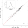 |
Fig. 1. Stellar masses estimated in this work for the galaxies in the low-z calibrating sample compared to those from the MPA/JHU catalogues. The red line represents a linear fit to the data, and the histogram of the residual of galaxies around the best-fit line is plotted in the inset. |
2.2. DEEP2 galaxy sample
The high-z galaxy sample used in this work is based on the third data release (Newman et al. 2013) of the DEEP2 survey and the Ks-band selected catalogue of Bundy et al. (2006). The DEEP2 Galaxy Redshift Survey (Davis et al. 2003) utilizes the DEIMOS spectrograph (Faber et al. 2003) on the Keck II telescope. Targets for the spectroscopic sample were selected from BRI photometry (Coil et al. 2004) taken with the 12k × 8k mosaic camera on the Canada-France-Hawaii Telescope (CFHT). The images have a limiting magnitude of RAB ∼ 25.5. Since the R-band provides the highest signal-to-noise ratio (S/N) among all the CFHT bands, the photometry in this band was used to select targets for spectroscopic observations with the DEEP2 spectrograph. The CFHT imaging covers four widely separated regions, with a total area of 3.5 deg2. In fields 2−4, the spectroscopic sample is pre-selected using (B − R) and (R − I) colours to eliminate objects with z < 0.7 (Davis et al. 2003). Colour and apparent magnitude cuts were also applied to objects in the first field, the Extended Groth Strip (EGS), but these were designed to down-weight low-redshift galaxies to select a roughly equal number of galaxies below and above z = 0.7 (Willmer et al. 2006).
Based on the DEEP2 sample, Bundy et al. (2006) conducted an extensive imaging survey of all the DEEP2 fields with the Wide Field Infrared Camera (WIRC; Wilson et al. 2003) on the 5 m Hale Telescope at Palomar Observatory. Using contiguously spaced pointings, the central third of fields 2−4 was mapped to a median 80% completeness depth greater than KAB = 21.5, accounting for 0.9 deg2 on the sky. The EGS field covers 0.7 deg2 with varying but deeper depths. A stellar mass was estimated by Bundy et al. (2006) for each of their galaxies. First, a Ks-band mass-to-light ratio M*/LKs was obtained by comparing the observed BRIKs SED to a grid of 13 440 synthetic SEDs constructed from BC03 and spanning a range of star formation histories, ages, metallicities, and dust contents. The stellar mass of the galaxy was then given by scaling M*/LKs to the Ks-band luminosity measured from the total Ks-band magnitude and the DEEP2 spectroscopically measured redshift.
In this work we make use of the galaxy sample from Bundy et al. (2006), which consists of 7222 galaxies with redshifts in the range 0.75 ≤ z ≤ 1.40, redshift quality parameters zquality ≥ 3, and Ks-band magnitudes Ks ≤ 20. For consistency, we estimated a stellar mass for each of the galaxies using the same method we used above for the low-z calibrating sample. The observed SED used for the estimation involves photometry in the B, R, I, and Ks bands. Our stellar mass estimates are compared in Fig. 2 to those obtained by Bundy et al. (2006); they are in good agreement with no obvious systematic difference. We also estimated the rest-frame g − i and NUV − r colours for the galaxies using the same method.
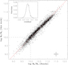 |
Fig. 2. Stellar masses estimated in this work for the DEEP2 galaxies compared to those from Bundy et al. (2006). The red line represents a linear fit to the data, and the histogram of the residual of galaxies around the best-fit line is plotted in the inset. Bundy et al. (2006) found that the spectroscopic sample in DEEP2 regions is incomplete below M* ∼ 1010 M⊙. |
Following previous studies (e.g., Bundy et al. 2006; Chen et al. 2009), we weighted each galaxy in our DEEP2 sample to correct for incompleteness when performing statistical analyses:
 (1)
(1)
where κ accounts for incompleteness resulting from the DEEP2 colour selection and redshift success rate. The ‘optimal’ weighting model of Willmer et al. (2006) was used to estimate κ, which accounts for the redshift success rate for red and blue galaxies in different ways. We adopted the luminosity-dependent colour divider employed by van Dokkum (2008) for classifying the galaxies into red and blue:
 (2)
(2)
where the rest-frame U − B colour and the B-band absolute magnitude MB are obtained above using our Bayesian approach. The U − B histogram and the MB versus U − B diagram are shown in Fig. 3 for two successive redshift intervals: 0.75 < z < 1 and 1 < z < 1.4.
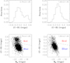 |
Fig. 3. Histograms of the rest-frame U − B colour (top panels) and diagrams of U − B vs. B-band absolute magnitude (lower panels) shown for DEEP2 galaxies in two successive redshift intervals: 0.75 < z < 1 (left-hand panels) and 1 < z < 1.4 (right-hand panels). The dashed line in the lower panels is the luminosity-dependent colour divider employed by van Dokkum (2008), which is used in this work to classify our galaxies into red and blue populations. Magnitudes plotted in this figure are in the Vega system. |
The second factor, Vmax, is defined as the maximum volume over which the galaxy would be included in the sample, accounting for the fact that faint galaxies are not detected throughout the entire survey volume in a flux-limited survey. Following Willmer et al. (2006), the  for a galaxy i can be calculated as:
 (3)
(3)
where z and Ω are the redshift and the solid angle, respectively. The redshift limits zmin, i and zmax, i are imposed either by the limits of the redshift bin being dealt with or by the apparent magnitude limits of the DEEP2 sample. More details can be found in Willmer et al. (2006).
We estimated stellar mass functions for the two redshift bins, which are plotted in Fig. 4 as diamonds connected by solid lines, and these are compared to the estimates obtained by Bundy et al. (2006), shown as crosses connected by dashed lines. The two estimates are almost identical, indicating that we have correctly calculated the weights for incompleteness correction. For the mass function estimates (and the HIMFs in the next section), we used 5372 out of the 7222 galaxies with M* > 1010 M⊙. Below this mass, the DEEP2 sample becomes significantly incomplete (Bundy et al. 2006). The errors on the stellar mass functions were estimated using the 1σ scatter in the measurements of the four DEEP2 fields.
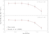 |
Fig. 4. Stellar mass functions at two redshift intervals, as indicated (plotted in black diamonds), compared to the measurements from Bundy et al. (2006; plotted in red crosses). |
For one of the four DEEP2 fields (the EGS), the SFR measurements of galaxies were carried out by Barro et al. (2011) using SEDs covering the wavebands from UV to far-infrared, including the IRAC 3.5 and 4.6 μm bands. Around 2000 blue galaxies in the EGS field in our sample have SFRs measured in this way.
3. Results
3.1. The H I mass fraction estimator
The H I-to-stellar mass ratio is strongly correlated with galaxy parameters such as optical colours, NUV − r colour, μ*, R90/R50, and M*, with a typical scatter of ∼0.35 dex. The relation between MHI/M* and the combination of two or more parameters is tighter than the relation between MHI/M* and a single parameter, with a typical scatter of ∼0.30 dex (Zhang et al. 2009; Li et al. 2012; Catinella et al. 2010). Unlike Zhang et al. (2009), we took the combination of NUV − r and μ*, instead of optical colour and μ*, in this work because of two considerations. First, as we see from Fig. 5, low-redshift galaxies show a very narrow dynamic range in g − i, with 1 ≲ g − i ≲ 1.2, but NUV − r spans a broader range of values (3.5 ≲ (NUV − r) ≲ 6). This is more clearly seen in the right-hand panel of the same figure, where g − i is plotted against NUV − r. When NUV − r increases above ∼3.5, g − i does not increase any more and is fairly constant at g − i ≈ 1.1, suggesting that NUV − r is more sensitive than g − i to the atomic gas content for the most H I-poor galaxies. This is consistent with the finding of Catinella et al. (2010) that, among the four parameters considered (M*, μ*, R90/R50, NUV − r), the NUV − r colour was the one most tightly correlated with the H I-to-stellar mass ratio. Second, for the DEEP2 galaxies at z ∼ 1, their rest-frame NUV magnitude is red-shifted to the optical band, and in this case the k-correction is relatively small and can be estimated more reliably than in the case where the g magnitude is used.
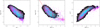 |
Fig. 5. Correlation of the H I-to-stellar mass ratio (MHI/M*) with g − i (left) and NUV − r (middle) for the low-z calibrating sample. The best-fit models are plotted as solid red lines (see the text for a detailed description). Right-hand panel: relation between g − i and NUV − r for the same set of galaxies. The low-z calibrating sample is plotted as cyan dots, the RESOLVE sample is plotted as magenta crosses, and the final ALFALFA 100% catalogue (α.100) is shown as black-and-white contours in each panel. |
The physical reason why H I is better predicted by NUV − r colour likely arises from the fact that the UV emission from a galaxy traces the light from young stars in the low-density extended gas in the outer disks of galaxies that has not been absorbed by dust. The molecular gas traced by CO emission is, on the other hand, known to be tightly correlated with the infrared luminosity of the galaxy (Young et al. 1984; Sanders & Mirabel 1985). This analysis will not address the molecular content of the galaxies in our sample.
We checked the results of the low-z calibrating sample using more recent data from two larger H I catalogues. The first is the REsolved Spectroscopy of a Local VolumE (RESOLVE2) sample, which is completed in baryonic mass (defined as Mbary = M* + 1.4 MHI) down to dwarfs of ∼109 M⊙ (Eckert et al. 2015; Stark 2016). The second is the final ALFALFA 100% catalogue (α.1003) (Jones et al. 2018; Haynes et al. 2018). The galaxies with S/Ns lower than five are excluded from this sample. The RESOLVE and the α.100 samples are shown in Fig. 5 as magenta crosses and black-and-white contours, respectively. We note that the colours and the stellar masses used for these two samples were obtained from the NASA-Sloan Atlas (NSA) catalogue (v1_0_14) and that the colours were corrected for Galactic extinction. As a result, around 1500 RESOLVE galaxies and around 13 000 α.100 galaxies were used in the comparison with the low-z calibrating sample. We can see that the low-z calibrating sample, though small, follows the same trend with the RESOLVE and α.100 samples. This confirms that the estimator derived using the low-z calibrating sample is robust.
We used a polynomial function to represent the observed non-linear relation of MHI/M* versus NUV − r,
 (4)
(4)
plotted as a red line in the middle panel of Fig. 5. Here the best-fit parameters are a0 = 2.26432, a1 = −1.46308, a2 = 0.202311, and a3 = −0.0108242. The 1σ scatter of the galaxies around this relation is 0.36 dex.
We explored possible systematic effects due to dust attenuation on the correlation between the H I gas fraction and NUV − r colour. An Hα-to-Hβ decrement can be used as an indicator of dust attenuation: Higher values of Hα/Hβ indicate higher dust attenuation values. We obtained a sample of ∼10 000 galaxies (hereafter the α.100_spec sample) that have high signal-to-noise detection of Hα and Hβ emission lines (S/N > 3) by cross-matching the α.100 sample with the SDSS eighth data release spectroscopic sample. We note that all galaxies on the star-forming main sequence in SDSS have Hα and Hβ with this S/N or higher. We divided the sample into three sub-samples according to the Hα-to-Hβ ratio as shown in the top-left panel of Fig. 6, and we plot these sub-samples in the H I gas fraction and NUV − r colour diagram in the other three panels. As in the middle panel of Fig. 5, the final ALFALFA 100% catalogue (α.100) is shown as black-and-white contours for comparison. The galaxies that have Hα and Hβ detections are over-plotted as green dots, with the cuts noted on the top of each panel. The solid red line is the relation described in Eq. (4). It is found that the galaxies with higher dust attenuation have redder NUV − r colours and lower H I gas fractions. However, they still follow the correlation between the H I gas fraction and NUV − r colour. We conclude that it is safe to apply the estimator to galaxies with varying dust attenuation values.
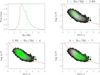 |
Fig. 6. Effect of dust attenuation on the relation between MHI/M* and NUV − r colour. The distribution of the Hα-to-Hβ ratio of the α.100_spec sample is shown in the top-left panel. The dashed green lines indicate the division of the sample into three sub-samples. In the other panels, the three sub-samples are shown as green dots in the MHI/M* vs. NUV − r diagram. Similar to the middle panel in Fig. 5, the black-and-white contours represent the final ALFALFA 100% catalogue (α.100), while the solid red line is the relation described in Eq. (4). As can be seen, galaxies of different dust contents are shifted along the derived relation, not displaced away from it. |
Figure 7 shows the relationship between the H I-to-stellar mass ratio (G/S) and a linear combination of NUV − r and stellar surface mass density μ*, defined as 0.5  – where M* is the stellar mass of the galaxy and R50 is its z-band half-light radius in units of kpc – for the galaxies in the low-z calibrating sample. This estimator could in theory be expected to exhibit less scatter than one based on NUV − r colour alone if the surface density of the atomic gas is well correlated with the surface density of the stars in galaxies. In practice, however, the H I often extends far beyond the disk traced in the optical light. Wang et al. (2013) show that there is a factor of ∼1.5 scatter in the ratio between H I size and optical size at a fixed stellar mass, implying a factor of two or more scatter in surface density. We find that the estimator that includes μ* has a scatter around the one-to-one line of 0.30 dex. We can obtain somewhat tighter results if we fit separate relations for galaxies with (NUV − r) > 3.5 and (NUV − r) < 3.5. The scatter of blue and red galaxies around their separate relations is 0.27 and 0.36 dex, respectively. The higher scatter for redder galaxies is likely due to the fact that these galaxies contain more dust and a higher fraction of their total gas content is in molecular rather than atomic form.
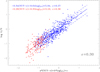 |
Fig. 7. Relation between the H I gas fraction and the linear combination of NUV − r colour and stellar surface mass density (μ*) in the SDSS-z band. The low-z calibrating sample has been divided into two sub-samples according to NUV − r colour: The red points are galaxies with (NUV − r) > 3.5, and the blue points are galaxies with (NUV − r) < 3.5. The fitting parameters are labelled at the top left of the figure. |
This estimator cannot be applied to all the high-z samples directly because only one of the four DEEP2 fields, the EGS region, has a half-light radius determined for each galaxy from Hubble Space Telescope (HST) observations. Before we applied the estimator to the EGS galaxies, we noticed that the HST half-light radius is determined in the I-band with an effective wavelength of 8140 Å, corresponding to a rest-frame wavelength ranging from 3391 Å to 4651 Å for our galaxies. However, the μ* for the low-z calibrating sample was obtained from the SDSS z-band at 8931 Å. As shown in Fig. 8, the surface mass density μ* of galaxies changes from band to band due to the wavelength dependence of their half-light radii. In order to take this effect into account, we used the median difference in log μ* shown in the figure, to make a correction to μ* for galaxies in the EGS. Then we compared the gas fractions estimated for these galaxies from the linear combination of NUV − r and μ* with the gas fractions given by NUV − r only, finding systematic differences that depend on redshift, as shown in Fig. 9. For red and blue galaxies, the gas fraction that takes μ* into account is smaller by 0−0.1 and 0.2−0.5 dex, respectively.
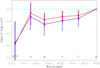 |
Fig. 8. Difference between μ* in the GALEX-NUV and SDSS-u, g, r, i bands compared to that in the SDSS-z band. As in Fig. 7, the red and blue colours represent galaxies with (NUV − r) > 3.5 and (NUV − r) < 3.5, respectively. |
In summary, we have demonstrated in this section that, among the quantities we have access to, the combination of NUV − r colour and stellar surface density yields the best predictor for the H I mass fraction for blue galaxies in particular. Use of a single colour such as NUV − r leads to inaccurate predictions that depend on the weighting between the red and blue galaxies in the sample. We show that a separate calibration for the two populations is necessary to obtain accurate estimates of the high-mass end of the HIMF and the cosmic H I mass density. In this analysis, we applied the median difference, shown with the red and blue stars and lines in Fig. 9, to correct the gas fraction for all the galaxies in our DEEP2 sample. We note that our analysis in the following sections does not include any estimate of the molecular gas content of the galaxies and that this component may have very different scaling relations than those of the atomic gas.
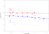 |
Fig. 9. Difference between the G/S estimated from NUV − r and μ* and the G/S estimated from NUV − r only as a function of redshift. The median value in each redshift bin and the linear fitting results of these median values are shown as stars and solid lines, respectively. The contours enclose 34, 68, and 90% of the sample. Similar to Fig. 7, the red and blue colours represent galaxies with (NUV − r) > 3.5 and (NUV − r) < 3.5, respectively. |
3.2. H I mass function at z ∼1
Applying the H I mass fraction estimator obtained above, we estimated an H I gas mass for each of the galaxies in the DEEP2 sample. The first statistic that we obtained from these data is the HIMF, which quantifies the co-moving number density of galaxies as a function of their H I mass. This statistic had not previously been estimated at these high redshifts. Specifically, we estimated the HIMF for two successive redshift intervals, one below and one above z = 1. These are shown in Fig. 10 as solid black circles connected by a solid line. When estimating the HIMFs, we corrected for sample incompleteness in the same way as described above for estimating the stellar mass functions. We restricted ourselves to galaxies with log(M*/M⊙) > 10 for the same reason explained above. The errors on the HIMFs are estimated from the 1σ scatter of the HIMFs of the four separate DEEP2 fields.
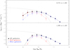 |
Fig. 10. H I mass functions estimated from DEEP2 for the two indicated redshift intervals plotted with solid black circles connected by a solid line for the whole sample, and in red (blue) diamonds connected by a dashed line for the red (blue) galaxy sub-samples. For comparison, the HIMF at z = 0 from α.100 is shown as solid grey lines. |
For each redshift interval we also estimated an HIMF for the subset of galaxies with either red or blue U − B colours, classified using the colour divider in Eq. (2). The estimates are also shown in Fig. 10. For comparison, the HIMF of the local Universe obtained by Jones et al. (2018) from the final catalogue of the ALFALFA (α.100) is plotted as a solid grey line in the same figure.
We see that at H I masses above ∼1010 M⊙, the abundance of galaxies decreases slowly with increasing H I mass before it drops rapidly at masses above ∼1011 M⊙. This behaviour is similar to the luminosity functions and stellar mass functions found in the local Universe, which can usually be described by a Schechter function. At masses below ∼1010 M⊙, the HIMFs also decrease, and this can be attributed to the fact that the galaxies with stellar masses below 1010 M⊙ are not included in the measurement. For this reason, the HIMFs presented here can only be regarded as lower limits of the number density of galaxies with H I masses lower than ∼1010 M⊙. Therefore, in the following analysis we only fit a Schechter function to the HIMFs at H I masses above 1010 M⊙.
We note that the errors on the H I masses can affect the shape of the HIMFs, in particular at the high-mass end. Given that the scatter in our estimates of the gas fraction log(MHI/M*) and in the stellar mass log(M*) are 0.30 dex (see Fig. 2) and 0.11 dex (see Fig. 7), respectively, the scatter of H I gas mass log(MHI) is estimated as 0.32 dex. Considering the uncertainties of the corrections described in Sect. 3.1, a total error in log(MHI) of 0.35 dex is assumed. We then fitted a Schechter function to the HIMFs at H I masses above 1010 M⊙ by considering the scatter of log(MHI) to have a value of 0.35 dex. We note that the flat slope of the HIMF at low masses is highly uncertain because of the extrapolation to low masses. We tried to fit to the HIMF measurements with the slope parameter fixed to three different values, α = −1, −1.5, and −2, and plot the best-fit functions as dashed red, cyan, and magenta lines in Fig. 11. As can be seen from the figure, fitting different Schechter function slopes to the HIMFs cannot effectively constrain the slope parameter at the low-mass end. At the high-mass end, the shape is well constrained and consistent with no evolution at the bright end.
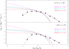 |
Fig. 11. Schechter function fits with the slope fixed to α = −2, −1.5, and −1.0 shown as dashed magenta, cyan, and red lines, respectively. During fitting, a 0.35 dex scatter of log(MHI) is adopted. The corresponding Schechter functions without scatter in log(MHI) are shown as solid lines. |
3.3. H I mass density at z ∼1
The second quantity that we obtained from our data is the cosmic H I mass density, ΩHI, which is the volume density of the H I mass contained in galaxies at a given redshift normalized by the critical density of matter in the Universe. Because of large uncertainties for the slope at the low-mass end, we did not try to estimate the total ΩHI from the best-fit Schechter functions shown in Fig. 11. Instead, we measured the lower limits of ΩHI by directly integrating the HIMFs, using galaxies with M* > 1010 M⊙. The scatter among the four DEEP2 fields was adopted as the 1σ uncertainty on the measurement. We derived lower limits ΩHI, limit
 and
and  for the two redshift bins. We note that the mean measurement of
  at z ∼ 1 is comparable with that of
  if 21 cm signatures of blue star-forming galaxies with MB ≤ −20 at similar redshifts in the DEEP2 fields are directly stacked (Chowdhury et al. 2020).
3.4. Correlations between H I mass fraction, stellar mass, specific star formation rate, and H I depletion time
In this subsection we study the correlation of the H I gas content of the galaxies at z ∼ 1 with their SFR using galaxies from the EGS, for which SFR measurements of galaxies are available. The SFR measurements range from 1 to 3 M⊙ yr−1, with a median value of 1.2 M⊙ yr−1. In Figs. 12 and 13 we use this sample (again, split into two sub-samples by redshift), as well as the low-z calibrating sample, to examine the correlations between the sSFR, the H I mass fraction, and the quantity MHI/SFR. We note that MHI/SFR should be regarded as a lower limit to the actual time taken for the H I gas to be depleted. In low-redshift galaxies, most of the H I gas is often well outside the star-forming disk in a dynamically stable configuration. Some of this gas may be a reservoir for future star formation in the galaxy, but the timescale for the consumption of the gas will depend on uncertain parameters, such as gas inflow rates. At high redshifts, gas inflow rates are higher, the dynamical timescales of galaxies are shorter, and extended gas reservoirs may be converted into stars more quickly. Therefore, one might expect to see a better correlation between the SFR and the H I gas content at high redshift. Our results, however, indicate that this is not true.
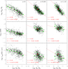 |
Fig. 12. H I-to-stellar mass ratio (MHI/M*; top panels), sSFR (SFR/M*; second row of panels), and H I gas depletion time (MHI/SFR; bottom panels) plotted as a function of stellar mass, for the low-z calibrating sample (left) and the DEEP2 galaxies at the two higher redshifts (centre and right-hand panels). The small black dots are for the low-z calibrating sample or the blue galaxies at high redshifts, and the red line in each panel shows the best fitting with a linear relation. The stars and the two solid lines plotted in green show the median and 1σ scatter for a number of stellar mass bins, respectively. For comparison, the mean measurements of star-forming galaxies at redshift z ∼ 1 by Chowdhury et al. (2020) are plotted as filled red circles. |
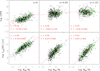 |
Fig. 13. Correlations of sSFRs and H I gas depletion times with the H I-to-stellar mass ratio plotted for the same sets of galaxies with the same symbols and lines as in the previous figure. |
The top three panels in Fig. 12 show the distribution of galaxies in the log MHI/M* versus log M* plane. The low-z calibrating sample shows a tight, nearly linear relation with a slope of −0.54 and a 1σ scatter of 0.38 dex. A similarly tight relation is seen at z = 0.83 and z = 1.23, with a scatter of 0.31 and 0.35 dex. The correlation seems to steepen at higher redshifts; fitting a linear relation to the data leads to slope parameters of −0.82 and −1.04 for the two high-z samples, compared to −0.54 for the low-z sample. To take the effect of incompleteness into account, we also fitted the data weighted by 1/Vmax. The resulting slopes are −0.72 and −0.93. The normalization of the correlation also increases with redshift. At a stellar mass of 1011 M⊙, the average H I-to-stellar mass ratio at z ∼ 0 is 0.1, and this increases by a factor of 3−4, up to ∼0.3 at z ∼ 0.8 and ∼0.4 at z ∼ 1.2. The increase is even more dramatic at smaller stellar masses, for example by a factor of 4−12 at M* = 1010 M⊙. These results show that distant galaxies are on average much more H I-rich than local galaxies and that the slope of the relation between the H I gas mass fraction and stellar mass also evolves with redshift. We checked the nature of the galaxies with MHI > 1010 M⊙ in the EGS field and find that their half-light radii in the HST I-band vary from 20 to 90 kpc and that the surface mass density of H I gas using this size estimate is about 37 M⊙ pc−2.
In the middle panels of Fig. 12, we reproduce the star formation sequence by showing the log(SFR/M*) versus log M* planes. There is a similar increase in the normalization of the relation. Interestingly, the relation between the sSFR and stellar mass shows larger scatter at z ∼ 1 than the relation between the H I gas mass fraction and stellar mass. We note that the molecular gas fraction also increases by a factor of 3−4, from z = 0 to z ∼ 0.8 and z ∼ 1.2, according to the evolution trend of fmol − gas ∝ (1 + z)2 (Geach et al. 2011; Carilli & Walter 2013).
In the bottom panels of Fig. 12, we show the correlation of MHI/SFR with stellar mass for the same sets of galaxies. This quantity yields rather short timescales at all redshifts probed (0.5−2 Gyr at z ∼ 1 and a factor of only ∼2 larger at z ∼ 0), but, as we have noted, these are likely lower limits to the actual time taken for the gas to be consumed. What is more interesting is that this quantity exhibits very weak redshift evolution, similar to the H I gas and star formation main sequences discussed above. This indicates that the star formation main sequence may simply be a natural result of the cosmic evolution of the available gas reservoir in galaxies. Furthermore, it is also seen that MHI/SFR at a fixed stellar mass shows a huge scatter, ∼0.6 dex at z ∼ 1 and ∼0.4 dex in the local Universe, implying a weak correlation between MHI and SFR, as expected for a gas component that is not directly linked with the star formation in the galaxy population.
In the upper panels of Fig. 13 we plot the galaxies in the plane of log(SFR/M*) versus MHI/M*. At z ∼ 1 the sSFR is confined to a narrow range, again reflecting the tightness of the star formation sequence, while MHI/M* spans a much wider range. This causes the quantity MHI/SFR to be tightly correlated with MHI/M*, as shown in the lower panels of the figure.
The scaling relations shown in Figs. 13 and 14 are best interpreted in conjunction with either semi-analytic models of galaxy formation that model the spatial distribution of the gas (e.g., Fu et al. 2010; Lagos et al. 2011; Popping et al. 2014; Xie et al. 2017) or cosmological hydrodynamical simulations with sufficient resolution (1 kpc or better) to resolve the formation of galaxy disks over the same mass scales as in our sample (e.g., Vogelsberger et al. 2014; Schaye et al. 2015; Pillepich et al. 2018). These models follow the cooling and condensation of gas in galaxy halos. The formation of molecular gas is often incorporated as a post-processing step (e.g., Diemer et al. 2019). Comparisons with H I scaling relations, such as those presented in this section, then constrain gas accretion and condensation processes in the models, which depend sensitively on processes such as supernova and active galactic nucleus feedback.
4. Conclusions
Using the rest-frame NUV-optical colour, NUV − r, as a proxy for the H I-to-stellar mass ratio, MHI/M*, we have estimated the H I gas mass for a sample of ∼7000 galaxies in the DEEP2 survey with redshifts in the range 0.75 < z < 1.4 and stellar masses above ∼1010 M⊙. The correlation between MHI/M* and NUV − r is calibrated with a sample of 660 galaxies in the local Universe that have optical and NUV photometry from SDSS and GALEX, as well as 21 cm emission data from HyperLeda. With these H I mass estimates, we have calculated HIMFs and cosmic H I gas densities (ΩHI), and we have investigated the correlations between the sSFR (SFR/M*), the H I-to-stellar mass ratio (MHI/M*), and the H I gas depletion time (tdep(HI) ≡ MHI/SFR).
Our main conclusions can be summarized as follows.
-
For galaxies with stellar masses above ∼1010 M⊙, the HIMF at z ∼ 1 is quite similar to the local HIMF, while the low-mass end slope cannot be constrained due to the lack of low stellar mass galaxies in our sample.
-
Integrals of our HIMFs suggest the lower limit of the H I mass density at z ∼ 1 to be
 , which is significantly smaller than the estimates obtained by other authors based on DLAs at the same redshift. However, our work confirms the result of Kanekar et al. (2016), that massive star-forming galaxies do not dominate the neutral gas at z ∼ 1.
 -
Galaxies with M* ∼ 1011 M⊙ at z = 1 have large H I gas fractions, which are about 3−4 times higher than those of local galaxies, indicating that the neutral gas fraction evolves from z = 1 to the present epoch. It is found that the slope of the correlation between the H I gas fraction and stellar mass also has a modest evolution with redshift.
-
The quantity MHI/SFR exhibits very large scatter, and the scatter increases from a factor of 5−7 at z = 0 to factors close to 100 at z = 1. This implies that there is no relation between H I gas and star formation in high-redshift galaxies. The H I gas must be linked to cosmological gas accretion processes.
As discussed previously, all the results obtained in this work rely on the assumption that the same scaling relation between the H I mass fraction and NUV-optical colour applies at higher redshifts. Although our measurements of gas fractions and cosmic H I mass densities are consistent with those derived from the co-adding method or Mg II absorbers, it would be very useful to obtain small samples of galaxies with H I measured at z = 1 to verify that the scaling relations hold at this redshift. This goal should be achievable with the help of future radio telescopes such as the next-generation Very Large Array (ngVLA) and the Square Kilometre Array (SKA). From the linear fitting relations between MHI/M* and M* for the galaxies in two high-z bins in Fig. 12, a lower limit of MHI ∼ 2.7 × 10¹⁰ M⊙ is required to derive the scaling relations that cover a wide range of M*, from 109 to 1011 M⊙, at z ∼ 1. Using the equation  , where DMpc is the distance to the galaxy in Mpc, the integrated flux density detection threshold S21, th can be calculated as 2.6 × 10⁻³ Jy km s−1. Taking this threshold, a sufficient number of galaxies can be detected at z ∼ 1 according to the simulations of SKA detection rates (Obreschkow et al. 2009).
Acknowledgments
W.Z. is grateful to MPA for hospitality when this work was being completed. W.Z. deeply appreciates that Cheng Li has given a lot of guidance and recommendations for this work. W.Z. thanks Kevin Bundy for kindly sharing the catalogue of Ks magnitude and stellar mass. W.Z. thanks Zheng Zheng, and Qi Guo for helpful suggestions. This work is supported by the Joint Research Fund in Astronomy (No. U1531118) under cooperative agreement between the National Natural Science Foundation of China (NSFC) and Chinese Academy of Sciences (CAS). This work is also sponsored by NSFC (No. 12090041, 12090040, 10903011, 11173045, 11733006), the National Key R&D Program of China grant No. 2017YFA0402704, and the Guangxi Natural Science Foundation (No. 2019GXNSFFA245008). J.F. acknowledges the support by the Youth innovation Promotion Association CAS and Shanghai Committee of Science and Technology grant No. 19ZR1466700 and the support by the Joint Research Fund in Astronomy (No. U1531123). This work has made use of data from the SDSS and SDSS-II, and the HyperLeda database.
References
- Barro, G., Pérez-González, P. G., Gallego, J., et al. 2011, ApJS, 193, 30 [NASA ADS] [CrossRef] [Google Scholar]
- Bruzual, G., & Charlot, S. 2003, MNRAS, 344, 1000 [NASA ADS] [CrossRef] [Google Scholar]
- Bundy, K., Ellis, R. S., Conselice, C. J., et al. 2006, ApJ, 651, 120 [NASA ADS] [CrossRef] [Google Scholar]
- Cardelli, J. A., Clayton, G. C., & Mathis, J. S. 1989, ApJ, 345, 245 [NASA ADS] [CrossRef] [Google Scholar]
- Carilli, C. L., & Walter, F. 2013, ARA&A, 51, 105 [Google Scholar]
- Catinella, B., Haynes, M. P., Giovanelli, R., Gardner, J. P., & Connolly, A. J. 2008, ApJ, 685, L13 [NASA ADS] [CrossRef] [Google Scholar]
- Catinella, B., Schiminovich, D., Kauffmann, G., et al. 2010, MNRAS, 403, 683 [NASA ADS] [CrossRef] [Google Scholar]
- Catinella, B., Saintonge, A., Janowiecki, S., et al. 2018, MNRAS, 476, 875 [NASA ADS] [CrossRef] [Google Scholar]
- Chang, T.-C., Pen, U.-L., Bandura, K., & Peterson, J. B. 2010, Nature, 466, 463 [NASA ADS] [CrossRef] [Google Scholar]
- Chen, Y.-M., Wild, V., Kauffmann, G., et al. 2009, MNRAS, 393, 406 [Google Scholar]
- Chowdhury, A., Kanekar, N., Chengalur, J. N., Sethi, S., & Dwarakanath, K. S. 2020, Nature, 586, 369 [Google Scholar]
- Coil, A. L., Newman, J. A., Kaiser, N., et al. 2004, ApJ, 617, 765 [NASA ADS] [CrossRef] [Google Scholar]
- Crighton, N. H. M., Murphy, M. T., Prochaska, J. X., et al. 2015, MNRAS, 452, 217 [NASA ADS] [CrossRef] [Google Scholar]
- Davis, M., Faber, S. M., Newman, J., et al. 2003, in Society of Photo-Optical Instrumentation Engineers (SPIE) Conference Series, ed. P. Guhathakurta, 4834, 161 [Google Scholar]
- Decarli, R., Aravena, M., Boogaard, L., et al. 2020, ApJ, 902, 110 [Google Scholar]
- Diemer, B., Stevens, A. R. H., Lagos, C. D. P., et al. 2019, MNRAS, 487, 1529 [NASA ADS] [CrossRef] [Google Scholar]
- Eckert, K. D., Kannappan, S. J., Stark, D. V., et al. 2015, ApJ, 810, 166 [CrossRef] [Google Scholar]
- Faber, S. M., Phillips, A. C., Kibrick, R. I., et al. 2003, in SPIE Conf. Ser., eds. M. Iye, & A. F. M. Moorwood, 4841, 1657 [Google Scholar]
- Fernández, X., Gim, H. B., van Gorkom, J. H., et al. 2016, ApJ, 824, L1 [NASA ADS] [CrossRef] [Google Scholar]
- Fu, J., Guo, Q., Kauffmann, G., & Krumholz, M. R. 2010, MNRAS, 409, 515 [NASA ADS] [CrossRef] [Google Scholar]
- Geach, J. E., Smail, I., Moran, S. M., et al. 2011, ApJ, 730, L19 [Google Scholar]
- Giovanelli, R., Haynes, M. P., Kent, B. R., et al. 2005, AJ, 130, 2598 [NASA ADS] [CrossRef] [Google Scholar]
- Haynes, M. P., Giovanelli, R., Kent, B. R., et al. 2018, ApJ, 861, 49 [Google Scholar]
- Jones, M. G., Haynes, M. P., Giovanelli, R., & Moorman, C. 2018, MNRAS, 477, 2 [NASA ADS] [CrossRef] [Google Scholar]
- Kanekar, N., Sethi, S., & Dwarakanath, K. S. 2016, ApJ, 818, L28 [CrossRef] [Google Scholar]
- Kannappan, S. J. 2004, ApJ, 611, L89 [NASA ADS] [CrossRef] [MathSciNet] [Google Scholar]
- Kauffmann, G., Heckman, T. M., White, S. D. M., et al. 2003, MNRAS, 341, 33 [NASA ADS] [CrossRef] [Google Scholar]
- Kauffmann, G., Li, C., Zhang, W., & Weinmann, S. 2013, MNRAS, 430, 1447 [NASA ADS] [CrossRef] [Google Scholar]
- Kroupa, P. 2001, MNRAS, 322, 231 [NASA ADS] [CrossRef] [Google Scholar]
- Lagos, C. D. P., Lacey, C. G., Baugh, C. M., Bower, R. G., & Benson, A. J. 2011, MNRAS, 416, 1566 [NASA ADS] [CrossRef] [Google Scholar]
- Lah, P., Chengalur, J. N., Briggs, F. H., et al. 2007, MNRAS, 376, 1357 [NASA ADS] [CrossRef] [Google Scholar]
- Lah, P., Pracy, M. B., Chengalur, J. N., et al. 2009, MNRAS, 399, 1447 [NASA ADS] [CrossRef] [Google Scholar]
- Li, C., Kauffmann, G., Fu, J., et al. 2012, MNRAS, 424, 1471 [CrossRef] [Google Scholar]
- Martin, D. C., Fanson, J., Schiminovich, D., et al. 2005, ApJ, 619, L1 [Google Scholar]
- Masui, K. W., Switzer, E. R., Banavar, N., et al. 2013, ApJ, 763, L20 [CrossRef] [Google Scholar]
- Meyer, M. J., Zwaan, M. A., Webster, R. L., et al. 2004, MNRAS, 350, 1195 [NASA ADS] [CrossRef] [Google Scholar]
- Neeleman, M., Prochaska, J. X., Ribaudo, J., et al. 2016, ApJ, 818, 113 [NASA ADS] [CrossRef] [Google Scholar]
- Newman, J. A., Cooper, M. C., Davis, M., et al. 2013, ApJS, 208, 5 [Google Scholar]
- Noeske, K. G., Weiner, B. J., Faber, S. M., et al. 2007, ApJ, 660, L43 [Google Scholar]
- Noterdaeme, P., Petitjean, P., Carithers, W. C., et al. 2012, A&A, 547, L1 [NASA ADS] [CrossRef] [EDP Sciences] [Google Scholar]
- Obreschkow, D., Klöckner, H. R., Heywood, I., Levrier, F., & Rawlings, S. 2009, ApJ, 703, 1890 [NASA ADS] [CrossRef] [Google Scholar]
- Paturel, G., Theureau, G., Bottinelli, L., et al. 2003, A&A, 412, 57 [NASA ADS] [CrossRef] [EDP Sciences] [Google Scholar]
- Pen, U.-L., Staveley-Smith, L., Peterson, J. B., & Chang, T.-C. 2009, MNRAS, 394, L6 [NASA ADS] [Google Scholar]
- Pillepich, A., Springel, V., Nelson, D., et al. 2018, MNRAS, 473, 4077 [Google Scholar]
- Popping, G., Somerville, R. S., & Trager, S. C. 2014, MNRAS, 442, 2398 [Google Scholar]
- Prochaska, J. X., & Wolfe, A. M. 2009, ApJ, 696, 1543 [NASA ADS] [CrossRef] [Google Scholar]
- Rao, S. M., Turnshek, D. A., & Nestor, D. B. 2006, ApJ, 636, 610 [NASA ADS] [CrossRef] [Google Scholar]
- Rao, S. M., Turnshek, D. A., Sardane, G. M., & Monier, E. M. 2017, MNRAS, 471, 3428 [NASA ADS] [CrossRef] [Google Scholar]
- Salim, S., Charlot, S., Rich, R. M., et al. 2005, ApJ, 619, L39 [Google Scholar]
- Sánchez-Ramírez, R., Ellison, S. L., Prochaska, J. X., et al. 2016, MNRAS, 456, 4488 [NASA ADS] [CrossRef] [Google Scholar]
- Sanders, D. B., & Mirabel, I. F. 1985, ApJ, 298, L31 [NASA ADS] [CrossRef] [Google Scholar]
- Schaye, J., Crain, R. A., Bower, R. G., et al. 2015, MNRAS, 446, 521 [Google Scholar]
- Schlegel, D. J., Finkbeiner, D. P., & Davis, M. 1998, ApJ, 500, 525 [NASA ADS] [CrossRef] [Google Scholar]
- Stark, D. P. 2016, ARA&A, 54, 761 [Google Scholar]
- van Dokkum, P. G. 2008, ApJ, 674, 29 [NASA ADS] [CrossRef] [Google Scholar]
- Vogelsberger, M., Genel, S., Springel, V., et al. 2014, MNRAS, 444, 1518 [NASA ADS] [CrossRef] [Google Scholar]
- Walter, F., Carilli, C., Neeleman, M., et al. 2020, ApJ, 902, 111 [Google Scholar]
- Wang, J., Overzier, R., Kauffmann, G., von der Linden, A., & Kong, X. 2010, MNRAS, 401, 433 [NASA ADS] [CrossRef] [Google Scholar]
- Wang, J., Kauffmann, G., Overzier, R., et al. 2011, MNRAS, 412, 1081 [Google Scholar]
- Wang, J., Kauffmann, G., Józsa, G. I. G., et al. 2013, MNRAS, 433, 270 [NASA ADS] [CrossRef] [Google Scholar]
- Willmer, C. N. A., Faber, S. M., Koo, D. C., et al. 2006, ApJ, 647, 853 [NASA ADS] [CrossRef] [Google Scholar]
- Wilson, J. C., Eikenberry, S. S., Henderson, C. P., et al. 2003, in SPIE Conf. Ser., eds. M. Iye, & A. F. M. Moorwood, 4841, 451 [Google Scholar]
- Wyder, T. K., Martin, D. C., Schiminovich, D., et al. 2007, ApJS, 173, 293 [NASA ADS] [CrossRef] [Google Scholar]
- Xie, L., De Lucia, G., Hirschmann, M., Fontanot, F., & Zoldan, A. 2017, MNRAS, 469, 968 [Google Scholar]
- Young, J. S., Kenney, J., Lord, S. D., & Schloerb, F. P. 1984, ApJ, 287, L65 [NASA ADS] [CrossRef] [Google Scholar]
- Zafar, T., Péroux, C., Popping, A., et al. 2013, A&A, 556, A141 [NASA ADS] [CrossRef] [EDP Sciences] [Google Scholar]
- Zhang, W., Li, C., Kauffmann, G., et al. 2009, MNRAS, 397, 1243 [NASA ADS] [CrossRef] [Google Scholar]
- Zhang, W., Li, C., Kauffmann, G., & Xiao, T. 2013, MNRAS, 429, 2191 [Google Scholar]
All Figures
|
Fig. 1. Stellar masses estimated in this work for the galaxies in the low-z calibrating sample compared to those from the MPA/JHU catalogues. The red line represents a linear fit to the data, and the histogram of the residual of galaxies around the best-fit line is plotted in the inset. |
| In the text | |
|
Fig. 2. Stellar masses estimated in this work for the DEEP2 galaxies compared to those from Bundy et al. (2006). The red line represents a linear fit to the data, and the histogram of the residual of galaxies around the best-fit line is plotted in the inset. Bundy et al. (2006) found that the spectroscopic sample in DEEP2 regions is incomplete below M* ∼ 1010 M⊙. |
| In the text | |
|
Fig. 3. Histograms of the rest-frame U − B colour (top panels) and diagrams of U − B vs. B-band absolute magnitude (lower panels) shown for DEEP2 galaxies in two successive redshift intervals: 0.75 < z < 1 (left-hand panels) and 1 < z < 1.4 (right-hand panels). The dashed line in the lower panels is the luminosity-dependent colour divider employed by van Dokkum (2008), which is used in this work to classify our galaxies into red and blue populations. Magnitudes plotted in this figure are in the Vega system. |
| In the text | |
|
Fig. 4. Stellar mass functions at two redshift intervals, as indicated (plotted in black diamonds), compared to the measurements from Bundy et al. (2006; plotted in red crosses). |
| In the text | |
|
Fig. 5. Correlation of the H I-to-stellar mass ratio (MHI/M*) with g − i (left) and NUV − r (middle) for the low-z calibrating sample. The best-fit models are plotted as solid red lines (see the text for a detailed description). Right-hand panel: relation between g − i and NUV − r for the same set of galaxies. The low-z calibrating sample is plotted as cyan dots, the RESOLVE sample is plotted as magenta crosses, and the final ALFALFA 100% catalogue (α.100) is shown as black-and-white contours in each panel. |
| In the text | |
|
Fig. 6. Effect of dust attenuation on the relation between MHI/M* and NUV − r colour. The distribution of the Hα-to-Hβ ratio of the α.100_spec sample is shown in the top-left panel. The dashed green lines indicate the division of the sample into three sub-samples. In the other panels, the three sub-samples are shown as green dots in the MHI/M* vs. NUV − r diagram. Similar to the middle panel in Fig. 5, the black-and-white contours represent the final ALFALFA 100% catalogue (α.100), while the solid red line is the relation described in Eq. (4). As can be seen, galaxies of different dust contents are shifted along the derived relation, not displaced away from it. |
| In the text | |
|
Fig. 7. Relation between the H I gas fraction and the linear combination of NUV − r colour and stellar surface mass density (μ*) in the SDSS-z band. The low-z calibrating sample has been divided into two sub-samples according to NUV − r colour: The red points are galaxies with (NUV − r) > 3.5, and the blue points are galaxies with (NUV − r) < 3.5. The fitting parameters are labelled at the top left of the figure. |
| In the text | |
|
Fig. 8. Difference between μ* in the GALEX-NUV and SDSS-u, g, r, i bands compared to that in the SDSS-z band. As in Fig. 7, the red and blue colours represent galaxies with (NUV − r) > 3.5 and (NUV − r) < 3.5, respectively. |
| In the text | |
|
Fig. 9. Difference between the G/S estimated from NUV − r and μ* and the G/S estimated from NUV − r only as a function of redshift. The median value in each redshift bin and the linear fitting results of these median values are shown as stars and solid lines, respectively. The contours enclose 34, 68, and 90% of the sample. Similar to Fig. 7, the red and blue colours represent galaxies with (NUV − r) > 3.5 and (NUV − r) < 3.5, respectively. |
| In the text | |
|
Fig. 10. H I mass functions estimated from DEEP2 for the two indicated redshift intervals plotted with solid black circles connected by a solid line for the whole sample, and in red (blue) diamonds connected by a dashed line for the red (blue) galaxy sub-samples. For comparison, the HIMF at z = 0 from α.100 is shown as solid grey lines. |
| In the text | |
|
Fig. 11. Schechter function fits with the slope fixed to α = −2, −1.5, and −1.0 shown as dashed magenta, cyan, and red lines, respectively. During fitting, a 0.35 dex scatter of log(MHI) is adopted. The corresponding Schechter functions without scatter in log(MHI) are shown as solid lines. |
| In the text | |
|
Fig. 12. H I-to-stellar mass ratio (MHI/M*; top panels), sSFR (SFR/M*; second row of panels), and H I gas depletion time (MHI/SFR; bottom panels) plotted as a function of stellar mass, for the low-z calibrating sample (left) and the DEEP2 galaxies at the two higher redshifts (centre and right-hand panels). The small black dots are for the low-z calibrating sample or the blue galaxies at high redshifts, and the red line in each panel shows the best fitting with a linear relation. The stars and the two solid lines plotted in green show the median and 1σ scatter for a number of stellar mass bins, respectively. For comparison, the mean measurements of star-forming galaxies at redshift z ∼ 1 by Chowdhury et al. (2020) are plotted as filled red circles. |
| In the text | |
|
Fig. 13. Correlations of sSFRs and H I gas depletion times with the H I-to-stellar mass ratio plotted for the same sets of galaxies with the same symbols and lines as in the previous figure. |
| In the text | |
Current usage metrics show cumulative count of Article Views (full-text article views including HTML views, PDF and ePub downloads, according to the available data) and Abstracts Views on Vision4Press platform.
Data correspond to usage on the plateform after 2015. The current usage metrics is available 48-96 hours after online publication and is updated daily on week days.
Initial download of the metrics may take a while.