| Issue |
A&A
Volume 695, March 2025
|
|
|---|---|---|
| Article Number | A241 | |
| Number of page(s) | 10 | |
| Section | Extragalactic astronomy | |
| DOI | https://doi.org/10.1051/0004-6361/202452976 | |
| Published online | 25 March 2025 | |
The H I mass function of the Local Universe: Combining measurements from HIPASS, ALFALFA, and FASHI
1
Shanghai Astronomical Observatory, Chinese Academy of Sciences, Shanghai 200030, China
2
University of Chinese Academy of Sciences, Beijing 100049, China
3
Steward Observatory, University of Arizona, 933 N Cherry Ave., Tucson, AZ 85721, USA
4
National Astronomical Observatories, Chinese Academy of Sciences, Beijing 100101, China
5
Guizhou Radio Astronomical Observatory, Guizhou University, Guiyang 550000, China
6
Kavli Institute for Astronomy and Astrophysics, Peking University, Beijing 100871, China
⋆ Corresponding authors; This email address is being protected from spambots. You need JavaScript enabled to view it.
; This email address is being protected from spambots. You need JavaScript enabled to view it.
; This email address is being protected from spambots. You need JavaScript enabled to view it.
Received:
13
November
2024
Accepted:
17
February
2025
Abstract
We present the first H I mass function (HIMF) measurement for the recent FAST All Sky H I (FASHI) survey and the most complete measurements of the HIMF in the Local Universe thus far. We obtained these results by combining the H I catalogues from H I Parkes All Sky Survey (HIPASS), Arecibo Legacy Fast ALFA (ALFALFA), and FASHI surveys at a redshift of 0 < z < 0.05, covering 76% of the entire sky. We adopted the same methods to estimate the distances, calculate the sample completeness, and determine the HIMF for all three surveys. The best-fit Schechter function for the total HIMF shows a low-mass slope parameter of α = −1.30 ± 0.01 and a ‘knee’ mass of log(Ms/h70−2 M⊙) = 9.86 ± 0.01, along with a normalisation of ϕs = (6.58 ± 0.23)×10−3 h703 Mpc−3 dex−1. This gives us the cosmic H I abundance: ΩH I = (4.54 ± 0.20) × 10−4 h70−1. We find that a double Schechter function with the same slope α better describes our HIMF, where the two different ‘knee’ masses are log(Ms1/h70−2 M⊙) = 9.96 ± 0.03 and log(Ms2/h70−2 M⊙) = 9.65 ± 0.07. We verify that the measured HIMF is marginally affected by the choice of distance estimates. The effect of cosmic variance is significantly suppressed by combining the three surveys and this provides a unique opportunity to obtain an unbiased estimate of the HIMF in the Local Universe.
Key words: galaxies: general / intergalactic medium / galaxies: ISM / galaxies: luminosity function / mass function
© The Authors 2025
 Open Access article, published by EDP Sciences, under the terms of the Creative Commons Attribution License (https://creativecommons.org/licenses/by/4.0), which permits unrestricted use, distribution, and reproduction in any medium, provided the original work is properly cited.
This article is published in open access under the Subscribe to Open model. This email address is being protected from spambots. You need JavaScript enabled to view it. to support open access publication.
1. Introduction
Neutral hydrogen, in its atomic (H I) and molecular (H2) forms, plays an important role in the galaxy baryon cycle (see e.g. Péroux & Howk 2020; Saintonge & Catinella 2022, for reviews). Although H2 serves as direct fuel for star formation, H I serves as a reservoir to forming H2. Understanding the distribution of H I and how it is correlated with the properties of galaxies is crucial for theoretical studies of galaxy formation and evolution.
The two most important measurements for describing the H I content are the cosmic H I abundance (ΩH I) and the H I mass function (HIMF). In brief, ΩH I quantifies the total H I mass in the universe and its evolution with redshift, while ΩH I(z), is closely related to the star formation history of galaxies (e.g. Rafieferantsoa et al. 2019; Kamphuis et al. 2022). As the counterpart of the galaxy stellar mass function in an optical survey, the HIMF describes the number densities of galaxies in different H I mass bins and provides the mass distribution of the H I gas in addition to the total abundance of ΩH I. In the Local Universe, ΩH I can be accurately determined by directly summing up the HIMF. At higher redshifts, ΩH I is usually estimated using the stacked H I signals and the damped Lyα systems, albeit with large uncertainties (see Péroux & Howk 2020, and references therein).
The HIMF is not only useful for deriving ΩH I, but it also encodes essential information about galaxy assembly histories. Since the H I gas distribution is very sensitive to accretion and feedback mechanisms (e.g. Fu et al. 2013; Popping et al. 2015; Xie et al. 2017; Guo et al. 2022), the HIMF serves as a valuable tool to distinguish between various galaxy formation models, where the galaxy stellar mass functions at low redshifts are typically well reproduced (e.g. Baugh et al. 2019; Davé et al. 2020). The HIMF also shows a strong dependence on the halo and large-scale environment (e.g. Zwaan et al. 2005; Jones et al. 2020; Ma et al. 2024). Precise measurements of the HIMF are also the key science goal of current and future H I surveys, including Widefield ASKAP L-band Legacy All-sky Blind Survey (WALLABY; Koribalski et al. 2020), MeerKAT International GigaHertz Tiered Extragalactic Exploration (MIGHTEE; Jarvis et al. 2016), and Five-hundred-metre Aperture Spherical radio Telescope (FAST) All Sky H I survey (FASHI; Zhang et al. 2024).
In the Local Universe (z < 0.06), the HIMF has been directly measured by the H I Parkes All-Sky Survey (HIPASS; Barnes et al. 2001; Meyer et al. 2004) and the Arecibo Legacy Fast ALFA Survey (ALFALFA; Giovanelli et al. 2005; Haynes et al. 2011). It has been found that the measured HIMF, ϕ(MH I), can be well described by a Schechter function (Schechter 1976),
 (1)
(1)
where ϕs is the normalization, α + 1 is the low-mass end slope, and Ms is the ‘knee’ mass.
Zwaan et al. (2005) used HIPASS and made one of the first HIMF measurements at z ∼ 0, finding a ‘knee’ mass of  and a slope of α = −1.37 ± 0.03. Using the 40% complete sample of ALFALFA that has much better sensitivity and resolution than HIPASS, Martin et al. (2010) found a higher ‘knee’ mass (
 ) and a slightly flatter slope (α = −1.33 ± 0.03). The HIMF measurement was later updated by Jones et al. (2018) with the final ALFALFA sample and they found a consistent ‘knee’ mass of
  , but a much shallower slope (α = −1.25 ± 0.02).
In optical surveys, galaxy stellar mass estimates may depend on various assumptions of initial mass functions, dust extinction laws, and stellar population synthesis models. The H I mass estimate of a target galaxy has the great advantage that it suffers much less from systematics and it mainly depends on the uncertainties in the source distance (DL) and the integrated H I line flux (S21; Meyer et al. 2017), as well as the unquantified self-absorption line. However, most blind H I surveys are not volume-limited in nature. The number of measured H I targets depends both on S21 and the width of the line profile (W50). Galaxies with higher flux and narrower line profiles are much easier to detect (Giovanelli et al. 2005; Haynes et al. 2011). Therefore, it is crucial to quantify the sample completeness due to the selection effect. As shown in Guo et al. (2023), the differences between the HIMF measurements of Martin et al. (2010) and Jones et al. (2018) are caused by both cosmic variance and the adopted completeness cuts. Since the 50% completeness cut is used in Jones et al. (2018) to derive the HIMF, the number densities of low-MH I galaxies between 50% and 100% completeness cuts are underestimated, leading to the shallower low-mass slope.
As investigated in Jones et al. (2018), the systematic uncertainties in the HIMF caused by distance estimates are very minor, namely, only altering values of log Ms and α on the level of 0.01. The remaining source of systematic uncertainties, and probably the most important one when comparing the HIMFs of different surveys, is the cosmic variance effect. That is, the intrinsic HIMFs in different survey volumes, no matter how accurately they are measured, could vary from each other. This effect was already seen in the HIMF measurements reported for the final sample of ALFALFA. The differences between the separate measurements of α in the spring and fall sky regions of ALFALFA are 0.14, even when all other conditions are the same (see Fig. 3 of Jones et al. 2018). The apparent discrepancies between the HIMFs of HIPASS (southern sky) and ALFALFA (northern sky) could be caused by variations in galaxy populations and large-scale structures (Ma et al. 2024), as well as the different methods of estimating sample completeness and target distances.
However, galaxies with low H I masses can only be probed in a very limited redshift range, since the H I flux for a given H I mass would decrease rapidly as the distance increases (S21 ∝ DL−2). To minimise the cosmic variance effect, we can increase the volume by conducting deeper H I surveys or covering a larger sky area. Recently, the first catalogue of the FASHI survey was released (Zhang et al. 2024). It features significantly improved sensitivity, resolution, and depth, compared to previous surveys (see e.g. Wang et al. 2022). This catalogue covers approximately 7600 square degrees of the sky, which is also complementary to the existing HIPASS and ALFALFA sky coverage. It offers an unprecedented opportunity to measure the most accurate HIMF in the Local Volume by combining the three survey catalogues.
In this paper, our aim is to measure the HIMF by combining the H I sources in the HIPASS, ALAFLFA, and FASHI surveys, with a total sky coverage of around 31 528 deg2 (i.e. nearly 76% of the entire sky). Most importantly, we aim to process all three catalogues using the same set of distance estimates, sample completeness corrections, and the HIMF calculation method. The resulting HIMF will provide an important reference for future H I surveys.
The organisation of this paper is as follows. In Sect. 2, we introduce the observational data used in the constraints. Section 3 describes the methods that we use in estimating HIMF. We show the results in Sect. 4. The discussion and conclusions are presented in Sects. 5 and 6, respectively. Throughout the paper, all masses are expressed in units of M⊙. We adopted a flat Lambda cold dark-matter cosmology of Ωm = 0.3 and the Hubble constant is assumed to be H0 = 70 h70 km s−1 Mpc−1.
2. Data
In this work, we combined the HIPASS, ALFALFA, and FASHI catalogues to measure the local HIMF at 0 < z < 0.05. In Fig. 1 we show the angular distributions of H I sources in FASHI (grey points in red regions), ALFALFA (grey points in blue regions), and HIPASS (grey points in yellow regions). In cases of overlaps between two surveys, we only adopted the data from a given survey with a higher sensitivity. Table 1 displays the details of the samples in three surveys, including geometric cuts in the declination (Dec). We note that the sample size contains only galaxies above the 50% completeness limits (Sect. 3.2). The ranges of declination are determined to avoid overlap between the surveys.
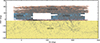 |
Fig. 1. Angular distribution of H I sources in FASHI sky (orange area), ALFALFA sky (blue area), and HIPASS (yellow area) sky. Grey points indicate individual detections. As the sky coverage of FASHI survey is not uniform, we split it into several pixels, each with an area of 2 deg2. In cases where there is an overlap between two surveys, we present the areas with deeper coverage. |
Details of samples we adopted in three surveys, including redshift ranges, sample sizes, Dec. ranges, and sky areas.
2.1. HIPASS
HIPASS was carried out with the Parkes 64 m radio telescope in Australia. It is the first blind H I survey to cover the entire southern sky with the declination ranging from −90° to +2° (Meyer et al. 2004). The HIPASS survey also has a northern extension catalogue covering the range of +2° < Dec < +25.5° (Wong et al. 2006), but it was not included in the HIMF calculation (Zwaan et al. 2005). It provides the largest uniform H I catalogue in the southern sky, with 4315 sources in the redshift range of −1280 km s−1 < cz ⊙ < 12 700 km s−1. The Parkes beam diameter is 15.5 arcmin at 21 cm, and the root-mean-square (rms) noise of HIPASS is 13.3 mJy beam−1 at a velocity resolution of 26.4 km s−1. As a first-generation survey, the mean depth of HIPASS was relatively shallow and it also suffers from a particularly large beam size (which can lead to source confusion and blending). In this paper, we limit the HIPASS sample to the declination range of −90° < Dec < 6.5° to avoid overlap with the FASHI south data.
2.2. ALFALFA
ALFALFA is a second-generation H I survey using the 305 m Arecibo single-dish telescope. Compared to HIPASS, it is evident that ALFALFA has a much smaller beam diameter (3.8 arcmin at 21 cm) and the rms noise level is significantly improved (2.4 mJy per beam at a velocity resolution of 10 km s−1). The final data release includes ∼31 500 extragalactic sources and covers almost 6900 deg2 of the northern sky in the redshift range of −2000 km s−1 < c z⊙ < 18 000 km s−1 (Haynes et al. 2018). The ALFALFA footprint is split into two continuous regions, which are named the ‘spring sky’ with right ascension (RA) ranges in 07h30m < RA < 16h 30m and ‘fall sky’ ranges in 22h < RA < 03h according to their observation seasons. The declination ranges from 0° to 36° in both regions. A drift scan strategy was employed to observe both regions, resulting in high time efficiency and uniform coverage. In this paper, we only include the Code 1 sources (signal-to-noise ratio larger than 6.5) in the ALFALFA catalogue, as the reliability is close to 100% (Saintonge 2007). We follow the boundary cuts as in Jones et al. (2018) and limit the declination range to less than 30° to avoid overlap with FASHI. To be consistent with the HIMF measurement of Jones et al. (2018), we also limit the redshift range of ALFALFA to 0 < z < 0.05, beyond which radio frequency interference (RFI) becomes more severe.
2.3. FASHI
Based on the FAST 500-m single-dish radio telescope, FASHI has achieved a greater survey depth compared to both HIPASS and ALFALFA, as well as the smaller beam size (effectively 3.24 arcmin at 21 cm; Wang et al. 2023, 2024) and much lower rms noise level (1.5 mJy per beam at 6.4 km s−1 resolution; Zhang et al. 2024). FASHI was designed to observe the entire detectable sky of FAST in the declination range of −14° < Dec < +66° (around 22 000 deg2). The first data release (Zhang et al. 2024) covers two separate regions, which we refer to as ‘FASHI north’ (30° < Dec < 66°) and ‘FASHI south’ (−6.2° < Dec < 0°), both with the right ascension in the ranges of 0h ≤ RA ≤ 17.3h and 22h ≤ RA ≤ 24h. The observed redshift range of FASHI is 200 km s−1 < c z⊙ < 26323 km s−1 with a frequency range of 1305.5–1419.5 MHz. However, this frequency range includes radio recombination lines, which are produced by gas ionised by young massive stars within H II regions of the Milky Way. To identify and eliminate these lines from the FASHI data, they used the criteria to ensure that the same spatial location exhibits consistent flux density and line width across various transition frequencies. In total, 41 741 extragalactic sources have been detected. For fair comparisons with ALFALFA, we adopt the same redshift limits as 0 < z < 0.05. Although FASHI observed quite a few galaxies in 0.05 < z < 0.09, the influence of RFI there would be much more significant for our HIMF measurements.
Unlike ALFALFA, FASHI is carried out in a time-filler mode, that is, the observations are made when there were no other running programmes in the observing queue. This observation strategy made full use of the available time to increase the sample size, but results in an inhomogeneous survey depth. The sky areas sampled multiple times would be much deeper than in other regions. As shown in Fig. 5 of Zhang et al. (2024), the detection rms noise (in units of mJy per beam) varied strongly in different parts of the sky, as well as between FASHI north and FASHI south. FASHI south has a significantly higher detection rms noise (i.e. much lower source surface densities). Therefore, in this study, we decided to treat FASHI north and FASHI south as two separate samples.
The problem of inhomogeneous sky coverage of FASHI is similar to that of angular variations of observed galaxy surface number densities due to the foreground stars in optical surveys. Therefore, we followed the strategy of Xu et al. (2023) by applying correction weights to galaxies in different areas. To do so, we split the FASHI sky coverage into grid pixels of equal area of 2 deg2, which roughly matches the typical scale of the rms noise variation. Since the FASHI drift scans were performed at a fixed sky declination, we constructed the pixels in linear declination bins of ΔDec. = 0.5° and adjusted the number of R.A. bins in different Dec. bins to reach the same pixel area. The resulting sky coverage of FASHI north and FASHI south is shown as the red regions in Fig. 1. The distribution at the edge of the survey is discrete, but will be much improved in the future FASHI data release.
Ideally, for a homogeneous H I survey, there should be no strong spatial variation in the surface number densities of galaxies. A correction factor of the galaxy surface density in each pixel is needed to derive the correct HIMF for FASHI. To find it, we first calculated the galaxy surface number density ( ) and the median rms noise for each pixel. In the left panel of Fig. 2, we show the normalised surface number density,
  , as a function of the median rms noise of each pixel (blue line with errors), where
  is the average surface number density of the entire sample. It is evident that without any correction, the detected number of galaxies in each pixel is highly correlated with the rms noise level. More galaxies tend to be found in regions that have been scanned multiple times (with lower rms noise). To correct for this effect, we adopt a second-order polynomial function to fit the rms noise dependence and weight galaxy by the reciprocal of the best-fitting function. We note that the assignment of the correction factor is pixel-wise (i.e. all galaxies in the same pixel share the same weight). Galaxies in the high (low) surface density regions are therefore down-weighted (up-weighted). After applying the correction factor (denoted as frms and applied in the following calculation of the HIMF in Eq. (5)), the weighted source surface density is almost homogeneous (red line). The weights in different pixels for FASHI north are shown in the right panel of Fig. 2. Most of the weights are in the range of 0.5–2 and we discarded all pixels with weights larger than 2 to refrain from heavily weighting galaxies in less-sampled regions. The weights for FASHI north and FASHI south were calculated independently, based on their own galaxy samples.
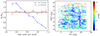 |
Fig. 2. Weights of FASHI north galaxies. Left panel: Blue line shows the normalised surface density as a function of the rms noise of the FASHI galaxies in each pixel. We weighted each galaxy with the reciprocal of the best-fitting rms noise dependence function to correct the surface density to be homogeneous, shown as red line. Right panel: Weights in different pixels for FASHI north. We only used pixels with the weights in the range of 0.5–2 to prevent heavily weighted galaxies ending up assigned to less-sampled regions. |
3. Methods
The H I mass of each galaxy is determined from the flux following the standard equation (Meyer et al. 2017):
 (2)
(2)
where S21 is the integrated H I flux in units of Jy km s−1 and DL(z) is the luminosity distance to the galaxy in units of Mpc. In order to minimise systematic uncertainties, we recalculated the H I mass in three catalogues in the same manner.
3.1. Distance estimates
One of the main systematics of determining MH I is the uncertainty of DL(z). Pure Hubble flow distances are commonly used for c z⊙ > 6000 km s−1 (Zwaan et al. 2005; Haynes et al. 2011), where the contribution of the peculiar velocity is relatively small. However, different flow models adopted to estimate peculiar velocities at c z⊙ < 6000 km s−1 could potentially cause large systematic uncertainties in DL(z) (Masters et al. 2004). Masters (2005) proposed a Local Volume flow model to reduce the distance errors by considering the infall of galaxies onto local superclusters. However, the distinct bias related to the line-of-sight galaxy density distribution, known as the Malmquist bias (Lynden-Bell et al. 1988), will lead to incorrect assignment of peculiar velocities (Strauss & Willick 1995).
The Cosmicflows-4 Distance–Velocity Calculator (Kourkchi et al. 2020)1 is designed to mitigate Malmquist bias and the asymmetry in velocity errors in translations to distance from the logarithmic modulus. It is based on the Cosmicflows-4 catalogue (Tully et al. 2023) and consists of two calculators. One is based on the smoothed velocity field from the numerical action methods (NAM; Shaya et al. 2017) model, but is limited only to a distance of 38 Mpc. The other CF4 calculator is based on the Wiener filter model (Valade et al. 2024) and extends to 500 Mpc.
The original HIPASS catalogue used the pure Hubble flow distances (Meyer et al. 2004; Zwaan et al. 2005) and ALFALFA adopted a local volume flow model of Masters (2005) for c z⊙ < 6000 km s−1. FASHI used the NAM model of Cosmicflows-3 Distance–Velocity Calculator for c z⊙ < 2400 km s−1 and the CF3 model (Graziani et al. 2019) for 2400 km s−1 < c z⊙ < 15 000 km s−1 and the pure Hubble flow for c z⊙ > 15 000 km s−1. In this work, we applied the updated Cosmicflows-4 model of Valade et al. (2024) to all three catalogues. As shown in Sect. 5.1, the influence of different flow models on the HIMF measurements in this study is minor.
3.2. Sample completeness
The completeness of the H I sample is the main uncertainty when estimating the HIMF. One way to estimate completeness is to insert a large number of synthetic sources into the data. The completeness can then be determined from the rate of recovered synthetic sources (Rosenberg & Schneider 2002; Zwaan et al. 2004). In this study, we followed the method of Haynes et al. (2011), using concrete data to calculate the completeness limits for three surveys. Since completeness is a function of both S21 and W50, we divided log W50 into 20 bins from 1.0 to 3.0 with a bin width of 0.1. In each log W50 bin, we calculated the surface number density of galaxies in logarithmic intervals of S21, dn/dlog S21, as a function of log S21. The surface density, rather than the number of galaxies in each log S21 bin as in Fig. 11 of Haynes et al. (2011), is used to make fair comparisons among samples from different survey areas.
We show the measurements of  in three representative log W50 bins in Fig. 3. As discussed in Haynes et al. (2011), the galaxy surface density, dn/dlog S21, would be proportional to
  for a complete sample. The deviation from a constant value of
  marks the start of incompleteness. Following Haynes et al. (2011), we can use an error function to fit the completeness C(S21|W50) in each W50 bin,
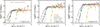 |
Fig. 3. Distribution of |

![Mathematical equation: $$ \begin{aligned} C(S_{21}|W_{50}) = \frac{1}{2}\left[1+\mathrm{erf} \left(\frac{\log S_{21}-\log S_{21,50\%}}{\sigma _{\log S_{21}}}\right)\right] ,\end{aligned} $$](/articles/aa/full_html/2025/03/aa52976-24/aa52976-24-eq17.gif) (3)
(3)
where the two free parameters are S21, 50% and σlog S21. Here, S21, 50% is the 50% completeness limit in a given W50 bin (i.e. C(S21|W50) = 0.5 when S21 = S21, 50%) and σlog S21 characterises the slope of decreasing completeness at the low-S21 end. In addition, we used a free parameter Ap to fit the plateau value of  in each W50 bin. The best-fitting curves are shown as solid lines in Fig. 3. The 50% completeness limit S21, 50% in each W50 bin of FASHI north is shown as the vertical dotted line.
It is remarkable that ALFALFA, FASHI north, and FASHI south share the same plateau value of  in each W50 bin, which demonstrates the reliability of the FASHI measurements. The HIPASS sample has consistently lower plateaus than other surveys because it is limited to a smaller volume (z < 0.042 rather than z < 0.05), which leads to lower surface densities. It is clear from the comparisons that FASHI north has the lowest rms noise, reaching a low flux density of S21 ∼ 0.1 Jy km s−1, which is about 0.5 dex deeper than ALFALFA. HIPASS is considerably shallower than other surveys and only detects high S21 sources. ALFALFA and FASHI south have comparable survey depths, which validates our separate treatments of FASHI north and FASHI south.
In Fig. 4, we show the dependence of S21, 50% on W50 as red circles for the four H I samples. The galaxy distribution in each sample is shown as the blue points. It is interesting to note that most galaxies in ALFALFA and HIPASS are above the 50% completeness limits. However, for FASHI north and FASHI south, there is still a large fraction of galaxies below the limits. This is related to the shallow slopes, σlog S21, seen in Fig. 3. In Table 2, we list the numbers of galaxies above and below the 50% completeness cuts in the four samples. The fraction of galaxies below the cuts are about 17%, 9%, 45%, and 34% for HIPASS, ALFALFA, FASHI north, and FASHI south, respectively. Although FASHI is able to detect galaxies with low S21, they are very incomplete. To avoid large corrections to low-completeness galaxies, we only used galaxies with C(S21|W50) > 0.5 to measure the HIMF. Currently, the fraction of discarded galaxies below the limits is quite large for FASHI, but it will be improved in the future with better sampling rates.
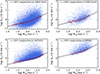 |
Fig. 4. Distribution of FASHI north (top-left), FASHI south (top-right), ALFALFA (bottom-left), and HIPASS (bottom-right) galaxies in the log S21–log W50 plane. The blue dots are all galaxy samples in each survey. The red open circles are the log S21 limit of 50% completeness in each log W50 bin. The black solid lines are the fitted broken power law relations. |
As in Haynes et al. (2011), we also find that the function of S21, 50%(W50) can be well fitted with a broken power law, as follows,
 (4)
(4)
where a1 and a2 are the free parameters. The transition W50 value, Wcut, is simply 2(a2 − a1). The best-fitting relations of the 50% completeness limits are shown as solid lines in Fig. 4 and the parameters are listed in Table 2. Our derived values of a1 and a2 for ALFALFA differ slightly from those of Haynes et al. (2011), namely: a1 = 1.207 and a2 = 2.457). This is because their measurements were based on the early sample of 40% ALFALFA. Our values align well with those reported in Oman (2022), a1 = 1.170 and a2 = 2.420), which are also based on the ALFALFA 100% sample.
3.3. Calculation method for HIMF
To derive the HIMF, it is also necessary to know the detectable volume for each galaxy. The HIMF is commonly measured with the two-dimensional stepwise maximum likelihood (2DSWML) method (e.g. Efstathiou et al. 1988; Zwaan et al. 2005; Martin et al. 2010; Jones et al. 2018) by calculating the effective volume, Veff, for each galaxy, which is often referred to as the 1/Veff method. The effective volume is obtained by maximising the joint likelihood of finding all sample galaxies in different MH I and W50 bins and also applied in a non-parametric way (i.e. without assuming a functional form of the HIMF) and in correlation to the galaxy space density. As extensively discussed in Martin et al. (2010), the 1/Veff method has the advantage of being robust against density fluctuations in the large-scale structure, compared to the traditional 1/Vmax method (Schmidt 1968). However, the 1/Veff method is very sensitive to the exact completeness cut. As shown in Fig. 1 of Oman (2022), the HIMF of ALFALFA measured with the 1/Veff method is much higher at the low-mass end because it uses a 0.02 dex higher S21, 50% cut from the ALFALFA 100% sample, compared to the old cut from the 40% sample.
On the other hand, the main bias in the 1/Vmax method is the influence of large-scale structures. The ALFALFA volume covers the Virgo Cluster and the Local Supercluster, where the number densities of galaxies with low MH I are much higher than those of other regions. The estimated HIMF using 1/Vmax would be systematically overestimated at the low-mass end without corrections (Martin et al. 2010), which motivates the use of the 1/Veff method to measure the HIMF for ALFALFA. The application of the 1/Veff method is based on the density variation within a given survey volume. Therefore, it still suffers from the effect of large-scale structures when applied to H I samples in different survey volumes. For example, for the ALFALFA survey, there are large differences between the HIMFs of the spring and fall sky regions derived separately using the 1/Veff method (see Fig. 3 of Jones et al. 2018). A homogeneous H I sample that covers a very large survey volume is ideal for applying the 1/Veff method to derive the intrinsic HIMF.
In this paper, by combining three surveys that cover almost 76% of the entire sky in the Local Universe, the influence of large-scale structures is effectively suppressed for both the 1/Veff and 1/Vmax methods. However, the 1/Veff method is not directly applicable in this case because the three surveys have completely different selection functions, as shown in Fig. 4. When using the 1/Veff method for the combined sample, it would be diffcult to make a fair comparison of the likelihood of finding galaxies in different survey volumes. Therefore, we chose to apply the 1/Vmax method to measure the total HIMF.
The Vmax value of each galaxy is simply obtained from the maximum distance that the galaxy can be observed with the 50% completeness limit. Since the HIPASS sample is limited to a slightly smaller redshift of z < 0.042, we can assume that there is no evolution within the redshift range of 0.042 < z < 0.05. The final HIMF can be obtained as,
 (5)
(5)
where C(S21, i|W50, i) is the completeness of the i-th galaxy with a flux density, S21, i, and a line profile width W50, i. Then, Vmax, i is the corresponding maximum volume and frms, i is the rms noise correction factor for each galaxy in FASHI calculated in Fig. 2, which we set to 1 for ALFALFA and HIPASS. The sum is over all galaxies in a given MH I bin. When combining the four samples, we calculated Vmax for each galaxy using the total sky area of 31 528 deg2. We note that we only selected galaxies above the 50% completeness cut and the incompleteness effect is taken into account in Eq. 5 with the weight of 1/C(S21, i) for each galaxy.
4. H I mass function
In the left panel of Fig. 5, we show the total HIMF as open circles, along with our measurements of the HIMFs calculated using the same methods for the individual surveys of ALFALFA, HIPASS, FASHI north, and FASHI south using solid lines of different colours. All measurements are listed in Table 3. The cosmic variance effect is weak for MH I > 1010 M⊙, where the individual HIMFs of different samples are consistent with each other. These galaxies are probed to larger volumes, and thus less affected by the large-scale structures. However, the discrepancies become much larger at the lower-mass end, especially for MH I < 108 M⊙. In fact, even for the deepest FASHI north sample, galaxies with MH I < 108 M⊙ are only detected within 50 Mpc, which leads to the large variation of HIMFs at the low-mass end.
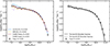 |
Fig. 5. Left: H I mass functions of ALFALFA, HIPASS, and FASHI north and FASHI south, shown as blue, orange, red, and purple solid lines, respectively. The total HIMF by combining three surveys is shown as black open circles with error bars. Right: Best-fit Schechter function (black solid line) and 2D Schechter function (black dashed lines). |
HIMFs of the three surveys and the total results of their combination.
It is interesting that the HIMFs of ALFALFA and FASHI north are consistently higher than those of HIPASS and FASHI south for MH I < 1010 M⊙. This reflects the differences in the large-scale structures of the northern and southern skies. As mentioned above, the superclusters in the northern sky will lead to the overestimate of the HIMF at the low-mass end, whereas the voids presented in the southern sky will cause the underestimate, such as the Local Void (around RA ∼ 270° and Dec. ∼ −30°) in the HIPASS footprint (Meyer et al. 2004). Combining the measurements in different surveys of various large-scale structures has significantly improved the estimates of the HIMF in the Local Universe.
For the total HIMF, the measurement errors would be less dominated by the cosmic variance effect, and more so by the Poisson noise caused by the limited numbers of galaxies. Therefore, we can approximate the variance for the total HIMF as in Jones et al. (2018), namely,
 (6)
(6)
Following common practice, we also fit a Schechter function to the total HIMF, shown as the solid line in the right panel of Fig. 5. The best-fitting parameters are α = −1.30 ± 0.01 and  and ϕs = (6.58 ± 0.23)×10−3 h703 Mpc−3dex−1. The best-fitting parameters for the total HIMF and each of the three surveys are presented in Table 4. However, this single Schechter fitting slightly underestimates the high-mass end of the HIMF (the largest H I mass bin). It has previously been suggested that a double Schechter function provides a much better fit to the galaxy stellar mass function at low redshifts, especially at the low-mass end (see e.g. Baldry et al. 2008; Tomczak et al. 2014). We also adopt the following double-Schechter function to fit the total HIMF,
HIMF fitting parameters for the three surveys and the total results of their combination.
 (7)
(7)
where the parameters (ϕs1, Ms1, α) and (ϕs2, Ms2, α) refer to the two Schechter components with the same slope α, respectively. Shown as a dashed line in the right panel of Fig. 5, it provides a better fit than a single Schechter function, especially at the high-mass end. We find that the total HIMF is better fitted with the same slope, α, and two different ‘knee’ masses, Ms1 and Ms2. The best-fitting reduced χ2 (i.e. χ2/d.o.f.) decreases from 56/17 for the single-Schechter function to 24/15 for the double-Schechter function. The best-fitting parameters are ϕs1 = (2.67 ± 0.98)×10−3 h703 Mpc−3 dex−1,  , ϕs2 = (5.96 ± 0.78)×10−3 h703 Mpc−3 dex−1,
  , and α = −1.24 ± 0.02. The two different ‘knee’ masses are likely associated with different galaxy populations, for example, central and satellite galaxies. It will be further confirmed in our future work with the decomposition of HIMF into central and satellite galaxies.
The cosmic H I abundance, ΩH I, can be estimated by integrating the best-fitting single Schechter function as follows (Martin et al. 2010; Jones et al. 2018),
 (8)
(8)
where ρc is the critical density at z = 0 (we assume H0 = 70h70 km s−1 Mpc−1). This gives  , which is almost the same for double Schechter function fits.
5. Discussion
5.1. Distance uncertainties
As discussed in previous sections, measurement errors in distance estimates could potentially lead to systematic uncertainties in the HIMF (Masters et al. 2004). To investigate the effects of distance estimates, we followed the practice of Jones et al. (2018) to measure the HIMFs by applying different flow models. In Fig. 6, we compare the total HIMFs calculated using different distance models, including the pure Hubble flow (blue line: assuming H0 = 70h70 km s−1 Mpc−1), the flow model of Masters (2005), orange line): the NAM model (red line), and the CF4 model (adopted in this work) in the Cosmicflows-4 Distance–Velocity Calculator. The distance estimates in the NAM model are limited to 38 Mpc, whereas the CF4 model extends this limit to 500 Mpc. The flow model of Masters (2005) is also limited to a distance of c z⊙ < 6000 km s−1 as in the ALFALFA sample. For galaxies lying beyond these distances, we utilised the pure Hubble flow.
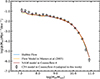 |
Fig. 6. Total H I mass functions calculated by different distance estimate models. The pure Hubble Flow, flow model in Masters (2005), NAM model and CF4 model in Cosmicflow-4 (adopted in our work) are shown as blue, orange, red solid lines, and black open circles with their errorbars, respectively. |
The HIMF with the CF4 model is consistent with all other models for MH I > 109 M⊙, but is slightly higher at the low-mass end. As shown in Tully et al. (2023), by including the kinematic information of ALFALFA, the peculiar velocities in Cosmicflows-4 are much improved compared to Cosmicflows-3. The maximum difference in these distance estimates for MH I < 108 M⊙ is around Δlog DL ∼ 0.08, which will introduce an offset of 0.16 dex in the H I mass at the low-mass end. Since the HIMF at the low-mass end is  , the 0.16 dex offset in MH I will translate to a minor offset of 0.048 dex in ϕ(MH I) for α = −1.30. The small number of galaxies at the low-mass end also limits our ability to tightly constrain the HIMF here. For the massive end, the effects of different flow models are weaker with respect to the pure Hubble flow. Therefore, we can conclude that the effect of different distance estimates would not substantially change the measured HIMF, consistent with the results shown in Jones et al. (2018).
5.2. Comparison with the literature
In Fig. 7, we compare our HIMF measurement (open circles) with those of HIPASS from Zwaan et al. (2005), ALFALFA from Guo et al. (2023), Arecibo Ultra-Deep Survey (AUDS) from Xi et al. (2021), and MIGHTEE-HI from Ponomareva et al. (2023).
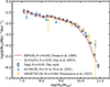 |
Fig. 7. Comparisons of HIMF in a range of literature works. Measurements of HIPASS in Zwaan et al. (2005), ALFALFA in Guo et al. (2023), AUDS100 in Xi et al. (2021), and MIGHTEE–HI in Ponomareva et al. (2023) are shown as the red solid line, purple solid line, blue triangles, and yellow diamonds, respectively. The total HIMF derived in this work are shown as black open circles with error bars. |
The HIMF of HIPASS in Zwaan et al. (2005) shows a slightly lower high-mass end amplitude. We note that their original HIMF measurements used a higher Hubble constant of H0 = 75h75 km s−1 Mpc−1. For consistency with our definition of H0 = 70h70 km s−1 Mpc−1, we applied approximate corrections to increase their MH I by 0.06 dex and decreasing ϕ(MH I) by −0.09 dex. The underestimation of ϕ(MH I) at the high-mass end could then be caused by uncertainties in the completeness function and the HIMF normalisation estimation method (Zwaan et al. 2003). They adopted a different completeness estimation method using the recovered rates of the inserted synthetic sources (Zwaan et al. 2004). In their 2DSWML method, the overall normalisation of HIMF is lost in the maximum likelihood estimator and is then determined from the mean galaxy number density with the minimum variance estimator (Zwaan et al. 2005).
The HIMF measurement of Guo et al. (2023) used the ALFALFA 100% sample and corrected for the incompleteness effect in Jones et al. (2018) by using the 90% completeness cut S21, 90% of Haynes et al. (2011). Their HIMF and  results are quite consistent with ours. We also show the AUDS measurement of Xi et al. (2021) that extends to a slightly higher redshift of z = 0.16. It shows a mild redshift evolution of the HIMF, with a shallower slope at the high-mass end. However, their H I detection only included 247 galaxies in a sky area of 1.35deg2. The small number of galaxies limits an accurate determination of the HIMF. However, they found
  , which is consistent with our ΩH I measurement. Ponomareva et al. (2023) measured the HIMF using the MIGHTEE-HI survey in a redshift range of 0 ≤ z ≤ 0.084. They also found slightly higher ϕ(MH I) amplitudes in MH I > 1010 M⊙ than in the z = 0 measurements. Their ΩH I measurement is slightly larger, with
  , albeit with large errors. These measurements tend to point to the weak evolution of ΩH I in 0 < z < 0.2 (Rhee et al. 2018; Walter et al. 2020), consistent with the prediction of the theoretical model (Guo et al. 2023). Ongoing and future deep H I observations, for example, the FAST Ultra-Deep Survey (Xi et al. 2024), will provide more insight into the evolution of the HIMF.
We note that the HIMF of our total sample is consistent with the HIMF of Guo et al. (2023). However, from the best-fitting Schechter function fits displayed in Table 4, the relevant fitting parameters are slightly different. We have a slightly lower ‘knee’ mass of  , while it is reported as
  in Guo et al. (2023). However, as shown in Fig. 4 of Ponomareva et al. (2023), the three parameters of the Schechter function are strongly correlated with each other, with Ms showing anticorrelations with α and ϕs. Comparisons between the parameters of Schechter function fits of different samples should not be treated independently.
6. Conclusions
In this study, we measured the H I mass function in the Local Universe (0 < z < 0.05) by combining the H I samples in the HIPASS, ALFALFA and FASHI surveys, covering 76% of the entire sky (31 528 deg2). The combined sample has the advantage of greatly suppressing the influence of cosmic variance on the measured HIMF. To further reduce systematic uncertainties in the processing of the H I catalogues, we adopted the same methods to estimate distances, calculate sample completeness, and determine the HIMF (the 1/Vmax method) for all three catalogues. We measured the most complete HIMF in the Local Universe so far (Fig. 5) and obtained the first HIMF measurement for the recent FASHI survey, presented here.
We fit the total HIMF with a single Schechter function, with the parameters of α = −1.30 ± 0.01 and  and ϕs = (6.58 ± 0.23)×10−3 h703 Mpc−3 dex−1. The derived cosmic H I abundance is
  , which is consistent with the measurement using the ALFALFA 100% complete sample (Guo et al. 2023). However, we find that our HIMF is better described by a double Schechter function with the same slope α. The best-fitting parameters are ϕs1 = (2.67 ± 0.98)×10−3 h703 Mpc−3 dex−1,
  , ϕs2 = (5.96 ± 0.78)×10−3 h703 Mpc−3 dex−1,
  , and α = −1.24 ± 0.02. The two different ‘knee’ masses are favoured by the measured HIMF at the massive end, indicating contributions from two different components (likely from the central and satellite galaxies).
We found that the measured HIMF is marginally affected by the choice of distance estimates. We adopted different flow models to estimate the luminosity distances and obtained fully consistent results. However, local large-scale structures have a strong influence on the HIMF when measured separately in different H I samples, especially at the low-mass end. ALFALFA and FASHI north have consistently higher HIMFs than those of HIPASS and FASHI south, due to the influence of local superclusters. Combining the three H I surveys provides a unique opportunity to obtain an unbiased estimate of the HIMF in the Local Universe.
We note that although the combined sample covers a large sky area, galaxies with low MH I have been probed within very limited volumes and with limited statistics. Deeper H I surveys in the near future will provide more robust measurements of HIMF at the low-mass end.
Acknowledgments
We thank the anonymous reviewer for the helpful comments that improved the presentation of this paper. This work is supported by the National SKA Program of China (grant No. 2020SKA0110100), the Guizhou Provincial Science and Technology Projects (QKHFQ[2023]003, QKHPTRC-ZDSYS[2023]003, QKHFQ[2024]001-1, QKHJC-ZK[2025]MS015) and the CAS Project for Young Scientists in Basic Research (No. YSBR-092). We acknowledge the use of the High Performance Computing Resource in the Core Facility for Advanced Research Computing at the Shanghai Astronomical Observatory.
References
- Baldry, I. K., Glazebrook, K., & Driver, S. P. 2008, MNRAS, 388, 945 [NASA ADS] [Google Scholar]
- Barnes, D. G., Staveley-Smith, L., de Blok, W. J. G., et al. 2001, MNRAS, 322, 486 [Google Scholar]
- Baugh, C. M., Gonzalez-Perez, V., Lagos, C. d. P., et al. 2019, MNRAS, 483, 4922 [NASA ADS] [CrossRef] [Google Scholar]
- Davé, R., Crain, R. A., Stevens, A. R. H., et al. 2020, MNRAS, 497, 146 [Google Scholar]
- Efstathiou, G., Ellis, R. S., & Peterson, B. A. 1988, MNRAS, 232, 431 [Google Scholar]
- Fu, J., Kauffmann, G., Huang, M.-L., et al. 2013, MNRAS, 434, 1531 [NASA ADS] [CrossRef] [Google Scholar]
- Giovanelli, R., Haynes, M. P., Kent, B. R., et al. 2005, AJ, 130, 2598 [Google Scholar]
- Graziani, R., Courtois, H. M., Lavaux, G., et al. 2019, MNRAS, 488, 5438 [NASA ADS] [CrossRef] [Google Scholar]
- Guo, H., Jones, M. G., & Wang, J. 2022, ApJ, 933, L12 [NASA ADS] [CrossRef] [Google Scholar]
- Guo, H., Wang, J., Jones, M. G., & Behroozi, P. 2023, ApJ, 955, 57 [NASA ADS] [CrossRef] [Google Scholar]
- Haynes, M. P., Giovanelli, R., Martin, A. M., et al. 2011, AJ, 142, 170 [Google Scholar]
- Haynes, M. P., Giovanelli, R., Kent, B. R., et al. 2018, ApJ, 861, 49 [Google Scholar]
- Jarvis, M., Taylor, R., Agudo, I., et al. 2016, MeerKAT Science: On the Pathway to the SKA, 6 [Google Scholar]
- Jones, M. G., Haynes, M. P., Giovanelli, R., & Moorman, C. 2018, MNRAS, 477, 2 [Google Scholar]
- Jones, M. G., Hess, K. M., Adams, E. A. K., & Verdes-Montenegro, L. 2020, MNRAS, 494, 2090 [NASA ADS] [CrossRef] [Google Scholar]
- Kamphuis, P., Jütte, E., Heald, G. H., et al. 2022, A&A, 668, A182 [NASA ADS] [CrossRef] [EDP Sciences] [Google Scholar]
- Koribalski, B. S., Staveley-Smith, L., Westmeier, T., et al. 2020, Ap&SS, 365, 118 [Google Scholar]
- Kourkchi, E., Courtois, H. M., Graziani, R., et al. 2020, AJ, 159, 67 [NASA ADS] [CrossRef] [Google Scholar]
- Lynden-Bell, D., Faber, S. M., Burstein, D., et al. 1988, ApJ, 326, 19 [NASA ADS] [CrossRef] [Google Scholar]
- Ma, W., Guo, H., & Jones, M. G. 2024, A&A, 695, A5 [Google Scholar]
- Martin, A. M., Papastergis, E., Giovanelli, R., et al. 2010, ApJ, 723, 1359 [NASA ADS] [CrossRef] [Google Scholar]
- Masters, K. L. 2005, Ph.D. Thesis, Cornell University, New York, USA [Google Scholar]
- Masters, K. L., Haynes, M. P., & Giovanelli, R. 2004, ApJ, 607, L115 [NASA ADS] [Google Scholar]
- Meyer, M. J., Zwaan, M. A., Webster, R. L., et al. 2004, MNRAS, 350, 1195 [Google Scholar]
- Meyer, M., Robotham, A., Obreschkow, D., et al. 2017, PASA, 34, 52 [Google Scholar]
- Oman, K. A. 2022, MNRAS, 509, 3268 [Google Scholar]
- Péroux, C., & Howk, J. C. 2020, ARA&A, 58, 363 [CrossRef] [Google Scholar]
- Ponomareva, A. A., Jarvis, M. J., Pan, H., et al. 2023, MNRAS, 522, 5308 [NASA ADS] [Google Scholar]
- Popping, G., Caputi, K. I., Trager, S. C., et al. 2015, MNRAS, 454, 2258 [NASA ADS] [CrossRef] [Google Scholar]
- Rafieferantsoa, M., Davé, R., & Naab, T. 2019, MNRAS, 486, 5184 [NASA ADS] [CrossRef] [Google Scholar]
- Rhee, J., Lah, P., Briggs, F. H., et al. 2018, MNRAS, 473, 1879 [NASA ADS] [CrossRef] [Google Scholar]
- Rosenberg, J. L., & Schneider, S. E. 2002, ApJ, 567, 247 [NASA ADS] [CrossRef] [Google Scholar]
- Saintonge, A. 2007, AJ, 133, 2087 [NASA ADS] [CrossRef] [Google Scholar]
- Saintonge, A., & Catinella, B. 2022, ARA&A, 60, 319 [NASA ADS] [CrossRef] [Google Scholar]
- Schechter, P. 1976, ApJ, 203, 297 [Google Scholar]
- Schmidt, M. 1968, ApJ, 151, 393 [Google Scholar]
- Shaya, E. J., Tully, R. B., Hoffman, Y., & Pomarède, D. 2017, ApJ, 850, 207 [NASA ADS] [CrossRef] [Google Scholar]
- Strauss, M. A., & Willick, J. A. 1995, Phys. Rep., 261, 271 [NASA ADS] [CrossRef] [Google Scholar]
- Tomczak, A. R., Quadri, R. F., Tran, K.-V. H., et al. 2014, ApJ, 783, 85 [Google Scholar]
- Tully, R. B., Kourkchi, E., Courtois, H. M., et al. 2023, ApJ, 944, 94 [NASA ADS] [CrossRef] [Google Scholar]
- Valade, A., Libeskind, N. I., Pomarède, D., et al. 2024, Nat. Astron., 8, 1610 [Google Scholar]
- Walter, F., Carilli, C., Neeleman, M., et al. 2020, ApJ, 902, 111 [Google Scholar]
- Wang, L., Zheng, Z., Hao, C.-N., et al. 2022, MNRAS, 516, 2337 [NASA ADS] [CrossRef] [Google Scholar]
- Wang, J., Yang, D., Oh, S. H., et al. 2023, ApJ, 944, 102 [NASA ADS] [CrossRef] [Google Scholar]
- Wang, J., Lin, X., Yang, D., et al. 2024, ApJ, 968, 48 [NASA ADS] [CrossRef] [Google Scholar]
- Wong, O. I., Ryan-Weber, E. V., Garcia-Appadoo, D. A., et al. 2006, MNRAS, 371, 1855 [Google Scholar]
- Xi, H., Staveley-Smith, L., For, B.-Q., et al. 2021, MNRAS, 501, 4550 [NASA ADS] [Google Scholar]
- Xi, H., Peng, B., Staveley-Smith, L., et al. 2024, ApJS, 274, 18 [NASA ADS] [Google Scholar]
- Xie, L., De Lucia, G., Hirschmann, M., Fontanot, F., & Zoldan, A. 2017, MNRAS, 469, 968 [Google Scholar]
- Xu, H., Zhang, P., Peng, H., et al. 2023, MNRAS, 520, 161 [Google Scholar]
- Zhang, C.-P., Zhu, M., Jiang, P., et al. 2024, Sci. China Phys. Mech. Astron., 67, 219511 [NASA ADS] [CrossRef] [Google Scholar]
- Zwaan, M. A., Staveley-Smith, L., Koribalski, B. S., et al. 2003, AJ, 125, 2842 [Google Scholar]
- Zwaan, M. A., Meyer, M. J., Webster, R. L., et al. 2004, MNRAS, 350, 1210 [NASA ADS] [CrossRef] [Google Scholar]
- Zwaan, M. A., Meyer, M. J., Staveley-Smith, L., & Webster, R. L. 2005, MNRAS, 359, L30 [NASA ADS] [CrossRef] [Google Scholar]
All Tables
Details of samples we adopted in three surveys, including redshift ranges, sample sizes, Dec. ranges, and sky areas.
HIMF fitting parameters for the three surveys and the total results of their combination.
All Figures
|
Fig. 1. Angular distribution of H I sources in FASHI sky (orange area), ALFALFA sky (blue area), and HIPASS (yellow area) sky. Grey points indicate individual detections. As the sky coverage of FASHI survey is not uniform, we split it into several pixels, each with an area of 2 deg2. In cases where there is an overlap between two surveys, we present the areas with deeper coverage. |
| In the text | |
|
Fig. 2. Weights of FASHI north galaxies. Left panel: Blue line shows the normalised surface density as a function of the rms noise of the FASHI galaxies in each pixel. We weighted each galaxy with the reciprocal of the best-fitting rms noise dependence function to correct the surface density to be homogeneous, shown as red line. Right panel: Weights in different pixels for FASHI north. We only used pixels with the weights in the range of 0.5–2 to prevent heavily weighted galaxies ending up assigned to less-sampled regions. |
| In the text | |
|
Fig. 3. Distribution of |
| In the text | |
|
Fig. 4. Distribution of FASHI north (top-left), FASHI south (top-right), ALFALFA (bottom-left), and HIPASS (bottom-right) galaxies in the log S21–log W50 plane. The blue dots are all galaxy samples in each survey. The red open circles are the log S21 limit of 50% completeness in each log W50 bin. The black solid lines are the fitted broken power law relations. |
| In the text | |
|
Fig. 5. Left: H I mass functions of ALFALFA, HIPASS, and FASHI north and FASHI south, shown as blue, orange, red, and purple solid lines, respectively. The total HIMF by combining three surveys is shown as black open circles with error bars. Right: Best-fit Schechter function (black solid line) and 2D Schechter function (black dashed lines). |
| In the text | |
|
Fig. 6. Total H I mass functions calculated by different distance estimate models. The pure Hubble Flow, flow model in Masters (2005), NAM model and CF4 model in Cosmicflow-4 (adopted in our work) are shown as blue, orange, red solid lines, and black open circles with their errorbars, respectively. |
| In the text | |
|
Fig. 7. Comparisons of HIMF in a range of literature works. Measurements of HIPASS in Zwaan et al. (2005), ALFALFA in Guo et al. (2023), AUDS100 in Xi et al. (2021), and MIGHTEE–HI in Ponomareva et al. (2023) are shown as the red solid line, purple solid line, blue triangles, and yellow diamonds, respectively. The total HIMF derived in this work are shown as black open circles with error bars. |
| In the text | |
Current usage metrics show cumulative count of Article Views (full-text article views including HTML views, PDF and ePub downloads, according to the available data) and Abstracts Views on Vision4Press platform.
Data correspond to usage on the plateform after 2015. The current usage metrics is available 48-96 hours after online publication and is updated daily on week days.
Initial download of the metrics may take a while.