© ESO 2021

1. Introduction

In recent decades, diffuse X-ray emission associated with radio sources and extending beyond their host galaxies up to hundreds of kiloparsec scale, has recently been revealed by Chandra telescope at cosmological distances, that is, up to redshift 3.8 (4C 41.17; Scharf et al. 2003). A few recent examples are 3C 294 (Fabian et al. 2003), 3C 191 (Erlund et al. 2006), and 3CR 459 (Maselli et al. 2018). This diffuse X-ray emission is generally interpreted as due to inverse Compton (IC) scattering of nonthermal radio-emitting electrons on cosmic microwave background (CMB) photons, permeating their radio lobes (IC/CMB; Harris & Grindlay 1979; Schwartz et al. 2000; Tavecchio et al. 2000). This scenario is supported by the observational evidence that even without a clear morphological match between the radio and X-ray emission, extended X-ray structures are generally aligned to the radio axis and/or spatially coincident with radio structures. The lack of a clear radio counterpart to X-ray structures in high-redshift sources (Ghisellini et al. 2015) could be due to the increasing energy density of the CMB with z (Ghisellini et al. 2014), as U_CMB = 4.22 × 10⁻¹³ (1 + z)⁴) erg cm⁻³, corresponding to an equipartition magnetic field¹B_cmb = 3.25 (1 + z)² μG (Murgia et al. 1999; Massaro & Ajello 2011). If the average magnetic field in the lobe is less than B_cmb, the relativistic electrons in the lobe preferentially cool through IC/CMB rather than synchrotron radiation. This results in a dimming of radio emission while boosting the X-ray emission, which is a process known as CMB quenching (see, e.g., Celotti & Fabian 2004; Wu et al. 2017).

However, IC/CMB is not the only possible interpretation for this extended X-ray emission, since high-redshift radio galaxies are often used as tracers of galaxy clusters inhabiting galaxy poor or moderately rich environments (see, e.g., Worrall 2002, 2009; Crawford & Fabian 2003). Thus extended X-ray emission from these sources can be due to, or at least partially contaminated, by the thermal emission arising from the hot gas of the intergalactic medium (IGM; see, e.g., Ineson et al. 2013, 2015).

Disentangling scenarios of nonthermal emission via IC/CMB and thermal emission from hot gas in the IGM is however challenging. To shed a light on the nature of such diffuse X-ray emission two main tests can be performed.

The first would be to carry out radio observations at megahertz frequencies, where it would be possible to observe the synchrotron radiation of the same particles in the radio lobes responsible for the IC/CMB X-ray emission and thus verify if the spectral shape of the two components is consistent. Assuming that the X-ray radiation at 1 keV is due to IC/CMB and that the emission in radio lobes is unbeamed, the synchrotron radiation from the same electrons would be observed at radio frequencies

$$\begin{array}{c}\hfill {\nu }_{\mathrm{syn}}=1.44(B/\mathrm{\mu }\mathrm{G}){(1+z)}^{-1}\mathrm{MHz},\end{array}$$(1)

where z is the source redshift and B is the average magnetic field in the lobe (e.g., Felten & Morrison 1966), or equivalently ν_syn = 4.68 b (1 + z) MHz, where b is the ratio of B and B_cmb. For magnetic fields of the order of tens of microgauss (e.g., Scharf et al. 2003; Erlund et al. 2006), ν_syn would fall at MHz frequencies. In this case, we would expect the photon index measured in X-ray, Γ, to be related to the spectral index measured at MHz frequencies α by the relation Γ = 1 − α (e.g., Smail et al. 2012). This test, however, cannot be directly carried out because current and future low radio frequency facilities such as the Low-Frequency Array (LOFAR; van Haarlem et al. 2013), the Murchison Widefield Array (MWA; Bowman et al. 2013), the Long Wavelength Array (LWA; Ellingson et al. 2009), the Giant Metrewave Radio Telescope (GMRT; Swarup 1991), the Karl G. Jansky Very Large Array (JVLA; Perley et al. 2011) and the Square Kilometre Array (SKA; Dewdney et al. 2009) could only skim the desired radio frequency range. For example, observing the synchrotron radiation from the same electrons responsible for the IC/CMB emission in X-rays in a 50 MHz LOFAR observation of a z ∼ 2 source would require a magnetic field in the radio lobes B > 100 μG that is larger than those estimated as ∼25 μG by Erlund et al. (2006). For 4C 41.17 (z = 3.8), we would need B > 170 μG, which is still larger than the maximum equipartition magnetic field estimated for this source (Carilli et al. 1998; Scharf et al. 2003).

The second scenario is a X-ray spectral analysis to check if the spectrum at energies of a few kilo-electronvolts shows a thermal continuum and possibly emission lines or if instead the spectrum appears to have a nonthermal origin, such as in the form of a steep power law with photon index ∼2, as observed in lobes of radio galaxies (see, e.g., Croston et al. 2005; Hardcastle et al. 2006; Mingo et al. 2017). We note however that this test in general does not allow us to discriminate between the different models only by comparing fit statistics, even in cases of sources with large number of counts (Hardcastle & Croston 2010).

In the last decade, we carried out the Chandra snapshot survey of the Third Cambridge catalog (3C; Bennett 1962) to guarantee the complete X-ray coverage of the entire 3CR catalog (Massaro et al. 2010, 2012, 2015). We discovered X-ray emission associated with radio jets (see, e.g., Massaro et al. 2009a), hotspots (see, e.g., Massaro et al. 2011; Orienti et al. 2012), and diffuse X-ray emission from hot atmospheres and IGM in galaxy clusters (see, e.g., Hardcastle et al. 2010, 2012; Dasadia et al. 2016; Ricci et al. 2018), extended X-ray emission aligned with the radio axis of several moderate and high-redshift radio galaxies (see, e.g., Massaro et al. 2013, 2018; Stuardi et al. 2018; Jimenez-Gallardo et al. 2020), and the presence of extended X-ray emission spatially associated with optical emission line regions not coincident with radio structures, as in 3CR 171 and 3CR 305 (Massaro et al. 2009b; Hardcastle et al. 2010, 2012; Balmaverde et al. 2012). One of the best examples of the latter discovery is 3C 187. This Fanaroff-Riley (FR; Fanaroff & Riley 1974) II radio galaxy is, among those pointed in our snapshot survey, the brightest one showing extended X-ray emission on hundreds of kpc. Massaro et al. (2013) claimed that such diffuse X-ray emission in 3C 187 is consistent with the lobe radio structure. In this work, on the basis of additional information collected from the literature, we present a thorough investigation of its X-ray emission and a comparison with the optical information.

Extending the analysis by Massaro et al. (2013), we present surface flux profiles of the X-ray emission to evaluate its extension and estimate its properties. We perform X-ray spectral analysis coupled with a comparison with IC/CMB model to test the nonthermal scenario. Moreover, we investigate the presence of a galaxy cluster claimed in the literature via a procedure based on the red sequence (Visvanathan & Sandage 1977; Gladders et al. 1998). To this end, we performed optical spectroscopic observation of sources in the field of 3C 187 with the Victor Blanco Telescope in Cerro Tololo, Chile. However, as a consequence of bad observing conditions we were only able to collect spectra for 23 bright sources.

The paper is organized as follows. A brief multifrequency description of 3C 187 is given in Sect. 2. The Chandra data reduction and analysis are presented in Sect. 3. Results on possible X-ray emission mechanisms and the presence of a galaxy cluster are discussed in Sect. 4, while Sect. 5 is devoted to our conclusions. Unless otherwise stated we adopt cgs units for numerical results and we also assume a flat cosmology with H₀ = 69.6 km s⁻¹ Mpc⁻¹, Ω_M = 0.286, and Ω_Λ = 0.714 (Bennett et al. 2014). Spectral indexes, α, are defined by flux density, F_ν ∝ ν^−α both in radio and in the X-rays. Pan-STARRS magnitudes are in the AB system (Tonry et al. 2012).

2. Source description

3C 187 is a radio galaxy with a flux density at 178 MHz of 8.1 Jy (Smith & Spinrad 1980) and therefore sits at the lower end of FR II observed radio powers (e.g., Black et al. 1992). In the 3C catalog (Smith & Spinrad 1980), 3C 187 was identified as an optical source at z = 0.350 based on the 4000 Å break and G band absorption. Hutchings et al. (1988), using the Canada France Hawaii Telescope (CFHT) data, measured a magnitude m_R = 20.7 for this optical source and reported that the source appears to be elliptical without any obvious structure. These authors also found that the source appears to be a member of a cluster of ∼30 similarly extended objects projected between the radio lobes, as also stated by Neff et al. (1995).

Imaging with VLA (Bogers et al. 1994) revealed a triple radio source for 3C 187, with a faint core and two lobes separated by $\sim 2\stackrel{\prime }{.}0$ along a position angle P.A. = −21°². In particular, Rhee et al. (1996) reported 1.4 GHz flux densities of 246 and 312 mJy for the north and south lobes, respectively. Neff et al. (1995) reported 1.4 GHz flux densities of 4, 463, and 459 mJy for the core, north lobe, and south lobe, respectively, and 5 GHz flux densities of 3, 44, and 26 mJy for the core, north lobe, and south lobe, respectively.

The optical identification of Smith & Spinrad (1980) was therefore revised by Hes et al. (1995), who proposed the identification of 3C 187 core with an optical source coincident with the radio core observed in the radio maps presented by Bogers et al. (1994), which has m_R = 20.0 and a redshift of z = 0.465, based on [OII] and [OIII] emission lines, as well as a 4000 Å break. In the following we adopt this redshift for 3C 187³.

A Chandra snapshot observation of ∼12 ks was performed in January 2012 and analyzed in Massaro et al. (2013). These authors report extended X-ray emission that is co-spatial with the radio structure, detected with high significance (> 7σ) in four regions coincident with and between the radio lobes (see their Fig. 2). In the following we reanalyze these Chandra data and their correlation with the radio emission.

3. X-ray data reduction and analysis

The Chandra observation of 3C 187 was retrieved from the Chandra Data Archive through the ChaSeR service⁴. This consists of a single 12 ks observation (OBSID 13875; PI: Massaro, GO 13) carried out on January 2012 in VFAINT mode. These data were analyzed with the CIAO (Fruscione et al. 2006) data analysis system version 4.12 and the Chandra calibration database CALDB version 4.9.1, adopting standard procedures. After filtering for time intervals of high background flux exceeding 3σ the average level with DEFLARE task, the final exposure attains 11.9 ks.

To detect point sources in the 0.3 − 7 keV energy band with the WAVDETECT task, we adopted a $\sqrt{2}$ sequence of wavelet scales (i.e., 1, 2, 4, 8, 16, and 32 pixels) and a false-positive probability threshold of 10⁻⁶. We note that this procedure did not detect a point source that is positionally consistent with the location of the radio core.

The left panel of Fig. 1 shows the nuclear region (∼4″ × 4″) of 3C 187 as imaged by Chandra-ACIS detector in the 0.3 − 7 keV band, smoothed with a Gaussian kernel with a 1 × 1 pixel ($0\stackrel{″}{.}492\times 0\stackrel{″}{.}492$) σ. For reference in the same figure we show the optical identification presented by Hes et al. (1995), the radio core position at J2000 RA = 07h45m04s.455, $\mathrm{Dec}=+02{}^{°}00\prime 08\stackrel{″}{.}74$ (Neff et al. 1995), and the 1 mJy beam⁻¹ contour of the VLA 4.87 GHz (6 cm) observation presented by Bogers et al. (1994). Since we did not get a clear X-ray detection of the core, we considered a circular region with a radius of 1″ centered on the brightest pixel in this region and evaluated the centroid of this smoothed image in this region. The centroid at J2000 RA = 07h45m04s.454, $\mathrm{Dec}=+02{}^{°}00\prime 08\stackrel{″}{.}90$ is separated from the radio core position by $0\stackrel{″}{.}18$; this agrees with all registration shifts reported in Massaro et al. (2011) and is compatible with the $0\stackrel{″}{.}8$Chandra absolute astrometric uncertainty⁵. We therefore registered the X-ray images to align this centroid with the radio core, as shown in the right panel of Fig. 1. We note, however, that since we are interested in the structures of the source that are extended on arcminute scales (i.e., hundreds kiloparsecs), small uncertainties on the X-ray map registration do not affect our analysis and results.

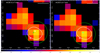Fig. 1. Left panel: nuclear region of 3C 187 as imaged by Chandra-ACIS detector in the 0.3 − 7 keV band, smoothed with a Gaussian kernel with a 1 × 1 pixel ($0\stackrel{″}{.}492\times 0\stackrel{″}{.}492$) σ. The white diamond indicates the optical identification by Hes et al. (1995), and the green cross indicates the radio core position by Neff et al. (1995). The white line represents the 1 mJy beam−1 contour of the VLA 4.87 GHz observation presented by Bogers et al. (1994). The white X indicates the position of the centroid evaluated in the region represented with the green dashed line. Right panel: same as the left panel after the registration of the X-ray image to match the centroid position with radio core position.

3.1. X-ray extended emission

We produced full 0.3 − 7 keV, soft (0.3 − 3 keV), and hard (3 − 7 keV) band images of Chandra data centered on ACIS-S chip 7. We also produced point spread function (PSF) maps (with the MKPSFMAP task), effective area corrected exposure maps, and flux maps using the FLUX_OBS task.

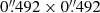
In Fig. 2 we present a comparison of the central ∼3′ region of 3C 187 as seen in the VLA 1.4 GHz (20 cm) map (upper left panel) and in the full (upper right panel), soft (lower left panel), and hard (lower right panel) X-ray flux maps. We can clearly see that the X-ray emission appears elongated in the same direction of the radio lobes; enhanced emission extends up to the lobes themselves. In addition, we see that X-ray emission above 3 keV is essentially compatible with the background, and therefore in the following we only consider Chandra images in the soft 0.3 − 3 keV energy range.

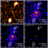Fig. 2. Upper left panel: archival VLA 1.4 GHz (20 cm) image of the central ∼3′ region of 3C 187 (Neff et al. 1995) obtained via AIPS standard reduction procedure (http://www.aips.nrao.edu/cook.html). The clean beam (shown in the lower left with a cyan ellipse) is 3″ × 3″ with major axis P.A. = 0°, and the rms noise is 87.3 μJy per beam. The green circles represent the locations of the north and south lobe peaks as reported by Rhee et al. (1996), while the green cross denotes the peak of the core emission as seen in the 6 cm map (Neff et al. 1995). Upper right panel: full band 0.3 − 7 keV ACIS-S flux image smoothed with a Gaussian kernel with a 5 × 5 pixel ($2\stackrel{″}{.}46\times 2\stackrel{″}{.}46$) σ, with superimposed in white VLA L-band contours from the left panel image. The radio contours start at 30 times the rms level, increasing by factors of four. The sources indicated in this panel are the same as the right panel. Lower left and right panels: same as the upper right panel, but in the 0.3 − 3 keV and 3 − 7 keV bands.

In Fig. 3 we compare the inner ∼5′ region of 3C 187 as imaged by the GMRT 150 MHz map (left panel) collected during the TIFR GMRT Sky Survey (TGSS; Intema et al. 2017), and in the soft X-ray flux map (right panel). For comparison, we overlay on the latter both the VLA 1.4 GHz and the GMRT 150 MHz contours. Again, the soft X-ray emission is elongated in the direction of the radio lobes as seen in the GMRT map and most of the emission lies between these lobes.

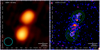Fig. 3. Left panel: archival GMRT 150 MHz image (http://tgssadr.strw.leidenuniv.nl/doku.php) of the central ∼5′ of 3C 187 obtained from the TGSS survey. The clean beam (shown in the lower left with a cyan ellipse) is $26\stackrel{″}{.}5\times 25″$ with major axis P.A. = 0°), and the rms noise is 2.6 mJy per beam. Right panel: soft band 0.3 − 3 keV ACIS-S flux image smoothed with a Gaussian kernel with a 5 × 5 pixel ($2\stackrel{″}{.}46\times 2\stackrel{″}{.}46$) σ, with superimposed in white VLA L band contours from the upper right panel of Fig. 2, while the green lines represent the GMRT 150 MHz contours starting at 30 times the rms level, increasing by factors of four.

To define regions of cone (along the radio axis) and cross-cone (perpendicular to the radio axis) emission we produced a 0.3 − 3 keV azimuthal surface flux profile, extracting data in angular sectors centered on the brightest pixel shown in the left panel of Fig. 1, with an inner and outer radii of 2″ and 100″ and an arbitrary width of 15° (as shown in the left panel of Fig. 4), excluding counts from detected point-like sources. We then fit the obtained profile with a model comprising two Gaussian functions, plus a constant to take into account the background level, as shown in the right panel of Fig. 4. This allows us to identify two cone regions with the angles comprised between two standard deviations from each Gaussian peak. Thus the north (N) cone is centered at a P.A. −13.3° and ranges between −42.1° and 15.5°, while the south (S) cone is centered at a P.A. 164.0° and lies between 128.7° and 199.3° as shown in Fig. 5. We note that varying the angular sector width between 10° and 20° has little effect on the estimate of the cone regions.

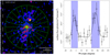Fig. 4. Left panel: soft band 0.3 − 3 keV ACIS-S flux image smoothed with a Gaussian kernel with a 5 × 5 pixel ($2\stackrel{″}{.}46\times 2\stackrel{″}{.}46$) σ, with the angular sectors used for the azimuthal profile extraction superimposed in green. Right panel: black points indicate the surface flux profile in the 0.3 − 3 keV band extracted in the sectors shown in the left panel; the vertical black bars indicate the uncertainties on the surface flux and the horizontal black bars indicate the bin widths. The full black line represents the best-fit model, comprising two Gaussians plus a constant to account for the background level, for the profile; the blue shaded areas represent the regions chosen for the N and S cone regions, that is, the angles comprised between two standard deviations from each Gaussian peak.

We made use of the standard beta model (Cavaliere & Fusco-Femiano 1976, 1978) to investigate the presence of enhanced X-ray emission in these regions; this model is generally used to fit the surface brightness profile in relaxed galaxies or groups and clusters of galaxies,

$$\begin{array}{c}\hfill S_b(r)=S_0{\left[1+{\left(\frac{r}{r_C}\right)}^2\right]}^{1/2-3\beta },\end{array}$$(2)

where S₀ is the central surface brightness, r_C is the core radius, and β is linked to the projected galaxy velocity dispersion σ_R and gas temperature T by $\beta =\mu m_{\text{H}}{\sigma }_R{}^2/kT$ (where μ is the mean molecular weight, m_H is the mass of the hydrogen atom, and k is the Boltzmann constant). As mentioned before, when fitting a surface flux profile rather than a surface brightness profile with a beta model the only difference is the S₀ parameter, which would yield the central surface flux instead of the central surface brightness.

Then, to evaluate the extension of the emission in the cones and cross-cone direction we extracted net surface flux profiles in the directions presented in Fig. 5, excluding counts from detected sources, and extracting the background from source-free regions of chip 7 and 6. The width of the bins was adaptively determined to reach a minimum signal-to-noise ratio of 3. In the outer regions, when this ratio could not be reached, we extended the bin width up ∼200″ from the nucleus.

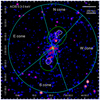Fig. 5. Soft band 0.3 − 3 keV ACIS-S flux image smoothed with a Gaussian kernel with a 5 × 5 pixel ($2\stackrel{″}{.}46\times 2\stackrel{″}{.}46$) σ, with the cone regions defined in Fig. 4 superimposed in cyan. The white and green lines represent the contour level at 30 times the rms level for the VLA 1.4 GHz (see Fig. 2) and GMRT 150 MHz (see Fig. 3) maps, while the magenta xs represent the detected X-ray sources.

Surface flux profiles in the cross-cone, N, S direction are presented in Fig. 6. The best-fit beta models are shown with dashed lines, and residuals to these models are presented on the bottom of each panel. The best-fit parameters for these profiles are reported in Table 1.

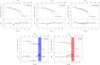Fig. 6. Surface flux profiles in the 0.3 − 3 keV band extracted in the E cone (upper left panel), W cone (upper central panel), W+E cone (upper right panel), N cone (lower left panel), and S cone (lower right panel) directions (see Fig. 5). The widths of the bins are adaptively chosen to reach a minimum signal-to-noise ratio of 3. Upper limits are indicated with downward triangles. For the upper panels the dashed black lines represent the best-fit beta model the profiles. For the lower panels, the black dashed lines represent the best-fit beta model to the E+W cone, normalized to match the first bin. The vertical green dashed lines indicate the locations of the contour level at 30 times the rms level for 150 MHz map, while the colored vertical areas denote the locations of the contour level at 30 times the rms level for the VLA 1.4 GHz (see Fig. 5). The colored dashed lines represent the best-fit beta model the profiles, excluding the bins in the colored vertical area. The residuals to such fits are indicated at the bottom of each panel.

We see that the soft X-ray emission extends with a signal-to-noise ratio of at least 3 up to ∼45″ (corresponding to ∼270 kpc) both in the W (upper left panel) and E (upper central panel) directions, respectively. The best-fit beta models are shown with black dashed lines. The best-fit parameters for the beta model are r_C = 115 ± 46 kpc and β = 0.83 ± 0.31 for the W direction, and r_C = 98 ± 4 kpc and β = 0.73 ± 0.03 for the E direction. Considering the uncertainties, which are larger for the W direction, the two profiles are compatible. In addition we extracted a combined surface flux profile in the W and E direction (upper right panel). For this combined profile, we get best-fit parameters of r_C = 142 ± 55 kpc and β = 0.85 ± 0.37. Although the uncertainties for this combined profile are larger than for the W and E directions, possibly resulting from the mixture of gas with a different distribution, this is useful to characterize the average profile away from the enhanced emission in the direction of the radio lobes.

In the lower panels of Fig. 6 we present surface flux profiles for the N and S direction. The soft X-ray emission extends with a signal-to-noise ratio of at least 3 up to ∼75″ (corresponding to ∼450 kpc) and ∼70″ (corresponding to ∼400 kpc) in the N (lower left panel) and S (lower right panel) directions, respectively. In both directions, the surface flux signal-to-noise ratio drops below 3 just after the radio lobe regions. In these panels we indicate the locations of the contour level at 30 times the rms level for the 150 MHz and VLA 1.4 GHz maps (see Fig. 5). The colored dashed lines represent the best-fit beta models to surface flux profiles with the exclusion of the bins falling in the colored areas, which are likely to contain enhanced X-ray flux with respect to a diffuse thermal emission described by a beta model. For the N cone the best-fit r_C = 185 kpc is essentially unconstrained, while for the β parameter we obtain β = 0.69  ±  0.30. For the S cone instead we obtain r_C = 292  ±  9 kpc and β = 0.84  ±  0.02. These results suggest that the soft X-ray emission is significantly more extended in the S cone than in the N cone. Looking at the residuals at the bottom of each panel, we see that positive residuals tend to fall in correspondence with the colored areas that denote the VLA 1.4 GHz radio emission and this is more significant in the N cone.

We also tried comparing the observed surface flux profiles in the N and S cones with that observed in the cross-cone direction. To this end, we plotted the best-fit beta model obtained in the W+E cones, normalizing it to match the first bin of the N and S surface flux profiles in the lower panels of Fig. 6. We see that the surface flux profile is above that observed in the cross-cone directions at R ≳ 200 kpc in the N cone and at all radii in the S cone. This suggests that either the thermal emission in N and S cone is more extended than in the cross-cone direction or that there is additional emission on top of the thermal emission in correspondence with the radio lobes, extending in the S cone closer to the nucleus than what we observe in the N cone.

In conclusion, the X-ray emission from 3C 187 appears extended in all directions, more in the N and S cone than in the cross cone, and that it is generally compatible with a beta model distribution, with enhanced emission coincident with the radio lobes, in particular the N cone. The best-fit β values in the W, E, S, and N cones are ∼0.8, ∼0.7, ∼0.8, and ∼0.6, although this parameter is poorly constrained. Such values are similar to those observed in groups and clusters of galaxies (Mulchaey et al. 1996; Mohr et al. 1999; Helsdon & Ponman 2000). For the N and S cone, we see enhanced emission with respect to the cross-cone in correspondence with the radio lobes. This suggests the possibility of a significant contribution to the observed X-ray flux by the nonthermal process (see Sect. 4.1), in which case beta models do not necessarily describe the underlying gravitational potential.

3.2. X-ray spectral analysis

We extracted spectra in the regions presented in Fig. 7 on the basis of the surface flux profiles shown in Fig. 6. Since the N and S lobes almost completely encompass N and S cone regions as defined above (see Fig. 7), we decided to extract spectra in the lobes to represent the regions of enhanced radio emission. We also extracted a spectrum in the cross-cone region by combining the W and E direction and excluding the overlapping regions covered by the N and S lobes.

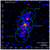Fig. 7. Soft band 0.3 − 3 keV ACIS-S flux image smoothed with a Gaussian kernel with a 5 × 5 pixel ($2\stackrel{″}{.}46\times 2\stackrel{″}{.}46$) σ, with superimposed the regions used for spectral extraction. The cyan lines (full for the cross-cone directions and dashed for the N and S directions) represent the cones in which the soft X-ray emission extends with a signal-to-noise ratio of at least 3 (see Fig. 6). The green lines represent the contour level at 30 times the rms level for the 150 MHz (see Fig. 3) maps. The magenta xs represent the detected X-ray sources, excluded from the spectral extraction.

We produced spectral response matrices weighted by the count distribution within the aperture (as appropriate for extended sources). Background spectra were extracted in the same source-free regions used for radial profile extraction (Sect. 3.1).

Firstly, we subtracted background spectra from source spectra, making use of the χ² fit statistic and binning the spectra to obtain a minimum of 30 counts per bin. Spectral fitting was performed in the 0.3 − 7 keV energy range with the SHERPA application (Freeman et al. 2001) via three different models: a simple power law (POWERLAW), which should represent the IC/CMB emission in the nonthermal scenario; a thermal plasma (XSAPEC⁶) with C, N, O, Ne, Mg, Al, Si, S, Ar, Ca, Fe, and Ni abundances fixed to solar values, which should model the emission from the IGM; and a model that comprises both the power law and the thermal plasma. In all the models we included photo-electric absorption by the Galactic column density along the line of sight N_H = 6.36 × 10²⁰ cm⁻² (HI4PI Collaboration 2016). The results of these fits are presented in Table 2 and in Fig. 8. Errors correspond to the 1σ confidence level for one interesting parameter (Δχ² = 1). We also tried modeling the extracted spectra with a XSVAPEC model using variable element abundances. This model, however, yielded unconstrained abundances and had fit statistics and temperatures similar to the fixed abundance model.

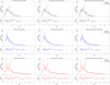Fig. 8. Spectral fits in the 0.3 − 7 keV band performed with a thermal XSAPEC (left column), power-law (central column), and mixed thermal+power-law (right column) models. From top to bottom we show spectra extracted in the cross cone, N lobe, and S lobe regions. In upper portion of each panel the full line represents the best-fit model and the crosses represent the data points, while the residual distribution is presented in the lower portion of each panel. For the thermal+power-law model (right column), the dotted line represents the thermal component, the dashed line represents the power-law component, and the full line represents the total model.

In the cross-cones direction the power-law model (upper left panel of Fig. 8) yields a photon index Γ = 1.9 ± 0.3, while the thermal plasma model (upper central panel) yields a poorly constrained temperature $kT={3.9}_{-1.2}^{+2.6}\mathrm{keV}$; the two models give similar reduced χ² values. When applying the mixed power-law+thermal model, the power-law component is poorly constrained, and its photon index and normalization were therefore fixed to their best-fit values, obtaining a reduced χ² similar to the previous models. The best-fit thermal component has a temperature $kT={3.3}_{-1.0}^{+1.9}\mathrm{keV}$, which is compatible with the temperature evaluated with the thermal model alone, and as shown in the upper right panel of Fig. 8, it appears to be dominant with respect to the power-law component, which contributes to ∼9% of the total flux. We cannot however rule out either the thermal or the nonthermal model on a statistical base.

In the N lobe region the power-law model (central left panel) yields a photon index Γ = 2.3 ± 0.3, while the thermal model (central panel) yields a temperature $kT={2.7}_{-0.7}^{+1.1}\mathrm{keV}$, again with similar reduced χ² values. When applying the mixed power-law+thermal model, we fixed the temperature of the thermal component to the best-fit value obtained in the cross-cone region to check for the presence of the same hot plasma in the N lobe region. The resulting normalization of the thermal component resulted poorly constrained, so we fixed it to its best-fit value and obtained a reduced χ² similar to the previous models. The best-fit power-law component has a photon index 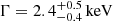$\mathrm{\Gamma }={2.4}_{-0.4}^{+0.5}\mathrm{keV}$, which is compatible with the photon index evaluated with the power-law model alone; as shown in the central right panel, this component appears to be dominant with respect to the thermal component, which however contributes to ∼20% of the total flux. Again, we cannot rule out either the thermal or the nonthermal model on a statistical basis.

In the S lobe the power-law model yields a photon index Γ = 1.8 ± 0.3 with a reduced χ² = 1.04, while the thermal model yields an unconstrained temperature 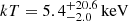$kT={5.4}_{-2.0}^{+20.6}\mathrm{keV}$ with a reduced χ² = 1.16. This suggests that in this region the power-law model is statistically favored. The mixed model with the temperature of the thermal component fixed to the value obtained in the cross-cone region yields a zero normalization for the thermal component. The mixed model is therefore equivalent to the power-law model, indicating that X-ray emission in the S lobe is mainly of nonthermal origin.

We then repeated the spectral fits described above, but instead of subtracting the background spectra we modeled them using the prescription given by Markevitch et al. (2003); that is, a model comprising a thermal plasma component (MEKAL; Kaastra 1992) with solar abundances and a power law. For this analysis we binned the spectra to obtain a minimum of 1 count per bin, making use of the cash statistic. The results of these fits are presented in Table 3.

The best-fit parameters obtained in this way are compatible with those obtained subtracting the background spectra. However, owing to the increased statistic, these parameters are better constrained with smaller uncertainties, with the exception of the temperature in the S lobe region, which is even less constrained in this case. Another difference with respect to the previous analysis is the fit with the mixed model (power-law+thermal) in the N lobe region, where the thermal component with the temperature fixed to the value obtained in the cross-cone region yields a zero normalization, reinforcing the scenario of a dominating nonthermal emission from this region.

We note that the intrinsic (i.e., unabsorbed) X-ray luminosities L_0.5−2 ≈ 3 × 10⁴³ erg s⁻¹ inferred from the thermal models are compatible within the scatter with those expected from the L_X − T relation observed in clusters (Markevitch 1998, their Fig. 1; Zou et al. 2016, their Fig. 2) in the N lobe and cross-cone region, while in the S cone the luminosity is significantly lower than those expected from thermal emission from thermal gas at a temperature of ∼5 keV. In addition, we note that the photon indices obtained with the power-law models are similar to those observed in lobes X-ray detected from other radio galaxies (Croston et al. 2005).

In conclusion, although we cannot rule out either the thermal or the nonthermal model with the statistics of the present data, we consider the former to be favored in the cross-cone region to explain the observed X-ray emission. The spectral fit results suggest that the X-ray emission form the N lobe is mainly due to nonthermal processes, in which the presence of a hot thermal plasma contributes up to ∼20% of the observed flux. In the S lobe, on the other hand, a purely nonthermal emission is the favored interpretation for the observed X-ray radiation. A significant contribution from thermal emission from hot IGM in either lobe however cannot be ruled out. As a matter of fact, disentangling the origin of X-ray radiation between thermal radiation and IC/CMB emission by only comparing fit statistic has proven to be challenging even with larger statistics, for example, a larger number of counts (see, e.g., Hardcastle & Croston 2010); thus additional data are needed to draw firmer conclusions on the spectral analysis of 3C 187.

4. Discussion

4.1. Nonthermal scenario: IC/CMB emission

To investigate the nature of the observed X-ray structure and its connection with the radio emission, in this section we study the multiwavelength properties of 3C 187 and try to interpret these properties in the IC/CMB scenario.

We made use of the VLA L-band map at 1.4 GHz (upper left panel of Fig. 2) and the GMRT map at 150 MHz (left panel of Fig. 3). For both images we measured the flux densities in the regions of N and S lobes by the contour level at 30 times the rms level for the GMRT map (see Fig. 3), obtaining flux densities similar to those of the literature (Neff et al. 1995; Rhee et al. 1996).

For the X-ray emission, we made use of the spectra extracted in the N and S lobes presented in Fig. 8 convolved with the response function to obtain flux measurements. In particular, since we want to test the nonthermal scenario, for the N lobe we used the power-law component of the mixed model (center right panel of Fig. 8), while for the S lobe we used the power-law model since it is equivalent to the mixed model.

To model the multiwavelength emission of 3C 187 we used the Jets Spectral Energy Density (SED) modeler and fitting Tool (JetSeT⁷; Tramacere et al. 2009, 2011) to simulate single-zone synchrotron and IC/CMB emissions in the lobes. For both lobes we adopted an electron energy distribution in the form of a power law n(γ)∝γ^−p extending between a minimum and maximum energy γ_min and γ_max so that

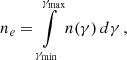$$\begin{array}{c}\hfill n_e={\displaystyle \underset{{\gamma }_{\min }}{\overset{{\gamma }_{\max }}{\int }}n(\gamma )d\gamma ,}\end{array}$$(3)

where n_e is the electron number density.

We approximated the N lobe with an ellipsoid with semiaxis r_l = 46″ along the radio P.A. and r_w = 38″ across it (the semiaxis along the line of sight is taken equal to r_w) following the radio contours at 150 MHz. Similarly, we approximated the S radio lobe as an ellipsoid with r_l = 50″ and r_w = 38″. This yields an equivalent spherical radius $R=\sqrt[3]{r_l{r_{\mathit{w}}}^2}$ of 240 kpc and 247 kpc for the N and S lobe, respectively, which was fixed during the fit. During the fit we assumed, γ_min = 10, γ_max = 10⁵, a bulk Lorentz factor of 1 and a viewing angle of 90°. The free parameters of the model are therefore the electron energy distribution slope p, the electron density n_e and the magnetic field in the lobe B.

The results of these simulation for the N and S lobe are presented in Fig. 9 using the spectral energy distribution (SED; νF_ν) representation, with the full lines representing the synchrotron emission and the dashed lines representing the IC/CMB component. In the same figure we overplot the radio fluxes at their relative frequency, while for the X-ray fluxes we use “butterfly” plots to represent the corresponding spectral indices obtained from the lobe fittings, centered at the geometric average of 0.3 and 7 keV. The full line butterflies represent the spectral indices obtained with the background subtraction (see Table 2), while the dot-dashed butterflies represent the spectral indices obtained with the background modeling (see Table 3). The parameters used for reproducing the observed SED are presented in Table 4, together with the calculated total radiative luminosity L_rad (that is, the combined luminosity from synchrotron and IC/CMB radiation) and with the total electron energy 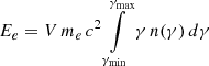$E_e=V{m}_e{c}^2\underset{{\gamma }_{\min }}{\overset{{\gamma }_{\max }}{\int }}\gamma n(\gamma )d\gamma$, where V is the emitting region volume and m_e is the electron mass. We note that similar values of E_e can be evaluated with the method presented in Erlund et al. (2006). We also note that the magnetic field values obtained from the fits are similar to the equipartition value of ∼7 μG.

Fig. 9. Observed SED (νFν) of N (in blue) and S (in red) lobes of 3C 187. Squares represent GMRT fluxes and diamonds represent VLA fluxes. The butterflies indicate the uncertainties on the spectral indices obtained from the power-law fits in the lobes (see Sect. 4.1). The full line butterflies represent the spectral indices obtained with the background subtraction, while the dot-dashed butterflies represent the spectral indices obtained with the background modeling. The full lines represent the simulation of the synchrotron emission, while the dashed lines represent the IC/CMB emission in the same region. The vertical dotted line marks the frequency (∼4 MHz) obtained from Eq. (1) at which the electrons responsible for the IC/CMB radiation at 1 keV emit synchrotron radiation given the magnetic field values shown in Table 4.

As shown in Fig. 9 the observed X-ray spectral slope in the radio lobes of 3C 187 is compatible (although marginally) with the scenario of the X-ray emission, which is due to IC/CMB radiation from the same electron population responsible for the synchrotron emission we observe at radio frequencies.

By comparing total electron energy E_e and the radiative luminosity L_rad, we can estimate the radiative cooling time τ = E_e/L_rad as τ ≃ 2.0 × 10¹⁰ yr and τ ≃ 1.8 × 10¹⁰ yr for the N and S lobe, respectively. The electrons in lobes would therefore loose their energy through radiative emission on spatial scales ∼6 Gpc, far larger than the size of the observed radio structures (∼250 kpc). In conclusion, the X-ray radiation from the radio lobes of 3C 187 can be explained in terms of nonthermal radiation, namely IC/CMB, with a population of energetic electrons capable of emitting the observed fluxes over tens of Gyr.

4.2. Thermal scenario: Hot gas in the IGM

Since the spectral analysis presented in Sect. 3.2 does not rule out the possibility that the diffuse X-ray emission from 3C 187 originates from IGM hot plasma, in this section we examine the implications of this scenario. To this end, we make use of the spectra presented in Sect. 3.2, in particular those obtained with the thermal XSAPEC model; that is, we assume that the observed X-ray emission is entirely due to thermal gas (left column of Fig. 8).

From the normalization of the XSAPEC models (i.e., their emission measures EM), we can evaluate the gas proton density n_H in the lobes. Assuming a uniform particle density in the emitting region we have

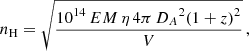$$\begin{array}{c}\hfill n_{\mathrm{H}}=\sqrt{\frac{{10}^{14}EM\eta 4\pi {D_A}^2{\left(1+z\right)}^2}{V}},\end{array}$$(4)

where D_A is the angular distance of the source, V is the emitting region volume, and η ≈ 0.82 is the ratio of proton to electron density in a fully ionized plasma. Neglecting the electron density, which contributes to the total gas density less than ∼7 × 10⁻⁴, we can estimate the thermal energy of the gas as $E_{\mathrm{therm}}=\frac{3kT{n}_{\mathrm{H}}V}{2\mu }$, where k is the Boltzmann constant, T is the gas temperature, and μ ≈ 0.62 is the mean particle weight in units of the proton mass.

Approximating the N and S lobes with the same ellipsoids defined in Sect. 4.1 we obtain $E_{\mathrm{therm},\mathrm{N}}={2.5}_{-0.8}^{+1.2}\times {10}^{61}\mathrm{erg}$ and $E_{\mathrm{therm},\mathrm{S}}={5.3}_{-2.3}^{+20.7}\times {10}^{61}\mathrm{erg}$. The sound-speed expansion time 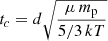$t_c=d\sqrt{\frac{\mu m_{\mathrm{p}}}{5/3kT}}$, where m_p is the proton mass and d is the distance of the center of the lobes from the source nucleus, evaluated as t_cs, N = 0.4 ± 0.1 Gyr and 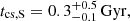$t_{\mathrm{cs},\mathrm{S}}={0.3}_{-0.1}^{+0.5}\mathrm{Gyr},$ respectively, yields thermal powers L_therm = E_therm/t_cs of $L_{\mathrm{therm},\mathrm{N}}={2.1}_{-0.7}^{+1.1}\times {10}^{45}\mathrm{erg}{\mathrm{s}}^{-1}$ and $L_{\mathrm{therm},\mathrm{S}}={6.3}_{-2.9}^{+27.5}\times {10}^{45}\mathrm{erg}{\mathrm{s}}^{-1}$, which are ∼30 and ∼80 times larger than the X-ray luminosities estimated from the spectral fitting. In fact, we can estimate the X-ray cooling time as τ = E_therm/L_X as τ_N = 12 Gyr and τ_S = 21 Gyr for the N and S lobe, respectively, indicating that only a small fraction of the thermal energy contained in the lobes is emitted as X-ray radiation, allowing them to shine over long times. Using the fit results obtained from background spectra modeling in the N lobe region, we obtain similar results of 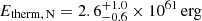$E_{\mathrm{therm},\mathrm{N}}={2.6}_{-0.6}^{+1.0}\times {10}^{61}\mathrm{erg}$, $L_{\mathrm{therm},\mathrm{N}}={2.3}_{-0.6}^{+0.9}\times {10}^{45}\mathrm{erg}{\mathrm{s}}^{-1}$, and τ_N = 14 Gyr. Since the background spectra modeling in the S lobe region yields poorly constrained, out of the band temperature, we do not consider this modeling for these estimates.

As an additional test of the thermal origin for the diffuse X-ray emission in the lobes of 3C 187, we check if the gas in these regions happens to be in pressure equilibrium with the surrounding environment (i.e., P ≃ P_IGM), so that the IGM could contain the gas located in the lobes (Hardcastle et al. 2002, 2004). The thermal pressure of the gas can be estimated as $P=\frac{n_{\mathrm{H}}kT}{\mu }$. Approximating the cross-cone region as a double three-dimensional cone, we obtain in this region a gas pressure 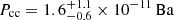$P_{\mathrm{cc}}={1.6}_{-0.6}^{+1.1}\times {10}^{-11}\mathrm{Ba}$; in the N and S lobe, we obtain $P_{\mathrm{N}}={1.0}_{-0.3}^{+0.5}\times {10}^{-11}\mathrm{Ba}$ and $P_{\mathrm{S}}={1.9}_{-0.8}^{+7.5}\times {10}^{-11}\mathrm{Ba}$, respectively. Again, considering the fits with background spectra modeling, we similarly obtain $P_{\mathrm{cc}}={1.3}_{-0.3}^{+0.4}\times {10}^{-11}\mathrm{Ba}$ in the cross-cones, while in the N lobe we obtain $P_{\mathrm{N}}={1.0}_{-0.2}^{+0.4}\times {10}^{-11}\mathrm{Ba}$. If we assume P_IGM = P_cc, the gas thermal pressure in the lobes is compatible within the uncertainties with the pressure of the surrounding gas, indicating that the former would be contained by the latter.

In conclusion, X-ray radiation in the radio lobes of 3C 187 can be interpreted as due to thermal emission from hot gas with temperatures of ∼3 keV and ∼5 keV in the N and S lobes, respectively. The cooling times indicate that the thermal gas contained in the radio lobes emits a small fraction of its thermal energy in the form of X-ray radiation, allowing this gas to shine in over tens of Gyr. In addition, the X-ray emitting thermal gas in radio lobes would be in pressure equilibrium with the surroundings, thus preventing expansion of this gas.

4.3. Cluster analysis

As previously mentioned, Hutchings et al. (1988) and Neff et al. (1995) reported that 3C 187 appears to be a member of a cluster of ∼30 objects projected between the radio lobes. To check if this source resides in a cluster of galaxies that could account for the extended emission we see in the Chandra images, we checked for the presence of a red sequence in the source field because there is no redshift measurement available for sources in the field of 3C 187, apart from the source itself. The red sequence in the form of a tight clustering of the galaxies in the color space (Visvanathan & Sandage 1977; Annis et al. 1999) provides an efficient method to detect clusters (e.g., Blakeslee et al. 2003; Mullis et al. 2005; De Lucia et al. 2007).

We collected photometrical data in the field of 3C 187 from the Pan-STARRS Data Release 2 (DR2, Flewelling 2018), namely g, r, i, z, and y magnitudes for all sources within 2′ (∼700 kpc) from the host galaxy of 3C 187. For this analysis we selected sources detected in all Pan-STARRS filters. In addition, to avoid bright stars, we restricted our selection to sources with magnitudes larger than 14 and considered only sources with magnitude errors smaller than 10%, thereby obtaining a sample of 200 sources. We also collected ∼50⁵ sources in random positions of the sky, selected in the same way as for the sources in 3C 187 field. We then de-reddened the observed magnitudes of each source using the measurements of dust reddening by Schlafly & Finkbeiner (2011) and the extinction model of Fitzpatrick & Massa (2007).

To verify and confirm the existence of a red sequence in 3C 187 field, we followed a procedure similar to those presented in Lu et al. (2009) and Hao et al. (2009). Following Murphy et al. (2012), we investigated the presence of red sequences in g − r, r − i, i − z and z − y colors. In the upper panels of Fig. 10 we show the normalized distributions of the (de-reddened) colors for random Pan-STARRS sources. We fitted these color distributions with a mixture of Gaussian distributions (using the R package NORMALMIXEM). The best-fit models are overplotted with dashed lines; the best-fit parameters, where μ is the mean value and σ is the standard deviation of the Gaussian, are shown in the legends. We see that the g − m distribution for the random Pan-STARRS sources is adequately represented by the combination of three narrow (σ ≲ 0.2) Gaussians, while for the r − i and i − z distributions we need two Gaussians, one narrow and one wide (σ ∼ 0.5) for r − i and two narrow Gaussians for i − z. Finally the z − y distribution is described by a single narrow Gaussian. We see that the Pan-STARRS counterpart of 3C 187 core is in general redder than the random sources and is fairly separated from these sources in the g − r and z − y representation, while it is less separated in r − i and i − z.

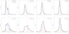Fig. 10. Upper panels: normalized distributions of the (de-reddened) colors for random Pan-STARRS sources. The vertical magenta line denotes the color of the 3C 187 core counterpart. The best-fit Gaussian components are overplotted with dashed lines of different colors, with the best-fit μ and σ indicated in the legend. Lower panels: normalized distributions of the (de-reddened) colors for Pan-STARRS sources in the field of 3C 187. As in the upper panels, the vertical magenta line indicates the color of the 3C 187 core counterpart. The color distributions are modeled with the same Gaussians used to model the random source distribution with fixed μ and σ. The additional component required to model the color distributions is indicated with a red dashed line, with the best-fit μ and σ indicated in the legend. The g − r and z − y colors require a further broad, subdominant component indicated with a green dashed line.

In the lower panels of Fig. 10 we show the normalized distributions of the (de-reddened) colors for Pan-STARRS sources found in a circle within 2 arcmin around the core of 3C 187. We modeled these distributions with the same Gaussians found in the color distributions of the random sources (keeping fixed their μ and σ), plus one or two additional Gaussian that should describe the (non-background/foreground) sources around 3C 187. These are usually described by a narrow Gaussian centered around the colors of the 3C 187 core counterpart, while in the case of g − r and z − y we also find a broad, subdominant component.

Following Hao et al. (2009), we considered the sources lying between two σ around the mean value of the narrow (red) component to select our bona fide cluster members among the Pan-STARRS sources in the field of 3C 187. In addition, to exclude contamination for background/foreground sources (that can be significant in r − i and i − z colors) we excluded the sources up to one σ from the mean value of the redder component of the random sources. As expected, this resulted in no selected sources for the r − i color, while we were able to select 40, 42, and 60 sources for g − r, i − z and z − y, respectively, including the counterpart of 3C 187 core. Since we do not assume that 3C 187 is necessarily the brightest source in the group, we further selected sources up to one magnitude fainter than the Pan-STARRS counterpart of the 3C 187 core, resulting in a final sample of 39, 41, and 57 sources for g − r, i − z, and z − y color, respectively. A Kolmogorov–Smirnov test (Kolmogorov 1933; Smirnov 1939) shows that the distributions of the Pan-STARRS colors cluster member candidates have p-chances < 10⁻¹⁵ of having been randomly sampled from the population of random sources.

In Fig. 11 we show the Pan-STARRS sources in 3C 187 field in the color-magnitude space g − r versus r, i − z versus z, and z − y versus y in the left, central, and right panels, respectively. The red dashed lines show a linear fit to the cluster member candidates, weighted with the inverse square of the color errors. We obtain best-fit slopes of 0.08 ± 0.03, −0.03 ± 0.02, and 0.06 ± 0.01 and 90% scatters of 0.21, 0.15, and 0.15 for the g − r, i − z, and z − y colors, respectively, which are represented with black dashed lines.

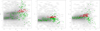Fig. 11. Pan-STARRS sources in the field of 3C 187 presented in the color-magnitude space. The cluster member candidates are reported with red circles, the other field sources are represented with green circles, and sources from random positions in the sky are plotted in the background with gray dots. The counterpart of 3C 187 core is represented with a magenta circle. The red dashed lines show a linear fit to the selected cluster member candidates, while 90% scatters are represented with black dashed lines.

In Fig. 12 we show the locations of the Pan-STARRS sources selected as cluster member candidates in celestial coordinates, on top of the Pan-STARRS images of 3C 187 in different filters. The red circles indicate the cluster member candidates selected in at least one color, while the green circles denote the field sources not selected as cluster member candidates selected in any color (field sources hereinafter).

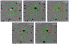Fig. 12. Pan-STARRS images of 3C 187 in the g (upper left panel), r (upper central panel), i (upper right panel), z (lower left panel), and y (lower right panel) filter with the VLA L-band contours superimposed in cyan and in green the GMRT 150 MHz contours. The red circles indicate the cluster member candidates selected in at least one color, while the green circles indicate the field sources not selected as cluster member candidates in any color. The magenta circle indicates the counterpart to 3C 187 core, and the white diamond indicates the location of the optical identification by Hes et al. (1995) for the 3C 187 nucleus. White crosses represent X-ray point sources detected in the 0.3 − 7 keV Chandra image. The xs indicate the sources for which optical spectra were obtained with Victor Blanco Telescope. In particular, the green xs indicates sources with stellar spectra and the red x indicates the source with a galactic spectrum with redshift 0.4662 (see Fig. 13).

From this image we can clearly see that the cluster member candidates are very dim in the optical, and the core of 3C 187 has a Pan-STARRS magnitude r = 21.0. On the other hand, the brightest optical source in the field is located at RA = 07h45m03s.482, $\mathrm{Dec}=+02{}^{°}00\prime 41\stackrel{″}{.}15$ with Pan-STARRS magnitude r = 12.1. This is coincident with the 2MASS source J07450348+0200411 and an X-ray point source detected in 0.3 − 7 keV Chandra image with a flux of ${0.99}_{-0.33}^{+0.42}\times {10}^{-14}\mathrm{erg}{\mathrm{cm}}^{-2}{\mathrm{s}}^{-1}$, which is the brightest X-ray source detected in the central 2′ around 3C 187.

To investigate the nature of the sources in the field of 3C 187 and verify if they are gravitationally bound, we performed optical spectroscopic observations of sources in the field of 3CR 187, adopting a similar procedure to that carried out for 3CR 17 (Madrid et al. 2018). We acquired spectral images at Victor Blanco 4 m Telescope in Cerro Tololo, Chile on March 10–11 2020, in remote mode. We used the COSMOS spectrograph, which has a field of view of 10′ and a scale of $0\stackrel{″}{.}29$ per pixel. We made use of multi-object slit mode, using the Red VPH Grism (r2k) for three masks with $1\stackrel{″}{.}2$ slit width per source. We integrated each mask three times, with 1200 s per exposition. We acquired Hg-Ne-Ar comparison lamp spectra on each target position for the wavelength calibration. This instrumental setup gave us a spectral coverage of ∼ 5500−9600 Å and dispersion of ∼ 3 Å pixel⁻¹. Additionally, we observed a spectro-photometric standard star for the relative flux calibration (see also Ricci et al. 2015; Landoni et al. 2015; Massaro et al. 2016). Each spectrum was reduced and extracted with standard IRAF procedures (Tody 1986, 1993). Unfortunately, owing to bright night conditions we were able to collect spectra with a signal-to-noise ratio high enough to classify them and obtain a fair redshift estimate for only 23 bright sources in the field of 3C 187 (indicated in Fig. 12 with xs).

In particular we were able to collect spectra for 22 field sources and one cluster member candidate, represented in the figure with green and red xs, respectively. All the field sources showed stellar-like spectra, while the cluster member candidate features a galactic spectrum (shown in Fig. 13) that allowed us to estimate a redshift of 0.466 based on a tentative identification of H, K, Ca I, Hb, and Na I lines. Based on the spectral dispersion of ∼ 3 Å pixel⁻¹ and considering a minimum of two pixels as the minimum resolution for a line, we estimate a redshift uncertainty of 10⁻³. The redshift estimate of 0.466 ± 0.001 for this source is therefore compatible with the redshift of 0.465 reported by Hes et al. (1995) for 3C 187 core, considering a maximum redshift separation Δz = 0.005 (i.e., ∼1500 km s⁻¹) corresponding to the maximum velocity dispersion in groups and clusters of galaxies (see, e.g., Moore et al. 1993; Eke et al. 2004; Berlind et al. 2006)

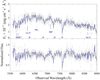Fig. 13. Spectrum of the candidate member for the cluster of 3C 187. Original data points are represented with gray background circles, while the blue line represents the best-fit smoothed model. Some spectral features, H, K, Ca I, Hb, and Na I, are potentially identified at redshift 0.466. The Hα⊙ was also detected as we observed the source during a bright night.

In conclusion, on the basis of Pan-STARRS optical data, the core of 3C 187 belongs to a red-sequence of sources whose color distribution is significantly different from background sources. Optical spectroscopic observations of one cluster member candidate confirm this candidate is at the same redshift as 3C 187 core, while other field sources do not belong to the putative cluster because they are stars. Additional spectroscopic observations aimed at estimating the redshift of cluster member candidates are needed to reveal if they form a gravitationally bound cluster.

5. Summary and conclusions

We performed an imaging and spectral analysis of Chandra data obtained for the radio galaxy 3C 187 in the context of the snapshot program for the 3C catalog (Massaro et al. 2013). In addition to the findings of Massaro et al. 2013, which reported a significant X-ray emission from both the northern and the southern lobes, we preformed an analysis of the surface flux profiles in the N, S, and cross cone directions, extracted X-ray spectra both in the cross cones and in the radio lobe regions, performed a multiwavelength analysis investigating both thermal and nonthermal scenarios for the origin of the diffuse X-ray emission, and investigated the possibility that 3C 187 lies in a cluster of galaxies. The main results of our analysis are as follows:

1. Confirming Massaro et al. (2013) results, we find extended X-ray emission around 3C 187 in all directions. In particular, in the soft 0.3 − 3 keV band the emission is extended ∼850 kpc along the radio lobe direction with a signal-to-noise ratio of at least 3, while this extension reaches ∼530 kpc in the cross-cone direction. The surface flux profiles in the different directions are generally compatible with a beta model, although enhanced emission appears in correspondence with the radio lobes, more prominently in the N cone. The best-fit β values are 0.8, 0.7, 0.7, and 0.8 in the W, E, N, and S cone, respectively, similar to those observed in groups and clusters of galaxies (see, e.g., Xue & Wu 2000; Ettori 2000).

2. The quality of the available spectral data does not allow us to distinguish between a nonthermal scenario, in which the X-ray emission is of nonthermal origin with a spectrum described by a power law, and a thermal scenario, in which the X-ray emission is of thermal origin with a spectrum described by a thermal plasma model. The two spectral models fit the X-ray spectrum extracted in the cross cones and a N lobe with similar reduced χ² values and residual distributions. In the S lobe, however, the thermal model yields a poorly constrained temperature with a reduced χ² ≃ 1.2, while for the power-law model we have χ² ≃ 1.0. Spectral fitting with a double (power-law+thermal) model seems to indicate a dominating thermal emission in the cross-cone region and a dominating nonthermal emission in the lobe regions, with photon indices similar to those observed in other radio galaxies (Croston et al. 2005). Similar results are obtained through modeling of the background spectra.

3. In the nonthermal scenario, through a combined radio-X-ray analysis, we found that the X-ray spectral indices obtained in the lobes are compatible with IC/CMB emission from energetic electrons in these regions capable of emitting the observed fluxes over tens of Gyr.

4. In the thermal scenario, X-ray radiation from the cross-cone region of 3C 187 can be interpreted as due to thermal emission from hot gas with a temperature ∼4 keV. In the N and S cones, we find temperatures ∼3 keV and ∼5 keV, respectively, with cooling times that allow the gas to shine in over tens of Gyr in pressure equilibrium with the surroundings.

5. Using Pan-STARRS optical data, we found that 3C 187 core belongs to a red sequence of ∼40 optical sources in the field. The color distributions of these sources are significantly different from background sources, meaning that 3C 187 could reside in a cluster of galaxies, while not being the brightest one. If this is the case, the diffuse X-ray emission observed around the source could be in part due to thermal radiation from the IGM of such a cluster. To confirm this result, optical spectroscopy will be needed to robustly identify cluster members.

To sum up, the present data yield a complex scenario for 3C 187. The diffuse X-ray emission around the source appears elongated along the radio axis and enhanced in correspondence with the radio lobes, indicating a morphological connection between the emission in the two energy bands. The spectral analysis does not allow us to rule out either the thermal or nonthermal scenarios, although the former seems favored in the cross-cone region and the latter appears dominant in the radio lobe regions. The X-ray spectral indices in the radio lobes are compatible with the IC/CMB scenario, while a thermal gas in these regions would be able to emit over tens of Gyr and in pressure equilibrium with the surroundings. We have some indications that 3C 187 may belong to cluster of galaxies, whose IGM could contribute to the X-ray emission observed around the source. However, deeper X-ray and optical spectroscopic observations are needed to get a clearer picture of this enigmatic source.

Acknowledgments

We thank the anonymous referee for their useful comments and suggestions. This work is supported by the “Departments of Excellence 2018–2022” Grant awarded by the Italian Ministry of Education, University and Research (MIUR) (L. 232/2016). This research has made use of resources provided by the Compagnia di San Paolo for the grant awarded on the BLENV project (S1618_L1_MASF_01) and by the Ministry of Education, Universities and Research for the grant MASF_FFABR_17_01. This investigation is supported by the National Aeronautics and Space Administration (NASA) grants GO9-20083X and GO0-21110X. A.P. acknowledges financial support from the Consorzio Interuniversitario per la Fisica Spaziale (CIS) under the agreement related to the grant MASF_CONTR_FIN_18_02. F. M. acknowledges financial contribution from the agreement ASI-INAF n.2017-14-H.0. A. P. thanks Andrea Tramacere for fruitful discussions. The Pan-STARRS1 Surveys (PS1) have been made possible through contributions of the Institute for Astronomy, the University of Hawaii, the Pan-STARRS Project Office, the Max-Planck Society and its participating institutes, the Max Planck Institute for Astronomy, Heidelberg and the Max Planck Institute for Extraterrestrial Physics, Garching, The Johns Hopkins University, Durham University, the University of Edinburgh, Queen’s University Belfast, the Harvard-Smithsonian Center for Astrophysics, the Las Cumbres Observatory Global Telescope Network Incorporated, the National Central University of Taiwan, the Space Telescope Science Institute, the National Aeronautics and Space Administration under Grant No. NNX08AR22G issued through the Planetary Science Division of the NASA Science Mission Directorate, the National Science Foundation under Grant No. AST-1238877, the University of Maryland, and Eotvos Lorand University (ELTE). This research has made use of data obtained from the Chandra Data Archive. This research has made use of software provided by the Chandra X-ray Center (CXC) in the application packages CIAO, ChIPS, and Sherpa. This research has made use of the TOPCAT software (Taylor 2005).

References

All Tables

All Figures

Fig. 1. Left panel: nuclear region of 3C 187 as imaged by Chandra-ACIS detector in the 0.3 − 7 keV band, smoothed with a Gaussian kernel with a 1 × 1 pixel ($0\stackrel{″}{.}492\times 0\stackrel{″}{.}492$) σ. The white diamond indicates the optical identification by Hes et al. (1995), and the green cross indicates the radio core position by Neff et al. (1995). The white line represents the 1 mJy beam−1 contour of the VLA 4.87 GHz observation presented by Bogers et al. (1994). The white X indicates the position of the centroid evaluated in the region represented with the green dashed line. Right panel: same as the left panel after the registration of the X-ray image to match the centroid position with radio core position.

In the text

Fig. 2. Upper left panel: archival VLA 1.4 GHz (20 cm) image of the central ∼3′ region of 3C 187 (Neff et al. 1995) obtained via AIPS standard reduction procedure (http://www.aips.nrao.edu/cook.html). The clean beam (shown in the lower left with a cyan ellipse) is 3″ × 3″ with major axis P.A. = 0°, and the rms noise is 87.3 μJy per beam. The green circles represent the locations of the north and south lobe peaks as reported by Rhee et al. (1996), while the green cross denotes the peak of the core emission as seen in the 6 cm map (Neff et al. 1995). Upper right panel: full band 0.3 − 7 keV ACIS-S flux image smoothed with a Gaussian kernel with a 5 × 5 pixel ($2\stackrel{″}{.}46\times 2\stackrel{″}{.}46$) σ, with superimposed in white VLA L-band contours from the left panel image. The radio contours start at 30 times the rms level, increasing by factors of four. The sources indicated in this panel are the same as the right panel. Lower left and right panels: same as the upper right panel, but in the 0.3 − 3 keV and 3 − 7 keV bands.

In the text

Fig. 3. Left panel: archival GMRT 150 MHz image (http://tgssadr.strw.leidenuniv.nl/doku.php) of the central ∼5′ of 3C 187 obtained from the TGSS survey. The clean beam (shown in the lower left with a cyan ellipse) is $26\stackrel{″}{.}5\times 25″$ with major axis P.A. = 0°), and the rms noise is 2.6 mJy per beam. Right panel: soft band 0.3 − 3 keV ACIS-S flux image smoothed with a Gaussian kernel with a 5 × 5 pixel ($2\stackrel{″}{.}46\times 2\stackrel{″}{.}46$) σ, with superimposed in white VLA L band contours from the upper right panel of Fig. 2, while the green lines represent the GMRT 150 MHz contours starting at 30 times the rms level, increasing by factors of four.

In the text

Fig. 4. Left panel: soft band 0.3 − 3 keV ACIS-S flux image smoothed with a Gaussian kernel with a 5 × 5 pixel ($2\stackrel{″}{.}46\times 2\stackrel{″}{.}46$) σ, with the angular sectors used for the azimuthal profile extraction superimposed in green. Right panel: black points indicate the surface flux profile in the 0.3 − 3 keV band extracted in the sectors shown in the left panel; the vertical black bars indicate the uncertainties on the surface flux and the horizontal black bars indicate the bin widths. The full black line represents the best-fit model, comprising two Gaussians plus a constant to account for the background level, for the profile; the blue shaded areas represent the regions chosen for the N and S cone regions, that is, the angles comprised between two standard deviations from each Gaussian peak.

In the text

Fig. 5. Soft band 0.3 − 3 keV ACIS-S flux image smoothed with a Gaussian kernel with a 5 × 5 pixel ($2\stackrel{″}{.}46\times 2\stackrel{″}{.}46$) σ, with the cone regions defined in Fig. 4 superimposed in cyan. The white and green lines represent the contour level at 30 times the rms level for the VLA 1.4 GHz (see Fig. 2) and GMRT 150 MHz (see Fig. 3) maps, while the magenta xs represent the detected X-ray sources.

In the text

Fig. 6. Surface flux profiles in the 0.3 − 3 keV band extracted in the E cone (upper left panel), W cone (upper central panel), W+E cone (upper right panel), N cone (lower left panel), and S cone (lower right panel) directions (see Fig. 5). The widths of the bins are adaptively chosen to reach a minimum signal-to-noise ratio of 3. Upper limits are indicated with downward triangles. For the upper panels the dashed black lines represent the best-fit beta model the profiles. For the lower panels, the black dashed lines represent the best-fit beta model to the E+W cone, normalized to match the first bin. The vertical green dashed lines indicate the locations of the contour level at 30 times the rms level for 150 MHz map, while the colored vertical areas denote the locations of the contour level at 30 times the rms level for the VLA 1.4 GHz (see Fig. 5). The colored dashed lines represent the best-fit beta model the profiles, excluding the bins in the colored vertical area. The residuals to such fits are indicated at the bottom of each panel.

In the text

Fig. 7. Soft band 0.3 − 3 keV ACIS-S flux image smoothed with a Gaussian kernel with a 5 × 5 pixel ($2\stackrel{″}{.}46\times 2\stackrel{″}{.}46$) σ, with superimposed the regions used for spectral extraction. The cyan lines (full for the cross-cone directions and dashed for the N and S directions) represent the cones in which the soft X-ray emission extends with a signal-to-noise ratio of at least 3 (see Fig. 6). The green lines represent the contour level at 30 times the rms level for the 150 MHz (see Fig. 3) maps. The magenta xs represent the detected X-ray sources, excluded from the spectral extraction.

In the text

Fig. 8. Spectral fits in the 0.3 − 7 keV band performed with a thermal XSAPEC (left column), power-law (central column), and mixed thermal+power-law (right column) models. From top to bottom we show spectra extracted in the cross cone, N lobe, and S lobe regions. In upper portion of each panel the full line represents the best-fit model and the crosses represent the data points, while the residual distribution is presented in the lower portion of each panel. For the thermal+power-law model (right column), the dotted line represents the thermal component, the dashed line represents the power-law component, and the full line represents the total model.

In the text

Fig. 9. Observed SED (νFν) of N (in blue) and S (in red) lobes of 3C 187. Squares represent GMRT fluxes and diamonds represent VLA fluxes. The butterflies indicate the uncertainties on the spectral indices obtained from the power-law fits in the lobes (see Sect. 4.1). The full line butterflies represent the spectral indices obtained with the background subtraction, while the dot-dashed butterflies represent the spectral indices obtained with the background modeling. The full lines represent the simulation of the synchrotron emission, while the dashed lines represent the IC/CMB emission in the same region. The vertical dotted line marks the frequency (∼4 MHz) obtained from Eq. (1) at which the electrons responsible for the IC/CMB radiation at 1 keV emit synchrotron radiation given the magnetic field values shown in Table 4.

In the text

Fig. 10. Upper panels: normalized distributions of the (de-reddened) colors for random Pan-STARRS sources. The vertical magenta line denotes the color of the 3C 187 core counterpart. The best-fit Gaussian components are overplotted with dashed lines of different colors, with the best-fit μ and σ indicated in the legend. Lower panels: normalized distributions of the (de-reddened) colors for Pan-STARRS sources in the field of 3C 187. As in the upper panels, the vertical magenta line indicates the color of the 3C 187 core counterpart. The color distributions are modeled with the same Gaussians used to model the random source distribution with fixed μ and σ. The additional component required to model the color distributions is indicated with a red dashed line, with the best-fit μ and σ indicated in the legend. The g − r and z − y colors require a further broad, subdominant component indicated with a green dashed line.

In the text

Fig. 11. Pan-STARRS sources in the field of 3C 187 presented in the color-magnitude space. The cluster member candidates are reported with red circles, the other field sources are represented with green circles, and sources from random positions in the sky are plotted in the background with gray dots. The counterpart of 3C 187 core is represented with a magenta circle. The red dashed lines show a linear fit to the selected cluster member candidates, while 90% scatters are represented with black dashed lines.

In the text

Fig. 12. Pan-STARRS images of 3C 187 in the g (upper left panel), r (upper central panel), i (upper right panel), z (lower left panel), and y (lower right panel) filter with the VLA L-band contours superimposed in cyan and in green the GMRT 150 MHz contours. The red circles indicate the cluster member candidates selected in at least one color, while the green circles indicate the field sources not selected as cluster member candidates in any color. The magenta circle indicates the counterpart to 3C 187 core, and the white diamond indicates the location of the optical identification by Hes et al. (1995) for the 3C 187 nucleus. White crosses represent X-ray point sources detected in the 0.3 − 7 keV Chandra image. The xs indicate the sources for which optical spectra were obtained with Victor Blanco Telescope. In particular, the green xs indicates sources with stellar spectra and the red x indicates the source with a galactic spectrum with redshift 0.4662 (see Fig. 13).

In the text

	Fig. 13. Spectrum of the candidate member for the cluster of 3C 187. Original data points are represented with gray background circles, while the blue line represents the best-fit smoothed model. Some spectral features, H, K, Ca I, Hb, and Na I, are potentially identified at redshift 0.466. The Hα⊙ was also detected as we observed the source during a bright night.
In the text

References

- Annis, J., Kent, S., Castander, F., et al. 1999, BAAS, 31, 12.02 [Google Scholar]
- Balmaverde, B., Capetti, A., Grandi, P., et al. 2012, A&A, 545, A143 [NASA ADS] [CrossRef] [EDP Sciences] [Google Scholar]
- Bennett, A. S. 1962, MNRAS, 125, 75 [NASA ADS] [Google Scholar]
- Bennett, C. L., Larson, D., Weiland, J. L., & Hinshaw, G. 2014, ApJ, 794, 135 [NASA ADS] [CrossRef] [Google Scholar]
- Berlind, A. A., Frieman, J., Weinberg, D. H., et al. 2006, ApJS, 167, 1 [NASA ADS] [CrossRef] [Google Scholar]
- Black, A. R. S., Baum, S. A., Leahy, J. P., et al. 1992, MNRAS, 256, 186 [NASA ADS] [Google Scholar]
- Blakeslee, J. P., Franx, M., Postman, M., et al. 2003, ApJ, 596, L143 [NASA ADS] [CrossRef] [Google Scholar]
- Bogers, W. J., Hes, R., Barthel, P. D., et al. 1994, A&AS, 105, 91 [Google Scholar]
- Bowman, J. D., Cairns, I., Kaplan, D. L., et al. 2013, PASA, 30, e031 [NASA ADS] [CrossRef] [Google Scholar]
- Carilli, C. L., Harris, D. E., Pentericci, L., et al. 1998, ApJ, 494, L143 [NASA ADS] [CrossRef] [Google Scholar]
- Cavaliere, A., & Fusco-Femiano, R. 1976, A&A, 500, 95 [NASA ADS] [Google Scholar]
- Cavaliere, A., & Fusco-Femiano, R. 1978, A&A, 70, 677 [NASA ADS] [Google Scholar]
- Celotti, A., & Fabian, A. C. 2004, MNRAS, 353, 523 [NASA ADS] [CrossRef] [Google Scholar]
- Crawford, C. S., & Fabian, A. C. 2003, MNRAS, 339, 1163 [Google Scholar]
- Croston, J. H., Hardcastle, M. J., Harris, D. E., et al. 2005, ApJ, 626, 733 [NASA ADS] [CrossRef] [Google Scholar]
- Dasadia, S., Sun, M., Morandi, A., et al. 2016, MNRAS, 458, 681 [NASA ADS] [CrossRef] [Google Scholar]
- De Lucia, G., Poggianti, B. M., Aragón-Salamanca, A., et al. 2007, MNRAS, 374, 809 [NASA ADS] [CrossRef] [Google Scholar]
- Dewdney, P. E., Hall, P. J., Schilizzi, R. T., et al. 2009, IEEE Proc., 97, 1482 [Google Scholar]
- Eke, V. R., Baugh, C. M., Cole, S., et al. 2004, MNRAS, 348, 866 [NASA ADS] [CrossRef] [Google Scholar]
- Ellingson, S. W., Clarke, T. E., Cohen, A., et al. 2009, IEEE Proc., 97, 1421 [Google Scholar]
- Erlund, M. C., Fabian, A. C., Blundell, K. M., Celotti, A., & Crawford, C. S. 2006, MNRAS, 371, 29 [NASA ADS] [CrossRef] [Google Scholar]
- Ettori, S. 2000, MNRAS, 318, 1041 [NASA ADS] [CrossRef] [Google Scholar]
- Fabian, A. C., Sanders, J. S., Crawford, C. S., & Ettori, S. 2003, MNRAS, 341, 729 [NASA ADS] [CrossRef] [Google Scholar]
- Fanaroff, B. L., & Riley, J. M. 1974, MNRAS, 167, 31P [Google Scholar]
- Felten, J. E., & Morrison, P. 1966, ApJ, 146, 686 [NASA ADS] [CrossRef] [Google Scholar]
- Fitzpatrick, E. L., & Massa, D. 2007, ApJ, 663, 320 [NASA ADS] [CrossRef] [EDP Sciences] [Google Scholar]
- Flewelling, H. 2018, Am. Astron. Soc. Meeting Abstracts, 231, 436.01 [Google Scholar]
- Freeman, P., Doe, S., & Siemiginowska, A. 2001, Proc. SPIE, 4477, 76 [NASA ADS] [CrossRef] [Google Scholar]
- Fruscione, A., McDowell, J. C., Allen, G. E., et al. 2006, Proc. SPIE, 6270, 62701V [Google Scholar]
- Ghisellini, G., Celotti, A., Tavecchio, F., et al. 2014, MNRAS, 438, 2694 [CrossRef] [Google Scholar]
- Ghisellini, G., Haardt, F., Ciardi, B., et al. 2015, MNRAS, 452, 3457 [NASA ADS] [CrossRef] [Google Scholar]
- Gladders, M. D., López-Cruz, O., Yee, H. K. C., et al. 1998, ApJ, 501, 571 [NASA ADS] [CrossRef] [Google Scholar]
- Hao, J., Koester, B. P., Mckay, T. A., et al. 2009, ApJ, 702, 745 [NASA ADS] [CrossRef] [Google Scholar]
- Hardcastle, M. J., & Croston, J. H. 2010, MNRAS, 404, 2018 [NASA ADS] [Google Scholar]
- Hardcastle, M. J., Birkinshaw, M., Cameron, R. A., et al. 2002, ApJ, 581, 948 [NASA ADS] [CrossRef] [Google Scholar]
- Hardcastle, M. J., Harris, D. E., Worrall, D. M., & Birkinshaw, M. 2004, ApJ, 612, 729 [NASA ADS] [CrossRef] [Google Scholar]
- Hardcastle, M. J., Evans, D. A., & Croston, J. H. 2006, MNRAS, 370, 1893 [NASA ADS] [CrossRef] [Google Scholar]
- Hardcastle, M. J., Massaro, F., & Harris, D. E. 2010, MNRAS, 401, 2697 [NASA ADS] [CrossRef] [Google Scholar]
- Hardcastle, M. J., Massaro, F., Harris, D. E., et al. 2012, MNRAS, 424, 1774 [NASA ADS] [CrossRef] [Google Scholar]
- Harris, D. E., & Grindlay, J. E. 1979, MNRAS, 188, 25 [NASA ADS] [Google Scholar]
- Helsdon, S. F., & Ponman, T. J. 2000, MNRAS, 315, 356 [NASA ADS] [CrossRef] [Google Scholar]
- Hes, R., de Vries, W. H., & Barthel, P. D. 1995, A&A, 299, 17 [Google Scholar]
- HI4PI Collaboration (Ben Bekhti, N., et al.) 2016, A&A, 594, A116 [NASA ADS] [CrossRef] [EDP Sciences] [Google Scholar]
- Hutchings, J. B., Johnson, I., & Pyke, R. 1988, ApJS, 66, 361 [NASA ADS] [CrossRef] [Google Scholar]
- Ineson, J., Croston, J. H., Hardcastle, M. J., et al. 2013, ApJ, 770, 136 [NASA ADS] [CrossRef] [Google Scholar]
- Ineson, J., Croston, J. H., Hardcastle, M. J., et al. 2015, MNRAS, 453, 2682 [NASA ADS] [CrossRef] [Google Scholar]
- Intema, H. T., Jagannathan, P., Mooley, K. P., & Frail, D. A. 2017, A&A, 598, A78 [NASA ADS] [CrossRef] [EDP Sciences] [Google Scholar]
- Jimenez-Gallardo, A., Massaro, F., Prieto, M. A., et al. 2020, ApJS, 250, 7 [Google Scholar]
- Kaastra, J. S. 1992, An X-Ray Spectral Code for Optically Thin Plasmas (Internal SRON-Leiden Report, updated version 2.0) [Google Scholar]
- Kolmogorov, A. N. 1933, Giornale dell’Instituto Italiano degli Attuari, 4, 83 [Google Scholar]
- Landoni, M., Massaro, F., Paggi, A., et al. 2015, AJ, 149, 163 [NASA ADS] [CrossRef] [Google Scholar]
- Lu, T., Gilbank, D. G., Balogh, M. L., et al. 2009, MNRAS, 399, 1858 [NASA ADS] [CrossRef] [Google Scholar]
- Madrid, J. P., Donzelli, C. J., Rodríguez-Ardila, A., et al. 2018, ApJS, 238, 31 [NASA ADS] [CrossRef] [Google Scholar]
- Markevitch, M. 1998, ApJ, 504, 27 [NASA ADS] [CrossRef] [Google Scholar]
- Markevitch, M., Bautz, M. W., Biller, B., et al. 2003, ApJ, 583, 70 [NASA ADS] [CrossRef] [Google Scholar]
- Maselli, A., Kraft, R. P., Massaro, F., et al. 2018, A&A, 619, A75 [EDP Sciences] [Google Scholar]
- Massaro, F., & Ajello, M. 2011, ApJ, 729, L12 [NASA ADS] [CrossRef] [Google Scholar]
- Massaro, F., Harris, D. E., Chiaberge, M., et al. 2009a, ApJ, 696, 980 [NASA ADS] [CrossRef] [Google Scholar]
- Massaro, F., Chiaberge, M., Grandi, P., et al. 2009b, ApJ, 692, L123 [NASA ADS] [CrossRef] [Google Scholar]
- Massaro, F., Harris, D. E., Tremblay, G. R., et al. 2010, ApJ, 714, 589 [NASA ADS] [CrossRef] [Google Scholar]
- Massaro, F., Harris, D. E., & Cheung, C. C. 2011, ApJS, 197, 24 [NASA ADS] [CrossRef] [Google Scholar]
- Massaro, F., Tremblay, G. R., Harris, D. E., et al. 2012, ApJS, 203, 31 [NASA ADS] [CrossRef] [Google Scholar]
- Massaro, F., Harris, D. E., Tremblay, G. R., et al. 2013, ApJS, 206, 7 [NASA ADS] [CrossRef] [Google Scholar]
- Massaro, F., Harris, D. E., Liuzzo, E., et al. 2015, ApJS, 220, 5 [NASA ADS] [CrossRef] [Google Scholar]
- Massaro, F., Álvarez Crespo, N., D’Abrusco, R., et al. 2016, Ap&SS, 361, 337 [NASA ADS] [CrossRef] [Google Scholar]
- Massaro, F., Missaglia, V., Stuardi, C., et al. 2018, ApJS, 234, 7 [NASA ADS] [CrossRef] [Google Scholar]
- Mingo, B., Hardcastle, M. J., Ineson, J., et al. 2017, MNRAS, 470, 2762 [NASA ADS] [CrossRef] [Google Scholar]
- Mohr, J. J., Mathiesen, B., & Evrard, A. E. 1999, ApJ, 517, 627 [NASA ADS] [CrossRef] [Google Scholar]
- Moore, B., Frenk, C. S., & White, S. D. M. 1993, MNRAS, 261, 827 [NASA ADS] [Google Scholar]
- Mulchaey, J. S., Davis, D. S., Mushotzky, R. F., & Burstein, D. 1996, ApJ, 456, 80 [NASA ADS] [CrossRef] [Google Scholar]
- Mullis, C. R., Rosati, P., Lamer, G., et al. 2005, ApJ, 623, L85 [NASA ADS] [CrossRef] [Google Scholar]
- Murgia, M., Fanti, C., Fanti, R., et al. 1999, A&A, 345, 769 [NASA ADS] [Google Scholar]
- Murphy, D. N. A., Geach, J. E., & Bower, R. G. 2012, MNRAS, 420, 1861 [NASA ADS] [CrossRef] [Google Scholar]
- Neff, S. G., Roberts, L., & Hutchings, J. B. 1995, ApJS, 99, 349 [NASA ADS] [CrossRef] [Google Scholar]
- Orienti, M., Prieto, M. A., Brunetti, G., et al. 2012, MNRAS, 419, 2338 [Google Scholar]
- Perley, R. A., Chandler, C. J., Butler, B. J., et al. 2011, ApJ, 739, L1 [NASA ADS] [CrossRef] [Google Scholar]
- Rhee, G., Marvel, K., Wilson, T., et al. 1996, ApJS, 107, 175 [Google Scholar]
- Ricci, F., Massaro, F., Landoni, M., et al. 2015, AJ, 149, 160 [Google Scholar]
- Ricci, F., Lovisari, L., Kraft, R. P., et al. 2018, ApJ, 867, 35 [Google Scholar]
- Scharf, C., Smail, I., Ivison, R., et al. 2003, ApJ, 596, 105 [Google Scholar]
- Schlafly, E. F., & Finkbeiner, D. P. 2011, ApJ, 737, 103 [NASA ADS] [CrossRef] [Google Scholar]
- Schwartz, D. A., Marshall, H. L., Lovell, J. E. J., et al. 2000, ApJ, 540, 69 [Google Scholar]
- Smail, I., Blundell, K. M., Lehmer, B. D., & Alexander, D. M. 2012, ApJ, 760, 132 [Google Scholar]
- Smirnov, N. V. 1939, Bull. Moscow Univ., 2, 3 [Google Scholar]
- Smith, H. E., & Spinrad, H. 1980, PASP, 92, 553 [Google Scholar]
- Stuardi, C., Missaglia, V., Massaro, F., et al. 2018, ApJS, 235, 32 [Google Scholar]
- Swarup, G. 1991, in Radio interferometry: Theory, techniques, and applications: Proceedings of the 131st IAU Colloquium, Socorro, NM, Oct. 8-12, 1990, (San Francisco, CA: Astronomical Society of the Pacific) 376 [Google Scholar]
- Tavecchio, F., Maraschi, L., Sambruna, R. M., et al. 2000, ApJ, 544, L23 [Google Scholar]
- Taylor, M. B. 2005, ASP Conf. Ser., 347, 29 [Google Scholar]
- Tody, D. 1986, Proc. SPIE, 733 [Google Scholar]
- Tody, D. 1993, ASP Conf. Ser., 52, 173 [NASA ADS] [Google Scholar]
- Tonry, J. L., Stubbs, C. W., Lykke, K. R., et al. 2012, ApJ, 750, 99 [Google Scholar]
- Tramacere, A., Giommi, P., Perri, M., Verrecchia, F., & Tosti, G. 2009, A&A, 501, 879 [NASA ADS] [CrossRef] [EDP Sciences] [Google Scholar]
- Tramacere, A., Massaro, E., & Taylor, A. M. 2011, ApJ, 739, 66 [Google Scholar]
- van Haarlem, M. P., Wise, M. W., Gunst, A. W., et al. 2013, A&A, 556, A2 [NASA ADS] [CrossRef] [EDP Sciences] [Google Scholar]
- Visvanathan, N., & Sandage, A. 1977, ApJ, 216, 214 [Google Scholar]
- Worrall, D. M. 2002, New Astron. Rev., 46, 121 [Google Scholar]
- Worrall, D. M. 2009, A&ARv, 17, 1 [Google Scholar]
- Wu, J., Ghisellini, G., Hodges-Kluck, E., et al. 2017, MNRAS, 468, 109 [Google Scholar]
- Xue, Y.-J., & Wu, X.-P. 2000, MNRAS, 318, 715 [Google Scholar]
- Zou, S., Maughan, B. J., Giles, P. A., et al. 2016, MNRAS, 463, 820 [Google Scholar]