| Issue |
A&A
Volume 646, February 2021
|
|
|---|---|---|
| Article Number | A18 | |
| Number of page(s) | 17 | |
| Section | Interstellar and circumstellar matter | |
| DOI | https://doi.org/10.1051/0004-6361/202039536 | |
| Published online | 02 February 2021 | |
Pebbles in an embedded protostellar disk: the case of CB 26★
1
National Astronomical Observatories, Chinese Academy of Sciences,
100101 Beijing,
PR China
e-mail: This email address is being protected from spambots. You need JavaScript enabled to view it.
2
Max-Planck-Institut für Astronomie,
Königstuhl 17,
69117 Heidelberg,
Germany
e-mail: This email address is being protected from spambots. You need JavaScript enabled to view it.
3
Purple Mountain Observatory, Chinese Academy of Sciences,
2 West Beijing Road,
210008 Nanjing,
PR China
4
National Radio Astronomy Observatory,
520 Edgemont Road,
Charlottesville,
VA 22903, USA
Received:
28
September
2020
Accepted:
14
December
2020
Abstract
Context. Planetary cores are thought to form in proto-planetary disks via the growth of dusty solid material. However, it is unclear how early this process begins.
Aims. We study the physical structure and grain growth in the edge-on disk that surrounds the ≈1 Myr old low-mass (≈0.55 M⊙) protostar embedded in the Bok globule CB26 to examine how much grain growth has already occurred in the protostellar phase.
Methods. We combine the spectral energy distribution between 0.9 μm and 6.4 cm with high-angular-resolution continuum maps at 1.3, 2.9, and 8.1 mm and use the radiative transfer code RADMC-3D to conduct a detailed modeling of the dust emission from the disk and envelope of CB 26.
Results. Given the presence of a central disk cavity, we infer inner and outer disk radii of 16−8+37 and 172 ± 22 au, respectively. The total gas mass in the disk is 7.610−2 M⊙, which amounts to ≈14% of the mass of the central star. The inner disk contains a compact free-free emission region, which could be related to either a jet or a photoevaporation region. The thermal dust emission from the outer disk is optically thin at millimeter wavelengths, while the emission from the inner disk midplane is moderately optically thick. Our best-fit radiative transfer models indicate that the dust grains in the disk have already grown to pebbles with diameters on the order of 10 cm in size. Residual 8.1 mm emission suggests the presence of even larger particles in the inner disk. For the optically thin millimeter dust emission from the outer disk, we derive a mean opacity slope of βmm ≈ 0.7 ± 0.4, which is consistent with the presence of large dust grains.
Conclusions. The presence of centimeter-sized bodies in the CB 26 disk indicates that solids are already growing rapidly during the first million years in a protostellar disk. It is thus possible that Class II disks are already seeded with large particles and may even contain planetesimals.
Key words: protoplanetary disks / radiative transfer / stars: individual: CB26 / circumstellar matter
Reduced images are only available at the CDS via anonymous ftp to cdsarc.u-strasbg.fr (130.79.128.5) or via http://cdsarc.u-strasbg.fr/viz-bin/cat/J/A+A/646/A18
© ESO 2021
1 Introduction
The formation of a circumstellar disk is a key step in the process of forming a planetary system (e.g., Williams & Cieza 2011; Matthews et al. 2014; Tobin et al. 2012, 2015; Bayo et al. 2019; Ubeira Gabellini et al. 2019). A necessary prerequisite to understanding the formation of a planetary system is the comprehension of when the dust grains start to grow and how the particle size distribution evolves with time. Protostellar disks radiate most strongly in the infrared (IR), dominated by thermal dust emission and scattered stellar light from dust in the circumstellar envelope and the disk’s upper optically thin layers (Williams & Cieza 2011; Williams & McPartland 2016). However, while the IR emission is usually optically thick, the emission at millimeter wavelengths is generally optically thin and therefore provides a more precise way to diagnose the dust grain distribution and the physical structure of the disk regime through high-angular-resolution interferometric observations. Therefore, high-angular-resolution millimeter observations coupled with radiative transfer modeling enable us to examine the physical structure and dust grain size distribution for disks.
CB 26 (L1439) is a small cometary-shaped Bok globule located at ~10° north of the Taurus-Auriga dark cloud at a distance of 140 ± 20 pc (Launhardt & Sargent 2001; Launhardt et al. 2010, 2013). The embedded IR source IRAS 04559+5200 is associated with a Class I young stellar object (YSO; Launhardt & Sargent 2001; Stecklum et al. 2004). Single-dish millimeter continuum observations revealed that IRAS 04559+5200 is associated with an unresolved 1.3 mm continuum source (Launhardt & Henning 1997). Henning et al. (2001) then found that an optically thin asymmetric envelope with a well-ordered magnetic field directed along PA ≈ 25° surrounds the source. Follow-up interferometric observations at millimeter wavelengths by Launhardt & Sargent (2001) resolved the central continuum source and showed that it is a young edge-on circumstellar disk with a radius of ~200 au and a mass of ~0.1 M⊙.
Later, Launhardt et al. (2009) detected a collimated bipolar molecular outflow of ~2000 au in total length that is escaping perpendicular to the plane of the well-resolved circumstellar disk. The outflow is launched from the disk and has a Keplerian rotation profile that reaches out to at least 1000 au above the disk. A total dynamical mass of the central star(s) of M⋆ = 0.55 ± 0.1M⊙ was derived by fitting a Keplerian disk model to the 12CO J = 2−1 velocity structure of the disk (Launhardt et al., in prep.). Based on radiative transfer models, Launhardt et al. (2009), Sauter et al. (2009), and Akimkin et al. (2012) consistently concluded that the dust disk has an optically thin inner hole with radius rin ≈ 30−50 au. The age of the system was estimated by Launhardt et al. (2009) to be  Myr. Hence, CB 26 can be considered as a still partially embedded disk, jet, and outflow system at the transition from a protostellar accretion disk to a protoplanetary transition disk (e.g., Espaillat et al. 2014).
Sauter et al. (2009) and Akimkin et al. (2012) successfully modeled the disk of CB 26 using different radiative transfer codes. However, their models have some shortcomings. Sauter et al. (2009) derive a millimeter wavelength opacity slope between 1.1 and 2.7 mm of βmm = 1.1 ± 0.27, assuming optically thin emission from both the disk and envelope. This would indicate that at least millimeter-size dust grains should be present according to the relation derived by Ricci et al. (2010b). Yet, their best-fit maximum dust grain size in the disk is only  . Akimkin et al. (2012), on the other hand, considered neither the envelope nor the overall spectral energy distribution (SED) in their modeling. They only derive an upper limit on the maximum dust grain size of
  . Their best-fit modeled inclination angle of the disk is 78°, which is 7° lower than the 85° derived by Launhardt et al. (2009) and Sauter et al. (2009). They also state that their models have a wide range of degeneracy between the thermal and density parameters of the disk. Therefore, we decided to carry out a new study of this source using new high-quality observational data that have higher angular resolution and cover longer wavelengths.
We recompile the SED and include new observational data at higher angular resolution at 1.3 and 2.9 mm and additional longer-wavelength data than in previous studies of CB 26. This allows us to more precisely model the dust grain distribution and the physical structure of the disk and envelope. In Sect. 2, we describe our high-angular-resolution millimeter observations. Section 3 introduces our employed models and the modeling process. In Sect. 4, we present our modeling results. In Sect. 5, we discuss the free-free emission, inner hole, grain growth, and Toomre stability of the disk. Section 6 summarizes this study.
2 Observations and data reduction
The YSO in CB 26 has been observed at many wavelengths, ranging from 0.9 μm to 6.4 cm. Table 1 summarizes the photometric data used in this study, and Fig. 1 shows the SED of CB 26 along with our best-fit model SED (Sect. 3.7). Most of the observations and data reduction at wavelengths shorter than1 mm have been presented in previous papers (see references in Table 1) and are not further described here. In this section, we only present the high-angular-resolution millimeter observations at 1.1, 1.3, 2.9, 8.1, 10.3, 40, and 64 mm, obtained with the Sub-millimeter Array (SMA), Owens Valley Radio Observatory (OVRO), Plateau de Bure Interferometer (PdBI), Combined Array for Research in Millimeter Astronomy (CARMA), and the Karl G. Jansky Very Large Array (VLA) instruments.
2.1 SMA
In December 2006, the SMA (Ho et al. 2004) was used to observe CB 26 at 267–277 GHz (~1.1 mm) with the extended and compact configurations covering a baseline range of 10–173 kλ. Typical system temperatures were 350–500 K during the observations. The raw data were edited and calibrated using the IDL millimeter interferometer reduction (MIR) package1. The amplitude and phase gain calibrators were the quasars B0355+508 and 3C111, and the bandpass calibrator was the quasar 3C279. Uranus was used for absolute flux calibration, resulting in a relative uncertainty of 20–30%. Using line-free channels in both lower and upper sidebands, robust uv -weighting (weighting parameter 0) was used to construct the 1.1 mm continuum map. The image data cubes were then exported to GREG in the GILDAS package2 for further continuum map analysis. The effective synthesized beam size is listed in Table 2.
Photometric data points for CB 26.
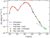 |
Fig. 1 Spectral energy distribution (SED) of CB 26. The red squares and green dots with error bars represent the observational data (Table 1). The dashed black line shows our best-fit model SED. The dashed-dotted blue line represents the adopted contribution from free-free emission. The dotted red line correspondsto the sum flux of dust and free-free emission between 2.9 mm and 4.0 cm. The jump in the SED at ~103 μm is due to the transition from total flux measurements at shorter wavelengths to interferometric data at longer wavelengths, which do not recover the total flux from the extended envelope emission. |
Beam sizes and noise levels of the millimeter maps.
2.2 OVRO
CB 26 was also observed with the Owens Valley Radio Observatory (OVRO) millimeter array between January 2000 and December 2001. Four configurations of the six 10.4 m antennas provided a uv baseline range of 12 – 400 kλ at 1.3 mm (232 GHz). Average single sideband (SSB) system temperatures of the SIS receivers were 300–600 K at 232 GHz. The quasar (QSO) 0355+508, which is located 9° away from CB 26, served as amplitude and phase gain calibrator. The bandpass was calibrated on QSO 3C273. The absolute flux scale was calibrated using the planets Uranus and Neptune. The raw data were exported to the MMA software package (Scoville et al. 1993) for editing and calibration. The MIRIAD software package (Sault et al. 1995) was used for cleaning, mapping and data analysis. The OVRO observations and data are described in more detail in Launhardt & Sargent (2001). For this study, the OVRO data were not used separately, but were combined with the PdBI data to obtain a 1.3 mm map with the best possible uv coverage and signal-to-noise ratio (see below).
2.3 PdBI
In November and December 2005, IRAM3 PdBI observations of CB 26 were carried out using D configuration with five antennas and C configuration with six antennas. The uv baselines of the two array configurations range from 16 to 175 m. The phase center was at αJ2000 = 04h59m50.74s, δJ2000 = 52°04′43.80″. Two receivers were used simultaneously and tuned SSB to around 89 GHz (3.4 mm) and 230 GHz (1.3 mm), respectively. The 3.4 mm data are not used here because of the superior quality of the CARMA 3 mm data. The QSO 0355+508 was used to determine the time-dependent complex antenna gains. The correlator bandpass was calibrated on 3C454.3 and 3C273, and the absolute flux density scale was derived from observations of MWC 349. The flux calibration uncertainty is estimated to be ≲20%. The primary beam size at 1.3 mm was 22″. The SSB system temperature at 230 GHz was in the range 250–450 K. The data were calibrated and imaged using the GILDAS software.
For imaging the continuum emission, we combined the calibrated continuum uv tables from OVRO and PdBI after applying a uv shift of ≈0.2″ to the OVRO data. This was necessary to account for a small source center shift that is likely related to a combination of the unknown proper motion of CB 26 and uncertainties in calibrator coordinates and phase calibration errors. The 1.3 mm data were obtained at the same frequency. Imaging and deconvolution of the continuum data was done with robust uv -weighting (weighting parameter 0), resulting in the synthesized beam sizes and map noise levels listed in Table 2.
2.4 CARMA
The CARMA was a 23-element interferometer located in the Inyo Mountains of California, near Owens Valley. The main CARMA array was used for these observations, consisting of six 10.4-m antennas and nine 6.1-m antennas. CB 26 was observed by CARMA on 2013 November 30 and 2013 December 02 with the antennas in B-configuration, providing a maximum baseline of 900 m and a minimum baseline of ~50 m. At the central frequency of the observations, ~102 GHz (2.9 mm), B-configuration yields an angular resolution of ~0.7″ and a maximum angular scale of ~10″. The correlator was configured in full continuum mode, with 8 GHz of bandwidth subdivided into 16 windows with 500 MHz of bandwidth. The quasar 0136+478 was used for bandpass calibration, 0359+509 was used as the complex gain calibrator, and Mars was used as the absolute flux calibrator.
The data were calibrated and edited using the MIRIAD software package (Sault et al. 1995) using standard methods. The reduced visibility data were then averaged to a single channel and imported into CASA for imaging and self-calibration. The data had sufficient signal to noise for self-calibration to be useful and we performed two rounds of phase-only self-calibration on the data, yielding only a 3% improvement in maximum intensity and a 4% improvement in noise level.
2.5 VLA
Observations of CB 26 were conducted with the VLA in both A and B configuration (program 15A-381). In all observations, data were taken in both Ka-band and C-band. The Ka-band observations were conducted with the correlator in 3-bit mode, sampling a total of 8 GHz of bandwidth that is separated into two 4 GHz basebands. The two basebands were centered at 36.9 GHz and 28.5 GHz (8.1 and 10.3 mm). The C-band observations were conducted with the correlator in 8-bit mode, sampling a total of 2 GHz of bandwidth. This mode was chosen because of the significant radio frequency interference (RFI) in C-band and the 8-bit samplers behaving better in the presence of RFI. Moreover, accounting for the lost bandwidth due to RFI, the 3-bit samplers would not yield significantly greater sensitivity than the 8-bit samplers. The two 1 GHz basebands were centered at 4.7 and 7.3 GHz (4.0 and 6.4 cm). For all observations, 3C84 was observed for bandpass calibration (Ka -band only), the 3C147 was observed for absolute flux calibration and C-band bandpass calibration. The complex gain calibrators for Ka-band and C-band were J0458+5508 and J0541+5312, respectively. Different complex gain calibrators were necessary because J0458+5508 is resolved at C-band, but it was the nearest suitable calibrator for Ka-band.
2.5.1 B-configuration
The B-configuration observations were executed on 2015 February 11 and were conducted in a single ~4.5 h scheduling block. B-configuration provides a maximum baseline of 11 km, resulting in an effective resolution of ~0.2″ at Ka-band and 1″ in C-band. The Ka -band observationswere conducted in fast switching mode to compensate for short-timescale phase variations. The total time of a single on-source scan was 90 s, of which about 20 s was slew time. The time on the calibrator was 42 s, such that one complete cycle, calibrator, source, calibrator, took about 2.9 min. The C-band observations did not require fast switching and each scan on CB 26 was ~600 and ~60 s on the calibrator. The total integration time on CB 26 was ~1.2 h in Ka-band and ~1.15 h in C-band.
2.5.2 A-configuration
Due to scheduling constraints, the A-configuration observations were conducted in three ~1.6 h scheduling blocks on 2015 September 04, September 23, and September 25. A-configuration provides a maximum baseline of 36 km, resulting a resolution of ~0.08″ at Ka-band and ~0.35″ in C-band. The last two executions were taken during the reconfiguration from A to D-configuration (most extended to most compact). However, the antennas on the longest baselines were moved last and there were still 20 antennas in A-configuration on September 23, and 17 antennas on September 25. We followed a similar observing strategy as B-configuration for the fast switching in Ka -band and non-fast switching in C-band; however, we spent 480 s on CB 26 in C-band rather than 600 s as in B-configuration. In each scheduling block, 0.41 h was spent on CB 26 in Ka -band and 0.25 h in C-band. Thus, the total time on source in Ka-band was ~1.25 h and ~0.75 h in C-band.
2.5.3 Data reduction
The raw visibility data were reduced using the scripted VLA pipeline version 1.3.14 in CASA version 4.2.2 (McMullin et al. 2007). However, to obtain better accuracy in the flux calibration, we paused the pipeline at the flux calibration step to flag the flux calibration gain table, ensuring that no bad gain solutions were included in the flux calibration. Following the completed pipeline run, we flagged the gaintables for amplitude and phase and then used them as input to the applycal task using the option mode=flagonly to flag any science data that was associated with the flagged gain solutions. We also then inspected the calibrated science data in a time-averaged amplitude versus frequency plot to look for any obvious signs of bad data that was not excised with the gaintable flagging.
The Ka-band images were produced using the CASA task clean using natural weighting for the combined A and B-configuration imaging. However, we included uv-distances >23 kλ in order to avoid including the antennas that had been moved to their D-configuration positions, which would negatively affect the synthesized beam. In the C-band images, we included uv-distances >10 kλ.
3 Model and modeling
To model the dust continuum data, we used the well-tested radiative transfer code RADMC-3D5 (Dullemond et al. 2012). Our model is composed of a disk and an envelope, similar to the sketch in Fig. 5 of Sauter et al. (2009). Our employed disk model is the same as that in Sauter et al. (2009), yet the envelope model is different from theirs.
3.1 Disk
For the disk we assumed a density profile as described by Shakura & Sunyaev (1973):
![Mathematical equation: \begin{equation*} \begin{aligned} \rho_{\textrm{disk}}(\vec{r}) &\,{=}\,\rho_{\textrm{out,disk}} \left(\frac{r_{\textrm{out}}}{r_{\textrm{cyl}}} \right)^{\alpha} \exp \left(-\frac{1}{2}\left[ \frac{z}{h}\right]^2 \right) \\ &\,{=}\,\frac{\Sigma(\vec{r})}{\sqrt{2\pi}h(r_{\textrm{cyl}})} \exp \left(-\frac{1}{2}\left[ \frac{z}{h}\right]^2 \right),\end{aligned} \end{equation*}](/articles/aa/full_html/2021/02/aa39536-20/aa39536-20-eq5.png) (1)
(1)
where h is vertical scale height as a function of the radial distance rcyl from the z-axis (see also Eq. (3)) z is the cylindrical coordinate, with z = 0 corresponding to the disk midplane. The parameter ρout,disk is determined by the volume density at the outer radius rout, and Σ(r) is the surface density at radius r (see, e.g., Wolf et al. 2003; Stapelfeldt et al. 1998) as
 (2)
(2)
The function h(rcyl) is
 (3)
(3)
where hout is the vertical scale height at the outer radius rout.
The exponents α and k in Eqs. (1) and (3) describe the radial density profile and disk flaring, respectively. Comparison with Eqs. (1)–(3) yields the relation
 (4)
(4)
Considering that the dust destruction radius is at ~0.1 au (Eisner et al. 2005; Mann et al. 2010), the modeling radii of the inner disk were set to 0.1 ≲rin ≲ 100.0 au, while the radii of the outer disk were set to 100.0 ≲rin ≲ 300.0 au (cf. Launhardt et al. 2009; Sauter et al. 2009; Akimkin et al. 2012). This modeling strategy has already been successfully applied to various other edge-on disks, such as the Butterfly-Star IRAS 04302+2247 (Wolf et al. 2003), HK Tau (Stapelfeldt et al. 1998), and HV Tau (Wolf et al. 2003).
3.2 Envelope
For the model of the envelope, we used a spherically symmetric density distribution of the form:
 (5)
(5)
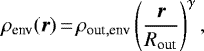
where ρout,env is determined by the dust density at the outer radius Rout of the envelope and γ is the radial density distribution power-law exponent.
To ensure a smooth and realistic density distribution, we did not simply add the two models, but substituted the envelope model (Eq. (5)) with the disk model (Eq. (1)) at ρdisk(r) ≥ ρenv(r). This impliesthat the dust density inside an inner hole in the disk is not zero, but is determined by the density profile of the envelope(cf. Sect. 4.2). Thus, the final model of the density distribution could be described as
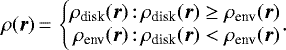 (6)
(6)
We also verified how adding the two density profiles instead of substituting them would affect our results and find that the difference in the total model fluxes is less than 3%, which is smaller than the uncertainties and thus insignificant and negligible. Considering that the dust destruction radius is at ~0.1 au (Eisner et al. 2005; Mann et al. 2010), the modeling radii of the envelope were set as 0.1 ≲r ≲ 900 au. We adopted 1100 au as the radius of the modeled millimeter image space.
3.3 Dust composition
Grain shape
We assume the dust grains to be homogeneous spheres. We limit our model to be simple but also unambiguous by assuming spherical, nonaligned and non-oriented dust grains (Voshchinnikov 2002; Sauter et al. 2009).
Grain composition
For the chemical composition of the dust grains we employ a model that incorporates both silicate and graphite material (see, e.g., “Butterfly star” in Wolf et al. 2003). For the optical data we use the complex refractive indices of smoothed astronomical silicate and graphite (Weingartner & Draine 2001). Since these authors provide refractive indices only for wavelengths shorter than our modeled range, we extrapolate the refractive indices to the wavelength of 6.4 cm. For graphite we adopt the common “ ” approximation. That means, if Qext is the extinction efficiency factor, then
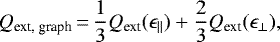 (7)
(7)
where ϵ∥ and ϵ⊥ are the graphite dielectric tensor’s components for the electric field parallel and orthogonal to the crystallographic axis, respectively. As has been shown by Draine & Malhotra (1993), this graphite model is sufficient for extinction curve modeling. For silicate, applying an abundance ratio from silicate to graphite of 3.9 × 10⁻²⁷ cm3 H−1 : 2.3 × 10⁻²⁷ cm3 H−1, we get relative abundances of 62.5% for astronomical silicate and 37.5% graphite ( and
and  ). The grain composition parameters are the same as those in Wolf et al. (2003) and Sauter et al. (2009).
Grain sizes
The grain size distribution is assumed as a power law (Mathis et al. 1977) in the form of
 (8)
(8)
where a is the dust grain radius and n(a) the number of dust grains with a specific radius. We assume an average grain mass density of ρgrain = 3.01 g cm−3. We fix the minimum dust grain size as  (Mathis et al. 1977) in both the disk and envelope. The maximum grain size, amax, is set as a free parameter in the fitting and the choice of amax in Fig. 2 is based on the best-fit model.
3.4 Dust scattering
Light scattering by dust grains can considerably reduce the emission from an optically thick region and lead to an underestimation of the optical depth (Zhu et al. 2019). Scattering also affects the derivation of the maximum grain size of the dust distribution (e.g., Kataoka et al. 2015; Carrasco-González et al. 2019; Liu 2019). Therefore, the effect of scattering in the dust opacity (Natta 1993) is included in our modeling of both the disk and envelope and for the entire wavelength range. Figure 2 shows the average absorption and scattering opacities of the disk and envelope over the whole grain size distribution. The power-law slope p of the grain size distribution is taken to be p = −3.5, with maximum grain sizes of  and
and  , and a minimum grain size of
  .
.
If scattering is ignored, we can no longer fit the IR data points at λ ≲ 20 μm (cf. Fig. 1). The millimeter SED of CB 26 can still be reproduced without scattering, albeit with a slightly different result on the best-fitting value of amax (see Sect. 3.7 and discussion in Sect. 5.3).
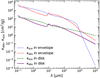 |
Fig. 2 Absorption and scattering coefficients as a function of wavelength for the dust grains in disk and envelope. The power-law slope p of the grain size distribution is taken to be p = −3.5 with |


3.5 Stellar heating
Due to the edge-on orientation of the disk, the central star cannot be observed directly. We thus have to assume the stellar parameters. Observations only hint at a luminosity being L⋆ ≥ 0.5 L⊙ (Stecklum et al. 2004). As a starting point we choose a typical T Tauri star as described by Gullbring et al. (1998). This star has a radius of r⋆ = 2R⊙ and a luminosity of L⋆ = 0.92 L⊙ (cf. Launhardt et al. 2009). Assuming the star to be a black body radiator, this yields an effective surface temperature of T⋆ = 4000 K. We thus set the temperature as a varied parameter around 4000 K in the models. The star will be the only primary source of energy, which means that the disk is passive. The stellar radiation heats the dust, which in turn itself re-emits at longer wavelengths. We neglect accretion or turbulent processes within the models as other possible energy sources.
3.6 Extinction
Extinction has a serious impact on the SED, especially at ultraviolet, optical, and IR wavelengths (e.g., Cardelli et al. 1989; Indebetouw et al. 2005). The interstellar extinction in the wavelength range of 0.85≲λ≲11.6 μm was assumed to follow the relationship described by Cardelli et al. (1989). Therefore, we can use AV as a free parameter in the SED fitting that accounts for both the envelope of CB 26 and interstellar dusty material along the line of sight.
3.7 Fitting
Since the protostellar disk in CB 26 is close to edge-on with an inclination angle of ~88° (Sauter et al. 2009; Launhardt et al. 2009, 2010), the emission is extremely non-spherically symmetric (Jørgensen et al. 2009). Fitting averaged 1D visibility curves could be misleading in such a case. Unfortunately, the extreme edge-on configuration also makes deprojection impossible. Therefore, we only consider the 2D visibilities rather than 1D visibility curves, although the signal-to-noise ratio per visibility point is much lower. We therefore compare the simulations with the observations only in image plane instead of the (u, v)-plane6. We follow three steps to fit the data as outlined below:
We first fit the SED alone, by a manual exploration of the parameter space, to derive a preliminary estimate of the main parameters. The goal is to determine which parameters can be kept fixed (see Table 1), and which parameters need to be varied in our modeling, thus allowing us to significantly reduce the dimensionality of the parameter space to be explored (Pinte et al. 2008). We then systematically explore these remaining free parameters, which cannot be easily extracted from the observations and/or can be correlated with each other. We calculate a rough grid of models and perform a simultaneous fit to all observations. The aim is to find the models that could roughly fit the observations and to narrow down the parameter space. We finally calculate a fine grid of models in the narrowed-down parameter space (in step 2) to fit the observations. This also reduces the uncertainties of the modeled parameters.
In total, more than 300 000 models are performed for fitting. For each comparison between model and observation, we obtain four individual  s; one value for the SED and three values for the millimeter maps at 1.3, 2.9, and 8.1 mm. To measure the fluxes in our model maps for comparison with the SED data, we apply circular apertures with the sizes listed Table 1. We do not consider the 1.1 mm SMA map in the modeling because of the large flux calibration uncertainties (see Sects. 2.1 and 4.1). We also exclude the maps at λ > 8.1 mm from the modeling because they are dominated by free-free emission and have low S/N. To fit 8.1 mm map, we mask the central bright area (≳ 3σ in the 8.1 mm residual map of Fig. 3) because its flux is strongly contaminated by free-free emission (see detailed discussion in Sect. 5.1). To calculate individual
  s, we used the uncertainties listed in Table 1 and in the caption of Fig. 3 at each wavelength for the SED and the millimeter maps, respectively. To avoid fitting into the noise, we define for each of the millimeter maps a polygon that includes the outermost closed 3σ contour, and consider only the flux measurements from inside these polygons. The total
  of one model is then the average over all the individual
  s:
s:
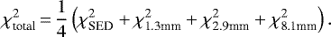 (9)
(9)
Based on the derived  and the best-fit model
  , the modeling uncertainties (minimum and maximum) are estimated by altering each free parameter value alone for the set of models that fulfill the
  criterion (see a similar criterion in Robitaille et al. 2007). Although the choice of this level is somewhat arbitrary, it provides a range of acceptable fits to the eye, and reflects a dependence on each free parameter. All the input modeling parameter space and the output best-fit parameters are listed in Table 3.
Overview of parameter ranges used in the modeling.
4 Results
4.1 Comparison between observation and simulation
The total  for the best-fit model to the SED and the three millimeter maps at 1.3, 2.9, and 8.1 mm is
  (Table 4). Figure 1 shows the SED between 0.9 μm and 6.4 cm together with this best-fit model SED, which fits the observations quite well with
  . The sudden flux decrease at λ ~ 1 mm in the SED (Fig. 1) is related to the inability of the interferometric observations at longer wavelengths to recover the total flux from the extended envelope. The fluxes at these wavelengths are therefore measured in smaller apertures (Table 1) that contain only the disk emission, as opposed to the total disk+envelope flux measured at the shorter wavelengths.
Figure 3 shows the observed and modeled intensity maps at 1.3, 2.9, and 8.1 mm. The maps of the best-fit model at 1.3, 2.9, and 8.1 mm have  ,
,  , and
, and  , respectively. The residual map at 1.3 mm shows some non-axisymmetric ± 3σ contours, which are probably phase noise or deconvolution artifacts. Figure 4 displays the intensity distribution cuts along the major and minor axes in the observed and simulated maps at 1.3, 2.9, and 8.1 mm (see Fig. 3). The discrepancies at all three wavelengths (at 8.1 mm considering only regions outside the masked central free-free peak) are smaller than 3σ.
If the 1.1 mm is included for calculating the best-fit model, the total  will be
  7, which is almost twice as high as when excluding it. The individual χ2 values listedin Table 4 indicate that the fits to both the 1.1 mm and the 1.3 mm are particularly bad, with
  and
and 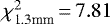 , when the 1.1 mm map is included. This means, these two maps cannot be fit well together, for example, they disagree. We suspect the main reason for this discrepancy to be the poor flux calibration of the 1.1 mm SMA data (see Sects. 2.1 and 3.7). The observed and modeled intensity maps for the fit including the 1.1 mm map are shown in appendix Fig. A.1 (corresponding to Fig. 3), and their intensity distribution cuts along the major and minor axes are presented in appendix Fig. A.2 (corresponding to Fig. 4). Nevertheless, the best-fit parameter values listed in Table A.1 all agree within the uncertainties with the results obtained without the 1.1 mm map and the constraints on the maximum grain size in the disk are completely unaltered. Therefore, we adopt the best-fit model obtained without the 1.1 mm map for further discussion8.
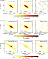 |
Fig. 3 Observed and modeled intensity maps at 1.3, 2.9, and 8.1 mm. The modeled maps have smaller pixel sizes than the observed maps, but are convolved to the same beam sizes as the respective observations (shown as ellipses in the lower left corners). The contour levels in each residual image start at −3σ, 3σ in steps of 3σ with σ1.3mm = 0.019 mJy pixel−1 (1 pixel = 0.1″ × 0.1″ at 1.3 mm), σ2.9mm = 1.37 μJy pixel−1 (1 pixel = 0.05″ × 0.05″ at 2.9 mm), and σ8.1mm = 0.038 μJy pixel−1 (1 pixel = 0.01″ × 0.01″ at 8.1 mm) in the observations. Solid green and dotted blue lines show the directions of major and minor axes in the observation and simulation panels (cf. Fig. A.2). The central compact emission within the red-dashed ellipse at 8.1mm residual map was masked for fitting (see details in Sect. 3.7). |
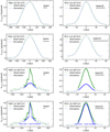 |
Fig. 4 Intensity distribution cuts along the major and minor axes (see Fig. 3) in observations and simulations at 1.3, 2.9, and 8.1 mm. The pixel size at each wavelength is listed in the caption of Fig. 3. The central peak at 8.1 mm was masked for fitting (marked with thick line, see details in Sect. 3.7 and Fig. 3). Lowest panel: 8.1 mm free-free emission is included by assuming a point source with flux ~77 μJy (see Sect. 5.1). |
χ2 distributions for the best-fit model.
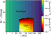 |
Fig. 5 Density structure as a function of radius r and polar angle θ in spherical coordinates (90° is the equatorial plane with z = 0). The disk and envelope locations are indicated by different color scales. The contours with numbers indicate different optical depths at 1.3 mm. |
4.2 Density
Figure 5 displays the density structure as a function of radius r and polar angle θ in spherical coordinates (90° is the equatorial plane with z = 0). It clearly shows the density structures in the disk (see Eq. (1)) and envelope (see Eq. (5)). The disk has an inner hole like already found before (Launhardt et al. 2009; Sauter et al. 2009; Akimkin et al. 2012). Although our best-fit hole radius of 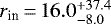 au is somewhat smaller than derived before, all four hole size estimates agree within the uncertainties. The maximum dust density in the disk is ρmax ≈ 3.5 × 10⁻¹⁵ g cm−3, located at the inner edge of the disk with rin = 16.0 au. We also overlay the distribution of optical depths at 1.3 mm on the density map. The regions close to midplane with 90° − θ≲10° have moderate optical depth with τ1.3mm≳1.0.
4.3 Temperature
Figure 6 displays the temperature structure as a function of radius r and polar angle θ in spherical coordinates. Figure 7 shows the radial temperature distribution along the midplane of the disk and envelope. The envelope temperature profile generally follows a power-law, both inside the inner hole of the disk and outside the disk. Snow-lines of volatile species play an important role in planet formation theories (e.g., Pontoppidan et al. 2014). Assuming a water ice sublimation temperature range of 150−170 K (e.g., Podolak & Zucker 2004; Liu et al. 2017), the water snowline in the disk midplane is located at a radius range of ~4.1–5.4 au, much smaller than the inner radius (rin = 16 au) of the disk (see Figs. 6 and 7). The temperature in the disk is 20≲Tdisk≲90 K, which is much lower than the water ice sublimation temperature. Close to the outer edge of the disk, where, by chance, the CO snow line (~20 K) is located, the radial temperature profile turns flat and gradually becomes steeper when going further inward in the disk. CO freezes out at about 20 K and the disk as a whole does not get below 20 K. This is further evidence that CB 26 is still a very young embedded disk, which tends to be warmer than more evolved protoplanetary disks (Burke & Brown 2010; van ’t Hoff et al. 2018a,b).
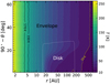 |
Fig. 6 Temperature structure as a function of radius r and polar angle θ in spherical coordinates. The possible CO snow line at ~20 K and the water ice sublimation temperature range of 150–170 K are indicated with three horizontal lines. |
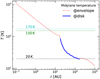 |
Fig. 7 Temperature distribution along the disk and envelope midplane. The possible CO snow line of 20 K and ice sublimation temperature range of 150–170 K are indicated with three dashed lines. |
4.4 Mass
Our best-fitmodel suggests dust masses in the disk and envelope of  M⊙ and
  M⊙, respectively. Assuming a constant gas-to-dust mass ratio of 100 (Glauser et al. 2008), their gas masses are
  M⊙ and
  M⊙, respectively. Uncertainties are difficult to quantify because they largely depend on the absolute value of the dust absorption coefficient and on the unconstrained gas-to-dust mass ratio. Furthermore, the total extent of the envelope is also poorly constrained and the choice of our cut-off radius at 900 au (Sect. 3.2) is arbitrary. Based on single-dish millimeter and Herschel far-infrared (FIR) data, Launhardt et al. (2013) derive an envelope radius and total mass of 1 × 10⁴ au and ≈0.22 M⊙9, respectively. The mass of the disk thus amounts to about 14% of the central star mass (M⋆ = 0.55M⊙; Launhardt et al., in prep.), which is consistent with hydrodynamic simulations of marginally self-gravitating disks (Nelson et al. 2000). Thus, the CB 26 disk stands out as one of the most extended and massive Class I disks (e.g., Tobin et al. 2020; Tychoniec et al. 2020). Hogerheijde (2001) showed that rotationally supported disks grow as long as they are still embedded and accrete from the envelope, and start decreasing in size when the envelope is dispersed. This implies that such disks reach their maximum size at the transition from the fully embedded to the T Tauri phase. With CB 26 we have caught a disk just at this transition stage when it reaches the maximum disk size.
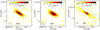 |
Fig. 8 Modelled optical depth contours (τ1.3mm, τ2.9mm, τ8.1mm), overlaid on the observed intensity maps at 1.3, 2.9, and 8.1 mm, respectively. The observed intensity maps are identical to those shown in the leftmost panels of Fig. 3, and show the dust emission convolved with the indicated beam sizes, while the optical depth contours are not convolved. The optical depth value is indicated at each corresponding contour. The zoomed-in optical depth distributions are displayed in Fig. 9. |
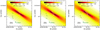 |
Fig. 9 Zoomed-in modeled optical depth contours at 1.3, 2.9, and 8.1 mm, overlaid on the (also unconvolved) colour map of the millimeter opacity slope, βmm, derived from the best-fit model maps (cf. Figs. 3 and 11). The optical depth values are indicated at each corresponding contour. The pixel size for all three maps is 0.016″ × 0.016″. |
4.5 Optical depth
Figure 8 displays the modeled optical depth contours of the dust emission overlaid on the observed intensity maps at 1.3, 2.9, and 8.1 mm. Figure 9 shows the zoomed-in optical depth distributions, overlaid on Fig. 10 shows the optical depth distributions at 1.3, 2.9, and 8.1 mm along the major radial direction. These optical depth distributions and profiles demonstrate that the dust emission along the disk midplane is only moderately optically thick in the innermost parts of the disk (r1.3mm≲65 au, r2.9mm≲50 au, and r8.1mm≲30 au), while most parts of the outer disk are optically thin at all three wavelengths.
4.6 Grain size distribution
For both the envelope and the disk we adopted a power-law grain size distribution with exponent −3.5 (Eq. (7)), a minimum grain size of amin = 10 nm, and let the maximum grain size vary in the modeling (Sect. 3.3). As indicated in Table 3, we derive a best-fit maximum grain size for the envelope emission of  mm, which is already significantly larger than upper grain sizes if ISM dust given in the literature. Our best-fit models for the maximum grain size in the disk indicate
  cm. Hence, the dust emission from the disk is incompatible with both ISM-type dust and the grain size distribution in the envelope, but requires the existence of already pebble-sized bodies with diameters of about 10 cm. In Sect. 5.3, we discuss the robustness and implication of this finding.
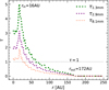 |
Fig. 10 Modelled dust optical depth distribution along the major radial direction at 1.3, 2.9, and 8.1 mm in Fig. 9. |
5 Analysis and discussion
5.1 Free-free emission at 8.1 mm
The physics behind the ionization around high-mass stars is reasonably well understood as arising from photoionization due to the strong UV flux from such objects. Ionization around low-mass stars is much less understood. A few mechanisms have been proposed for low-mass stars to produce the ionization responsible for the detected free-free emission (Anglada et al. 1998; Scaife 2012). The centimeter-wavelength emission of young stars is often dominated by hot plasma in the system, either gyrosynchrotron emission associated with chromospheric activity or thermal bremsstrahlung emission from partially ionized winds (Wilner et al. 2005).
In CB 26, the sharp central peak in the 8.1 mm map cannot be fitted with only dust emission in the simulation. Instead, the observed intensity distribution requires the contribution from a compact nonthermal source in addition to the thermal dust emission from the disk (see Figs. 3 and 4). Assuming that this compact nonthermal source is free-free emission and that the fluxes at 4 and 6.4 cm are dominated by this free-free emission, the estimated spectral index for the non-dust emission would be ≈0.13. This indicates that the ionized wind from star is quite inhomogeneous (Condon & Ransom 2016). One can also extrapolate that the free-free contribution at 8.1 mm is ≈77 μJy, which accounts for ≈7% of the observed total 8.1 mm flux (see bottom panel of Fig. 4). The residual of the sharp peak between observation and simulated dust emission amounts to about ≈110 μJy or 10% of the observed total flux at 8.1 mm. Hence, the total flux of the sharp central peak at 8.1 mm is comparable to the extrapolated free-free contribution at this wavelength. We can therefore safely assume that the sharp peak is mainly produced by free-free emission, while the wide wings in the 8.1 mm map are produced by dust emission.
Since CB 26 is driving a collimated bipolar outflow (Launhardt et al. 2009), a jet-origin (shock ionization) of this free-free emission is the most likely scenario. An alternative explanation could be that the central peak at 8.1 mm is tracing a photoevaporating region in the circumstellar disk (Pascucci et al. 2012; Rodríguez et al. 2014). This photoevaporation region must be much smaller than the observed dust disk and could well occupy and cause the inner whole that is observed at millimeter wavelengths (Sect. 5.2).
While we can explain the central peak in the 8.1 mm emission map (Fig. 4) with compact free-free emission (Sect. 5.1), there is still significant extended residual emission at r ≈ 50−65 au when only the best-fit dust emission model of the disk and an unresolved free-free emission region are taken into account (Figs. 3 and 4). We discuss this residual excess emission in Sect. 5.3.
5.2 The inner hole
The observed 1.3 mm intensity distribution along the major axis of the disk, shown in Fig. 4, exhibits a suspicious plateau at the center, similar but less prominent than that in the OVRO-only map used by Sauter et al. (2009). This plateau is less prominent or not visible at all in the 1.1, 2.9, and 8.1 mm maps. At 1.1 and 2.9 mm, this may be related to the lower angular resolution of these maps (Table 2). The 8.1 mm map has a higher angular resolution, but the compact free-free emission (Sect. 5.1) may mask a possible plateau or dip. The plateau in the 1.3 mm map may be caused by an inner hole in the disk or could be the result of the (moderate) optical thickness of the millimeter dust emission from the innermost parts of the disk (Fig. 10), such that enough flux from the (warmer) inner disk is obscured.
In our modeling, pure optical depth effects in a disk without inner hole could clearly not reproduce the observed dust emission profiles. Instead, an inner whole was needed. In our model, this inner whole is not completely dust-free, but is still filled with the dust from the envelope model (Sect. 3.2). The size of this inner hole is poorly constrained by our models. We derive a best-fit radius of  au (Table 3). The observed plateau at 1.3 mm could be reproduced in the simulations only if we force the size of the inner hole to be rin≳30 au, which is still within the range of uncertainties given above. In this case, the plateau would still not be visible at 1.1 and 2.9 mm (due to the large beam size), like in the observed maps.
5.3 Grain growth
Our best-fit radiative transfer model, which has amax of the grains size distribution as a free parameter (Table 3), and the uncertainty ranges indicate that the dust grains in the disk have already grown to pebbles with diameters of the order 10 cm ( cm, Table 3). Even the dust in the envelope contains at least submillimeter-sized grains (
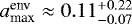 mm), which is several orders of magnitude larger than the upper end of the grain size distribution in the ISM (e.g., Weingartner & Draine 2001). If we use maximum grain sizes
  in the disk and
  in the envelope, as in Sauter et al. (2009), we cannot reproduce the SED, even after testing a large parameter space. The reason for this discrepancy with Sauter et al. (2009) is most likely manifold. Besides a slightly different treatment of the envelope, we could in our new study include the Herschel FIR measurements and, more importantly, the new 8.1 mm VLA data, which provide much more robust constraints on the millimeter dust emissivity than the 1.3 and 3 mm data only. As we show in Appendix A and discuss in Sect. 4.1, our result is not affected by in- or excluding the 1.1 mm SMA map, and can thus be considered robust.
The best-fit modeled optical depth distributions, displayed in Fig. 10 (see also Sect. 4.5), shows that the thermal emission at all millimeter wavelengths is optically thin (τ < 1) in the outer disk (r ≳ 60 au), and becomes only moderately optically thick (τ1.3mm < 5.0, τ2.9mm < 3.1, τ8.1mm < 1.9) in the innermost parts of the disk at r ≲ 50 au, and even there only close to the disk midplane (Figs. 8 and 9). Thus, we can exclude that a not optimally modeled optical depth distribution could have significantly affected our results. As explained in Sect. 3.4, we have also taken into account scattering in our modeling (Fig. 2), such that the two main simplifications that could lead to an overestimation of amax are avoided here (e.g., Carrasco-González et al. 2019).
Even if we ignore scattering (Sect. 3.4), we can still reproduce the millimeter SED and maps of CB 26 with an only slightly differing best-fit value of amax. The reason why scattering makes a much smaller difference for CB 26 as compared to, for example, the ALMA-based study of HL Tau presented recently by Carrasco-González et al. (2019), is manifold. First, the peak optical depth in our CB 26 data is much smaller than in the ALMA data of HL Tau. This is related to both the higher angular resolution of the ALMA data as compared to our data (both sources are located at approximately the same distance), and to the fact that CB 26 is seen edge-on, while HL Tau is seen nearly pole-on. Due to both the different beam sizes and the different projections, small-scale structures with locally increased optical depths are much better resolved in HL Tau than in CB 26. This in turn could imply that possible substructures (rings, spirals, clumps) with increased optical depths and a potentially differing grain size distribution might be hidden since they are unresolved and not modeled in our CB 26 data (our disk model does not include small-scale substructures since there are no such observational constraints, see Sect. 3.1). On the other hand, such hypothesized over-dense small-scale substructures in the CB 26 disk would occupy only a tiny areal fraction and contribute only very little to the observed emission since they are expected to be confined to the disk midplane, which is seen edge-on. Hence, even if present, such small-scale structures would not significantly affect our results for the bulk of the dust in the CB 26 disk.
In our model, grain sizes are well-mixed throughout the disk and possible vertical settling of the largest grains has not been taken into account. To verify if ignoring vertical dust settling could have affected our conclusions on grain growth in the CB 26 disk, we also perform a test in which the vertical scale height (h; see also Eq. (3)) is a function of the grain size, a:
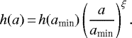 (10)
(10)
Here, h(amin) is the scale height for the smallest dust grains, while the parameter ξ quantifies the degree of dust settling. We fix ξ = –0.1, which is typically found for other systems, for instance the IM Lup disk (Pinte et al. 2008). We find that the millimeter fluxes of the settled disk are overall slightly lower than those of the well-mixed model. This is due to the fact that large dust grains are concentrated close to the midplane where the temperature is low. To compensate the flux deficit, a higher total dust mass in the disk is required to fit the observation, which in turn results in a slightly larger optical depth. Nevertheless, as long as large dust grains are only moderately depleted, but still present at larger scale heights, the slope of the millimeter SED remains nearly unchanged. Therefore, we conclude that dust settling does not have a significant impact on the derived maximum grain size.
However, as we show in Sect. 5.1 and Figs. 3 and 4, our best-fit model with amax = 5 cm throughout the disk anda compact (unresolved) central region with free-free emission still leaves significant extended 8.1 mm residual emission at r ≈ 50−65 au. Since the 8.1mm thermal dust emission at these radii is clearly optically thin (Fig. 10), and the moderate optical thickness of the emission at shorter wavelengths has been taken into account in our modeling, this residual emission could hint at a radial change in the dust grain size distribution, for example, the presence of even larger grains in the inner ≈65 au of the disk. Because of the uncertainties involved at this level of detail and the missing observational constraints on size scales <50 au (the projected beam size at 8.1 mm is ≈18 au, while it is only ≈52 au at 1.3 mm; see Table 2), we do not involve a model with a step function or radial gradient in amax(r), and thus do not attempt to quantify this possible further grain growth in the inner disk.
Since the dust emission is optically thin throughout most of the disk, a large value of amax, for example, the presence of dust grains that are significantly larger than the observing wavelength, should become directly evident in the spectral index of the millimeter dust emission, αmm, which relates for optically thin emission to the spectral index of the dust absorption coefficient as βmm = αmm − αP, where αP = dlgB(ν, T)∕dlgν is the spectral slope of the Planck function. With a dust temperature T ≈20…100 K in disk (Fig. 6), the spectral index will be αp = 1.80…1.96 between 1.3 and 2.9 mm. Considering that the majority of the disk (Fig. 7) has a dust temperature of around 40 K, we could reasonably adopt αP = 1.9 throughout the disk, thus we assume βmm = αmm − 1.9 in this work. Indeed, we derive a millimeter spectral index of the observed integrated fluxes at 1.3 and 2.9 mm of α1.3~2.9mm = 2.63 ± 0.40, which for optically thin emission corresponds to a mean absorption opacity slope of β1.3~2.9mm = 0.73 ± 0.40. For the corresponding 1.3 to 8.1 mm slope we obtain α1.3~8.1mm = 2.56 ± 0.30, which is consistent with α1.3~2.9mm.
Furthermore, Fig. 11 shows the spatially resolved millimeter opacity slope profiles, derived under the optically thin assumption from the spectral index slopes, along the major axis of the disk in the observations and the best-fit model. Both are convolved at all wavelengths to the beam size of the 2.9 mm map (Table 2). Comparing the observations directly, we derive 0.36 ≲ β1.3−2.9mm ≲ 1.24 with a relatively strong positive radial gradient (Fig. 11). Comparison of the 1.3 mm map with the longer wavelength map at 8.1 mm results in an approximately radially constant slope of β1.3~8.1mm ≈ 0.73 ± 0.05. Since already a slight mismatch in the effective beam sizes or a slight pointing offset between the maps at different wavelength can result in such a radial gradient, we do not try to interpret these gradients here, but look at the simulated best-fit maps instead, which do not have these problems.
Comparing the convolved simulated best-fit maps, we derive 0.62 ≲ β1.3-2.9mm ≲ 0.82 and 0.67 ≲ β1.3-8.1mm ≲ 0.92, with a slight positive radial gradient in both cases (Fig. 11). This positive radial gradient is expected and is mainly caused by the relative contribution from the envelope (with smaller dust grains and larger βmm), which increases with increasing impact parameter. Also contributing, but to a lesser degree, is the non-negligible optical depth, which increases toward smaller impact parameters (Fig. 10), and the radial temperature gradient (Fig. 6). Altogether, the spectral slope of the integrated fluxes, as well as the spatially resolved radial profiles of the spectral slopes derived from both the observed and the best-fit modeled maps all consistently suggest a mean millimeter absorption opacity slope of βmm ≈ 0.7 ± 0.4 for the outer disk (r ≳ 50 au) of CB 26.
Such a small value of βmm < 1 is understood to indicate that the dust particles have grown into large grains of at least millimeter size or even larger (e.g., Testi et al. 2003; Rodmann et al. 2006; Pinte et al. 2008; Tobin et al. 2013; Tazzari et al. 2016). We want to stress here that the millimeter spectral slope in CB 26 can only be related so directly to the maximum grain size because our models have shown that the emission is optically thin. Ricci et al. (2010a) derive a similar value for the mean absorption opacity slope in ρ-Ophiuchi protoplanetary disks, in which the grains are also thought to have grown to millimeter or centimeter sizes.
The presence of centimeter-sized dust grains in the about 1 Myr old CB 26 disk is consistent with models of grain growth and radial drift in protoplanetary disks by, for example, Birnstiel et al. (2010). Moreover, our finding indicates that solids grow rapidly already during the first million years in a protostellar disk, making it thus possible that the Class II (transitional) disks are already seeded with large particles, making it much more likely that they already contain large bodies and perhaps even planetesimals (e.g., Johansen et al. 2014). Furthermore, the dust masses of Class II disks inferred from millimeter surveys (e.g., Andrews et al. 2013; Ansdell et al. 2016; Pascucci et al. 2016) could partially reflect this growth of solids to large sizes that are no longer emitting efficiently.
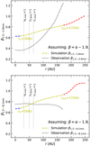 |
Fig. 11 Millimeter absorption opacity slopes βmm along the major axis of the disk in the observations and the best-fit model. The slopes β1.3-2.9mm and β1.3-8.1mm are derived from spectral indexes α1.3-2.9mm between 1.3 and 2.9 mm, and α1.3-8.1mm between 1.3 and 8.1 mm, respectively (see text). All data have been convolved to the angular resolution of the CARMA 2.9 mm map (Table 2). The contribution from free-free emission at 8.1 mm has been removed (see Sect. 3.7 and Fig. 4). |
5.4 Toomre stability
The gravitational stability of the disk can be tested using the Toomre criterion (Toomre 1964), which describes when a disk becomes unstable to gravitational collapse. The Toomre Q parameter is defined as
 (11)
(11)
where  is the local sound speed,
  is the angular velocity for Keplerian rotation (Knigge 1999), and Σgas stands for the surface density of the gas in the disk, which can be derived from the surface density of the dust assuming a constant gas-to-dust mass ratio of 100 throughout the disk for simplicity (Glauser et al. 2008). The corresponding parameters are listed in Table 3. In terms of Q, a disk is unstable to its own self-gravity if Q < 1, and stable if Q > 1. Figure 12 displays the Toomre Q parameter as a function of radius in the CB 26 disk. It clearly shows that Q is greater than unity for the entire disk (1.8≲Q≲16.4), indicating that the disk is gravitationally stable. However, in contrast to the inner disk, the outer parts of the disk at r≳80 au have Q values close to unity (1.8≲Q≲3.5), suggesting it is approaching marginal instability. In numerical simulations of rapid accretion, Kratter et al. (2010) found that a marginally unstable outer disk will not fragment, but may generate spiral arms (see also, e.g., Rice et al. 2003; Stamatellos & Whitworth 2008; Dong et al. 2018). Unfortunately, this cannot be verified directly observationally in CB 26 due to the extreme edge-on orientation.
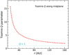 |
Fig. 12 Toomre Q parameter as a function of radius r along the disk midplane. Q = 1 is indicated with a dotted line. |
6 Summary and conclusions
The Bok globule CB 26 harbors a young (≈1 Myr) low-mass (≈0.55 M⊙) star that is surrounded by a massive circumstellar disk seen nearly edge-on, which is in turn still embedded in a thin remnant envelope. Combining the well-sampled SED between 0.9 μm and 6.4 cm, high-angular-resolution millimeter continuum observations at 1.1, 1.3, 2.9, and 8.1 mm, and using the radiative transfer code RADMC-3D (Dullemond et al. 2012), we conduct a detailed modeling of the dust emission from the CB 26 circumstellar disk. The models are fitted simultaneously to the complete SED and to the image plane data of the interferometric dust continuum emission maps at 1.3, 2.9, and 8.1 mm.
From the best-fit models to the thermal dust emission, we infer an outer radius of the disk of rout = 172 ± 22 au, and a size of the inner hole of  au. Assuming a constant gas-to-dust mass ratio of 100, we derive a total gas mass in the disk of Mdisk = 7.6 × 10⁻² M⊙. The mass of the disk amounts to ≈14% of the mass of the central star. The mass of the surrounding envelope remains largely unconstrained since our model takes into account only the innermost 900 au (3.3 × 10⁻² M⊙ < Menv ≲ 0.22M⊙). The other best-fit model parameters are listed in Table 3. Thus the disk around CB 26 stands out as one of the most extended and massive Class I disks.
We find that the central part of the disk contains an unresolved compact region of free-free emission, which significantly contributes to the 8.1 mm flux and completely dominates the cm emission. We cannot constrain whether this free-free emission is related to a jet (shock ionization) or originates from a photoevaporation region in the inner hole of the disk. For our modeling of the thermal dust emission, we treat this free-free emission region as point-like, extrapolate its contribution to the 8.1 mm emission from the spectral slope of the 4.0 and 6.4 cm fluxes, subtract it from the 8.1 mm map, and exclude the contaminated central region in the 8.1 mm map from the model fitting.
We find that the thermal dust emission from the outer disk (r ≳ 60 au) is optically thin (τ ≪ 1) at all millimeter wavelengths, while the emission from the midplane of the inner disk (r ≲ 50 au) becomes moderately optically thick (τ1.3mm < 5.0, τ2.9mm < 3.1, τ8.1mm < 1.9). Our best-fit radiative transfer models, which assume a grain size distribution with power-law exponent − 3.5 and amin = 5 nm, indicate that the dust grains in the disk have already grown to pebbles with diameters of the order 10 cm. Even the dust in the envelope contains already at least submm-sized grains, for example, much larger than what is considered the upper end of the grain size distribution in the ISM.
Our best-fit model still leaves significant extended 8.1 mm residual emission at r ≈ 50−65 au, which we interpret as a radial change in the grain size distribution and the presence of even larger particles in the inner disk. However, we are not able to reliably quantify their size.
Since our detailed models show that the millimeter dust emission from the outer disk is completely optically thin, and the contribution from moderately optically thick emission from the midplane in the inner disk is very small, we can directly relate the spectral slope of the millimeter dust emission, αmm, to the spectral index of the dust absorption coefficient, βmm, and to the size of the largest dust grains, amax, when these are of the same order or larger than the observing wavelength. Indeed, we derive a mean millimeter absorption opacity slope of βmm ≈ 0.7 ± 0.4 for the entire outer disk of CB 26, which is consistent with the presence of millimeter- to centimeter-sized dust particles.
Altogether, our robust finding of the presence of at least centimeter-sized bodies in the CB 26 disk indicates that solids grow rapidly already during the first million years in a protostellar disk, making it thus possible that the slightly more evolved Class II (transitional) disks are already seeded with large particles. This in turn makes it likely that these disks may already contain larger bodies and perhaps even planetesimals.
Last but not least, we find the inner disk of CB 26 (r ≲ 80 au) is gravitationally stable, while the outer disk may be approaching marginal instability and thus be prone to generating spiral arms. Unfortunately, this cannot be verified observationally due to the extreme edge-on orientation of CB 26.
Acknowledgements
We thank the anonymous referee for constructive comments that improved our study. This work is supported by the National Natural Science Foundation of China Nos. 11703040, 11743007, 11503087, 11973090, and the Natural Science Foundation of Jiangsu Province of China No. BK20181513. C.-P.Z. acknowledges supports from the MPG-CAS Joint Doctoral Promotion Program (DPP), the China Scholarship Council (CSC) in Germany as a postdoctoral researcher, the NAOC Nebula Talents Program, and the Cultivation Project for FAST Scientific Payoff and Research Achievement of CAMS-CAS. T.H. acknowledges support from the European Research Council under the Horizon 2020 Framework Program via the ERC Advanced Grant Origins 83 24 28.
Appendix A Results with 1.1 mm map included
Parameters in the best-fit model with 1.1 mm map included.
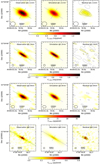 |
Fig. A.1 Observed and modeled intensity maps at 1.1, 1.3, 2.9, and 8.1 mm. The modeled maps have smaller pixel sizes than the observed maps, but are convolved to the same beam sizes as the respective observations (shown as ellipses in the lower left corners). The contour levels in each residual image start at −3σ, 3σ in steps of 3σ with σ1.1mm = 0.028 mJy pixel−1 (1 pixel = 0.1″ × 0.1″ at 1.1 mm), σ1.3mm = 0.019 mJy pixel−1 (1 pixel = 0.1″ × 0.1″ at 1.3 mm), σ2.9mm = 1.37 μJy pixel−1 (1 pixel = 0.05″ × 0.05″ at 2.9 mm), and σ8.1mm = 0.038 μJy pixel−1 (1 pixel = 0.01″ × 0.01″ at 8.1 mm) in the observations. Solid green and dotted blue lines show the directions of major and minor axes in the observation and simulation panels (cf. Fig. A.2). The central compact emission within the red-dashed ellipse at 8.1mm residual map was masked for fitting (see details in Sect. 3.7). |
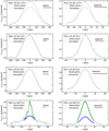 |
Fig. A.2 Intensity distribution cuts along the major and minor axes (see Fig. A.1) in observations and simulations at 1.1, 1.3, 2.9, and 8.1 mm. The pixel size at each wavelength is listed in caption of Fig. A.1. The central peak (marked with thick line) at 8.1 mm was masked for fitting (see details in Sect. 3.7 and Fig. A.1). |
References
- Akimkin, V. V., Pavlyuchenkov, Y. N., Launhardt, R., & Bourke, T. 2012, Astron. Rep., 56, 915 [NASA ADS] [CrossRef] [Google Scholar]
- Andrews, S. M., Rosenfeld, K. A., Kraus, A. L., & Wilner, D. J. 2013, ApJ, 771, 129 [NASA ADS] [CrossRef] [Google Scholar]
- Anglada, G., Villuendas, E., Estalella, R., et al. 1998, AJ, 116, 2953 [NASA ADS] [CrossRef] [Google Scholar]
- Ansdell, M., Williams, J. P., van der Marel, N., et al. 2016, ApJ, 828, 46 [Google Scholar]
- Bayo, A., Olofsson, J., Matrà, L., et al. 2019, MNRAS, 486, 5552 [CrossRef] [Google Scholar]
- Birnstiel, T., Dullemond, C. P., & Brauer, F. 2010, A&A, 513, A79 [NASA ADS] [CrossRef] [EDP Sciences] [Google Scholar]
- Burke, D. J., & Brown, W. A. 2010, Phys. Chem. Chem. Phys., 12, 5947 [NASA ADS] [CrossRef] [PubMed] [Google Scholar]
- Cardelli, J. A., Clayton, G. C., & Mathis, J. S. 1989, ApJ, 345, 245 [NASA ADS] [CrossRef] [Google Scholar]
- Carrasco-González, C., Sierra, A., Flock, M., et al. 2019, ApJ, 883, 71 [NASA ADS] [CrossRef] [Google Scholar]
- Condon, J. J., & Ransom, S. M. 2016, Essential Radio Astronomy (Princeton: Princeton University Press) [Google Scholar]
- Dong, R., Najita, J. R., & Brittain, S. 2018, ApJ, 862, 103 [NASA ADS] [CrossRef] [Google Scholar]
- Draine, B. T., & Malhotra, S. 1993, ApJ, 414, 632 [NASA ADS] [CrossRef] [Google Scholar]
- Dullemond, C. P., Juhasz, A., Pohl, A., et al. 2012, Astrophysics Source Code Library [record ascl:1202.015] [Google Scholar]
- Eisner, J. A., Hillenbrand, L. A., White, R. J., Akeson, R. L., & Sargent, A. I. 2005, ApJ, 623, 952 [NASA ADS] [CrossRef] [Google Scholar]
- Espaillat, C., Muzerolle, J., Najita, J., et al. 2014, Protostars and Planets VI, eds. H. Beuther, R. S. Klessen, C. P. Dullemond, & T. Henning (Tucson, AZ: University of Arizona Press), 497 [Google Scholar]
- Glauser, A. M., Ménard, F., Pinte, C., et al. 2008, A&A, 485, 531 [NASA ADS] [CrossRef] [EDP Sciences] [Google Scholar]
- Gullbring, E., Hartmann, L., Briceño, C., & Calvet, N. 1998, ApJ, 492, 323 [NASA ADS] [CrossRef] [Google Scholar]
- Henning, T., Wolf, S., Launhardt, R., & Waters, R. 2001, ApJ, 561, 871 [NASA ADS] [CrossRef] [Google Scholar]
- Ho, P. T. P., Moran, J. M., & Lo, K. Y. 2004, ApJ, 616, L1 [NASA ADS] [CrossRef] [Google Scholar]
- Hogerheijde, M. R. 2001, ApJ, 553, 618 [NASA ADS] [CrossRef] [Google Scholar]
- Indebetouw, R., Mathis, J. S., Babler, B. L., et al. 2005, ApJ, 619, 931 [NASA ADS] [CrossRef] [Google Scholar]
- Johansen, A., Blum, J., Tanaka, H., et al. 2014, Protostars and Planets VI, eds. H. Beuther, R. S. Klessen, C. P. Dullemond, & T. Henning (Tucson, AZ: University of Arizona Press), 547 [Google Scholar]
- Jørgensen, J. K., van Dishoeck, E. F., Visser, R., et al. 2009, A&A, 507, 861 [NASA ADS] [CrossRef] [EDP Sciences] [Google Scholar]
- Kataoka, A., Muto, T., Momose, M., et al. 2015, ApJ, 809, 78 [NASA ADS] [CrossRef] [Google Scholar]
- Knigge, C. 1999, MNRAS, 309, 409 [NASA ADS] [CrossRef] [Google Scholar]
- Kratter, K. M., Matzner, C. D., Krumholz, M. R., & Klein, R. I. 2010, ApJ, 708, 1585 [NASA ADS] [CrossRef] [Google Scholar]
- Launhardt, R., & Henning, T. 1997, A&A, 326, 329 [Google Scholar]
- Launhardt, R., & Sargent, A. I. 2001, ApJ, 562, L173 [NASA ADS] [CrossRef] [Google Scholar]
- Launhardt, R., Pavlyuchenkov, Y., Gueth, F., et al. 2009, A&A, 494, 147 [NASA ADS] [CrossRef] [EDP Sciences] [Google Scholar]
- Launhardt, R., Nutter, D., Ward-Thompson, D., et al. 2010, ApJS, 188, 139 [NASA ADS] [CrossRef] [Google Scholar]
- Launhardt, R., Stutz, A. M., Schmiedeke, A., et al. 2013, A&A, 551, A98 [NASA ADS] [CrossRef] [EDP Sciences] [Google Scholar]
- Liu, H. B. 2019, ApJ, 877, L22 [NASA ADS] [CrossRef] [Google Scholar]
- Liu, Y., Henning, T., Carrasco-González, C., et al. 2017, A&A, 607, A74 [NASA ADS] [CrossRef] [EDP Sciences] [Google Scholar]
- Mann, I., Czechowski, A., Meyer-Vernet, N., Zaslavsky, A., & Lamy, H. 2010, Plasma Phys. Control. Fusion, 52, 124012 [CrossRef] [Google Scholar]
- Mathis, J. S., Rumpl, W., & Nordsieck, K. H. 1977, ApJ, 217, 425 [NASA ADS] [CrossRef] [Google Scholar]
- Matthews, B. C., Krivov, A. V., Wyatt, M. C., Bryden, G., & Eiroa, C. 2014, Protostars and Planets VI, eds. H. Beuther, R. S. Klessen, C. P. Dullemond, & T. Henning (Tucson, AZ: University of Arizona Press), 521 [Google Scholar]
- McMullin, J. P., Waters, B., Schiebel, D., Young, W., & Golap, K. 2007, ASP Conf. Ser., 376, 127 [Google Scholar]
- Natta, A. 1993, ApJ, 412, 761 [NASA ADS] [CrossRef] [Google Scholar]
- Nelson, A. F., Benz, W., & Ruzmaikina, T. V. 2000, ApJ, 529, 357 [NASA ADS] [CrossRef] [Google Scholar]
- Pascucci, I., Gorti, U., & Hollenbach, D. 2012, ApJ, 751, L42 [NASA ADS] [CrossRef] [Google Scholar]
- Pascucci, I., Testi, L., Herczeg, G. J., et al. 2016, ApJ, 831, 125 [Google Scholar]
- Pinte, C., Padgett, D. L., Ménard, F., et al. 2008, A&A, 489, 633 [NASA ADS] [CrossRef] [EDP Sciences] [Google Scholar]
- Podolak, M., & Zucker, S. 2004, Meteorit. Planet. Sci., 39, 1859 [NASA ADS] [CrossRef] [Google Scholar]
- Pontoppidan, K. M., Salyk, C., Bergin, E. A., et al. 2014, Protostars and Planets VI (Tucson, AZ: University of Arizona Press), 363 [Google Scholar]
- Ricci, L., Testi, L., Natta, A., & Brooks, K. J. 2010a, A&A, 521, A66 [NASA ADS] [CrossRef] [EDP Sciences] [Google Scholar]
- Ricci, L., Testi, L., Natta, A., et al. 2010b, A&A, 512, A15 [NASA ADS] [CrossRef] [EDP Sciences] [Google Scholar]
- Rice, W. K. M., Armitage, P. J., Bate, M. R., & Bonnell, I. A. 2003, MNRAS, 339, 1025 [Google Scholar]
- Robitaille, T. P., Whitney, B. A., Indebetouw, R., & Wood, K. 2007, ApJS, 169, 328 [NASA ADS] [CrossRef] [Google Scholar]
- Rodmann, J., Henning, T., Chandler, C. J., Mundy, L. G., & Wilner, D. J. 2006, A&A, 446, 211 [NASA ADS] [CrossRef] [EDP Sciences] [Google Scholar]
- Rodríguez, L. F., Zapata, L. A., Dzib, S. A., et al. 2014, ApJ, 793, L21 [NASA ADS] [CrossRef] [Google Scholar]
- Sault, R. J., Teuben, P. J., & Wright, M. C. H. 1995, ASP Conf. Ser., 77, 433 [Google Scholar]
- Sauter, J., Wolf, S., Launhardt, R., et al. 2009, A&A, 505, 1167 [NASA ADS] [CrossRef] [EDP Sciences] [Google Scholar]
- Scaife, A. 2012, Astron. Rev., 7, 26 [Google Scholar]
- Scoville, N. Z., Carlstrom, J. E., Chandler, C. J., et al. 1993, PASP, 105, 1482 [NASA ADS] [CrossRef] [Google Scholar]
- Shakura, N. I., & Sunyaev, R. A. 1973, A&A, 24, 337 [NASA ADS] [Google Scholar]
- Stamatellos, D., & Whitworth, A. P. 2008, A&A, 480, 879 [NASA ADS] [CrossRef] [EDP Sciences] [Google Scholar]
- Stapelfeldt, K. R., Krist, J. E., Ménard, F., et al. 1998, ApJ, 502, L65 [NASA ADS] [CrossRef] [Google Scholar]
- Stecklum, B., Launhardt, R., Fischer, O., et al. 2004, ApJ, 617, 418 [NASA ADS] [CrossRef] [Google Scholar]
- Tazzari, M., Testi, L., Ercolano, B., et al. 2016, A&A, 588, A53 [NASA ADS] [CrossRef] [EDP Sciences] [Google Scholar]
- Testi, L., Natta, A., Shepherd, D. S., & Wilner, D. J. 2003, A&A, 403, 323 [NASA ADS] [CrossRef] [EDP Sciences] [Google Scholar]
- Tobin, J. J., Hartmann, L., Chiang, H.-F., et al. 2012, Nature, 492, 83 [NASA ADS] [CrossRef] [PubMed] [Google Scholar]
- Tobin, J. J., Hartmann, L., Chiang, H.-F., et al. 2013, ApJ, 771, 48 [NASA ADS] [CrossRef] [Google Scholar]
- Tobin, J. J., Looney, L. W., Wilner, D. J., et al. 2015, ApJ, 805, 125 [NASA ADS] [CrossRef] [Google Scholar]
- Tobin, J. J., Sheehan, P. D., Megeath, S. T., et al. 2020, ApJ, 890, 130 [CrossRef] [Google Scholar]
- Toomre, A. 1964, ApJ, 139, 1217 [Google Scholar]
- Tychoniec, Ł., Manara, C. F., Rosotti, G. P., et al. 2020, A&A, 640, A19 [CrossRef] [EDP Sciences] [Google Scholar]
- Ubeira Gabellini, M. G., Miotello, A., Facchini, S., et al. 2019, MNRAS, 486, 4638 [CrossRef] [Google Scholar]
- van ’t Hoff, M. L. R., Persson, M. V., Harsono, D., et al. 2018a, A&A, 613, A29 [NASA ADS] [CrossRef] [EDP Sciences] [Google Scholar]
- van ’t Hoff, M. L. R., Tobin, J. J., Harsono, D., & van Dishoeck, E. F. 2018b, A&A, 615, A83 [NASA ADS] [CrossRef] [EDP Sciences] [Google Scholar]
- Voshchinnikov, N. V. 2002, Optics of Cosmic Dust, eds. G. Videen, & M. Kocifaj (Dordrecht: Springer Science+Business Media), 1 [Google Scholar]
- Weingartner, J. C., & Draine, B. T. 2001, ApJ, 548, 296 [NASA ADS] [CrossRef] [Google Scholar]
- Williams, J. P., & Cieza, L. A. 2011, ARA&A, 49, 67 [NASA ADS] [CrossRef] [Google Scholar]
- Williams, J. P., & McPartland, C. 2016, ApJ, 830, 32 [NASA ADS] [CrossRef] [Google Scholar]
- Wilner, D. J., D’Alessio, P., Calvet, N., Claussen, M. J., & Hartmann, L. 2005, ApJ, 626, L109 [NASA ADS] [CrossRef] [Google Scholar]
- Wolf, S., Padgett, D. L., & Stapelfeldt, K. R. 2003, ApJ, 588, 373 [NASA ADS] [CrossRef] [Google Scholar]
- Zhu, Z., Zhang, S., Jiang, Y.-F., et al. 2019, ApJ, 877, L18 [NASA ADS] [CrossRef] [Google Scholar]
IRAM is supported by INSU/CNRS (France), MPG (Germany) and IGN (Spain).
We have examined the 2D visibilities of 1.3 mm in the best-fit model and found them to agree well with the observations.

0.3 M⊙ minus disk mass.
All Tables
All Figures
|
Fig. 1 Spectral energy distribution (SED) of CB 26. The red squares and green dots with error bars represent the observational data (Table 1). The dashed black line shows our best-fit model SED. The dashed-dotted blue line represents the adopted contribution from free-free emission. The dotted red line correspondsto the sum flux of dust and free-free emission between 2.9 mm and 4.0 cm. The jump in the SED at ~103 μm is due to the transition from total flux measurements at shorter wavelengths to interferometric data at longer wavelengths, which do not recover the total flux from the extended envelope emission. |
| In the text | |
|
Fig. 2 Absorption and scattering coefficients as a function of wavelength for the dust grains in disk and envelope. The power-law slope p of the grain size distribution is taken to be p = −3.5 with |
| In the text | |
|
Fig. 3 Observed and modeled intensity maps at 1.3, 2.9, and 8.1 mm. The modeled maps have smaller pixel sizes than the observed maps, but are convolved to the same beam sizes as the respective observations (shown as ellipses in the lower left corners). The contour levels in each residual image start at −3σ, 3σ in steps of 3σ with σ1.3mm = 0.019 mJy pixel−1 (1 pixel = 0.1″ × 0.1″ at 1.3 mm), σ2.9mm = 1.37 μJy pixel−1 (1 pixel = 0.05″ × 0.05″ at 2.9 mm), and σ8.1mm = 0.038 μJy pixel−1 (1 pixel = 0.01″ × 0.01″ at 8.1 mm) in the observations. Solid green and dotted blue lines show the directions of major and minor axes in the observation and simulation panels (cf. Fig. A.2). The central compact emission within the red-dashed ellipse at 8.1mm residual map was masked for fitting (see details in Sect. 3.7). |
| In the text | |
|
Fig. 4 Intensity distribution cuts along the major and minor axes (see Fig. 3) in observations and simulations at 1.3, 2.9, and 8.1 mm. The pixel size at each wavelength is listed in the caption of Fig. 3. The central peak at 8.1 mm was masked for fitting (marked with thick line, see details in Sect. 3.7 and Fig. 3). Lowest panel: 8.1 mm free-free emission is included by assuming a point source with flux ~77 μJy (see Sect. 5.1). |
| In the text | |
|
Fig. 5 Density structure as a function of radius r and polar angle θ in spherical coordinates (90° is the equatorial plane with z = 0). The disk and envelope locations are indicated by different color scales. The contours with numbers indicate different optical depths at 1.3 mm. |
| In the text | |
|
Fig. 6 Temperature structure as a function of radius r and polar angle θ in spherical coordinates. The possible CO snow line at ~20 K and the water ice sublimation temperature range of 150–170 K are indicated with three horizontal lines. |
| In the text | |
|
Fig. 7 Temperature distribution along the disk and envelope midplane. The possible CO snow line of 20 K and ice sublimation temperature range of 150–170 K are indicated with three dashed lines. |
| In the text | |
|
Fig. 8 Modelled optical depth contours (τ1.3mm, τ2.9mm, τ8.1mm), overlaid on the observed intensity maps at 1.3, 2.9, and 8.1 mm, respectively. The observed intensity maps are identical to those shown in the leftmost panels of Fig. 3, and show the dust emission convolved with the indicated beam sizes, while the optical depth contours are not convolved. The optical depth value is indicated at each corresponding contour. The zoomed-in optical depth distributions are displayed in Fig. 9. |
| In the text | |
|
Fig. 9 Zoomed-in modeled optical depth contours at 1.3, 2.9, and 8.1 mm, overlaid on the (also unconvolved) colour map of the millimeter opacity slope, βmm, derived from the best-fit model maps (cf. Figs. 3 and 11). The optical depth values are indicated at each corresponding contour. The pixel size for all three maps is 0.016″ × 0.016″. |
| In the text | |
|
Fig. 10 Modelled dust optical depth distribution along the major radial direction at 1.3, 2.9, and 8.1 mm in Fig. 9. |
| In the text | |
|
Fig. 11 Millimeter absorption opacity slopes βmm along the major axis of the disk in the observations and the best-fit model. The slopes β1.3-2.9mm and β1.3-8.1mm are derived from spectral indexes α1.3-2.9mm between 1.3 and 2.9 mm, and α1.3-8.1mm between 1.3 and 8.1 mm, respectively (see text). All data have been convolved to the angular resolution of the CARMA 2.9 mm map (Table 2). The contribution from free-free emission at 8.1 mm has been removed (see Sect. 3.7 and Fig. 4). |
| In the text | |
|
Fig. 12 Toomre Q parameter as a function of radius r along the disk midplane. Q = 1 is indicated with a dotted line. |
| In the text | |
|
Fig. A.1 Observed and modeled intensity maps at 1.1, 1.3, 2.9, and 8.1 mm. The modeled maps have smaller pixel sizes than the observed maps, but are convolved to the same beam sizes as the respective observations (shown as ellipses in the lower left corners). The contour levels in each residual image start at −3σ, 3σ in steps of 3σ with σ1.1mm = 0.028 mJy pixel−1 (1 pixel = 0.1″ × 0.1″ at 1.1 mm), σ1.3mm = 0.019 mJy pixel−1 (1 pixel = 0.1″ × 0.1″ at 1.3 mm), σ2.9mm = 1.37 μJy pixel−1 (1 pixel = 0.05″ × 0.05″ at 2.9 mm), and σ8.1mm = 0.038 μJy pixel−1 (1 pixel = 0.01″ × 0.01″ at 8.1 mm) in the observations. Solid green and dotted blue lines show the directions of major and minor axes in the observation and simulation panels (cf. Fig. A.2). The central compact emission within the red-dashed ellipse at 8.1mm residual map was masked for fitting (see details in Sect. 3.7). |
| In the text | |
|
Fig. A.2 Intensity distribution cuts along the major and minor axes (see Fig. A.1) in observations and simulations at 1.1, 1.3, 2.9, and 8.1 mm. The pixel size at each wavelength is listed in caption of Fig. A.1. The central peak (marked with thick line) at 8.1 mm was masked for fitting (see details in Sect. 3.7 and Fig. A.1). |
| In the text | |
Current usage metrics show cumulative count of Article Views (full-text article views including HTML views, PDF and ePub downloads, according to the available data) and Abstracts Views on Vision4Press platform.
Data correspond to usage on the plateform after 2015. The current usage metrics is available 48-96 hours after online publication and is updated daily on week days.
Initial download of the metrics may take a while.