| Issue |
A&A
Volume 646, February 2021
|
|
|---|---|---|
| Article Number | A53 | |
| Number of page(s) | 22 | |
| Section | Extragalactic astronomy | |
| DOI | https://doi.org/10.1051/0004-6361/201936456 | |
| Published online | 05 February 2021 | |
Evolution of galaxy scaling relations in clusters at 0.5 < z < 1.5⋆
1
Department of Astrophysics, University of Vienna, 1180 Vienna, Austria
e-mail: This email address is being protected from spambots. You need JavaScript enabled to view it.
2
Instituto de Astrofísica de Canarias (IAC), 38205 La Laguna, Tenerife, Spain
3
Universidad de La Laguna, Dpto. Astrofísica, 38206 La Laguna, Tenerife, Spain
4
Departamento de Física Teórica and CIAFF, Universidad Autónoma de Madrid, 28049 Madrid, Spain
Received:
4
August
2019
Accepted:
23
July
2020
Abstract
Aims. We present new gas kinematic observations with the OSIRIS instrument at the GTC for galaxies in the Cl1604 cluster system at z ∼ 0.9. These observations together with a collection of other cluster samples at different epochs analyzed by our group are used to study the evolution of the Tully-Fisher, velocity-size, and specific angular momentum-stellar mass relations in dense environments over cosmic time.
Methods. We used 2D and 3D spectroscopy to analyze the kinematics of our cluster galaxies and extract their maximum rotation velocities (Vmax), which were used as the common parameter in all scaling relations under scrutiny. We determined the structural parameters of our objects by fitting surface brightness profiles to the images of our objects, while stellar-mass values were computed by fitting the spectral energy distribution by making use of extensive archival optical to near-IR photometry. Our methods were consistently applied to all our cluster samples. This makes them ideal for an evolutionary comparison.
Results. Up to redshift one, our cluster samples show evolutionary trends compatible with previous observational results in the field and in accordance with semianalytical models and hydrodynamical simulations concerning the Tully-Fisher and velocity-size relations. However, we find a drop of a factor ∼3 in disk sizes and an average B-band luminosity enhancement ⟨ΔMB⟩∼2 mag by z ∼ 1.5. We discuss the role that different cluster-specific interactions may play in producing this observational result. In addition, we find that our intermediate-to-high redshift cluster galaxies follow parallel sequences with respect to the local specific angular momentum to stellar mass relation, although they display lower specific angular momentum values than field samples at similar redshifts. This may be explained by the stronger interacting nature of dense environments in comparison with the field.
Key words: galaxies: evolution / galaxies: clusters: general / galaxies: kinematics and dynamics / galaxies: clusters: individual: CL1604
Based on observations made with the Gran Telescopio Canarias (GTC), installed at the Spanish Observatorio del Roque de los Muchachos of the Instituto de Astrofísica de Canarias, in the island of La Palma. PI: Helmut Dannerbauer. Program’s IDs: 122-GTC70/17A and 137-GTC118/18A.
© ESO 2021
1. Introduction
Scaling relations are strong trends between the main physical parameters of galaxies, and they are key to understanding the different processes at play in galaxy evolution. In spiral galaxies, the flat part of their rotation curves provides us with a proxy, the maximum circular velocity, for tracing the total mass of galaxies (including dark matter). This allows us to study the interplay between the dark and the baryonic component of galaxies by making use of some other easily observable parameters such as the stellar mass (or luminosity) and disk size. These parameters define a 3D space with the potential to describe most of the physical transformations that a galaxy experiences during its lifetime. The different projections of this space yield several important scaling relations (Koda et al. 2000) that can be also reproduced by assuming the virial equilibrium of structures and the conservation of angular momentum during the dissipational collapse of cold dark matter halos (Mo et al. 1998; van den Bosch 2000; Navarro & Steinmetz 2000). Some of the simplest and yet most fundamental scaling relations for spiral galaxies are the Tully-Fisher relation (TFR) and the velocity-size relation (VSR), which were first observed by Tully & Fisher (1977). However, more complex parameter combinations produce other interesting relations such as that of angular momentum to stellar mass (Fall 1983; Romanowsky & Fall 2012), which are key to understanding the processes of morphological transformation and mass redistribution during galaxy evolution.
The TFR connects the Vmax (taken as the rotation velocity in the flat part of the rotation curve) and the luminosity (or stellar mass) of a spiral galaxy. During the past decades, the field TFR has been studied in depth up to z ∼ 2 (Tully et al. 1998; Ziegler et al. 2002; Kassin et al. 2007; Puech et al. 2008; Miller et al. 2011; Böhm & Ziegler 2016; Tiley et al. 2016; Simons et al. 2016; Harrison et al. 2017; Pelliccia et al. 2017; Übler et al. 2017). Different representations of the TFR provide information about the evolution of the stellar populations of the galaxies and their stellar mass growth across cosmic time. For example, the study of the B-band TFR yields a luminosity enhancement of up to 1 mag by z ∼ 1 in the field (Böhm & Ziegler 2016), which is in agreement with the predicted gradual evolution toward younger stellar populations in galaxies with lookback time (Dutton et al. 2011).
It is expected that the stellar mass of galaxies grows with time due to the progressive consumption of their gas reservoirs. However, the exact evolution of the stellar mass TFR is still a matter of debate, especially at high redshift. Some authors claim a strong evolution (around −0.4 dex in M*) at z ∼ 2 in comparison with the local universe (Price et al. 2016; Straatman et al. 2017), while others show results compatible with a mild to negligible evolution at z ∼ 1 (Miller et al. 2011; Contini et al. 2016; Di Teodoro et al. 2016; Pelliccia et al. 2017). However, Tiley et al. (2016) and Übler et al. (2017) reported similar strong offsets between these two epochs. These conflicting results may arise from the varying morphological and kinematic selection criteria applied in each study and from the difficulty of identifying rotation-dominated systems at high redshift. Interestingly, Tiley et al. (2016) reported ΔM* ≈ −0.4 in the stellar mass TFR for galaxies at z ∼ 1 that display high rotational support (V/σ > 3). However, this offset disappeared when they considered their full sample of galaxies, regardless of the individual V/σ values. Thus, the use of a common methodological frame is required when the evolution of scaling relations at different redshifts is investigated.
The velocity-size relation traces the growth of disks inside evolving Navarro-Frenk-White dark matter halos (NFW, Navarro et al. 1997). However, this correlation is weaker than the TFR and displays a wider scatter (Courteau et al. 2007; Hall et al. 2012). This is partially explained by the ambiguities in defining the size of a galaxy (Re, Rd, or other prescriptions) at different wavelengths, taking the evolution and distribution of the different stellar populations within the galaxy into account. Furthermore, the presence of a bulge component and additional selection effects (surface brightness limits) may contribute to hinder its study (Meurer et al. 2018; Lapi et al. 2018). Nevertheless, in the context of galaxy evolution, this scaling relation remains one of the tools for searching for environmental imprints on the disks.
During the early phases of galaxy formation, the angular momentum of the collapsing dark matter halos is transferred to the baryonic matter. This process is key to understanding the early formation of disks and the distribution of baryonic matter within them. Thus, the study of the angular momentum allows us to simultaneously connect the rotation velocity, the stellar mass, and the galaxy size into a single scaling relation: the specific angular momentum to stellar mass relation (hereafter sAMR) (Fall 1983), which can be affected over time by several processes such as morphological transformations, galaxy interactions, and inflows. For example, Romanowsky & Fall (2012) observed a decreasing trend in the specific angular momentum of galaxies with increasing bulge-to-disk ratio (see also Fall & Romanowsky 2013, 2018), linking the morphological transformation of galaxies to the redistribution of their angular momentum.
In clusters, the baryonic and the dark component of galaxies can be affected by cluster-specific interactions, either related to the intracluster medium (strangulation and ram-pressure stripping) or to gravitational interactions caused by the high number density of galaxies in this environment (harassment, tidal interactions, and mergers). Up to z ∼1, a similar evolution in the cluster and field environments with respect to the B-band TFR has been reported (Ziegler et al. 2003; Jaffé et al. 2011; Bösch et al. 2013b), while a mild luminosity enhancement (Bamford et al. 2005) and larger TFR scatter in the cluster environment have also been claimed (Moran et al. 2007; Pelliccia et al. 2019). However, the VSR and the angular momentum evolution have scarcely been studied in dense environments up to date. In this work, we gather several cluster samples studied by our group in the past together with recent observations made with OSIRIS at the Gran Telescopio de Canarias (GTC) of the multicluster system Cl1604+4304 to consistently investigate the possible effect of the environment on kinematic scaling relations across cosmic time. The TFR, the VSR, and the sAMR, provide a unique way to search for signs of environmental evolution in the population of cluster galaxies at different cosmological epochs.
This work is structured in the following way: Sect. 2 describes the main characteristics of the cluster and field samples that we collected to study the different scaling relations. Section 3 contains a description of the methods we used to analyze the CL1604 sample, which are also applied to all our cluster samples. Sections 4 and 5 are devoted to the presentation and discussion of our results, respectively, while Sect. 6 outlines the main conclusions of this study. Throughout this article we assume a Chabrier (2003) initial mass function (IMF), and adopt a flat cosmology with ΩΛ = 0.7, Ωm = 0.3, and H0 = 70 km s−1 Mpc−1. All magnitudes quoted in this paper are in the AB system.
2. Sample overview
In this section, we describe the main characteristics of the several datasets we used in this work. Our cluster sample is composed of galaxies from six distant cluster and multicluster systems studied by our group: CL1604+4304 at z ∼ 0.9 (hereafter CL1604), which is introduced in this work, XMMUJ2235-2557 at z ∼ 1.4 (hereafter XMM2235, Pérez-Martínez et al. 2017), HSC-CL2329 and HSC-CL2330 at z ∼ 1.47 (hereafter HSC-protoclusters, Böhm et al. 2020), RXJ1347-1145 at z ∼ 0.45 (hereafter RXJ1347, Pérez-Martínez et al. 2020), and Abell 901/902 at z ∼ 0.16 (Bösch et al. 2013a,b, hereafter the Abell clusters). A summary of the main cluster properties (M200, R200, σ) of each (sub-)structure is provided in Table 1. We emphasize that the kinematic analysis of all the cluster samples was carried out using the same techniques that were applied in this study (see Sect. 3). This allows a direct comparison to test the evolution of scaling relations in dense environments at different epochs. For this same reason, we use Böhm & Ziegler (2016) as our main comparison sample in the field for the TFR and VSR analysis. The simultaneous study of the TFR, VSR, and sAMR requires the measurement of B-band luminosity, stellar mass (M*), rotation velocity (Vmax), and effective radius (Re) for every cluster galaxy. This information is not always available in all our samples, and thus we defined a primary cluster sample made of galaxies from RXJ1347, CL1604, and XMM2235, on which we used our full scaling relation analysis, while the Abell and HSC clusters were only considered as comparison cluster samples in the TFR. All the relevant parameters of the cluster primary sample can be found in the appendix (Tables A.1–A.3).
General properties of the clusters investigated in this study.
We also added field samples from other research groups to examine the evolution of the sAMR at 0 < z < 2.5 (Harrison et al. 2017; Fall & Romanowsky 2018; Posti et al. 2018; Förster Schreiber et al. 2018; Gillman et al. 2020). This allowed us to explore the environmental imprints of galaxy evolution over cosmic time. A short description of the origin and main properties of all these datasets is provided in the following subsections, together with their usage and limitations in the context of the TFR, VSR and sAMR. However, we refer to their main publications for a more in-depth discussion of the characteristics of each sample.
2.1. Cl1604 at z ∼ 0.9
This cluster complex was first discovered by Gunn et al. (1986) as two separate clusters, Cl 1604+4304 and Cl 1604+4321 at z ∼ 0.90 and 0.92, respectively. Subsequent studies made use of deep multiband imaging and spectroscopy to unveil a much larger structure composed of several massive merging clusters and infalling groups that extends over 12 Mpc along the north-south axis (Postman et al. 2001; Gal & Lubin 2004; Gal et al. 2008; Lemaux et al. 2012; Wu et al. 2014; Hayashi et al. 2019). Recently, this cluster complex has been the subject of several spectrophotometric studies that have confirmed the membership of a significant number of galaxies. For example, Crawford et al. (2014, 2016) investigated the search for luminous compact galaxies, and Pelliccia et al. (2019) investigated the kinematic evolution of cluster galaxies finding no significant differences in the TFR and lower angular momentum values in comparison to the field. In addition, Tomczak et al. (2019) found that the star formation rate (SFR) of cluster members decreases by up to 0.3 dex toward the densest regions of the cluster, while Asano et al. (2020) found higher SFRs for galaxies within group-like structures compared to the field and the cluster core galaxy populations.
2.1.1. Observations
We carried out new spectroscopic observations of cluster members in Cl1604 to study their gas kinematics using the OSIRIS spectrograph (Cepa et al. 2000) in MOS mode at the 10.4m GTC in La Palma. Our program was split into two observing runs executed during August 2017 and June 2018 (PI: Helmut Dannerbauer. Program IDs: 122-GTC70/17A and 137-GTC118/18A, respectively) under average seeing conditions of 0.8″, an airmass value of 1.3, and no moonlight contamination (i.e., dark time). We targeted two of the main structures of the cluster complex, Cl1604+4304, and Cl1604+4321, with a single mask each for a total of 16 h of exposure time split between the two fields. The observations were divided into ∼1h observing blocks (OB) made of two on-source subexposures of 1420 seconds each plus overheads. We discarded one OB that was taken with a seeing equal to 1.1″. The total on-source time is 7.1 h for targets in Cl1604+4321 and 4.8 h for targets in Cl1604+4304. Our targets were selected from the previous works of Lemaux et al. (2010, 2012) and Crawford et al. (2014, 2016), where these objects were classified as star-forming galaxies according to their measured [OII] fluxes and blue colors.
We extracted the gas kinematics from the [OII] 3727 Å emission line, which lies at around 7100 Å at z ∼ 0.9, with an instrumental resolution of σins ≈ 50 km s−1 and a slit width of 0.9″. To achieve this, we used the OSIRIS high-resolution grism R2500R, which covers the wavelength range 5200 − 7600 Å. This configuration yielded a spectral resolution of R ∼ 2500 at the central wavelength with an average dispersion of 1 Å pix−1 and an image scale of 0.25″ pix−1. We used tilted slits aligned to the apparent major axis of the targets to minimize geometrical distortions. The tilt angles θ were limited to |θ| < 45° to ensure a robust sky subtraction and wavelength calibration. The spectroscopic data reduction was carried out using the OSIRIS-GTCMOS pipeline (Gómez-González et al. 2016). The main reduction steps were bias subtraction, flat-field normalization, wavelength calibration, and sky subtraction. Finally, we coadded the 2D spectra exposures using an IRAF sigma-clipping algorithm that rejects bad pixels and cosmic rays. We find no overlap between the targets that entered our kinematic analysis and the recently published work by Pelliccia et al. (2019) in the same field.
In addition to our spectroscopic campaign, we used the abundant complimentary archival imaging data in this field, including the Hyper Suprime-Cam Subaru Strategic Program (HSC-SSP, Aihara et al. 2018, 2019) data in five bands (g, r, i, z, y), the UKIDS survey (Lawrence et al. 2007) in the near-infrared (J and Ks), and archival spaced-based observations with ACS at the Hubble Space Telescope (HST; F606W and F814W) and Spitzer/IRAC (3.6 and 4.5 μm). The exposure times and seeing of the retrieved coadded mosaic images are shown in Table 2. The coordinates, redshifts, and general properties of our final galaxy sample from this cluster are summarized in the appendix.
Summary of the photometric bands available for Cl1604.
2.2. Abell 901/902 at z ∼ 0.16
This is a multicluster system composed of four main substructures that were intensely studied by the STAGES collaboration (Gray et al. 2009) in the past decade. The system as a whole is not yet virialized and therefore is an interesting laboratory for investigating the interplay between galaxy evolution and environment at low redshift. The main cluster parameters (M200, R200, σ) for each subsystem are provided in Table 1 and are based on the weak-lensing analysis by Heymans et al. (2008) and the spectroscopic mapping of the cluster complex shown in Weinzirl et al. (2017).
In addition, the Abell 901/902 field has deep and extensive photometry in the UV (Galex, Gray et al. 2009), optical (COMBO-17 survey, Wolf et al. 2003), near-infrared (Spitzer 24 μm, Bell et al. 2007), and X-ray (XMM-Newton, Gilmour et al. 2007) wavelength range. Out of the four main substructures that embody Abell 901/902, only the two most massive (A901a and A901b) show significant X-ray emission, but this may come from a very bright AGN close to the cluster center in A901a (Gilmour et al. 2007). The evolution of the cluster members’ colors, morphologies, and star-formation activity has been studied over the years, and redder stellar populations, lower star-formation rates, and indications of interactions within the cluster population of galaxies were reported (Wolf et al. 2009; Gallazzi et al. 2009). More recently, the emission-line OMEGA-OSIRIS survey provided similar results (e.g., Chies-Santos et al. 2015; Rodríguez del Pino et al. 2017; Weinzirl et al. 2017; Roman-Oliveira et al. 2019). Our group carried out a kinematic analysis of a subsample of cluster galaxies using slit spectra taken by VIMOS at the Very Large Telescope (VLT) with the HR-blue grism (R ∼ 2000) to search for indications of ram-pressure stripping (Bösch et al. 2013a) and study the slope and scatter of the TFR (Bösch et al. 2013b). Galaxies within three times the velocity dispersion (3σ) of each substructure are considered to be cluster members (Bösch et al. 2013a). We retrieved a sample of 45 cluster galaxies from Bösch et al. (2013b) characterized by their high-quality rotation curves, their disk morphology, and stellar masses above log(M*) = 9.5. This sample is used in Sect. 4 to explore the evolution of the TFR between clusters at different redshifts. The distribution of the main parameters (M* and Vmax) and their mean properties are shown in Fig. 1 and listed in Table 3. However, the sizes and exact coordinates of these galaxies within the Abell 901/902 cluster complex are not provided in the publications mentioned above, and we therefore excluded this sample from the analysis that requires them.
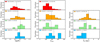 |
Fig. 1. Distribution and mean values of the cluster samples according to the main parameters studied in this work: M*, Vmax, and Re. The dashed lines depict the mean values for each parameter and sample. For Abell 901/902, no effective radii are publicly available. |
General properties of the cluster and field samples.
2.3. RXJ1347 at z ∼ 0.45
RXJ1347 is a large-scale cluster complex composed of two merging clusters and up to 30 additional infalling groups at z ∼ 0.45 that extend diagonally across the field for about 20 Mpc (Verdugo et al. 2012). This structure is one of the most massive and X-ray luminous clusters known (Schindler et al. 1995). The shocked gas around two very bright galaxies close to the cluster core suggests that RXJ1347 is undergoing a major merger (Verdugo et al. 2012). Our group investigated the internal gas kinematics and star formation activity of a sample of 50 star-forming galaxies in RXJ1347 (Pérez-Martínez et al. 2020). Most of these objects form part of a previous medium-resolution spectroscopic campaign carried out by our group, which allowed us to confirm their cluster membership and star-forming nature. The objects in our sample were distributed around the two main overdensities of the structure, the core of the central cluster (RXJ1347) and another galaxy concentration toward the southeast that coincides with the cluster LCDCS 0825 (Gonzalez et al. 2001). The main physical parameters of these two clusters (M200, R200, and σ, see Lu et al. 2010) are summarized in Table 1.
Our observations with the HR-orange grism of VLT/VIMOS (R ∼ 2500) yielded 19 regular rotating objects with no significant signs of interactions in their rotation curve according to the asymmetry index criterion developed by Dale et al. (2001). In this work, we used this sample of galaxies to study the TFR, VSR, and sAMR in clusters at intermediate redshift. The method we used to obtain the main physical parameters (rest-frame magnitudes, stellar masses, sizes, and rotation velocities) is identical to the method we followed to study the CL1604 sample, and it is described in detail in Sect. 3. The mean properties of this cluster sample, as well as its distribution, are shown in Fig. 1 and listed in Table 3.
2.4. XMM2235 at z ∼ 1.4
XMM2235 is one of the most massive and X-ray emitting virialized clusters found at z > 1 (Mullis et al. 2005; Rosati et al. 2009; Jee et al. 2009). Even though high-redshift clusters tend to be dominated by blue star-forming galaxies even in their cores (Butcher-Oemler effect, Butcher & Oemler 1978), XMM2235 has a tight red sequence and a prominent BCG in its center, indicating that this cluster may be in an advanced evolutionary stage in terms of formation of its stellar populations and the assembly of its mass (Lidman et al. 2008; Strazzullo et al. 2010). This is also confirmed by the high M200 and σ values computed for this cluster through weak lensing (Jee et al. 2009, see Table 1).
Our group carried out slit spectroscopic observations with VLT/FORS2 (R ∼ 1400) to study the gas kinematics of 27galaxies within the cluster environment. Our target selection was based on the previous spectrophotometric campaigns carried out by Rosati et al. (2009) and Strazzullo et al. (2010), as well as in the Hα narrow-band survey conducted in this field by Grützbauch et al. (2012). We successfully recovered regular rotation curves for six cluster members and studied different scaling relations such as the TFR and the VSR (Pérez-Martínez et al. 2017). Our sample is composed of relatively compact massive objects with stellar mass and size mean values equivalent to log M* = 10.5 ± 0.1 and Re = 3.3 ± 0.5 kpc, respectively (see Fig. 5 and Table 3). Further details about the analyses of this sample can be found in Pérez-Martínez et al. (2017).
2.5. HSC-Cl2329 and HSC-Cl2330 at z ∼ 1.47
These clusters were identified as strong [OII] overdensities by exploiting the narrow-band filter NB921 in the HSC-SSP 16 deg2 emission-line survey (Hayashi et al. 2018b) and not by X-ray observations or red-sequence detection. They are dominated by star-forming galaxies and are more typical progenitors of the current regular population of clusters. Therefore these HSC clusters offer a window for testing the properties of galaxies during the cluster assembling process. Our group carried out 3D spectroscopy with KMOS (R ∼ 4000) at the VLT for both structures, confirming the membership of 34 objects and extracting regular velocity fields for 14 objects, which were used to explore the B-band TFR at this redshift (Böhm et al. 2020). Based on the low velocity dispersion and the large projected size of the protoclusters, Böhm and collaborators argued that these structures are not yet virialized. However, they were unable to compute stellar masses because not enough photometric bands covered the rest-frame redder part of the spectral range. Similarly, the point spread function (PSF) size from the HSC images matches the expected effective radius of galaxies at this redshift, which makes any attempt to determine the galaxy size unreliable. We therefore restricted the use of this sample to the analysis of the cluster B-band TFR at different epochs. For a more detailed description of the cluster detection and target properties, we refer to Hayashi et al. (2018b) and Böhm et al. (2020).
2.6. Field comparison samples
In this section, we briefly introduce the main properties of the field comparison samples we used in our analysis. Our primary comparison sample is composed of 124 field galaxies at z < 1 from Böhm & Ziegler (2016). These galaxies were selected from the FORS Deep Field (Heidt et al. 2003) and the William Herschel Deep Field (Metcalfe et al. 2001). Reliable rotation velocities, B-band absolute magnitudes, and galaxy sizes were computed for these objects following the same methods applied to our cluster sample, which are described in Sect. 3. We used this sample in the context of the evolution of the B-band TFR and VSR, but we excluded it from the sAMR because we lack reliable stellar mass values.
We also selected several kinematic studies with reliable values of angular momentum as comparison samples at different redshifts. The first sample was taken from Fall & Romanowsky (2013, 2018). The authors studied the specific angular momentum of galaxies of varying morphology at z = 0, finding parallel sequences for the different Hubble types. We restricted our comparison sample to objects whose bulge-to-disk ratio is lower than 0.3, which according to the authors ensures the selection of late-type galaxies (Sa to Sd). After this selection criterion was applied, this subsample was composed of 44 disk galaxies within the range 9.0 < log M* < 11.2 for individual objects. Measurements in the local universe establish a zero-point to any scaling relation evolutionary path across cosmic time. To ensure that we were able to reliably fix this zero-point, we included a second local universe comparison sample by Posti et al. (2018), who revisited previous z = 0 studies on angular momentum using a subsample of 92 nearby galaxies from the SPARC survey (Lelli et al. 2016). We followed the same late-type selection criteria as we applied to the Fall & Romanowsky (2013, 2018) sample and removed 16 galaxies with S0, irregular, or compact morphology. This left a subsample of 76 spiral galaxies with stellar mass values of 8.0 < log M* < 11.2.
Our third field comparison sample is composed of galaxies from the KROSS survey (Stott et al. 2016) at z ∼ 0.9. Our selection criteria follow the approach of Harrison et al. (2017) in their angular momentum study but add tighter constraints. We decided to use only galaxies that are rotationally supported (i.e., Vrot/σ > 1) and with well-determined effective radius and inclination angles from imaging data (i.e., quality 1 in Harrison et al. (2017)). In addition, we discarded galaxies whose inclination angles are lower than 25° due to the high systematic errors that small variations in this parameter may introduce in the determination of the rotation velocity. After this, the KROSS sample is made of 301 objects within a mass range of 8.7 < log M* < 10.0.
At high redshift, we used the KMOS Galaxy Evolution Survey (KGES, Gillman et al. 2020) and the SINS/zC-SINF survey (Förster Schreiber et al. 2018) to explore the angular momentum evolution of field galaxies. The first sample is composed of 25 main-sequence star-forming disk galaxies at z ∼ 1.5 published in Gillman et al. (2020). These galaxies display a mass range given by 9.5 < log M* < 11.1. The SINS sample was originally composed of 35 galaxies from which we removed 7 objects because of their irregular morphological classification and their insufficient rotational support (i.e., Vrot/σ < 1). We discarded another 3 objects because their redshift (z ∼ 1.5) is far lower than that of the rest of the sample. Thus, we created a sample of 25 star-forming disk galaxies at 2 < z < 2.5 with stellar masses in the range of 9.3 < log M* < 10.5.
While the stellar mass range of our cluster samples at intermediate to high redshift is cut off at log M* = 9.5, the field galaxy samples previously introduced display a significant population of galaxies below this threshold, even down to log M* = 8.0 for the local studies. The absence of this type of galaxies arises because the size of our cluster observing programs is moderate compared to some of the field studies, and because it is difficult to detect and extract kinematic information from low-luminosity low-mass objects, especially in the outer parts of a rotation curve. To solve this problem, we restricted our subsequent comparative analysis between the cluster and field samples to galaxies above log M* = 9.5. The distribution of our field comparison samples with respect to their M*, Vmax, and Re after this mass cut was applied is shown in Fig. 2, and their mean values are summarized in Table 3. We note that the mean and median values for these three parameters agree within their typical errors (i.e., 0.1 dex for log(M*), 30 km s−1 for Vmax, and 0.3 kpc for Re) for both our cluster and field comparison samples at similar redshift.
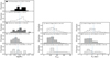 |
Fig. 2. Distribution and mean values of the field samples according to the main parameters studied in this work: M*, Vmax, and Re. The dashed lines depict the mean values for each parameter and sample. No effective radii and rotation velocity are publicly available for the samples of Fall & Romanowsky (2018), Posti et al. (2018), and Gillman et al. (2020), while there are no stellar mass values available for Böhm & Ziegler (2016). |
3. Parameters of CL1604 galaxies
3.1. Rest-frame magnitudes and stellar masses
We used the SED fitting code LEPHARE (Ilbert et al. 2006; Arnouts & Ilbert 2011) to compute the rest-frame magnitudes and stellar masses in our cluster sample. For every object, LEPHARE fits the SED given by the available photometric bands to a library of stellar population synthesis models (Bruzual & Charlot 2003) assuming Calzetti’s attenuation law (Calzetti et al. 2000). We constrained the models to use extinction values of E(B − V) = 0−0.5 mag in steps of 0.1 mag, and to produce galaxy ages younger than the age of the Universe at z ∼ 0.9 (i.e., 6.2 Gyr) assuming a Chabrier IMF (Chabrier 2003). Our rest-frame magnitudes and logarithmic stellar masses are computed in this way to an accuracy of 0.1 magnitudes and 0.15 dex. To study the redshift evolution of the TFR in Sect. 4, we corrected the derived absolute B-band magnitudes for extinction due to the inclination angles of the galaxies with respect to the line of sight. In edge-on spirals, the stellar light has to travel through the galaxy disk, which is filled with dust particles, before it reaches us. Therefore these galaxies possess higher extinction values than their face-on counterparts. In addition, more massive galaxies have higher dust content than low-mass objects (Giovanelli et al. 1995), which introduces a stellar mass dependence in the inclination extinction correction. We took these two effects into account following the prescription given by Tully et al. (1998). This correction diverges for completely edge-on galaxies (i.e., i ≈ 90°), and therefore we excluded them from our sample. After this correction was applied, the typical errors for the B-band absolute magnitude values for the CL1604 sample are ∼0.2 mag.
3.2. Structural parameters
Space-based HST observations are ideal for measuring the structural parameters of our targets reliably due to their high spatial resolution and depth. The field in which CL1604 resides is covered by extensive HST imaging in two filters (F606W and F814W) that covers most of the structure of the cluster complex, including all but one of our targets. In general, images taken in redder filters capture the light from the old stellar population that dominates the structure of the galaxy, which diminishes the contamination coming from prominent star-formation regions. We chose the F814W images as the main source to measure the structural parameters of our cluster members for this reason. We also used the HSC z-band to make the same measurements over the single object that has no HST imaging due to the depth and seeing conditions (full width at half maximum, FWHM, ∼0.5″) achieved in this band during the observations.
We modeled the surface brightness profile of our targets and measured their structural parameters using the GALFIT code (Peng et al. 2002). The models were produced following a two-component approach: first, we fit a single-component exponential profile (Sérsic index ns = 1) to every galaxy and subtracted it from the original image. After visually inspecting the residuals, we determined whether the object under scrutiny showed signs of a bulge. When this was not the case, we kept the structural parameters that were computed with a single exponential disk surface brightness profile. However, when strong residuals were visible in the central areas of the galaxy, we proceeded with a simultaneous two-component fitting by adding another surface brightness profile with n = 4 to take the bulge contribution into account while keeping the single-component results as the initial guess values for the first component.
The modeling provided us with the position angle of our objects (θ) with respect to north, the effective radius (Re) of the disk component, and the ratio between the apparent minor and major axis (b/a). The position angle can be used to identify possible misalignments between the major axis of the galaxy and its slit. This quantity is called the mismatch angle (δ) and was used at a later stage to correct the observed rotation velocities of our targets. The ratio between the axes, b/a, can be used to compute the inclination (i) of the galaxy with respect to the line of sight, which also plays an important role in the determination of the maximum rotation velocity. Finally, spiral galaxies have a small but significant scale height (q) that enters in the determination of i following the approach given by Heidmann et al. (1972), s
 (1)
(1)
where q = 0.2 represents the typical observed value for local spiral galaxies (Tully et al. 1998). The three clusters that belong to our primary sample (RXJ1347, CL1604, and XMM2235) rely on Re measurements from different filters and at different redshifts. However, de Jong (1996) found that the effective radius of disk galaxies varies significantly with wavelength. Kelvin et al. (2012) measured a reduction of 25% in Re for late-type galaxies from g to K band, and established a relation accounting for these changes using measurements from the GAMA survey,
 (2)
(2)
where λrest is the observed rest-frame wavelength for the galaxy. We used this relation to normalize the Re measurements of our three galaxy clusters to the same reference wavelength, λref ∼ 8100 Å. This value is the rest-frame central wavelength of the I-band Johnson filter, which was used to characterize the local VSR in Haynes et al. (1999b) and by Böhm & Ziegler (2016) for their z < 1 field sample of galaxies. After we applied this correction, the effective radius of the galaxies decreased by ∼10% for the RXJ1347 sample (observed with SUBARU Suprime-Cam/z′ at z ∼ 0.45) and by ∼19% for the CL1604 sample (observed with HST/F814W at z ∼ 0.9), while it increased to ∼5% for the XMM2235 sample (observed with HAWKI/K-band at z ∼ 1.4). Our previous analysis of HST/ACS images of disk galaxies reported systematical errors of 20% in galaxy sizes (Böhm et al. 2013; Pérez-Martínez et al. 2020). We also adopted this error value for our work below.
3.3. Determining the maximum intrinsic velocity (Vmax)
Our approach for extracting rotation curves from prominent emission lines and the subsequent modeling for determining the maximum rotation velocity (Vmax) has been extensively described in previous publications of our group (see Böhm et al. 2004; Bösch et al. 2013b; Böhm & Ziegler 2016). However, we provide a summary of the most important steps of the process in the following paragraphs.
First, we find our prominent spectral feature within the 2D spectra ([OII]3727 Å for CL1604)) and measure the central wavelength position of the emission line by fitting a Gaussian profile over it row by row. We average the emission line over three neighboring rows (i.e., 0.75″ in the spatial axis) to enhance the signal-to-noise ratio (S/N) before the fitting. For every row, we inspect the small blue- and redshifts of the central wavelength position in the dispersion axis and transform them into positive and negative velocities with respect to the systemic velocity at the center of the galaxy. In this way, we obtain a position-velocity diagram that displays the rotation velocities as a function of galactocentric radius. We allow for small variations between the photometric and kinematic center of the galaxy of up to ±1 pix, that is, ∼2 kpc in spatial scale at z ∼ 0.9.
The second step of the process involves the correction of the position-velocity diagram from all observational (beam-smearing) and geometrical effects (inclination, misalignment angle, and slit width) that may affect the observed values. To solve this, we generate synthetic velocity fields assuming an intrinsic rotation law, taking into account the seeing conditions at the time of the observations and the structural parameters previously determined through surface brightness modeling. We follow the multiparametric rotation law presented in Courteau (1997), which is characterized by a linear rise at distances smaller than the turnover radius (rt) and a constant maximum rotation velocity (Vmax) beyond this point, where the dark matter halo dominates the mass distribution. Finally, we place a slit along the major axis of the object and extract the synthetic rotation velocity values from the model as a function of radius. These values define a synthetic rotation curve that is allowed to change by tuning the Vmax and rt to fit (via χ2 minimization) the observational shape directly extracted from the 2D spectra. The precision achieved in the determination of Vmax is mainly affected by the accuracy of the structural parameters (especially i) and the quality and extent of the rotation curve, with typical error values of about 20−30 km s−1. In CL1604, only eight regular rotation curves could be extracted out of 34 observed cluster objects, 12 of which displayed irregular kinematics. The remaining galaxies showed just gradients or too compact emission to asses their kinematic state. The synthetic and observed rotation curves can be found in Appendix A for Cl1604 cluster members. The same information is available for XMM2235 and RXJ1347 in our previous publications (Pérez-Martínez et al. 2017, 2020).
3.4. Star formation activity
Between the wide variety of star formation diagnostics available from different emission lines, the Hα prescription developed by Kennicutt (1992) has proven to be one of the most reliable (Moustakas et al. 2006). However, in the intermediate-to-high redshift regime, the access to the Hα emission line can only be achieved through near-IR observations. The three clusters that form part of our cluster primary sample (i.e., RXJ1347, CL1604, and XMM2235) only have spectroscopy in the optical wavelength range, which forces us to use a different calibration. The [OII] emission line doublet at 3727 Å has also been used as a proxy to estimate the SFR of galaxies by empirically calibrating this indicator with respect to the Hα diagnostic (e.g., Verdugo et al. 2008). However, the [OII] calibration is subject to significant uncertainties related to the chemical evolution of galaxies, the dust reddening, and the ionizing process of star-forming galaxies (Moustakas et al. 2006; Kennicutt & Evans 2012). All these effects are of special importance when galaxies at high redshift are examined because the available information in the rest-frame optical wavelength range only covers the bluer parts of the galaxy spectra. Despite these caveats, we used the SFR[OII] diagnostic outlined in Kennicutt (1992) to roughly estimate the SFR of our sample:
![Mathematical equation: $$ \begin{aligned} {SFR}_{[\mathrm OII]}/(M_{\odot }\,\mathrm{yr}^{-1})=2.7\times 10^{-12}\frac{L_B}{L_{B,\odot }}EW([\mathrm{OII}])E(\mathrm{H} {\alpha }) ,\end{aligned} $$](/articles/aa/full_html/2021/02/aa36456-19/aa36456-19-eq6.gif) (3)
(3)
where (LB/LB, ⊙) = 100.4(MB − MB, ⊙), MB, ⊙ = 5.48 mag, EW([OII]) is the equivalent width of the [OII] emission line and E(Hα) is the extinction around Hα. We estimated the value of this quantity by assuming a Calzetti et al. (2000) extinction law, a Chabrier (2003) IMF, and taking the E(B − V) reddening value obtained from the stellar continuum SED fitting (see Sect. 3.1), which accounts for the diffuse dust attenuation in the galaxy (Acont). However, this value should be corrected by adding an additional contribution to the attenuation coming from the active star-forming regions (Aextra). We followed the approach outlined in Wuyts et al. (2013), who studied the dust attenuation of galaxies at 0.7 < z < 1.5 and reported that  , in good agreement with the previous estimates made by Calzetti et al. (2000) in the local universe.
The SFR and E(B − V)SED values of our primary cluster sample can be found in Tables A.1–A.3. The [OII] emission line did not enter the observed wavelength range for three objects in the RXJ1347 sample. These objects were excluded from all diagrams involving SFR. Kennicutt (1992) estimated that the systematic uncertainty of using the [OII] calibration ranges from 30% for local and low-redshift samples to up to a factor 2–3 (0.3–0.5 dex) at high redshift. We display the specific star formation (sSFR) of our cluster samples in Fig. 3 using the main sequence (Eq. (1) in Peng et al. 2010) at the redshift of our clusters as a reference for the expected sSFR value in the field with an scatter equivalent to 0.3 dex (gray area). Most of our objects show sSFR values that are compatible with those of the main sequence in the field within the errors.
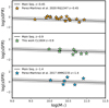 |
Fig. 3. Star formation activity as a function of stellar mass. Orange, green, and blue stars display cluster galaxies within RXJ1347, CL1604, and XMM2235, respectively. The solid line shows the main sequence of star-forming galaxies at z ∼ 0.45, z ∼ 0.90, z ∼ 1.4 extrapolated by Peng et al. (2010), and the gray area indicates the 3σ scatter. |
3.5. Environment
We investigated the effects of the environment on several kinematic scaling relations and their redshift evolution. To this aim, we studied the main kinematic and structural parameters of several cluster samples across cosmic time in previous sections. However, cluster membership in all these samples is usually defined as an interval in redshift space around the value given for the whole cluster structure, which usually coincides with its BCG. Even though this may be sufficient to qualitatively separate the general field population of galaxies from objects residing in denser environments, we need a quantitative way to measure the environment in order to study its effect within these dense regions.
The environment can be quantified in two different ways: locally, as a number density of cluster members (e.g., Dressler 1980); and globally, by taking into account the general properties of the cluster (M200, R200, and σ) to define its phase-space (Carlberg et al. 1997). While the first case requires a high number of known spectrophotometric cluster members to create a homogeneous mapping of each structure, the second case relies on the projected clustercentric distance (Rproj) of each object and its relative line-of-sight velocity with respect to the systemic velocity of the cluster (Δv), which can be measured through the redshift of each object. We chose this second approach for our study given the heterogeneous origin of our samples, which prevents us from conducting a systematic study of the local environmental conditions within each cluster. We followed the approach outlined by Noble et al. (2013), who used a parameter (η) that defines caustic profiles in a phase-space diagram in the following way:
 (4)
(4)
where |Δv| = |(z−zcl) c/(1+zcl)| and zcl is the redshift of the cluster. Attending to this parameter, Noble et al. (2013) defined three separate regions: η < 0.4 for galaxies in the virialized region of the system, 0.4 < η < 2 for galaxies that have recently been accreted, and η > 2 for galaxies that are not yet associated with the main structure of the cluster. However, this scheme only traces the environment within virialized clusters, while other minor cluster-related substructures such as filaments or infalling groups cannot be accounted for. We therefore decided to use η as a continuous parameter that models the environmental relation of a given galaxy to a large cluster (according to Table 1) while keeping the objects with η > 2, as they may form part of some minor substructures in the outskirts of the clusters. We display the environmental (η) distribution of our primary sample in Fig. 4 and the individual values are shown in Tables A.1–A.3 for each cluster. The mean η values of each sample are equal to 3.5 ± 1.0, 2.2 ± 0.7, and 3.3 ± 1.0 for RXJ1347, CL1604, and XMM2235, respectively.
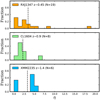 |
Fig. 4. Global environment distribution of galaxies for RXJ1347, CL1604, and XMM2235 clusters. The η value of each object has been computed according to its nearest cluster in Table 1. The dashed line displays the mean value of each sample. |
4. Results
The rotation velocity, the galaxy size, and the luminosity (or stellar mass) comprise a multiparametric space which can be projected onto several planes to produce scaling relations that are key to understanding the evolutionary processes of disk galaxies. We used the cluster and field samples introduced in Sect. 2 to study the evolution of the B-band TFR, VSR, and sAMR with respect to environment and time. In the first two cases, we focus on samples that were exclusively studied by our group to achieve full consistency in the method that was used to extract the main physical parameters of the datasets. For the angular momentum, on the other hand, we chose additional comparison field samples from the literature that provide the parameters we need to study them (i.e., M*, Re, and Vmax).
4.1. B-band Tully-Fisher relation
First, we examined the distribution of our targets in the B-band Tully-Fisher diagram (Fig. 5, left-hand panel). Cluster objects are plotted using stars following the color scheme of previous figures to express their membership to different clusters. We used the local TFR (solid black line, Tully et al. 1998) and a sample of 124 field disk-like galaxies from Böhm & Ziegler (2016) at 0.1 < z < 1 for comparison. The gray area in Fig. 5 depicts the distribution of the field sample around the local relation. Its half-width is equal to three times the scatter of the distribution (3σf), which encompasses the majority of the field galaxies.
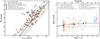 |
Fig. 5. Left: B-band TFR. Colored stars represent the different cluster samples that compose our study. The solid black line shows the local B-band TFR (Tully et al. 1998) with a 3σ scatter area reported by Böhm & Ziegler (2016) for galaxies at 0 < z < 1 (gray area). Right: B-band TFR offset evolution. Stars with colored edges represent the distribution of our cluster samples, and their respective mean values are shown as larger circles of the same color. Error bars represent the error of the mean for every sample. Open circles display the Böhm & Ziegler (2016) field sample at 0.1 < z < 1. We binned the field sample into three redshift intervals (0 < z < 0.33, 0.33 < z < 0.66, and 0.66 < z < 1). Black circles depict the mean value and its error for the field sample in every redshift window. The dashed line represents the predicted B-band luminosity evolution by Dutton et al. (2011) in the TFR, and the dash-dotted line at ΔMB = 0 means no size evolution. |
Most cluster galaxies lie within the 3σf field distribution, although at a fixed rotational velocity, the objects progressively move toward higher B-band absolute magnitudes with redshift. This is a natural consequence of the gradual evolution of the stellar populations with lookback time: higher SFRs and younger (and hotter) stars contribute more to the luminosity of the galaxy when the universe was at an earlier stage. This effect is also shown in the right-hand panel of Fig. 5, where we display the B-band magnitudes offsets from the local TFR (ΔMB = MB, z − MB, z = 0) as a function of redshift. Because our samples have large scatter, we also plot the mean offset values of our cluster datasets and their errors. We followed a similar approach for the field sample by splitting it into three redshift bins (z < 0.33, 0.33 < z < 0.66, and 0.66 < z < 1.0). The mean B-band TFR offset value ( ), the error of the mean (
 ), and the dispersion (σΔMB) for every sample are listed in Table 4.
Summary of the TFR and VSR properties of the cluster and field samples.
Our results show a gradual increase in ΔMB for cluster galaxies up to z ∼ 1 (colored circles, ΔMB ≈ −1). This trend is replicated by the binned mean values for field galaxies from Böhm & Ziegler (2016) (empty circles), which account for the same redshift intervals, but with larger number statistics. Although the field mean values tend to lie slightly below those of the clusters, this small difference becomes negligible when the errors of the mean are taken into account. On the other hand, the semianalytical model by Dutton et al. (2011) (dashed line) predicts a rise in B-band luminosity that is compatible with our results in the cluster and in the field at a similar redshift. This model is based on evolving dark matter halos that host baryonic disks in their centers. The evolution of the stellar mass and gas content of the disks is driven by the radial variation of star-formation, gas recycling, and accretion, which are the main processes that affect the evolution of galaxies in the field (Peng et al. 2010). Thus, our results indicate that the environment has little to no effect on cluster galaxies with regard to the B-band TFR up to z ∼ 1. However, the two higher redshift cluster samples significantly deviate from the semianalytical predictions at the 1.6σ level for XMM2235 (ΔMB = 1.57 ± 0.41) and at the 4.2σ level for the two HSC clusters (ΔMB = 2.18 ± 0.30). Unfortunately, we do not have a field comparison sample that was analyzed following the methods described in Sect. 3 at this high redshift. Nevertheless, this behavior indicates that unaccounted-for processes affect the B-band luminosity of high-redshift cluster galaxies.
4.2. Velocity-size relation
Galaxies are smaller at higher redshifts (Bouwens et al. 2004). This is a consequence of the growth of disks across cosmic time, and it is one of the predictions of the hierarchical growth of structures (Mao et al. 1998). By construction, our cluster samples are exclusively made of disk galaxies (see Sect. 3). Therefore the disk scale length (Rd) can be used to investigate the size evolution of our cluster samples in the VSR. Our results are shown in the left-hand diagram of Fig. 6, which follows the same symbol scheme as used in the TFR, but now marks the local velocity-size relation from Haynes et al. (1999a) with a solid line. Galaxies from Abell 901/902 at z ∼ 0.16 and from the two HSC clusters at z ∼ 1.5 are excluded because we lack size measurements in their respective parent studies (Bösch et al. 2013a; Böhm et al. 2020). In general, the disk size correlates with the wavelength at which it is observed; bluer wavelengths yield higher Rd (Kelvin et al. 2012; van der Wel et al. 2014). Even though Rd was originally measured using different photometric bands for every sample, we used Eq. (2) to renormalize all size measurements to the same rest-frame wavelength and compared our results with the field reference sample of Böhm & Ziegler (2016).
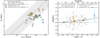 |
Fig. 6. Symbols and color schemes are the same as in Fig. 5. Left: velocity-size diagram. The solid black line shows the local VSR from Haynes et al. (1999a), with a 3σ scatter gray area around it. Right: velocity-size offset evolution. |
As for the TFR, we explored the redshift evolution of the VSR in the right-hand diagram of Fig. 6 and compared our results once again with the semianalytical models of Dutton et al. (2011). Interestingly, we find that cluster and field galaxies have a similar average size evolution, with a factor 1.6 drop in size (Δ log Rd = −0.20 ± 0.07 for CL1604) by z ≈ 1. This result agrees with the predictions of Dutton et al. (2011), although individual objects display large scatter around the mean. This may be related to the different formation ages of galaxies and their distinct evolutionary paths. Observational studies in the field such as van der Wel et al. (2014) reported that the size growth of disk galaxies with redshift is given by Re ∝ (1 + z)−0.75, which yields a factor 1.6 growth between z = 1 and z = 0 at a fixed stellar mass, confirming our previous results. However, this empirical relation only predicts a factor 2 growth at z = 1.5, in agreement with Dutton et al. (2011), but in contrast with our results in XMM2235, which shows smaller sizes by almost a factor 3 (Δ log Rd = −0.46 ± 0.12). The mean offsets with respect to the VSR ( ), the error of the mean (
 ), and the dispersion (σΔ log rd) for every sample are listed in Table 4.
4.3. Angular momentum
The angular momentum (J) simultaneously connects all the relevant parameters involved in the previous scaling relations, that is, stellar mass, size, and rotation velocity. The transference of angular momentum from the dark matter halo to the baryonic component is key to understanding the early stages of galaxy formation (Mo et al. 1998). On the other hand, the stellar specific angular momentum defined as j* = J/M* has proven to be a fundamental quantity for exploring galaxy evolution and morphological transformation. Fall (1983) first found a tight relation between j* and M* with the form  . Its normalization depends on the galaxy morphological type, with parallel sequences toward lower j* values for early-type galaxies, indicating that a loss of angular momentum of up to an order of magnitude is linked to the morphological evolution of galaxies (Romanowsky & Fall 2012; Fall & Romanowsky 2013, 2018). In this section we compare the results obtained for the sAMR (i.e., j* − log M*) for cluster and field galaxies at different epochs. To maintain consistency between the analysis of our cluster and field samples, we adopted the theoretical frame described in Harrison et al. (2017) to study the evolution of angular momentum, for which we present a summary in the following paragraphs. First, Eq. (6) in Romanowsky & Fall (2012) was used as an estimate for j*,
 (5)
(5)
where Re is the effective radius of the galaxy, vs is the observed rotation velocity at some arbitrary radius, Ci is an inclination correction factor, and kn is a numerical factor that takes into account the current morphology of the galaxy approximated by its Sérsic index (n) in the following way:
 (6)
(6)
By construction (see Sect. 3.2), our samples only contain disk galaxies so that they display characteristic exponential surface brightness profiles (n ∼ 1). Furthermore, small variations of n in the vicinity of the exponential profile (e.g., 0.5 < n < 1.5) will only introduce small variations in the value of kn (up to 7%). Therefore we confidently assumed n = 1 as our standard value for all further calculations, adding such uncertainty contribution to the j* error budget. Additionally, we may consider that our inclination and seeing-corrected maximum rotation velocity is equivalent to Vmax ≈ Civs, simplifying Eq. (5) for disk galaxies to just
 (7)
(7)
where Rd is the disk scale length and Rd ≈ Re/1.678. This approach converts the sAMR into a correlation between two independent variables, j* and M*. In Fig. 7 we present the results obtained for our cluster galaxies in comparison to our selection of field samples, which were analyzed following the same method as described above. The distribution of the local data is fit by the expectations for disks given by Fall & Romanowsky (2013) (blue line). At higher redshifts, the field and the cluster samples display lower j* values but seem to follow sequences with similar slope. However, the scatter of our data and the limited number statistics of the cluster members prevent us from computing a slope value that could be used as a comparison between the cluster and field samples at different redshifts.
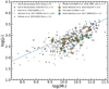 |
Fig. 7. Specific angular momentum diagram. Orange, green, and blue stars represent the RXJ1347, CL1604, and XMM2235 cluster galaxies, respectively. Black and empty circles show the local universe disk-like samples from Fall & Romanowsky (2018) and Posti et al. (2018), respectively. The small black crosses show the field objects from the KROSS sample at z ∼ 0.9 (Harrison et al. 2017), empty diamonds display the KGES sample at z ∼ 1.5 (Gillman et al. 2020), and the gray squares depict SINS/zC-SINF galaxies at z ∼ 2 (Förster Schreiber et al. 2018). The solid blue line displays the local “Fall relation” for disk galaxies from Fall & Romanowsky (2013). |
To further explore the possible variations in j* as a function of redshift and environment, Harrison et al. (2017) applied a simple predictive model based on the works of Romanowsky & Fall (2012) and Obreschkow & Glazebrook (2014) (their Eqs. (18) and (19)), assuming that the baryonic fraction can be approximated by fb = 0.17 (Komatsu et al. 2011),
![Mathematical equation: $$ \begin{aligned} \frac{j_{*,\mathrm{pre}}}\mathrm{kpc\,km\,s^{-1}}=2.95 \times 10^4 f_j f_{\rm s}^{-2/3} \lambda \left(\frac{H[z]}{H_0}\right)^{-1/3} \left[\frac{M_*}{10^{11}M_{\odot }}\right]^{2/3} ,\end{aligned} $$](/articles/aa/full_html/2021/02/aa36456-19/aa36456-19-eq21.gif) (8)
(8)
where H[z]=H0(ΩΛ + Ωm[1 + z]3)1/2. This model relies on the assumptions that all galaxies reside inside singular isothermal spherical cold dark matter halos characterized by a spin parameter λ and a specific angular momentum jh. Therefore the galaxies embedded in such dark matter halos possess a fraction of the specific angular momentum of the halo in which they were formed, fj = js/jhalo. This fraction may change between galaxies from different epochs and evolutionary paths because it represents the specific angular momentum retained by the baryons at a given moment, and this is the focus of our analysis.
During the processes of galaxy formation, the asymmetric collapse of high-density regions generates tidal torques that introduce a particular angular momentum value for every mass distribution (Hoyle 1951; Peebles 1969). The spin parameter accounts for this behavior. N-body simulations and recent observational studies have shown that λ follows a nearly lognormal distribution with an expected value λ = 0.035 and a mean dispersion of 0.2 dex, which remains approximately constant when different epochs, galaxy masses, and environments are examined (Macciò et al. 2007, 2008; Romanowsky & Fall 2012; Bryan et al. 2013; Burkert et al. 2016). Finally, fs represents the stellar mass fraction relative to the initial gas mass. This parameter is a function of the different internal processes that take place within a galaxy as a result of its evolution. Because it is difficult to account for all possible variables involved in the baryonic physics, Harrison et al. (2017) followed an empirical approach and used the mass-dependent description given by Dutton et al. (2010) for late-type galaxies that was revisited in Burkert et al. (2016) for this purpose,
![Mathematical equation: $$ \begin{aligned} f_s=0.29\left(\frac{M_*}{5\times 10^{10}M_{\odot }}\right)^{1/2}\left(1+\left[\frac{M_*}{5\times 10^{10}M_{\odot }}\right]\right)^{-1/2} .\end{aligned} $$](/articles/aa/full_html/2021/02/aa36456-19/aa36456-19-eq22.gif) (9)
(9)
Under these assumptions, the only free parameter in j∗,pre is the specific angular momentum fraction that is retained by the galaxy with respect to its dark matter halo (fj = js/jhalo). We considered the idealized case in which the baryonic and dark matter component of the galaxy have been well mixed from the early stages of galaxy formation, meaning that the specific angular momentum in both components is very similar (js ≈ jhalo), and thus, fj ∼ 1. In Fig. 8 we present the discrepancies between j∗,pre (assuming fj = 1) and the values computed following Eq. (5) for all the cluster and field galaxies (i.e., Δlog(j*) = log(j*)−log(jpre)) as a function of stellar mass. This choice of parameters is very useful because the negative values in Δlog(j*) can be reinterpreted as lower fractions of conserved specific angular momentum (i.e., fj < 1) for galaxies that have experienced different conditions (e.g., redshift or environmental evolution). Thus, it provides a way to investigate fj as a function of stellar mass for galaxies with diverse origins.
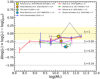 |
Fig. 8. Specific angular momentum offsets (Δlog(j*)) as a function of stellar mass. The solid colored lines depict the mean values and the error of the mean of the mass-binned field samples using bin widths of 0.5 dex. Blue and red lines depict the local universe disk samples from Fall & Romanowsky (2018) and Posti et al. (2018), respectively. The green line shows the distribution of objects from the KROSS sample at z ∼ 0.9 (Harrison et al. 2017). The purple line shows the z ∼ 1.5 KGES sample of galaxies (Gillman et al. 2020), while SINS/zC-SINF galaxies at z ∼ 2 are displayed by the gray line (Förster Schreiber et al. 2018). The dotted lines mark different predicted values of fj as a function of Δlog(j). The light yellow band depicts the predicted scatter in the spin parameter λ assuming fj = 1. The orange, green, and blue circles show the mean Δlog(j)−log(M*) values and their errors for the RXJ1347, CL1604, and XMM2235 cluster galaxies, respectively. Finally, the yellow square displays the average value for Pelliccia et al. (2019) cluster sample. |
In Fig. 8 we show the behavior of the field objects in Δlog(j*) by binning these samples within intervals of 0.5 dex in M*. The solid lines show the resulting mean values and their errors as a function of stellar mass. Objects above Δlog(j*) = 0 (i.e. fj > 1) are allowed to exist in this model because the spin parameter (λ) determination and its mean dispersion value have some uncertainties (0.2 dex, yellow band). We avoided binning our cluster samples because they are poorly sampled in the given mass range. Instead, we simply computed the mean values ( ), errors of the mean (
 ) and dispersion (σΔ log j*) per cluster (colored circles), which are also listed in Table 5.
Summary of the angular momentum properties of the cluster and field samples.
We obtain  for galaxies in RXJ1347 at z ∼ 0.45,
  for galaxies in CL1604 at z ∼ 0.91, and
  for galaxies in XMM2235 at z ∼ 1.39. These three values indicate a significant increase in the angular momentum since z ∼ 1, but little evolution between z ∼ 1 and z ∼ 1.4. As we stated above, we can reinterpret these offsets as a decrease in the retained specific angular momentum fraction, fj, with increasing redshift. Thus, galaxies from RXJ1347 on average conserve 58 ± 5% of their halo specific angular momentum (i.e.,
  ) while the cluster members from CL1604 and XMM2235 on average display
  and
and  respectively. For comparison, we also include the cluster sample that was recently studied by Pelliccia et al. (2019) within the CL1604 multicluster system. Out of the 94 galaxies that are part of their ORELSE-SC1604 sample, only 22 display log(M*) > 9.5, v/σ > 1, and can be considered to be part of the CL1604 cluster system according to the redshift limits imposed by Lemaux et al. (2012) for this structure (0.84 < z < 0.96). We measure
  which corresponds with
  for their sample. These values are compatible with those of the local samples at similar stellar mass (log(M*) = 10.0−10.5 mass bin), where
  for the Fall & Romanowsky (2018) sample and
  for the Posti et al. (2018) sample. In contrast, the results of the KROSS sample at the same mass bin yield
  which implies a 4.2σ difference between the Pelliccia et al. (2019) and the KROSS samples. This gap becomes even larger when we compare it with our high-redshift cluster samples (Cl1604 and XMM2235), although they also display slightly higher mean stellar mass values. This disagreement is maintained even when galaxies with η > 3 are excluded from the 22 selected galaxies within the ORELSE-SC1604 sample. However, Pelliccia et al. (2019) also claimed that methodological differences in their kinematic measurements may not allow a direct comparison of their results with others such as the KROSS survey.
We now compare our results in dense environments at different epochs with the field comparison samples. In the field at z ∼ 0 there is little dependence of Δlog(j*) on the galaxy stellar mass for log(M*) > 9.5. The variations are negligible when the errors of the mean are taken into account for every bin in the local samples (Fall & Romanowsky 2018 in blue and Posti et al. 2018 in red), which display similar average offset values across the mass range under scrutiny. Examining the selected KROSS and KGES disk galaxies at z ∼ 0.9 and z ∼ 1.5 (green and purple bins, respectively) we find a similar situation with no stellar mass dependence but an even lower mean offset across the chosen mass range. Similar results were previously reported in a larger subsample of the KROSS survey by Harrison et al. (2017), who applied less restrictive selection criteria. However, the errors of the KGES sample make it statistically consistent with the field samples in the local universe as well as at z ≈ 1. On the other hand, the z > 2 galaxies from the SINS/zC-SINF survey (Förster Schreiber et al. 2018) display unusual small offsets ( ) compared to the other field z = 1−1.5 samples (KROSS and KGES), but they are consistent with the z = 0 field. This result is at odds with the expectation of j* growth between z = 2 and z = 0 (see Renzini 2020, and references therein). The uncertainties in the measured sizes and morphologies (Sérsic index values) reported in their study may be responsible for this disagreement as the method we used to estimate the specific angular momentum is only valid for disk (n ≈ 1) galaxies. In addition, possible differences between our methods for extracting rotation velocities and those applied to the SINS sample may also contribute to the observed discrepancy.
4.4. Redshift evolution of the angular momentum
In the context of the ΛCDM cosmological model, the specific angular momentum of the dark matter halo depends not only on its mass, but on time (Mo et al. 1998). This dependence scales as  , with n = 1/2 for spherically symmetric halos (Obreschkow et al. 2015). When we assume that the stellar-to-halo mass ratio is essentially insensitive to the redshift evolution (Behroozi et al. 2010), the baryonic component should display a similar behavior
  . These assumptions allow us to investigate the redshift evolution of the specific angular momentum as a function of the environment using the cluster and field samples studied above. In this case, we decided to only use galaxies above log M* = 9.5 for two reasons: first, we showed in Fig. 8 that our field samples at different redshifts have a weak to negligible stellar mass dependence with respect to their j* at log(M*) > 9.5. Moreover, the z ∼ 0 sample from Posti et al. (2018) indicates that in the low stellar mass regime, this dependence may become stronger. In addition, our cluster samples are dominated by relatively massive galaxies (
 ) and lack objects below log M* = 9.5.
We present the sAMR redshift evolution in Fig. 9 after we applied this new constraint. The large symbols represent the mean values and their error for each sample included in our angular momentum analysis. We plot the functional form  for n = 1/2 and n = 1 to allow for different evolutionary paths, and normalized the zero-point (z ∼ 0) to the mean values measured from our local Universe local galaxy samples, which are in remarkable agreement:
  for Fall & Romanowsky (2018) and
  for Posti et al. (2018). It is important to emphasize that these two samples are only composed of spiral galaxies, although they allowed for small variations in the bulge-to-disk ratios (B/D) to include most late-type galaxies. We find that galaxies at higher redshift (KROSS at z ∼ 0.9 and KGES at z ∼ 1.5) follow the scaling of
  well, with lower j* at higher redshift. In particular,
  for the KROSS galaxies and
  for the KGES survey. These values are equivalent to a decrease in j* of a factor 1.3 by z ∼ 1 in comparison to the local spirals, or by a factor 1.6 by z ∼ 1.5, in agreement with the EAGLE numerical simulations (Lagos et al. 2017). On the other hand, the SINS sample at 2 < z < 2.5 is much closer to the local values with
  . A possible explanation for this behavior are the high uncertainties that are reported for the published structural parameters of this sample (i.e., Sérsic index and Re).
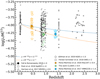 |
Fig. 9. Redshift evolution of j*/M2/3 from z = 0 to z ∼ 2.5. The large black and empty circles show the mean value for the local field galaxies from Fall & Romanowsky (2018) (small black cirles) and Posti et al. (2018) (small empty cirles), respectively. The large empty triangle depicts the average value for the KROSS sample at z ∼ 0.9 (small triangles, Harrison et al. 2017). The empty diamond displays the KGES sample at z ∼ 1.5 (small empty diamonds), and the empty square represents the field galaxies at 2 < z < 2.5 from Förster Schreiber et al. (2018) (small gray squares). The average j*/M2/3 values for the RXJ1347, CL1604, and XMM2235 cluster samples are shown by the orange, green, and blue circles, respectively. The errors of the mean are plotted as error bars for each symbol. The dashed lines represent the expected evolution of the angular momentum with redshift according to the ΛCDM cosmology: j* = M−2/3(z + 1)−n with n = 0.5 (blue) and n = 1 (orange). |
The trend in the cluster samples, on the other hand, is more difficult to interpret. In general, we measure lower  values than in the field, specifically for the higher redshift clusters (e.g., −4.31 ± 0.19 for CL1604 at z ∼ 0.9 and −4.29 ± 0.10 for XMM2235 at z ∼ 1.4, but −4.04 ± 0.21 for RXJ1347 at z ∼ 0.45). Our results suggest that on average, cluster galaxies have a lower j* than their field counterparts at a given epoch. This difference can be explained by the higher probability of interactions that contribute to the angular momentum loss in the cluster environment with respect to the field. Although we do not know the exact contribution of each interaction (e.g., tidal and merging events, ram-pressure stripping, suppression of inflows), these mechanisms appear to be in place as early as z ∼ 1.4 in massive virialized systems such as XMM2235.
5. Discussion
The evolution for nearly isolated galaxies is based on the hierarchical growth of objects and the decline of star formation due to the consumption of gas over cosmic time. However, galaxy clusters strongly affect the evolution of galaxies by introducing cluster-specific interactions that are related to the increasing number density of galaxies toward the central regions of the cluster, the density of the intracluster medium (ICM), and the substructures of the cluster. These interactions can be broadly divided into two classes: hydrodynamical, when the gas component acting as a fluid is mainly affected (e.g., ram-pressure stripping and starvation), and gravitational, when both the stellar and gas component are affected simultaneously by the gravitational potential well of another nearby object (e.g., harassment and mergers). In this section we study the possible contribution of each of these interactions in the evolution of kinematic scaling relations such as the TFR, the VSR, and the sAMR.
5.1. Luminosity and size evolution
Our work on the B-band TFR (see Fig. 5) has shown that cluster galaxies experience a moderate brightening of up to one magnitude between z = 0 and z = 1. This value is compatible with the evolution of field galaxies in the same redshift bin (Böhm & Ziegler 2016) and with the semianalytical model predictions of Dutton et al. (2011), and it suggests that the environment does not play an important role in the B-band luminosity evolution of star-forming galaxies up to this redshift. Therefore this brightening may be mostly driven by the normal evolution of the stellar populations in the galaxies with lookback time. We explore this hypothesis in Fig. 10, where we connect the B-band brightening with the star-formation activity of each object, and with a measurement of the environment they live in through the parameter η.
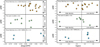 |
Fig. 10. Left: B-band TFR offsets as a function of the sSFR offsets measured from the main sequence of star-forming galaxies (Peng et al. 2010). The color scheme is the same as in previous figures. Right: B-band offsets with respect to the TFR as a function of global environment (η) for galaxies in our cluster samples. The dashed lines indicate log(η) ≈ 0.3, which is equivalent to the boundary between accreted and infalling galaxies according to Noble et al. (2013). |
In the left-hand panel of Fig. 10, we display the B-band TFR offsets as a function of the sSFR offsets measured from the main sequence of star-forming galaxies discussed in Sect. 3.4. We ran a Spearman rank correlation test over the cluster samples included in this diagram. Our results show that even though a negative weak correlation exists between ΔMB and Δ log(sSFR) for RXJ1347 (r = −0.41) and Cl1604 (r = −0.16), their p-values do not allow us to discard the null hypothesis (pRXJ1347 = 0.11 and pCl1604 = 0.69), which is defined by p > 0.05. Thus, we conclude that there is no significant statistical correlation between these parameters for individual cluster galaxies at a fixed redshift. In addition, the right-hand panel of Fig. 10 shows no correlation between the luminosity enhancement and the phase-space position of the objects in RXJ1347 and CL1604 as a function of η. In this diagram η = 2 (i.e., log η ≈ 0.3) divides our galaxy samples into two distinct groups: virialized or recently accreted (η < 2), and infalling (η > 2). The lack of environmental trends between these two groups even when η is used as a continuous parameter within the accreted region suggests that the effect of the environment on ΔMB is probably mild in these samples. Similar results were also found when cluster and field galaxies were compared in the B-band TFR at this redshift by Pelliccia et al. (2019).
There is also no clear correlation between the luminosity enhancements and the sSFR for the XMM2235 objects. However, two out of three objects with the most negative ΔMB values also have very low η values and lie within R500 of their cluster center (see Fig. 1 in Pérez-Martínez et al. 2017). It has been proposed that the early stages of ram-pressure stripping could compress certain regions of the gas disks, causing a temporary enhancement of star formation that results in a moderate rise of the B-band luminosity (up to −0.5 mag) for a given object (Ruggiero & Lima Neto 2017; Ruggiero 2019), while the gas kinematics still shows relatively ordered rotation (Noble et al. 2019). This could partially explain the high B-band luminosity values of these two objects for a given Vmax in the TFR, even though the effects of ram-pressure stripping also depend on the orientation of the disk with respect to the direction of motion within the ICM.
The HSC-protoclusters are structures still in the process of assembling the majority of their mass and building-up their ICM, which makes ram-pressure stripping events unlikely. It has been proposed that during the cluster assembly, galaxies may have higher gas fractions than their field counterparts (Noble et al. 2017; Hayashi et al. 2018a). A possible explanation for this behavior is that the filamentary structure of the cosmic web boosts the inflows of pristine gas toward galaxies at its junctions. We speculate that the channeling of fresh cold molecular gas toward the galaxy disk may be responsible for the creation of small starbursts, which in turn enhance the B-band luminosity of the object. However, this can not be tested with the optical and near-IR data available in these clusters. A simple alternative to the environmentally driven scenarios proposed for XMM2235 and the HSC-protoclusters is that the recipes that govern the star formation activity in the models of Dutton et al. (2011) underestimate the B-band luminosity evolution of TFR objects at high redshift. However, the different evolutionary stages of these structures in terms of mass accretion and dynamical state, together with the low number of objects available for study, do not allow us to draw a decisive conclusion.
We also tested the effect of the environment on the evolution of the disk size through the VSR. We followed the same approach as we applied to the TFR by inspecting the offsets of the VSR (Δ log Rd) with respect to η. We find no statistically significant trend (p ≫ 0.05) between accreted and infalling galaxies in any of our cluster samples (see Fig. 11). However, we find that the two galaxies that are closer to the innermost regions of XMM2235 show sizes that are compatible with the local relation. Even though this may not be a general trend because only a few objects are involved, it does not support the possibility that these galaxies are candidates for ram-pressure stripping because the truncation of the disk is one of the expected changes in this scenario (Crowl & Kenney 2008).
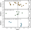 |
Fig. 11. Scale length offsets with respect to the VSR as a function of global environment (η) for galaxies in our cluster samples. The dashed lines indicate log(η) ≈ 0.3, which is equivalent to the boundary between accreted and infalling galaxies, according to Noble et al. (2013). |
5.2. Angular momentum evolution
Several processes may be responsible for the changes in the j* of a galaxy. For example, the outflows of material from the inner parts of a galaxy together with merging events may significantly decrease the j* of an object (Lagos et al. 2018), while the accretion of cold gas in the outskirts of galaxies residing in cosmic web filaments (Danovich et al. 2015) and the migration of clumpy star-forming regions toward the central area of the galaxy may increase it (Dekel et al. 2009).
In the cluster environment, where interactions are more frequent than in the field, the loss of angular momentum may become a more important phenomenon. In a first stage, the hot ICM prevents galaxies from acquiring inflowing material, stopping the buildup of angular momentum that field galaxies experience toward z = 0 (Peng & Renzini 2020). Furthermore, ram-pressure stripping may also remove the outer parts of the disk gas reservoir when galaxies transit the cluster core, causing further angular momentum losses (Romanowsky & Fall 2012). However, this usually requires high ICM density values, which can only be found in the innermost regions of massive clusters. We inspect the fraction of retained angular momentum (fj) as a function of the environment in Fig. 12. The number of objects lying in the virialized regions of the cluster (i.e., log(η) < − 0.4 according to Noble et al. 2013) is small in all our cluster samples, and these objects do not show significantly lower fj values than objects in the recently accreted (−0.4 < log(η) < 0.3) or infalling (log(η) > 0.3) regions. Furthermore, ram-pressure stripping does not seem to play a major role in the luminosity and size evolution discussed in the previous section. These two results suggest that ram-pressure stripping cannot be taken as the main contributor to the loss of angular momentum in our cluster samples, even though it may be acting on a few individual galaxies.
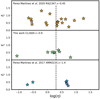 |
Fig. 12. Retained angular momentum fraction (fj) as a function of global environment (η) for galaxies in our cluster samples. The dashed lines indicate log(η) ≈ 0.3, which is equivalent to the boundary between accreted and infalling galaxies, according to Noble et al. (2013). |
The higher object number density in the cluster environment enhances the frequency of close encounters between galaxies compared to the field (Alonso et al. 2012), which may also cause angular momentum exchange and loss through tidal interactions and mergers. While the effects of flyby events might be not as strong as merging events, they may also contribute to increase the loss of angular momentum in dense environments, especially when repeated over time (Moore et al. 1998). On the other hand, the destruction of the galaxy disk through a major merger in the cluster environment would immediately exclude that type of galaxy from our analysis. For example, if the major merger were recent, the disturbed gas kinematics would prevent these objects from being analyzed in any of the scaling relations discussed in this work because we would be unable to derive their Vmax. The descendant of a major merging system may be able to rebuild a disk at a later stage. However, the timescale involved (several billion years, Sparre & Springel 2017) and the need for a significant amount of inflowing gas to build up the new disk (Governato et al. 2009; Sparre & Springel 2017) would not allow these systems to carry out this process inside clusters in most cases, especially taking into account that the inflows are cut by the ICM and the typical quenching timescale is 1−2 Gyr (Wetzel et al. 2013; Maier et al. 2019).
However, minor mergers may be a possible mechanism for the loss of angular momentum within our sample. Depending on the initial conditions of the event (mass ratio, relative velocity, and geometry), minor mergers could locally affect the stability of the disk without fully destroying its structure (Puech et al. 2012). Lagos et al. (2018) investigated the effect of mergers on the specific angular momentum and reported a great variety of behaviors. In general, major mergers will significantly decrease j* (on average by a factor 2–3) after 1 Gyr, with counter-rotating dry mergers being especially efficient in this task. The effects of minor wet and dry mergers after 1 Gyr seem to be more subtle; the former slightly contribute to increase j* by up to a factor 1.25, especially when the merger involves high relative orbital velocities and corotating geometry, and the latter acts in the opposite direction by decreasing j* by a similar amount. In both cases, however, the results strongly depend on the exact gas fractions and the geometry of the event. If minor mergers do play a major role in decreasing j* for cluster galaxies, these interactions should be largely dominated by gas-poor mergers. The average difference between the retained angular momentum fraction of CL1604 and XMM2235 (fj ≈ 0.40) with respect to the KROSS and the KGES (fj ≥ 0.50) samples is about a ∼20%, which is in principle consistent with the decrease predicted by Lagos et al. (2018) as a consequence of minor mergers.
Furthermore, mergers are more likely to occur in the outskirts of the clusters than in their cores (Deger et al. 2018; Bahé et al. 2019), and minor mergers are also more frequent than major mergers in galaxy groups and cluster outskirts (Benavides et al. 2020), as it happens in the field (Lotz et al. 2011; Kaviraj et al. 2015; Ventou et al. 2019). The loss of angular momentum through minor mergers in star-forming galaxies before they reach the cluster core could explain why we do not see significant differences in fj between the population of infalling and accreted cluster regions, as mergers are unlikely to occur in the cluster core, and other angular momentum redistribution mechanisms such as ram-pressure stripping may quench these galaxies rather quickly, excluding them from our samples. However, the small number of objects studied per cluster does not allow us to draw a firm conclusion in this regard. Finally, the gas content and relative position of the velocity vectors of merging galaxies are to a large extent stochastic, and thus it is likely that several events of this nature are required to reproduce the observed offsets between the cluster and field samples. We also emphasize that the contribution by other gravitational cluster-specific interactions (e.g., harassment and flyby encounters) may be as relevant as in the previous case, although it remains unexplored from the numerical simulation point of view to our best knowledge. Larger samples of kinetically analyzed cluster objects are required to shed light onto the role of gravitational interactions as drivers of the angular momentum loss in clusters.
6. Conclusions
We have studied the redshift evolution of the TFR, the VSR, and sAMR in clusters up to z ∼ 1.5. We used a collection of clusters at different redshifts for this purpose, many of which were the single focus of previous publications: Abell 901/902 at z ∼ 0.16 (Bösch et al. 2013a,b), RXJ1347 at z ∼ 0.45 (Pérez-Martínez et al. 2020), XMM2235 at z ∼ 1.4 (Pérez-Martínez et al. 2017), and two HSC (proto-)clusters at z ∼ 1.5 (Böhm et al. 2020). Furthermore, we presented the first results from a sample of galaxies in the CL1604 cluster system at z ∼ 0.9 observed with GTC/OSIRIS. All cluster samples were studied by our group with similar methods and techniques, which make them ideal for a comparative study between different epochs. We also compared our cluster scaling relations with field samples between z = 0 and z = 2.5 (Böhm & Ziegler 2016; Harrison et al. 2017; Fall & Romanowsky 2018; Posti et al. 2018; Förster Schreiber et al. 2018; Gillman et al. 2020), cosmological numerical simulations (Dutton et al. 2010, 2011; Lagos et al. 2017, 2018), and other theoretical works such as Obreschkow & Glazebrook (2014) and Obreschkow et al. (2015). Our main findings are summarized below.
-
Cluster and field galaxies at 0 < z < 1 display similar luminosity brightening in the B-band TFR and generally follow the B-band TFR with increasing B-band luminosity values with lookback time. These results are in agreement with the expectations from semianalytical models by Dutton et al. (2011), who predicted ΔMB ≈ −1 mag by z = 1 due to gradually increasing SFR and younger stellar populations with lookback time. However, we find no correlation between the B-band luminosity enhancement and sSFR within the members of each cluster.
-
Cluster galaxies at z ∼ 1.5 show average B-band luminosity enhancements of ΔMB ≈ 2, deviating from the models of Dutton et al. (2011) by 0.5–1 mag. This behavior is detected for galaxies residing in massive virialized clusters such as XMM2235 and for clusters that are still in the process of assembling the bulk of their mass, such as the two HSC (proto-)clusters studied here. This deviation may be consistent with a moderate underestimation of the modeled luminosity evolution at high redshift. However, based on the conditions of the environment, we cannot completely discard the effect of other processes for individual cases. This includes two galaxies near the center of XMM2235 that may be ram-pressure stripping candidates, and the enhancement of SFR due to higher gas inflows for galaxies in assembling clusters, such as the HSC (proto-)clusters.
-
Our VSR results demonstrate that galaxies decrease their disk sizes with redshift at a fixed rotation velocity. Our cluster and field samples follow very similar trends with an average size decrement of factor 1.6 by z = 1. This result agrees with previous observational constraints (van der Wel et al. 2014) and with the numerical models of Dutton et al. (2011). Galaxies in XMM2235 at z ∼ 1.4 are almost three times smaller than their local field counterparts, slightly deviating from simulations at the same redshift in the field, which predict only a size decrease by a factor of two. However, we find no correlation between the size evolution and η, which argues against environmental effects as the main drivers for this difference within the limitations of this study in terms of number statistics.
-
Cluster galaxies at 0.5 < z < 1.5 follow parallel sequences toward lower j* values in the Fall relation (j* ∝ M2/3Fall 1983; Fall & Romanowsky 2013) with respect to the local field galaxies. The stellar-to-halo specific angular momentum ratio (fj = j*/jhalo) of cluster galaxies at z ∼ 0.45 is 60%, and drops to less than 40% by z ∼ 0.9, and remains constant for XMM2235 at z ∼ 1.4. In contrast, field galaxy samples display ∼20% higher fj values. This may be caused by cluster-specific interactions. We explored the possible contributions of ram-pressure stripping and mergers based on the kinematic study of our cluster samples (TFR, VSR, and sAMR) and suggest that minor mergers may play an important role in angular momentum transformation.
-
Our analysis of the evolution of sAMR with time yielded different trends for galaxies in the field and cluster environments. The ΛCDM model predicts a redshift evolution of j* in the following form:
 (Mo et al. 1998; Obreschkow et al. 2015). We normalized the zero-point of these tracks by reanalyzing the angular momentum contribution of the disk z ∼ 0 galaxies studied in Fall & Romanowsky (2018) and Posti et al. (2018). The mean values for the field samples analyzed in this study follow the predicted trend up to z ∼ 1.5, although they display significant scatter (see Fig. 9). However, cluster samples deviate from this trend at z ≥ 1 and fall onto a path that is better described by
  . This difference suggests that the effects of the cluster environment on angular momentum are in place as early as z ∼ 1.4 in virialized structures, although further work is needed to determine the specific mechanisms that are responsible for this difference.
The search for environmental effects and their relative importance on the physical parameters of the galaxy populations has been a subject of debate during the past 40 years (Dressler 1980). Scaling relations provide us a way to explore these effects from different perspectives. The results of large surveys in the field at intermediate to high redshift, together with new high-precision numerical simulations, give us the perfect tools for establishing reliable comparisons. However, it is still necessary to increase the number statistics of the cluster samples in the same redshift range and investigate their most important parameters in a comprehensive way (i.e., rotation velocity, size, stellar mass and populations, metallicity, etc.) to fully understand the possible environmental effects at play. The use of multiobject IFU observations and cluster-focused new surveys will be of key importance to distinguish the effect of different cluster-specific interactions on the physical properties of galaxies in the next decade.
Acknowledgments
Based on observations made with the Gran Telescopio Canarias (GTC), installed in the Spanish Observatorio del Roque de los Muchachos of the Instituto de Astrofísica de Canarias, in the island of La Palma. This paper is also based on data collected at the Subaru Telescope and retrieved from the HSC data archive system, which is operated by Subaru Telescope and Astronomy Data Center at the National Astronomical Observatory of Japan (NAOJ). The HSC Data analysis was in part carried out with the cooperation of Center for Computational Astrophysics, NAOJ. This work is based in part on observations made with the Spitzer Space Telescope, which was operated by the Jet Propulsion Laboratory, California Institute of Technology under a contract with NASA. This work is based in part on observations made with the NASA/ESA Hubble Space Telescope, obtained from the data archive at the Space Telescope Science Institute. STScI is operated by the Association of Universities for Research in Astronomy, Inc. under NASA contract NAS 5-26555. J.M.P. acknowledges the funding support from the University of Vienna and the Marietta Blau Grant, financed by the Austrian Science Ministry, as well as the support from the Instituto de Astrofísica de Canarias for allowing him to develop his research in their headquarters at the Canary Islands, Spain. H.D. acknowledges financial support from the Spanish Ministry of Science, Innovation and Universities (MICIU) under the 2014 Ramón y Cajal program RYC-2014-15686 and AYA2017-84061-P, the latter one co-financed by FEDER (European Regional Development Funds). This work has been also supported by Dirección General de Investigación Científica y Técnica (DGICYT) grant AYA2016-79724-C4-1-P.
References
- Aihara, H., Arimoto, N., Armstrong, R., et al. 2018, PASJ, 70, S4 [NASA ADS] [Google Scholar]
- Aihara, H., AlSayyad, Y., Ando, M., et al. 2019, PASJ, 71, 114 [CrossRef] [Google Scholar]
- Alonso, S., Mesa, V., Padilla, N., & Lambas, D. G. 2012, A&A, 539, A46 [NASA ADS] [CrossRef] [EDP Sciences] [Google Scholar]
- Arnouts, S., & Ilbert, O. 2011, Astrophysics Source Code Library [record ascl:1108.009] [Google Scholar]
- Asano, T., Kodama, T., Motohara, K., et al. 2020, ApJ, 899, 64 [Google Scholar]
- Bahé, Y. M., Schaye, J., Barnes, D. J., et al. 2019, MNRAS, 485, 2287 [Google Scholar]
- Bamford, S. P., Milvang-Jensen, B., Aragón-Salamanca, A., & Simard, L. 2005, MNRAS, 361, 109 [NASA ADS] [CrossRef] [Google Scholar]
- Behroozi, P. S., Conroy, C., & Wechsler, R. H. 2010, ApJ, 717, 379 [NASA ADS] [CrossRef] [Google Scholar]
- Bell, E. F., Zheng, X. Z., Papovich, C., et al. 2007, ApJ, 663, 834 [NASA ADS] [CrossRef] [Google Scholar]
- Benavides, J. A., Sales, L. V., & Abadi, M. G. 2020, MNRAS, 498, 3852 [CrossRef] [Google Scholar]
- Böhm, A., & Ziegler, B. L. 2016, A&A, 592, A64 [NASA ADS] [CrossRef] [EDP Sciences] [Google Scholar]
- Böhm, A., Ziegler, B. L., Saglia, R. P., et al. 2004, A&A, 420, 97 [NASA ADS] [CrossRef] [EDP Sciences] [Google Scholar]
- Böhm, A., Wisotzki, L., Bell, E. F., et al. 2013, A&A, 549, A46 [NASA ADS] [CrossRef] [EDP Sciences] [Google Scholar]
- Böhm, A., Ziegler, B. L., Pérez-Martínez, J. M., et al. 2020, A&A, 633, A131 [EDP Sciences] [Google Scholar]
- Bösch, B., Böhm, A., Wolf, C., et al. 2013a, A&A, 554, A97 [NASA ADS] [CrossRef] [EDP Sciences] [Google Scholar]
- Bösch, B., Böhm, A., Wolf, C., et al. 2013b, A&A, 549, A142 [NASA ADS] [CrossRef] [EDP Sciences] [Google Scholar]
- Bouwens, R. J., Illingworth, G. D., Blakeslee, J. P., Broadhurst, T. J., & Franx, M. 2004, ApJ, 611, L1 [NASA ADS] [CrossRef] [Google Scholar]
- Bruzual, G., & Charlot, S. 2003, MNRAS, 344, 1000 [NASA ADS] [CrossRef] [Google Scholar]
- Bryan, S. E., Kay, S. T., Duffy, A. R., et al. 2013, MNRAS, 429, 3316 [NASA ADS] [CrossRef] [Google Scholar]
- Burkert, A., Förster Schreiber, N. M., Genzel, R., et al. 2016, ApJ, 826, 214 [NASA ADS] [CrossRef] [Google Scholar]
- Butcher, H., & Oemler, A., Jr 1978, ApJ, 219, 18 [NASA ADS] [CrossRef] [Google Scholar]
- Calzetti, D., Armus, L., Bohlin, R. C., et al. 2000, ApJ, 533, 682 [NASA ADS] [CrossRef] [Google Scholar]
- Carlberg, R. G., Yee, H. K. C., & Ellingson, E. 1997, ApJ, 478, 462 [NASA ADS] [CrossRef] [EDP Sciences] [Google Scholar]
- Cepa, J., Aguiar, M., Escalera, V. G., et al. 2000, in OSIRIS Tunable Imager and Spectrograph, eds. M. Iye, A. F. Moorwood, SPIE Conf. Ser., 4008, 623 [Google Scholar]
- Chabrier, G. 2003, PASP, 115, 763 [Google Scholar]
- Chies-Santos, A. L., Rodríguez del Pino, B., Aragón-Salamanca, A., et al. 2015, MNRAS, 450, 4458 [Google Scholar]
- Contini, T., Epinat, B., Bouché, N., et al. 2016, A&A, 591, A49 [NASA ADS] [CrossRef] [EDP Sciences] [Google Scholar]
- Courteau, S. 1997, AJ, 114, 2402 [NASA ADS] [CrossRef] [Google Scholar]
- Courteau, S., Dutton, A. A., van den Bosch, F. C., et al. 2007, ApJ, 671, 203 [NASA ADS] [CrossRef] [Google Scholar]
- Crawford, S. M., Wirth, G. D., & Bershady, M. A. 2014, ApJ, 786, 30 [NASA ADS] [CrossRef] [Google Scholar]
- Crawford, S. M., Wirth, G. D., Bershady, M. A., & Rand riamampandry, S. M. 2016, ApJ, 817, 87 [Google Scholar]
- Crowl, H. H., & Kenney, J. D. P. 2008, AJ, 136, 1623 [NASA ADS] [CrossRef] [Google Scholar]
- Dale, D. A., Giovanelli, R., Haynes, M. P., Hardy, E., & Campusano, L. E. 2001, AJ, 121, 1886 [Google Scholar]
- Danovich, M., Dekel, A., Hahn, O., Ceverino, D., & Primack, J. 2015, MNRAS, 449, 2087 [NASA ADS] [CrossRef] [Google Scholar]
- de Jong, R. S. 1996, A&A, 313, 377 [NASA ADS] [Google Scholar]
- Deger, S., Rudnick, G., Kelkar, K., et al. 2018, ApJ, 869, 6 [Google Scholar]
- Dekel, A., Sari, R., & Ceverino, D. 2009, ApJ, 703, 785 [Google Scholar]
- Di Teodoro, E. M., Fraternali, F., & Miller, S. H. 2016, A&A, 594, A77 [NASA ADS] [CrossRef] [EDP Sciences] [Google Scholar]
- Dressler, A. 1980, ApJ, 236, 351 [NASA ADS] [CrossRef] [Google Scholar]
- Dutton, A. A., Conroy, C., van den Bosch, F. C., Prada, F., & More, S. 2010, MNRAS, 407, 2 [NASA ADS] [CrossRef] [Google Scholar]
- Dutton, A. A., van den Bosch, F. C., Faber, S. M., et al. 2011, MNRAS, 410, 1660 [NASA ADS] [Google Scholar]
- Fall, S. M. 1983, in Internal Kinematics and Dynamics of Galaxies, ed. E. Athanassoula, IAU Symp., 100, 391 [NASA ADS] [CrossRef] [Google Scholar]
- Fall, S. M., & Romanowsky, A. J. 2013, ApJ, 769, L26 [NASA ADS] [CrossRef] [Google Scholar]
- Fall, S. M., & Romanowsky, A. J. 2018, ApJ, 868, 133 [NASA ADS] [CrossRef] [EDP Sciences] [Google Scholar]
- Förster Schreiber, N. M., Renzini, A., Mancini, C., et al. 2018, ApJS, 238, 21 [NASA ADS] [CrossRef] [Google Scholar]
- Gal, R. R., & Lubin, L. M. 2004, ApJ, 607, L1 [NASA ADS] [CrossRef] [Google Scholar]
- Gal, R. R., Lemaux, B. C., Lubin, L. M., Kocevski, D., & Squires, G. K. 2008, ApJ, 684, 933 [NASA ADS] [CrossRef] [Google Scholar]
- Gallazzi, A., Bell, E. F., Wolf, C., et al. 2009, ApJ, 690, 1883 [NASA ADS] [CrossRef] [Google Scholar]
- Gillman, S., Tiley, A. L., Swinbank, A. M., et al. 2020, MNRAS, 492, 1492 [Google Scholar]
- Gilmour, R., Gray, M. E., Almaini, O., et al. 2007, MNRAS, 380, 1467 [NASA ADS] [CrossRef] [Google Scholar]
- Giovanelli, R., Haynes, M. P., Salzer, J. J., et al. 1995, AJ, 110, 1059 [NASA ADS] [CrossRef] [Google Scholar]
- Gómez-González, V. M. A., Mayya, Y. D., & Rosa-González, D. 2016, MNRAS, 460, 1555 [Google Scholar]
- Gonzalez, A. H., Zaritsky, D., Dalcanton, J. J., & Nelson, A. 2001, ApJS, 137, 117 [NASA ADS] [CrossRef] [Google Scholar]
- Governato, F., Brook, C. B., Brooks, A. M., et al. 2009, MNRAS, 398, 312 [NASA ADS] [CrossRef] [Google Scholar]
- Gray, M. E., Wolf, C., Barden, M., et al. 2009, MNRAS, 393, 1275 [NASA ADS] [CrossRef] [Google Scholar]
- Grützbauch, R., Bauer, A. E., Jørgensen, I., & Varela, J. 2012, MNRAS, 423, 3652 [NASA ADS] [CrossRef] [Google Scholar]
- Gunn, J. E., Hoessel, J. G., & Oke, J. B. 1986, ApJ, 306, 30 [Google Scholar]
- Hall, M., Courteau, S., Dutton, A. A., McDonald, M., & Zhu, Y. 2012, MNRAS, 425, 2741 [NASA ADS] [CrossRef] [Google Scholar]
- Harrison, C. M., Johnson, H. L., Swinbank, A. M., et al. 2017, MNRAS, 467, 1965 [NASA ADS] [CrossRef] [Google Scholar]
- Hayashi, M., Tanaka, M., Shimakawa, R., et al. 2018a, PASJ, 70, S17 [NASA ADS] [Google Scholar]
- Hayashi, M., Tadaki, K.-I., Kodama, T., et al. 2018b, ApJ, 856, 118 [NASA ADS] [CrossRef] [Google Scholar]
- Hayashi, M., Koyama, Y., Kodama, T., et al. 2019, PASJ, 71, 112 [Google Scholar]
- Haynes, M. P., Giovanelli, R., Salzer, J. J., et al. 1999a, AJ, 117, 1668 [NASA ADS] [CrossRef] [Google Scholar]
- Haynes, M. P., Giovanelli, R., Chamaraux, P., et al. 1999b, AJ, 117, 2039 [NASA ADS] [CrossRef] [Google Scholar]
- Heidmann, J., Heidmann, N., & de Vaucouleurs, G. 1972, MmRAS, 75, 85 [Google Scholar]
- Heidt, J., Appenzeller, I., Gabasch, A., et al. 2003, A&A, 398, 49 [NASA ADS] [CrossRef] [EDP Sciences] [Google Scholar]
- Heymans, C., Gray, M. E., Peng, C. Y., et al. 2008, MNRAS, 385, 1431 [Google Scholar]
- Hoyle, F. 1951, Problems of Cosmical Aerodynamics, 195 [Google Scholar]
- Ilbert, O., Arnouts, S., McCracken, H. J., et al. 2006, A&A, 457, 841 [NASA ADS] [CrossRef] [EDP Sciences] [Google Scholar]
- Jaffé, Y. L., Aragón-Salamanca, A., Kuntschner, H., et al. 2011, MNRAS, 417, 1996 [NASA ADS] [CrossRef] [Google Scholar]
- Jee, M. J., Rosati, P., Ford, H. C., et al. 2009, ApJ, 704, 672 [NASA ADS] [CrossRef] [Google Scholar]
- Kassin, S. A., Weiner, B. J., Faber, S. M., et al. 2007, ApJ, 660, L35 [NASA ADS] [CrossRef] [Google Scholar]
- Kaviraj, S., Devriendt, J., Dubois, Y., et al. 2015, MNRAS, 452, 2845 [NASA ADS] [CrossRef] [Google Scholar]
- Kelvin, L. S., Driver, S. P., Robotham, A. S. G., et al. 2012, MNRAS, 421, 1007 [NASA ADS] [CrossRef] [Google Scholar]
- Kennicutt, R. C. 1992, ApJ, 388, 310 [NASA ADS] [CrossRef] [Google Scholar]
- Kennicutt, R. C., & Evans, N. J. 2012, ARA&A, 50, 531 [NASA ADS] [CrossRef] [Google Scholar]
- Koda, J., Sofue, Y., & Wada, K. 2000, ApJ, 531, L17 [NASA ADS] [CrossRef] [Google Scholar]
- Komatsu, E., Smith, K. M., Dunkley, J., et al. 2011, ApJS, 192, 18 [NASA ADS] [CrossRef] [Google Scholar]
- Lagos, C. d. P., Theuns, T., Stevens, A. R. H., et al. 2017, MNRAS, 464, 3850 [NASA ADS] [CrossRef] [Google Scholar]
- Lagos, C. d. P., Stevens, A. R. H., Bower, R. G., et al. 2018, MNRAS, 473, 4956 [NASA ADS] [CrossRef] [Google Scholar]
- Lapi, A., Salucci, P., & Danese, L. 2018, ApJ, 859, 2 [Google Scholar]
- Lawrence, A., Warren, S. J., Almaini, O., et al. 2007, MNRAS, 379, 1599 [NASA ADS] [CrossRef] [MathSciNet] [Google Scholar]
- Lelli, F., McGaugh, S. S., & Schombert, J. M. 2016, AJ, 152, 157 [Google Scholar]
- Lemaux, B. C., Lubin, L. M., Shapley, A., et al. 2010, ApJ, 716, 970 [NASA ADS] [CrossRef] [Google Scholar]
- Lemaux, B. C., Gal, R. R., Lubin, L. M., et al. 2012, ApJ, 745, 106 [NASA ADS] [CrossRef] [Google Scholar]
- Lidman, C., Rosati, P., Tanaka, M., et al. 2008, A&A, 489, 981 [NASA ADS] [CrossRef] [EDP Sciences] [Google Scholar]
- Lotz, J. M., Jonsson, P., Cox, T. J., et al. 2011, ApJ, 742, 103 [NASA ADS] [CrossRef] [Google Scholar]
- Lu, T., Gilbank, D. G., Balogh, M. L., et al. 2010, MNRAS, 403, 1787 [NASA ADS] [CrossRef] [Google Scholar]
- Macciò, A. V., Dutton, A. A., van den Bosch, F. C., et al. 2007, MNRAS, 378, 55 [NASA ADS] [CrossRef] [Google Scholar]
- Macciò, A. V., Dutton, A. A., & van den Bosch, F. C. 2008, MNRAS, 391, 1940 [NASA ADS] [CrossRef] [Google Scholar]
- Maier, C., Ziegler, B. L., Haines, C. P., & Smith, G. P. 2019, A&A, 621, A131 [NASA ADS] [CrossRef] [EDP Sciences] [Google Scholar]
- Mao, S., Mo, H. J., & White, S. D. M. 1998, MNRAS, 297, L71 [NASA ADS] [CrossRef] [Google Scholar]
- Metcalfe, N., Shanks, T., Campos, A., McCracken, H. J., & Fong, R. 2001, MNRAS, 323, 795 [NASA ADS] [CrossRef] [Google Scholar]
- Meurer, G. R., Obreschkow, D., Wong, O. I., et al. 2018, MNRAS, 476, 1624 [Google Scholar]
- Miller, S. H., Bundy, K., Sullivan, M., Ellis, R. S., & Treu, T. 2011, ApJ, 741, 115 [NASA ADS] [CrossRef] [Google Scholar]
- Mo, H. J., Mao, S., & White, S. D. M. 1998, MNRAS, 295, 319 [Google Scholar]
- Moore, B., Lake, G., & Katz, N. 1998, ApJ, 495, 139 [NASA ADS] [CrossRef] [Google Scholar]
- Moran, S. M., Miller, N., Treu, T., Ellis, R. S., & Smith, G. P. 2007, ApJ, 659, 1138 [NASA ADS] [CrossRef] [Google Scholar]
- Moustakas, J., Kennicutt, R. C., & Tremonti, C. A. 2006, ApJ, 642, 775 [NASA ADS] [CrossRef] [Google Scholar]
- Mullis, C. R., Rosati, P., Lamer, G., et al. 2005, ApJ, 623, L85 [NASA ADS] [CrossRef] [Google Scholar]
- Navarro, J. F., & Steinmetz, M. 2000, ApJ, 538, 477 [NASA ADS] [CrossRef] [Google Scholar]
- Navarro, J. F., Frenk, C. S., & White, S. D. M. 1997, ApJ, 490, 493 [NASA ADS] [CrossRef] [Google Scholar]
- Noble, A. G., Webb, T. M. A., Muzzin, A., et al. 2013, ApJ, 768, 118 [NASA ADS] [CrossRef] [Google Scholar]
- Noble, A. G., McDonald, M., Muzzin, A., et al. 2017, ApJ, 842, L21 [Google Scholar]
- Noble, A. G., Muzzin, A., McDonald, M., et al. 2019, ApJ, 870, 56 [NASA ADS] [CrossRef] [Google Scholar]
- Obreschkow, D., & Glazebrook, K. 2014, ApJ, 784, 26 [NASA ADS] [CrossRef] [Google Scholar]
- Obreschkow, D., Glazebrook, K., Bassett, R., et al. 2015, ApJ, 815, 97 [NASA ADS] [CrossRef] [Google Scholar]
- Peebles, P. J. E. 1969, ApJ, 155, 393 [NASA ADS] [CrossRef] [Google Scholar]
- Pelliccia, D., Tresse, L., Epinat, B., et al. 2017, A&A, 599, A25 [NASA ADS] [CrossRef] [EDP Sciences] [Google Scholar]
- Pelliccia, D., Lemaux, B. C., Tomczak, A. R., et al. 2019, MNRAS, 482, 3514 [NASA ADS] [CrossRef] [Google Scholar]
- Peng, Y.-J., & Renzini, A. 2020, MNRAS, 491, L51 [Google Scholar]
- Peng, C. Y., Ho, L. C., Impey, C. D., & Rix, H.-W. 2002, AJ, 124, 266 [Google Scholar]
- Peng, Y.-J., Lilly, S. J., Kovač, K., et al. 2010, ApJ, 721, 193 [NASA ADS] [CrossRef] [Google Scholar]
- Pérez-Martínez, J. M., Ziegler, B., Verdugo, M., Böhm, A., & Tanaka, M. 2017, A&A, 605, A127 [NASA ADS] [CrossRef] [EDP Sciences] [Google Scholar]
- Pérez-Martínez, J. M., Ziegler, B., Böhm, A., & Verdugo, M. 2020, A&A, 637, A30 [EDP Sciences] [Google Scholar]
- Posti, L., Fraternali, F., Di Teodoro, E. M., & Pezzulli, G. 2018, A&A, 612, L6 [NASA ADS] [CrossRef] [EDP Sciences] [Google Scholar]
- Postman, M., Lubin, L. M., & Oke, J. B. 2001, AJ, 122, 1125 [NASA ADS] [CrossRef] [Google Scholar]
- Price, S. H., Kriek, M., Shapley, A. E., et al. 2016, ApJ, 819, 80 [NASA ADS] [CrossRef] [Google Scholar]
- Puech, M., Flores, H., Hammer, F., et al. 2008, A&A, 484, 173 [NASA ADS] [CrossRef] [EDP Sciences] [Google Scholar]
- Puech, M., Hammer, F., Hopkins, P. F., et al. 2012, ApJ, 753, 128 [NASA ADS] [CrossRef] [Google Scholar]
- Renzini, A. 2020, MNRAS, 495, L42 [Google Scholar]
- Rodríguez del Pino, B., Aragón-Salamanca, A., Chies-Santos, A. L., et al. 2017, MNRAS, 467, 4200 [NASA ADS] [Google Scholar]
- Roman-Oliveira, F. V., Chies-Santos, A. L., Rodríguez del Pino, B., et al. 2019, MNRAS, 484, 892 [NASA ADS] [CrossRef] [Google Scholar]
- Romanowsky, A. J., & Fall, S. M. 2012, ApJS, 203, 17 [Google Scholar]
- Rosati, P., Tozzi, P., Gobat, R., et al. 2009, A&A, 508, 583 [NASA ADS] [CrossRef] [EDP Sciences] [Google Scholar]
- Ruggiero, R. 2019, ArXiv e-prints [arXiv:1902.05363] [Google Scholar]
- Ruggiero, R., & Lima Neto, G. B. 2017, MNRAS, 468, 4107 [NASA ADS] [CrossRef] [Google Scholar]
- Schindler, S., Guzzo, L., Ebeling, H., et al. 1995, A&A, 299, L9 [NASA ADS] [Google Scholar]
- Simons, R. C., Kassin, S. A., Trump, J. R., et al. 2016, ApJ, 830, 14 [NASA ADS] [CrossRef] [Google Scholar]
- Sparre, M., & Springel, V. 2017, MNRAS, 470, 3946 [Google Scholar]
- Stott, J. P., Swinbank, A. M., Johnson, H. L., et al. 2016, MNRAS, 457, 1888 [NASA ADS] [CrossRef] [Google Scholar]
- Straatman, C. M. S., Glazebrook, K., Kacprzak, G. G., et al. 2017, ApJ, 839, 57 [NASA ADS] [CrossRef] [Google Scholar]
- Strazzullo, V., Rosati, P., Pannella, M., et al. 2010, A&A, 524, A17 [NASA ADS] [CrossRef] [EDP Sciences] [Google Scholar]
- Tiley, A. L., Stott, J. P., Swinbank, A. M., et al. 2016, MNRAS, 460, 103 [NASA ADS] [CrossRef] [Google Scholar]
- Tomczak, A. R., Lemaux, B. C., Lubin, L. M., et al. 2019, MNRAS, 484, 4695 [Google Scholar]
- Tully, R. B., & Fisher, J. R. 1977, A&A, 54, 661 [NASA ADS] [Google Scholar]
- Tully, R. B., Pierce, M. J., Huang, J.-S., et al. 1998, AJ, 115, 2264 [NASA ADS] [CrossRef] [Google Scholar]
- Übler, H., Förster Schreiber, N. M., Genzel, R., et al. 2017, ApJ, 842, 121 [NASA ADS] [CrossRef] [Google Scholar]
- van den Bosch, F. C. 2000, ApJ, 530, 177 [NASA ADS] [CrossRef] [Google Scholar]
- van der Wel, A., Franx, M., van Dokkum, P. G., et al. 2014, ApJ, 788, 28 [NASA ADS] [CrossRef] [Google Scholar]
- Ventou, E., Contini, T., Bouché, N., et al. 2019, A&A, 631, A87 [NASA ADS] [CrossRef] [EDP Sciences] [Google Scholar]
- Verdugo, M., Ziegler, B. L., & Gerken, B. 2008, A&A, 486, 9 [NASA ADS] [CrossRef] [EDP Sciences] [Google Scholar]
- Verdugo, M., Lerchster, M., Böhringer, H., et al. 2012, MNRAS, 421, 1949 [NASA ADS] [CrossRef] [Google Scholar]
- Weinzirl, T., Aragón-Salamanca, A., Gray, M. E., et al. 2017, MNRAS, 471, 182 [NASA ADS] [CrossRef] [Google Scholar]
- Wetzel, A. R., Tinker, J. L., Conroy, C., & van den Bosch, F. C. 2013, MNRAS, 432, 336 [NASA ADS] [CrossRef] [Google Scholar]
- Wolf, C., Meisenheimer, K., Rix, H. W., et al. 2003, A&A, 401, 73 [NASA ADS] [CrossRef] [EDP Sciences] [Google Scholar]
- Wolf, C., Aragón-Salamanca, A., Balogh, M., et al. 2009, MNRAS, 393, 1302 [NASA ADS] [CrossRef] [Google Scholar]
- Wu, P.-F., Gal, R. R., Lemaux, B. C., et al. 2014, ApJ, 792, 16 [NASA ADS] [CrossRef] [Google Scholar]
- Wuyts, S., Förster Schreiber, N. M., Nelson, E. J., et al. 2013, ApJ, 779, 135 [Google Scholar]
- Ziegler, B. L., Böhm, A., Fricke, K. J., et al. 2002, ApJ, 564, L69 [NASA ADS] [CrossRef] [Google Scholar]
- Ziegler, B. L., Böhm, A., Jäger, K., Heidt, J., & Möllenhoff, C. 2003, ApJ, 598, L87 [NASA ADS] [CrossRef] [Google Scholar]
Appendix A: Additional material
In this section we present the data tables containing all the relevant parameters of the RXJ1347, CL1604, and XMM2235 cluster sample. In addition, we display the observed and synthetic rotation curves for the Cl1604 objects.
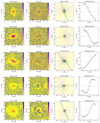 |
Fig. A.1. CL1604 sample of galaxies introduced in Sect. 3 and presented in the same order as in Table A.1. The first and second columns show the original HST-F814W or HSC-z-band images centered on the targets and their residuals after subtracting the 2D model of the galaxies. The pixel scale in the first column corresponds to 0.05″ pix−1 for HST images and 0.2″ pix−1 for HSC images. The third column presents the synthetic velocity field after fitting the simulated rotation curve to the observed curve (assuming the pixel scale of OSIRIS, i.e., 0.25″ pix−1). The solid black parallel lines depict the edges of the slit. The fourth column displays the observed (black dots) and modeled (red line) rotation curve. |
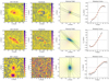 |
Fig. A.1. continued. |
General properties of the Cl1604 galaxy sample.
General properties of the RXJ1347 galaxy sample.
General properties of the XMM2235 galaxy sample.
All Tables
All Figures
|
Fig. 1. Distribution and mean values of the cluster samples according to the main parameters studied in this work: M*, Vmax, and Re. The dashed lines depict the mean values for each parameter and sample. For Abell 901/902, no effective radii are publicly available. |
| In the text | |
|
Fig. 2. Distribution and mean values of the field samples according to the main parameters studied in this work: M*, Vmax, and Re. The dashed lines depict the mean values for each parameter and sample. No effective radii and rotation velocity are publicly available for the samples of Fall & Romanowsky (2018), Posti et al. (2018), and Gillman et al. (2020), while there are no stellar mass values available for Böhm & Ziegler (2016). |
| In the text | |
|
Fig. 3. Star formation activity as a function of stellar mass. Orange, green, and blue stars display cluster galaxies within RXJ1347, CL1604, and XMM2235, respectively. The solid line shows the main sequence of star-forming galaxies at z ∼ 0.45, z ∼ 0.90, z ∼ 1.4 extrapolated by Peng et al. (2010), and the gray area indicates the 3σ scatter. |
| In the text | |
|
Fig. 4. Global environment distribution of galaxies for RXJ1347, CL1604, and XMM2235 clusters. The η value of each object has been computed according to its nearest cluster in Table 1. The dashed line displays the mean value of each sample. |
| In the text | |
|
Fig. 5. Left: B-band TFR. Colored stars represent the different cluster samples that compose our study. The solid black line shows the local B-band TFR (Tully et al. 1998) with a 3σ scatter area reported by Böhm & Ziegler (2016) for galaxies at 0 < z < 1 (gray area). Right: B-band TFR offset evolution. Stars with colored edges represent the distribution of our cluster samples, and their respective mean values are shown as larger circles of the same color. Error bars represent the error of the mean for every sample. Open circles display the Böhm & Ziegler (2016) field sample at 0.1 < z < 1. We binned the field sample into three redshift intervals (0 < z < 0.33, 0.33 < z < 0.66, and 0.66 < z < 1). Black circles depict the mean value and its error for the field sample in every redshift window. The dashed line represents the predicted B-band luminosity evolution by Dutton et al. (2011) in the TFR, and the dash-dotted line at ΔMB = 0 means no size evolution. |
| In the text | |
|
Fig. 6. Symbols and color schemes are the same as in Fig. 5. Left: velocity-size diagram. The solid black line shows the local VSR from Haynes et al. (1999a), with a 3σ scatter gray area around it. Right: velocity-size offset evolution. |
| In the text | |
|
Fig. 7. Specific angular momentum diagram. Orange, green, and blue stars represent the RXJ1347, CL1604, and XMM2235 cluster galaxies, respectively. Black and empty circles show the local universe disk-like samples from Fall & Romanowsky (2018) and Posti et al. (2018), respectively. The small black crosses show the field objects from the KROSS sample at z ∼ 0.9 (Harrison et al. 2017), empty diamonds display the KGES sample at z ∼ 1.5 (Gillman et al. 2020), and the gray squares depict SINS/zC-SINF galaxies at z ∼ 2 (Förster Schreiber et al. 2018). The solid blue line displays the local “Fall relation” for disk galaxies from Fall & Romanowsky (2013). |
| In the text | |
|
Fig. 8. Specific angular momentum offsets (Δlog(j*)) as a function of stellar mass. The solid colored lines depict the mean values and the error of the mean of the mass-binned field samples using bin widths of 0.5 dex. Blue and red lines depict the local universe disk samples from Fall & Romanowsky (2018) and Posti et al. (2018), respectively. The green line shows the distribution of objects from the KROSS sample at z ∼ 0.9 (Harrison et al. 2017). The purple line shows the z ∼ 1.5 KGES sample of galaxies (Gillman et al. 2020), while SINS/zC-SINF galaxies at z ∼ 2 are displayed by the gray line (Förster Schreiber et al. 2018). The dotted lines mark different predicted values of fj as a function of Δlog(j). The light yellow band depicts the predicted scatter in the spin parameter λ assuming fj = 1. The orange, green, and blue circles show the mean Δlog(j)−log(M*) values and their errors for the RXJ1347, CL1604, and XMM2235 cluster galaxies, respectively. Finally, the yellow square displays the average value for Pelliccia et al. (2019) cluster sample. |
| In the text | |
|
Fig. 9. Redshift evolution of j*/M2/3 from z = 0 to z ∼ 2.5. The large black and empty circles show the mean value for the local field galaxies from Fall & Romanowsky (2018) (small black cirles) and Posti et al. (2018) (small empty cirles), respectively. The large empty triangle depicts the average value for the KROSS sample at z ∼ 0.9 (small triangles, Harrison et al. 2017). The empty diamond displays the KGES sample at z ∼ 1.5 (small empty diamonds), and the empty square represents the field galaxies at 2 < z < 2.5 from Förster Schreiber et al. (2018) (small gray squares). The average j*/M2/3 values for the RXJ1347, CL1604, and XMM2235 cluster samples are shown by the orange, green, and blue circles, respectively. The errors of the mean are plotted as error bars for each symbol. The dashed lines represent the expected evolution of the angular momentum with redshift according to the ΛCDM cosmology: j* = M−2/3(z + 1)−n with n = 0.5 (blue) and n = 1 (orange). |
| In the text | |
|
Fig. 10. Left: B-band TFR offsets as a function of the sSFR offsets measured from the main sequence of star-forming galaxies (Peng et al. 2010). The color scheme is the same as in previous figures. Right: B-band offsets with respect to the TFR as a function of global environment (η) for galaxies in our cluster samples. The dashed lines indicate log(η) ≈ 0.3, which is equivalent to the boundary between accreted and infalling galaxies according to Noble et al. (2013). |
| In the text | |
|
Fig. 11. Scale length offsets with respect to the VSR as a function of global environment (η) for galaxies in our cluster samples. The dashed lines indicate log(η) ≈ 0.3, which is equivalent to the boundary between accreted and infalling galaxies, according to Noble et al. (2013). |
| In the text | |
|
Fig. 12. Retained angular momentum fraction (fj) as a function of global environment (η) for galaxies in our cluster samples. The dashed lines indicate log(η) ≈ 0.3, which is equivalent to the boundary between accreted and infalling galaxies, according to Noble et al. (2013). |
| In the text | |
|
Fig. A.1. CL1604 sample of galaxies introduced in Sect. 3 and presented in the same order as in Table A.1. The first and second columns show the original HST-F814W or HSC-z-band images centered on the targets and their residuals after subtracting the 2D model of the galaxies. The pixel scale in the first column corresponds to 0.05″ pix−1 for HST images and 0.2″ pix−1 for HSC images. The third column presents the synthetic velocity field after fitting the simulated rotation curve to the observed curve (assuming the pixel scale of OSIRIS, i.e., 0.25″ pix−1). The solid black parallel lines depict the edges of the slit. The fourth column displays the observed (black dots) and modeled (red line) rotation curve. |
| In the text | |
|
Fig. A.1. continued. |
| In the text | |
Current usage metrics show cumulative count of Article Views (full-text article views including HTML views, PDF and ePub downloads, according to the available data) and Abstracts Views on Vision4Press platform.
Data correspond to usage on the plateform after 2015. The current usage metrics is available 48-96 hours after online publication and is updated daily on week days.
Initial download of the metrics may take a while.