| Issue |
A&A
Volume 646, February 2021
|
|
|---|---|---|
| Article Number | A137 | |
| Number of page(s) | 18 | |
| Section | Interstellar and circumstellar matter | |
| DOI | https://doi.org/10.1051/0004-6361/201935035 | |
| Published online | 19 February 2021 | |
Kinematics and star formation toward W33: a central hub as a hub–filament system
1
National Astronomical Observatories, Chinese Academy of Sciences,
Beijing
100101,
PR China
e-mail: This email address is being protected from spambots. You need JavaScript enabled to view it.
2
CAS Key Laboratory of FAST, National Astronomical Observatories, Chinese Academy of Sciences,
Beijing
100101, PR China
Received:
8
January
2019
Accepted:
17
December
2020
Abstract
Aims. We investigate the gas kinematics and physical properties toward the W33 complex and its surrounding filaments. We study clump formation and star formation in a hub–filament system.
Methods. We performed a large-scale mapping observation toward the W33 complex and its surroundings, covering an area of 1.3° × 1.0°, in 12CO (1–0), 13CO (1–0), and C18O (1–0) lines from the Purple Mountain Observatory (PMO). Infrared archival data were obtained from the Galactic Legacy Infrared Mid-Plane Survey Extraordinaire (GLIMPSE), the Multi-band Imaging Photometer Survey of the Galaxy (MIPSGAL), and the Herschel Infrared Galactic Plane Survey (Hi-GAL). We distinguished the dense clumps from the ATLASGAL survey. We used the GLIMPSE I catalogue to extract young stellar objects.
Results. We found a new hub–filament system ranging from 30 to 38.5 km s−1 located at the W33 complex. Three supercritical filaments are directly converging into the central hub W33. Velocity gradients are detected along the filaments and the accretion rates are in order of 10−3 M⊙ yr−1. The central hub W33 has a total mass of ~1.8 × 10⁵ M⊙, accounting for ~60% of the mass of the hub–filament system. This indicates that the central hub is the mass reservoir of the hub-filament system. Furthermore, 49 ATLASGAL clumps are associated with the hub–filament system. We find 57% of the clumps to be situated in the central hub W33 and clustered at the intersections between the filaments and the W33 complex. Moreover, the distribution of Class I young stellar objects forms a structure resembling the hub–filament system and peaks at where the clumps group; it seems to suggest that the mechanisms of clump formation and star formation in this region are correlated.
Conclusions. Gas flows along the filaments are likely to feed the materials into the intersections and lead to the clustering and formation of the clumps in the hub–filament system W33. The star formation in the intersections between the filaments and the W33 complex might be triggered by the motion of gas converging into the intersections.
Key words: stars: formation / stars: kinematics and dynamics / stars: massive / HII regions / ISM: lines and bands / ISM: molecules
© ESO 2021
1 Introduction
High-mass stars (>8 M⊙) play a vital role in the evolution of interstellar medium (ISM) and their host galaxies. They can enrich the chemical components in the ISM by throwing heavy metal elements into the ISM and therefore promote the chemical evolution of galaxies. However, the formation mechanism of high-mass stars remains unknown. Recently, filaments have found to be prevalent as the main sites of star formation (e.g. Myers 2009; André et al. 2010, 2014; Wang et al. 2015). Particularly in the hub–filament systems, active high-mass star formation is frequently reported in hubs, which host a number of clumps in different phases (e.g. Schneider et al. 2012; Peretto et al. 2013; Hennemann et al. 2014; Friesen et al. 2016; Yuan et al. 2018). In addition, theoretical studies suggest that filaments in the hub–filament systems may act as tributaries, converging mass into the protocluster clumps in the central hub and therefore resulting in vigorous star formation there (Myers 2009; Liu et al. 2012; Gómez & Vázquez-Semadeni 2014). Therefore, identifying and investigating the hub–filament systems can help us to understand the formation of clumps and massive stars.
The W33 complex is a massive star-forming region located at l ~12. °8 and b~−0.2° in the Galactic plane. The parallactic distance of the W33 complex is  (Immer et al. 2013). The W33 complex contains six massive dust clumps (W33 Main, W33A, W33B, W33 Main1, W33A1, and W33B1), which were identified by Immer et al. (2014) using the APEX Telescope Large Area Survey of the Galaxy (ATLASGAL; Schuller et al. 2009). The calculations toward these clumps suggest a total mass of ~ (0.8−8) × 105 M⊙ and an integrated IR luminosity of ~8 × 10⁵ L⊙ (Immer et al. 2014; Kohno et al. 2018). Moreover, molecular line observations toward the W33 complex detect a complex velocity field (e.g. Gardner & Whiteoak 1972; Goldsmith & Mao 1983; Immer et al. 2013; Kohno et al. 2018). As for W33A and W33 Main, emission and absorption peaks were observed at a radial velocity of ~ 35 km s−1, while the spectra toward W33B were seen to peak at ~60 km s−1 (Gardner & Whiteoak 1972; Goldsmith & Mao 1983). Immer et al. (2013) proved that these two velocity components are located at the same parallaxial distance using the water maser emission. Apart from the 35 and 58 km s−1 velocity components associated with the W33 complex, Kohno et al. (2018) detected and identified another velocity component at 45 km s−1, using the CO data from the NANTEN2 and Nobeyama 45 m telescopes. Furthermore, the 21 cm absorption line data suggest that this velocity component is likely partly associated with the W33 complex (Kohno et al. 2018). Kohno et al. (2018) propose that the cloud–cloud collision scenario between the 35 and 58 km s−1 clouds can explain the observed properties.
Visualisation of the W33 complex on a large scale with the three-colour composite of 8, 24, and 70 μm in Fig. 1 suggests that the W33 complex is similar to a central hub surrounded by a set of infrared-dark filaments. In order to highlight the kinematics in the W33 complex and the effects that the surroundings have on the W33 complex, we performed a large-scale CO molecular line observation towards the W33 complex. In addition, the archival infrared data are adopted to probe star formation activities. In Sect. 2, we describe the data sets, and in Sect. 3 the results. We present our analysis and discussions in Sect. 4. Finally, we summarise our main results in Sect. 5.
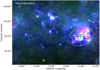 |
Fig. 1 Three-olour composite image towards the W33 complex and its surroundings with blue, green, and red corresponding to Hi-GAL 70 μm (Pilbratt et al. 2010), GLIMPSE 8.0 μm (Benjamin et al. 2003), and MIPSGAL 24 μm (Carey et al. 2009), respectively. The ‘Xs’ symbols represent the massive clumps W33 Main, W33A, W33B, W33 Main1, W33A1, and W33B1 identified by Immer et al. (2014) with the ATLASGAL survey at 870 μm (Schuller et al. 2009). The plus symbols mark the locations of IRDCs identified by Peretto et al. (2016), and the white dashed ellipse represents the W33 complex. |
2 Observations and data reduction
2.1 Purple mountain data
The mapping observations were made towards the W33 complex and its adjacent regions in 12CO (1–0), 13CO (1–0), and C18 O (1–0) lines (the rest frequencies of 115.10, 110.20, and 109.78 GHz) using the PMO 13.7 m radio telescope at De Ling Ha in western China at an altitude of 3200 m during October 2017. The total mapping extent was approximately 80′ × 60′ for all the lines. The half-power beam width (HPBW) at 115 GHz is ~ 53″1. The new nine-beam array receiver system in single-sideband mode (SSB) was used as a front end. Fast Fourier transform spectrometers were used as a back end with a total bandwidth of 1 GHz and 16 384 channels. 12CO (1–0) was observed at upper sideband with a system noise temperature (Tsys) in range of 150−300 K, while 13CO (1–0) and C18O (1–0) were observed simultaneously at lower sideband. The velocity resolution for 12CO (1–0) is ~0.16 km s−1 and for 13CO (1–0)/ C18 O (1–0) is ~0.17 km s−1. The pointing accuracy of the telescope was better than 4″. The phase centreof the observations was (l, b) ~(13. °222, −0. °219) with the position-switch on-the-fly (OTF) mode. The off-position was (l, b) ~(12. °375, −2. °124), devoid of CO emission. The standard chopper wheel calibration technique was used to measure the antenna temperature  corrected for the atmospheric absorption. The final data were recorded in a brightness temperature scale of Tmb (K). The data were reduced and regridded using the software GILDAS (Pety 2005). The pixel sizes of the CO FITS cubes were 30″ × 30″. The 12CO (1–0) data are merely used to estimate the excitation temperatures (see Appendix A), because the velocity components in the 12CO (1–0) spectra cannot be disentangled.
2.2 Archival data sets
2.2.1 Spitzer space telescope
The Galactic Legacy Infrared Mid-Plane Survey Extraordinaire (GLIMPSE) observed the Galactic plane (10° < |l| < 65°, |b| < 1°) with the Infrared Array Camera (IRAC) instrument that can obtain simultaneous broadband images at 3.6, 4.5, 5.8, and 8 μm (Fazio et al. 2004). We downloaded the mid-infrared (MIR) image at 8 μm of this region from the Spitzer GLIMPSE (Benjamin et al. 2003). The archived angular resolutions of IRAC 3.6, 4.5, 5.8, and 8.0 μm are 1.7″, 1.7″, 1.9″, and 2.0″, respectively. In addition, we also extracted the MIPSGAL 24 μm image covering the same region with a resolution of ~6″ (Carey et al. 2009). The point-source catalogue released from the GLIMPSE was used in the following analysis.
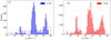 |
Fig. 2 Histograms showing the distributions of the velocity centroid of the C18O (1–0) and 13CO (1–0) fits, respectively. |
2.2.2 ATLASGAL sources
Csengeri et al. (2014) extracted ~10861 compact submillimetre sources with fluxes above 5σ from the maps of the ATLASGAL Survey (Schuller et al. 2009). The ATLASGAL Survey was conducted by the Large APEX Bolometer Camera (LABOCA) at the 12 m diameter APEX telescope at 870 μm (Güsten et al. 2006a,b), dominated by the cold dust emission from dense clumps. It was the first systematic survey of the inner Galactic plane. It has a beam size of ~19.′′2 and in total covers 420 square degrees of the Galactic plane in the Galactic longitude region of − 80° < l < 60°.
3 Results
3.1 Velocity components toward the W33 complex
To fit the spectrum of each pixel in the 13CO (1–0) and the C18O (1–0) fits cubes, we use Behind the Spectrum (BST)2 (Clarke et al. 2018), which is a fully automated routine. A detailed description of BST is given by Clarke et al. (2018). For each component, the BST returns the amplitude (i.e. peak intensity), centroid velocity (υc), velocity dispersion (σc), and the reduced  values of each spectrum. For accuracy, we check all the fits, and manually remake the Gaussian fits to each spectrum. If it is fitted not well, we will exclude it. And the returned amplitudes have to be over 1 K (5σ) for C18O (1–0) and 3 K (6σ) for 13CO (1–0). The velocity dispersions σc have to be more than 0.51 km s−1 (3 channels). Moreover any two fits from the same spectrum have a υc separation greater than 0.51 km s−1. Figure 2 shows the returned υc histograms of the C18O (1–0) and 13CO (1–0) fits, respectively. From the υc distributions, we identify six velocity components along the line of sight toward the W33 complex. These are in the ranges of 2–15 km s−1, 15–21 km s−1, 21–28 km s−1, 30–44 km s−1, 44–48 km s−1, and 48–60 km s−1, marked with the black dashed boxes in Fig. 2. In addition, we estimate the excitation temperatures and the optical depths for the fits of two lines via Eqs. (A.1) and (A.2). The H2 column densities for the C18O fits are also calculated using Eq. (A.3). The distribution diagrams of these parameters are shown in Figs. A.1–A.5. From the figures, we can see that the 13CO lines are really optically thick in the dense regions with N(H2) ≳ 1023 cm−2. Here, we use the optically thin C18O (1–0) line to determine which velocity component is associated with the W33 complex.
Based on the above six velocity ranges, we make the C18 O (1–0) integrated intensity maps overlaid on the Spitzer 8 μm emission, as shown in Fig. 3. The C18O (1–0) emission reveals completely different structures for the six velocity components. Also, from the morphologies of the C18 O (1–0) emission, we find that the velocity components of 30–44 km s−1 and 48–60 km s−1 seem associated with the W33 complex and W33B, respectively. This result is consistent with those of Immer et al. (2013) and Kohno et al. (2018). On a larger scale, our CO velocity components reveal a number of other structures besides the W33 complex. In particular, the 30–44 km s−1 velocity component in Fig. 3d is closely associated with a set of infrared dark filaments, referred to here as f1-f5, which seem to surround the W33 complex. Below, we further use the position-position-velocity (PPV) cubes to discern the velocity structures associated with the W33 complex in the 30–44 km s−1 range.
3.2 The hub–filament system
3.2.1 A new hub–filament system identified toward the W33 complex
To highlight the velocity structures in 30–44 km s−1, we make theC18O (1–0) PPV space using the BST obtained fits cube, as shown in Fig. 4. According to the values of the centroid velocities υc, we mark the colour for each point. Meanwhile, the 3D projections of all the points are plotted on each of the axes. On each projection plane in Fig. 4, we identified three small velocity ranges, namely 30–38.5 km s−1, 38.5–42 km s−1, and 42–44 km s−1. Figure 5 shows the centroid velocity distribution diagrams for the above three velocity ranges. From Fig. 5, we find that the C18O (1–0) emission presents different structures in the three ranges. The structure of the 38.5–42 km s−1 velocity component in Fig. 5b mainly presents an east-to-west large-scale filament containing filaments f4 and f5. From Fig. 5c, we see that the velocity component of 42–44 km s−1 is mainly coincident with some isolated structures. While the velocity component of 30–38.5 km s−1 is closely associated with the W33 complex and filaments f1-f3; below we focus on this component. In Fig. 5a, an ellipse represents the W33 complex. To avoid confusion, we rename the filaments adjacent to the W33 complex as hf1, hf2, and hf3. The three filaments traced by the black lines gather in the direction of the W33 complex. Similar to the structure of NGC 2264 (Kumar et al. 2020), the 30–38.5 km s−1 velocitycomponent appears to show a hub–filament system, whose central hub is the W33 complex.
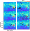 |
Fig. 3 Panels a–f: velocity-integrated C18O (1–0) contours in the velocity ranges of 2–15 km s−1, 15–21 km s−1, 21–28 km s−1, 30–44 km s−1, 44–48 km s−1, and 48–60 km s−1 respectively, overlaid on the Spitzer 8 μm image. The white dashed lines in (d) show the filaments detected in 30–44 km s−1, and the magenta dashed lines in (e) represent the cutting directions of Fig. 10. The colour bar represents the flux at 8 μm in units of Myr sr−1. |
3.2.2 Physical properties of the hub–filament system
Furthermore, we estimate the physical parameters of the hub–filament system, which are all listed in Table 1. From Col. 12 of Table 1, we see that the central hub W33 has an equivalent radius of 6.0 pc. The filament hf2is the longest with a length up to 15.7 pc, while hf1 is the shortest with a length of 7.5 pc. The widths of the filaments hf1, hf2, and hf3 are 4.6, 3.8, and 3.0 pc, respectively. Considering the sensitivity limits of C18 O (1–0) (Amplitude > 5σ) as well as the inclinations, the measured lengths and widths of the filaments should be a lower limit. Column 4 of Table 1 presents the velocity ranges spanned by these structures. The minimum velocity interval is ~ 5 km s−1 in the filament hf3, further demonstrating the complicated velocity structures in the whole hub–filament system. In addition, Col. 7 in Table 1 shows the minimum ratios of the non-thermal velocity dispersions to the sound speeds (σNT∕cs) in these structures. We can see that all the ratios σNT∕cs are greater than 1, suggesting that the whole hub–filament system is supersonic, probably dominated by the turbulence (Liu et al. 2018). The hub–filament system has a mean excitation temperature of ~ 17.5 K, less than that of the W33 complex (~20.7 K), indicating that the central hub is warmer than its surrounding environment. Also, from Cols. 8-9 of Table 1, both the central hub W33 and the filaments hf1, hf2, and hf3 have a mean H2 column density in magnitude of 1022 cm−2 and a mean H2 number density on the orderof 104 cm−3. In addition, the W33 complex has a total mass of 1.8 × 10⁵ M⊙, which is consistent with previous findings (e.g. Immer et al. 2014) and accounts for 60% of the mass of the hub–filament system. The masses of the filaments hf1, hf2, and hf3 are in the range of (2.6−4.7) × 104 M⊙. These three filaments account for ~35% of the mass of the hub–filament system, illustrating that the mass of the hub–filament system is mainly concentrated in the central hub W33.
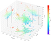 |
Fig. 4 C18O (1–0) PPV space in the velocity interval of 30–44 km s−1. The projections on the three axes are presented. The colour of each point represents the centroid velocity at that point, corresponding to the colour bar shown to the right of the panel. The symbols ‘Xs’ are similar to those in Fig. 1, and the W33 complex is marked by the black dashed lines or the dashed ellipses on the three projections. |
Main properties of the filaments and the W33 complex in the hub-filament system.
3.3 ATLASGAL 870 μm clumps in the hub–filament system
The ATLASGAL 870 μm emission traces the distribution of cold dust (Beuther et al. 2012). From the catalogue of the ATLASGAL 870 μm clumps (Urquhart et al. 2018), we extract 49 clumps associated with the hub–filament system based on their VLSR and distances. The physical parameters of these 49 clumps are presented in Table 2. All the clumps are found at a distance of 2.6 kpc, which is consistent with the parallax distance of  (Immer et al. 2013). In addition, the distribution of the clumps with the same distance in the hub–filament system provides further evidence that the W33 complex and the surrounding filaments constitute a complete system. Also, their VLSR are in the range of 32.7−38.4 km s−1. We overlay the clumps on the C18O (1–0) centroid velocity distribution map in Fig. 5a, which reveals that 28 of them are located in the central hub W33. The other clumps are mainly distributed along the spines of the filaments hf3 (10) and hf2 (6). We also made histograms of radius, dust temperature, mass, and H2 column density of the clumps in the W33 complex and in the filaments; see Fig. 6. We find that the clumps are warmer and denser with larger sizes in the W33 complex, while the mean values of the mass are the same for the clumps in the W33 complex and in the filament.
Furthermore, Urquhart et al. (2018) classified ~8000 ATLASGAL870 μm clumps into four evolutionarysequences: quiescent (70 μm weak), protostellar (MIR-dark but FIR-bright), young stellar objects (YSOs; MIR-bright), and MSF (associated with massive star formation tracers, such as radio-bright HII regions and methanol masers). From Col. 13 of Table 2, we see that the extracted 49 clumps consist of 12 (~ 24%) quiescent clumps, 14 (~ 29%) protostellar clumps, 20 YSO (~41%) clumps, and 3 MSF clumps (~6%). It appears that more than 76% of the clumps are probably forming stars, indicating that the hub–filament system provides a good environment for star formation. In addition, Table 3 presents the percentages of each stage in the central hub W33 and in the filaments. Firstly, we find that only the central hub W33 contains three MSF clumps. We also find that 70% of the YSO clumps are in the central hub W33, while ~64% of the protostellar clumps are in the filaments. The percentages of the quiescent clumps are equal in the central hub and the filaments.
To investigate the capability of the clumps in the hub–filament system to form massive stars, we consider the relationship between mass and size, as shown in Fig. 7. The yellow shaded region represents a parameterspace devoid of massive star formation, as determined by Kauffmann & Pillai (2010), of  . From Fig. 7, we find that ~46% of the clumps in the central hub W33 and ~57% of the clumps in the filaments lie above the threshold, suggesting significant potential to form massive stars. Therefore, the hub–filament system is likely to be a suitable environment to form massive stars.
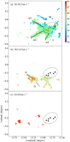 |
Fig. 5 Velocity distributions in 30–38.5 km s−1 (panel a), 38.5–42 km s−1 (panel b), and 42–44 km s−1 (panel c), respectively. The points are coloured with the velocity values shown in the right colour bar. The asterisks represent the MSF clumps, ‘▽’ mark the YSO clumps, ‘△’ flag the protostellar clumps, and the squares are for the quiescent clumps. The black lines denote the spines of the filaments hf1, hf2, and hf3. The clumps are coded with different colours in the W33 complex (yellow) and in the filaments (red), respectively. |
3.4 Distribution of young stellar objects toward the hub–filament system
To study the star formation activity in the hub–filament system, we search for YSOs using the GLIMPSE ISpring’07 catalogue. In total, 47 787 near-infrared (NIR) sources with 3.6, 4.5, 5.8, and 8.0 μm are selected in the observation zoom. The IRAC [5.8]-[8.0] versus [3.6]-[4.5] colour–colour (CC) diagram is a useful tool for identifying YSOs with infrared excess (Allen et al. 2004). Based on the criteria of Allen et al. (2004), these NIR sources are classified into three evolutionary stages, as shown in Fig. 8. Here, 811 NIR sources are identified as Class I sources, which are protostars with circumstellar envelopes and have an age of ~ 105 yr, and 1252 sources are Class II sources, which are disc-dominated objects with an age of ~ 106 yr. The remaining NIR sources are other sources (such as classical T Tauri, Herbig Ae/Be). Here, Class I and Class II sources are selected as the YSOs.
As the identified Class II YSOs are almost uniformly distributed in the hub–filament system, we only show the distribution of all the identified Class I sources overlaid on the C18 O (1–0) emission map in Fig. 9a. We note that Class I sources are preferentially situated in the regions where clumps are clustered in the hub–filament system. The clustering of YSOs in a given area can help us identify the active star-forming regions. To highlight the clustering behaviour of YSOs within the hub–filament system, we analysed the surface density distribution of the identified Class I YSOs in Fig. 9b. The lowest level of the contours is ~0.5 pc−2 to get rid of the effect of the foreground and background objects. In Fig. 9b, we find that the surface density distribution of the Class I YSOs resembles the structure of the hub–filament system. Moreover, the peaks of the Class I YSO density distribution are located where the clumps group, which appears to suggest that the mechanism of clump and YSO formation inthe hub–filament system might be the same.
Summary of the parameters for the 49 ATLASGAL clumps in the hub-filament system.
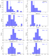 |
Fig. 6 Comparisons of the clump physical parameter distributions in the central hub W33 and in the filaments. |
Percentages of the clumps in each stage in different places.
4 Discussion
In order to explore the clump and YSO formation in the hub–filament system, we need to analyse the stability of the central hub W33, which can be calculated using the expression  , where R is the equivalent radius of the central hub W33, and
  , the mean velocity dispersion. The derived αvir from the optically thin C18O (1–0) line is ~0.04. When αvir is less than 1, the central hub W33 is likely gravitationally bound and perhaps collapsing. At the same time, for the filaments hf1, hf2, and hf3, the difference between the critical mass to length ratio
  and the linear mass M∕L can tell us the stability of the filaments (Jackson et al. 2010). When
  , the filaments are dominated by gravity and may be collapsing. The
  can be derived from
  , which is mainly caused by turbulence (Jackson et al. 2010), and the M∕L are calculated using the total masses M and lengths L of the filaments hf1, hf2, and hf3. The derived M∕L are the upper limits due to inclination and projection effects. Our computed results are listed in Cols. 14–15 of Table 1. They indicate that filaments hf1, hf2, and hf3 are probably collapsing globally.
Figure 10 shows the difference between the velocities of the filaments and the junctions as a function of distance to junction. The points in Fig. 10 are extracted along the spine of each filament. From Fig. 10, we can see that the filament hf1 shows a transition on the tail within the last 2 pc, but this might be inaccurate because of possible confusion with other clouds. Indeed, we detect a ~ 39 km s−1 filament there (see Sect. 3.2.1 and Fig. 5b). If ignoring the decreasing trend of hf1, the filaments hf1, hf2, and hf3 all present monotonically increasing profiles. The resultant velocity gradients are consistent with the ones reported in other collapsing filaments (Peretto et al. 2014; Liu et al. 2016; Yuan et al. 2018). The velocity gradients for these filaments are estimated to be 0.32, 0.11, and 0.10 km s−1 pc−1, respectively.The values are comparable to those detected in previous studies (Peretto et al. 2014; Yuan et al. 2018).
Both cloud rotation and accretion flows along the filament can result in this kind of velocity gradient (Veena et al. 2018). To examine therotational feature in the hub–filament system, we constructed position–velocity (PV) diagrams of C18 O (1–0) along the cuttings in Fig. 3e, as shown in Fig. 11. The white dashed lines mark the location of the W33 complex. The PV plots in Fig. 11 reveal the velocity gradients between the filaments and the W33 complex as well as along the filaments, but no signs of a Keplerian rotation signature are observed. Therefore, we propose that the hub–filament system is not rotating.
On the other hand, accretion flow along the filament could also be causing the smoothed velocity gradient (Kirk et al. 2013, and reference therein). Following Kirk et al. (2013), we derived the gas accretion rate Ṁ for a simple cylindrical cloud,
 (1)
(1)
in which α is assumed as an inclination angle of 45° without considering the projection effect (Yuan et al. 2018; Veena et al. 2018). The accretion rates of the filaments are calculated as 8.5 × 10⁻³, 5.3 × 10⁻³, and 3.2 × 10⁻³ M⊙ yr−1 for the filaments hf1, hf2, and hf3, respectively, while residual effects from the velocity coherence widely detected in Giant Molecular Filaments (GMFs) cannot be ruled out (Ragan et al. 2014; Wang et al. 2015). From Fig. 5a, we propose that the central hub W33 is probably being fed by the filaments hf1, hf2, and hf3 directly. The total accretion rate is ~ 1.7 × 10⁻² M⊙ yr−1, two orders of magnitude greater than rates found by other studies (Yuan et al. 2018; Chen et al. 2019; Treviño-Morales et al. 2019). Given that our velocity gradients are comparable to those in other studies (Yuan et al. 2018; Chen et al. 2019; Treviño-Morales et al. 2019), this larger accretion rate could be caused by the two orders of magnitude greater masses of the filaments hf1, hf2, and hf3. Furthermore, this higher accretion rate on the larger scale probably leads to the much larger mass in the W33 complex and probably promotes proto-cluster formation in the W33 complex (Messineo et al. 2015). Consequently, the W33 complex is possibly accumulating about 1.7 × 10⁴ M⊙ Myr−1 as an upper limit.
The central hub W33 has a total mass of ~1.8 × 10⁵ M⊙, accounting for ~60% of the mass of the hub–filament system. This indicates that the central hub is the mass reservoir of the hub–filament system. The clumps in Fig. 5a are clustered in the intersection between filaments hf1, hf2, and hf3 and the central hub W33, indicating that gas flows along the filaments are probably channelling mass to the junction and promoting clump formation in the intersection. Moreover, the other clumps are distributed in the filaments and the W33 complex might be the result of global collapse. Global collapse could be causing the accretion of materials radially into the central zones, providing mass for clump formation.
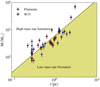 |
Fig. 7 Mass–size relationship of the clumps with masses determined. The yellow shaded region represents the parameter space devoid of massive star formation, where
|
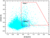 |
Fig. 8 IRAC colour–colour plot for the sources in our observational region. The regions indicated the stellar evolutionary stage as defined by Allen et al. (2004). Class I sources represent protostars with circumstellar envelopes and Class II are disc-dominated objects. |
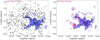 |
Fig. 9 Panel a: Class I YSOs marked by plus symbols overlaid on the C18O (1–0) emission. Panel b: corresponding overlay of Class I YSOs surface density contours on the C18 O (1–0) emission. The contour levels start from 0.5 to 1.7 pc−2 (magenta contours) in steps of 0.13 pc−2. The different symbols represent the clumps in different stages, similar to those in Fig. 5a. In addition, the clumps marked with the red colour are in the velocity range of 38.5–42 km s−1. |
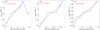 |
Fig. 10 Line-of-sight velocity difference of C18O (1–0) as a function of position from junctions. |
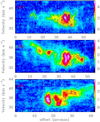 |
Fig. 11 Position–velocity diagrams of C18O (1–0) along the cuts in Fig. 3e. The contour levels start from 5σ to the peak integrated intensity by 3σ (σ = 0.2 K). The vertical white dashed lines mark the location of the W33 complex, and the filaments detected are labelled in each panel. |
5 Summary and conclusions
We present the large-scale molecular 12CO (1–0), 13CO (1–0), and C18O (1–0) lines, and infrared observations toward the W33 complex and its surroundings. Our main findings are summarised as follows:
- 1.
According to the centroid velocity distributions of the Gaussian fits to all the 13CO (1–0) and C18O (1–0) lines, six velocity components are distinguished along the line of sight toward the W33 complex from 0 to 70 km s−1, namely 2–15 km s−1, 15–21 km s−1, 21–28 km s−1, 30–44 km s−1, 44–48 km s−1, and 48–60 km s−1. The velocity component 30–44 km s−1 on large scale is likely to be associated with the W33 complex from the CO emission in Fig. 3d.
- 2.
The PPV space of C18O (1–0) revealsthat the 30–44 km s−1 velocity component consists of three different velocity components in 30–38.5 km s−1, 38.5–42 km s−1, and 42–44 km s−1. The 30–38.5 km s−1 velocity component shows a real hub–filament system, whose central hub is the W33 complex. Three filaments hf1, hf2, and hf3 are spatially adjacent to the W33 complex in different directions.
- 3.
The central hub W33 has a mass of 1.8 × 10⁵ M⊙, accounting for about 60% of the mass of the hub–filament system, and the masses of the filaments hf1, hf2, and hf3 are in the range of (2.6−4.7) × 104 M⊙. The mass of the hub–filament system is concentrated in the W33 complex and the adjacent filaments (~ 95%). The central hub W33 is globally collapsing, as suggsted by the virial parameter αvir which is lower than 1. The filaments hf1, hf2, and hf3 are supercritical with mass per unit length ranging from 2214 to 3467 M⊙ pc−1, indicating that they are also globally collapsing. Regular velocity gradients along the filaments hf1, hf2, and hf3 suggest that these filaments are channelling materials into the junctions with an accretion rate of ~ 1.7 × 10⁻² M⊙ yr−1.
- 4.
In total, 49 dense clumps are identified to be associated with the hub–filament system, and over 57% of the clumps (28) are located at the central hub W33, including 3 MSF clumps. The other clumps are situated in the filaments without the MSF clumps. Also, 70% of the YSO clumps of the system are found in the central hub. We find that ~ 46% of the clumps in the central hub W33 and ~57% of the clumps in the filaments lie above the mass threshold permitting massive star formation, suggesting significant potential to form massive stars in those regions.
- 5.
The surface density distribution of Class I YSOs in this system shows a similar structure to the hub–filament system, and the peaks in this distribution are at the junctions between the filaments and the W33 complex, where there are concentrations of clumps. Gas flows along the filaments possibly provide the mass for clump formation and probably create the star formation in the intersections.
Based on the above findings, we conclude that the W33 complex is likely to be a central hub of a hub–filament system. Also, the gas flows along the tributary filaments in the system probably promote the proto-cluster formation in the W33 complex.
Acknowledgements
We are grateful to the staff at the Qinghai Station of PMO for their assistance during the observations. Thanks for the Key Laboratory for Radio Astronomy, CAS, for partly supporting the telescope operation. This work is partly supported by the National Natural Science Foundation of China 11703040 and the National Natural Science Foundation of China 11933011. This work has made used of data from the NASA/IPAC Infrared Science Archive, which is operated by the Jet Propulsion Laboratory, California Institute of Technology, under contract with the National Aeronautics and Space Administration. The ATLASGAL project is a collaboration between the Max-Planck-Gesellschaft, the European Southern Observatory (ESO) and the Universidad de Chile. It includes projects E-181.C-0885, E-078.F-9040(A), M-079.C-9501(A), M-081.C-9501(A) plus Chilean data. C.-P.Z. acknowledges supports from the NAOC Nebula Talents Program, and the Cultivation Project for FAST Scientific Payoff and Research Achievement of CAMS-CAS.
Appendix A Calculations to derive the physical parameters of each fit
In general, the 12CO (1–0) emission is optically thick. Therefore, we can estimate the excitation temperature Tex for each fit of 13CO (1–0) and C18O (1–0) respectively via the flowing formula (Garden91 et al. 1991; Pineda et al. 2008)
![Mathematical equation: \begin{equation*}T_{\textrm{ex}}\,{=}\,\frac{5.53}{\textrm{ln}[1+5.53/(T_{\textrm{mb}}(^{12}\textrm{CO})+0.82)]}, \end{equation*}](/articles/aa/full_html/2021/02/aa35035-19/aa35035-19-eq13.png) (A.1)
(A.1)
where  is the 12CO (1–0) peak intensity in the velocity range (υc − 1.175σc, υc + 1.175σc) of each fit from the 13CO (1–0) and C18 O (1–0) spectra, respectively. Because we check and correct every Gaussian fit from the BST code, the median errors for the peak intensity, the centroid velocity υc, and the velocity dispersions σc are about 1%. Therefore, the derived median excitation temperatures for the 13CO (1–0) fits and C18 O (1–0) fits are about 1.7%.
Therefore, we can derive the non-thermal velocity dispersion σNT and the ratio of σNT to the sound speed cs. The non-thermal velocity dispersion σNT of each fit is calculated using the following equation:  , where σc is the dispersion of each fit, kB is the Boltzmann constant, Tk is the kinetic temperature (here Tk ≈ Tex under the assumption of local thermodynamic equilibrium LTE; Morgan et al. 2010), mgas is the mass of the molecule, and the sound speed cs can be obtained as
  , in which mH is the mass of a hydrogen atom and
  is the mean molecular weight per hydrogen molecule (Kauffmann et al. 2008). Thereby, the median errors of σNT and σNT∕cs are ~ 1.1% and ~ 1.4%, resulting from the errors of the excitation temperature and the velocity dispersion.
Furthermore, assuming the same excitation temperature between the 12CO (1–0) line and the C18 O (1–0) lines, we can estimate theoptical depth τ of the C18O (1–0) lines, the H2 column density, the H2 number density, and the mass of each fit. The optical depth τ of the C18O (1–0) lines can be derived from the equation as follows (Garden91 et al. 1991; Pineda et al. 2008):
![Mathematical equation: \begin{equation*}\tau\,{=}\,{\rm-ln}\left[1-\frac{T_{\textrm{mb}}}{T_0(J(T_{\textrm{ex}})-J(T_{\textrm{bg}}))}\right], \end{equation*}](/articles/aa/full_html/2021/02/aa35035-19/aa35035-19-eq18.png) (A.2)
(A.2)
where Tmb is the amplitude (i.e. peak intensity) of each fit, T0 = hν∕k, h is the Planck constant, k is the Boltzmann constant, and ν is the transition frequency of the optically thin line. Also, J(T) is defined by J(T) = 1∕(exp(T0∕T) − 1). The median uncertainty of the optical depth is about 3%, caused by the errors of the excitation temperature and the peak intensity.
We can then determine the column density of the optically thin molecular line under the assumption of LTE via the expression (Sanhueza et al. 2012):
 (A.3)
(A.3)
where B is the rotational constant of the molecule, J is rotational quantum number of the lower state,  is the permanent dipole moment of the molecule, Tbg = 2.73 is the background temperature, and Eu is the energy of the upper level. The values of these can be obtained from the Cologne Database for Molecular Spectroscopy3 (CDMS; Müller et al. 2001, 2005). Also, W is the integrated intensity, which can be estimated using FWHW × amplitude. Next, the H2 column density of each component can be calculated by N(H2)∕N(C18O) ≈ 6 × 10⁶ for dense regions (Frerking et al. 1982). The median uncertainty of the H2 column density is estimated to be 2% using the median errors of the excitation temperature, the optical depth, the centroid velocity, the velocity dispersion, and the peak intensity. The H2 number density and the mass have the same uncertainties as the H2 column density with a median value of 2%.
Finally, we calculate the H2 number density and mass of each component by assuming the point as a rectangle shape. The equations are as follows:
 (A.4)
(A.4)
 (A.5)
(A.5)
where Rpixel is the size of a pixel,  is the mean molecular weight per hydrogen molecule, and mH is the mass of a hydrogen atom.
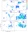 |
Fig. A.1 Distributions of the optical depth of the 13CO (1–0) line in different velocity components. The velocity interval of each panel is shown in the left-top corner. The dashed ellipse in each panel marks the W33 complex (Immer et al. 2014; Kohno et al. 2018) and the ‘Xs’ symbols are the same as those in Fig. 1. |
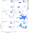 |
Fig. A.2 Distributions of the optical depth of the C18O (1–0) line in different velocity components. The velocity interval of each panel is shown in the left-top corner. The dashed ellipse in each panel marks the W33 complex (Immer et al. 2014; Kohno et al. 2018) and the ‘Xs’ symbols are the same as those in Fig. 1. |
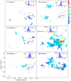 |
Fig. A.3 Distributions of the excitation temperature in different velocity components. The velocity interval of each panel is shown in the left-top corner. The dashed ellipse in each panel marks the W33 complex (Immer et al. 2014; Kohno et al. 2018)and the ‘Xs’ symbols are the same as those in Fig. 1. The colour bar is in units of K. |
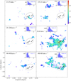 |
Fig. A.4 Distributions of the C18O (1–0) velocity dispersion in different velocity components. The velocity interval of each panel is shown in the left-top corner. The dashed ellipse in each panel marks the W33 complex (Immer et al. 2014; Kohno et al. 2018) and the ‘Xs’ symbols are the same as those in Fig. 1. The colour bar is in units of km s−1. |
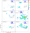 |
Fig. A.5 Distributions of the H2 column density in different velocity components. The velocity interval of each panel is shown in the left-top corner. The dashed ellipse in each panel marks the W33 complex (Immer et al. 2014; Kohno et al. 2018) and the ‘Xs’ symbols are the same as those in Fig. 1. The colour bar is logarithmic with units of cm−2. |
References
- Allen, L. E., Calvet, N., D’Alessio, P., et al. 2004, ApJS, 154, 363 [NASA ADS] [CrossRef] [Google Scholar]
- André, P., Men’shchikov, A., Bontemps, S., et al. 2010, A&A, 518, L102 [NASA ADS] [CrossRef] [EDP Sciences] [Google Scholar]
- André, P., Di Francesco, J., Ward-Thompson, D., et al. 2014, Protostars and Planets VI, eds. H. Beuther, R. S. Klessen, C. P. Dullemond, & T. Henning (Tucson, AZ: University of Arizona Press), 27 [Google Scholar]
- Benjamin, R. A., Churchwell, E., Babler, B. L., et al. 2003, PASP, 115, 953 [NASA ADS] [CrossRef] [Google Scholar]
- Beuther, H., Tackenberg, J., Linz, H., et al. 2012, ApJ, 747, 43 [NASA ADS] [CrossRef] [Google Scholar]
- Carey, S. J., Noriega-Crespo, A., Mizuno, D. R., et al. 2009, PASP, 121, 76 [NASA ADS] [CrossRef] [Google Scholar]
- Chen, H.-R. V., Zhang, Q., Wright, M. C. H., et al. 2019, ApJ, 875, 24 [NASA ADS] [CrossRef] [Google Scholar]
- Clarke, S. D., Whitworth, A. P., Spowage, R. L., et al. 2018, MNRAS, 479, 1722 [NASA ADS] [CrossRef] [Google Scholar]
- Csengeri, T., Urquhart, J. S., Schuller, F., et al. 2014, A&A, 565, A75 [NASA ADS] [CrossRef] [EDP Sciences] [Google Scholar]
- Fazio, G. G., Hora, J. L., Allen, L. E., et al. 2004, ApJS, 154, 10 [NASA ADS] [CrossRef] [Google Scholar]
- Frerking, M. A., Langer, W. D., & Wilson, R. W. 1982, ApJ, 262, 590 [NASA ADS] [CrossRef] [Google Scholar]
- Friesen, R. K., Bourke, T. L., Di Francesco, J., Gutermuth, R., & Myers, P. C. 2016, ApJ, 833, 204 [NASA ADS] [CrossRef] [Google Scholar]
- Garden91, R. P., Hayashi, M., Gatley, I., Hasegawa, T., & Kaifu, N. 1991, ApJ, 374, 540 [NASA ADS] [CrossRef] [Google Scholar]
- Gardner, F. F., & Whiteoak, J. B. 1972, ApJ, 12, L107 [Google Scholar]
- Goldsmith, P. F., & Mao, X. J. 1983, ApJ, 265, 791 [NASA ADS] [CrossRef] [Google Scholar]
- Gómez, G. C., & Vázquez-Semadeni, E. 2014, ApJ, 791, 124 [NASA ADS] [CrossRef] [Google Scholar]
- Güsten, R., Booth, R. S., Cesarsky, C., et al. 2006a, SPIE Conf. Ser., 6267, 626714 [Google Scholar]
- Güsten, R., Nyman, L. Å., Schilke, P., et al. 2006b, A&A, 454, L13 [NASA ADS] [CrossRef] [EDP Sciences] [Google Scholar]
- Guzmán, A. E., Sanhueza, P., Contreras, Y., et al. 2015, ApJ, 815, 130 [NASA ADS] [CrossRef] [Google Scholar]
- Hennemann, M., Motte, F., & Schneider, N. 2014, The Labyrinth of Star Formation (Cham: Springer), 36, 271 [Google Scholar]
- Immer, K., Reid, M. J., Menten, K. M., Brunthaler, A., & Dame, T. M. 2013, A&A, 553, A117 [NASA ADS] [CrossRef] [EDP Sciences] [Google Scholar]
- Immer, K., Galván-Madrid, R., König, C., Liu, H. B., & Menten, K. M. 2014, A&A, 572, A63 [NASA ADS] [CrossRef] [EDP Sciences] [Google Scholar]
- Jackson, J. M., Finn, S. C., Chambers, E. T., Rathborne, J. M., & Simon, R. 2010, ApJ, 719, L185 [NASA ADS] [CrossRef] [Google Scholar]
- Kauffmann, J., & Pillai, T. 2010, ApJ, 723, L7 [NASA ADS] [CrossRef] [Google Scholar]
- Kauffmann, J., Bertoldi, F., Bourke, T. L., Evans, N. J., I., & Lee, C. W. 2008, A&A, 487, 993 [NASA ADS] [CrossRef] [EDP Sciences] [Google Scholar]
- Kirk, H., Myers, P. C., Bourke, T. L., et al. 2013, ApJ, 766, 115 [NASA ADS] [CrossRef] [Google Scholar]
- Kohno, M., Torii, K., Tachihara, K., et al. 2018, PASJ, 70, S50 [Google Scholar]
- Kumar, M. S. N., Palmeirim, P., Arzoumanian, D., & Inutsuka, S. I. 2020, A&A, 642, A87 [EDP Sciences] [Google Scholar]
- Liu, H. B., Hsieh, P.-Y., Ho, P. T. P., et al. 2012, ApJ, 756, 195 [NASA ADS] [CrossRef] [Google Scholar]
- Liu, T., Zhang, Q., Kim, K.-T., et al. 2016, ApJ, 824, 31 [NASA ADS] [CrossRef] [Google Scholar]
- Liu, X.-L., Xu, J.-L., Ning, C.-C., Zhang, C.-P., & Liu, X.-T. 2018, Res. A&A, 18, 004 [Google Scholar]
- Messineo, M., Clark, J. S., Figer, D. F., et al. 2015, ApJ, 805, 110 [NASA ADS] [CrossRef] [Google Scholar]
- Morgan, L. K., Figura, C. C., Urquhart, J. S., & Thompson, M. A. 2010, MNRAS, 408, 157 [NASA ADS] [CrossRef] [Google Scholar]
- Müller, H. S. P., Thorwirth, S., Roth, D. A., & Winnewisser, G. 2001, A&A, 370, L49 [NASA ADS] [CrossRef] [EDP Sciences] [Google Scholar]
- Müller, H. S. P., Schlöder, F., Stutzki, J., & Winnewisser, G. 2005, J. Mol. Struct., 742, 215 [Google Scholar]
- Myers, P. C. 2009, ApJ, 700, 1609 [NASA ADS] [CrossRef] [EDP Sciences] [Google Scholar]
- Peretto, N., Fuller, G. A., Duarte-Cabral, A., et al. 2013, A&A, 555, A112 [NASA ADS] [CrossRef] [EDP Sciences] [Google Scholar]
- Peretto, N., Fuller, G. A., André, P., et al. 2014, A&A, 561, A83 [NASA ADS] [CrossRef] [EDP Sciences] [Google Scholar]
- Peretto, N., Lenfestey, C., Fuller, G. A., et al. 2016, A&A, 590, A72 [NASA ADS] [CrossRef] [EDP Sciences] [Google Scholar]
- Pety, J. 2005, SF2A-2005: Semaine de l’ Astrophysique Francaise, eds. F. Casoli, T. Contini, J. M. Hameury, & L. Pagani, 721 [Google Scholar]
- Pilbratt, G. L., Riedinger, J. R., Passvogel, T., et al. 2010, A&A, 518, L1 [CrossRef] [EDP Sciences] [Google Scholar]
- Pineda, J. E., Caselli, P., & Goodman, A. A. 2008, ApJ, 679, 481 [Google Scholar]
- Ragan, S. E., Henning, T., Tackenberg, J., et al. 2014, A&A, 568, A73 [NASA ADS] [CrossRef] [EDP Sciences] [Google Scholar]
- Sanhueza, P., Jackson, J. M., Foster, J. B., et al. 2012, ApJ, 756, 60 [NASA ADS] [CrossRef] [Google Scholar]
- Schneider, N., Csengeri, T., Hennemann, M., et al. 2012, A&A, 540, L11 [NASA ADS] [CrossRef] [EDP Sciences] [Google Scholar]
- Schuller, F., Menten, K. M., Contreras, Y., et al. 2009, A&A, 504, 415 [NASA ADS] [CrossRef] [EDP Sciences] [Google Scholar]
- Treviño-Morales, S. P., Fuente, A., Sánchez-Monge, Á., et al. 2019, A&A, 629, A81 [NASA ADS] [CrossRef] [EDP Sciences] [Google Scholar]
- Urquhart, J. S., König, C., Giannetti, A., et al. 2018, MNRAS, 473, 1059 [NASA ADS] [CrossRef] [Google Scholar]
- Veena, V. S., Vig, S., Mookerjea, B., et al. 2018, ApJ, 852, 93 [NASA ADS] [CrossRef] [Google Scholar]
- Wang, K., Testi, L., Ginsburg, A., et al. 2015, MNRAS, 450, 4043 [NASA ADS] [CrossRef] [MathSciNet] [Google Scholar]
- Yuan, J., Li, J.-Z., Wu, Y., et al. 2018, ApJ, 852, 12 [NASA ADS] [CrossRef] [Google Scholar]
All Tables
All Figures
|
Fig. 1 Three-olour composite image towards the W33 complex and its surroundings with blue, green, and red corresponding to Hi-GAL 70 μm (Pilbratt et al. 2010), GLIMPSE 8.0 μm (Benjamin et al. 2003), and MIPSGAL 24 μm (Carey et al. 2009), respectively. The ‘Xs’ symbols represent the massive clumps W33 Main, W33A, W33B, W33 Main1, W33A1, and W33B1 identified by Immer et al. (2014) with the ATLASGAL survey at 870 μm (Schuller et al. 2009). The plus symbols mark the locations of IRDCs identified by Peretto et al. (2016), and the white dashed ellipse represents the W33 complex. |
| In the text | |
|
Fig. 2 Histograms showing the distributions of the velocity centroid of the C18O (1–0) and 13CO (1–0) fits, respectively. |
| In the text | |
|
Fig. 3 Panels a–f: velocity-integrated C18O (1–0) contours in the velocity ranges of 2–15 km s−1, 15–21 km s−1, 21–28 km s−1, 30–44 km s−1, 44–48 km s−1, and 48–60 km s−1 respectively, overlaid on the Spitzer 8 μm image. The white dashed lines in (d) show the filaments detected in 30–44 km s−1, and the magenta dashed lines in (e) represent the cutting directions of Fig. 10. The colour bar represents the flux at 8 μm in units of Myr sr−1. |
| In the text | |
|
Fig. 4 C18O (1–0) PPV space in the velocity interval of 30–44 km s−1. The projections on the three axes are presented. The colour of each point represents the centroid velocity at that point, corresponding to the colour bar shown to the right of the panel. The symbols ‘Xs’ are similar to those in Fig. 1, and the W33 complex is marked by the black dashed lines or the dashed ellipses on the three projections. |
| In the text | |
|
Fig. 5 Velocity distributions in 30–38.5 km s−1 (panel a), 38.5–42 km s−1 (panel b), and 42–44 km s−1 (panel c), respectively. The points are coloured with the velocity values shown in the right colour bar. The asterisks represent the MSF clumps, ‘▽’ mark the YSO clumps, ‘△’ flag the protostellar clumps, and the squares are for the quiescent clumps. The black lines denote the spines of the filaments hf1, hf2, and hf3. The clumps are coded with different colours in the W33 complex (yellow) and in the filaments (red), respectively. |
| In the text | |
|
Fig. 6 Comparisons of the clump physical parameter distributions in the central hub W33 and in the filaments. |
| In the text | |
|
Fig. 7 Mass–size relationship of the clumps with masses determined. The yellow shaded region represents the parameter space devoid of massive star formation, where
|
| In the text | |
|
Fig. 8 IRAC colour–colour plot for the sources in our observational region. The regions indicated the stellar evolutionary stage as defined by Allen et al. (2004). Class I sources represent protostars with circumstellar envelopes and Class II are disc-dominated objects. |
| In the text | |
|
Fig. 9 Panel a: Class I YSOs marked by plus symbols overlaid on the C18O (1–0) emission. Panel b: corresponding overlay of Class I YSOs surface density contours on the C18 O (1–0) emission. The contour levels start from 0.5 to 1.7 pc−2 (magenta contours) in steps of 0.13 pc−2. The different symbols represent the clumps in different stages, similar to those in Fig. 5a. In addition, the clumps marked with the red colour are in the velocity range of 38.5–42 km s−1. |
| In the text | |
|
Fig. 10 Line-of-sight velocity difference of C18O (1–0) as a function of position from junctions. |
| In the text | |
|
Fig. 11 Position–velocity diagrams of C18O (1–0) along the cuts in Fig. 3e. The contour levels start from 5σ to the peak integrated intensity by 3σ (σ = 0.2 K). The vertical white dashed lines mark the location of the W33 complex, and the filaments detected are labelled in each panel. |
| In the text | |
|
Fig. A.1 Distributions of the optical depth of the 13CO (1–0) line in different velocity components. The velocity interval of each panel is shown in the left-top corner. The dashed ellipse in each panel marks the W33 complex (Immer et al. 2014; Kohno et al. 2018) and the ‘Xs’ symbols are the same as those in Fig. 1. |
| In the text | |
|
Fig. A.2 Distributions of the optical depth of the C18O (1–0) line in different velocity components. The velocity interval of each panel is shown in the left-top corner. The dashed ellipse in each panel marks the W33 complex (Immer et al. 2014; Kohno et al. 2018) and the ‘Xs’ symbols are the same as those in Fig. 1. |
| In the text | |
|
Fig. A.3 Distributions of the excitation temperature in different velocity components. The velocity interval of each panel is shown in the left-top corner. The dashed ellipse in each panel marks the W33 complex (Immer et al. 2014; Kohno et al. 2018)and the ‘Xs’ symbols are the same as those in Fig. 1. The colour bar is in units of K. |
| In the text | |
|
Fig. A.4 Distributions of the C18O (1–0) velocity dispersion in different velocity components. The velocity interval of each panel is shown in the left-top corner. The dashed ellipse in each panel marks the W33 complex (Immer et al. 2014; Kohno et al. 2018) and the ‘Xs’ symbols are the same as those in Fig. 1. The colour bar is in units of km s−1. |
| In the text | |
|
Fig. A.5 Distributions of the H2 column density in different velocity components. The velocity interval of each panel is shown in the left-top corner. The dashed ellipse in each panel marks the W33 complex (Immer et al. 2014; Kohno et al. 2018) and the ‘Xs’ symbols are the same as those in Fig. 1. The colour bar is logarithmic with units of cm−2. |
| In the text | |
Current usage metrics show cumulative count of Article Views (full-text article views including HTML views, PDF and ePub downloads, according to the available data) and Abstracts Views on Vision4Press platform.
Data correspond to usage on the plateform after 2015. The current usage metrics is available 48-96 hours after online publication and is updated daily on week days.
Initial download of the metrics may take a while.