| Issue |
A&A
Volume 645, January 2021
|
|
|---|---|---|
| Article Number | A113 | |
| Number of page(s) | 21 | |
| Section | Interstellar and circumstellar matter | |
| DOI | https://doi.org/10.1051/0004-6361/202039523 | |
| Published online | 22 January 2021 | |
A new search for star forming regions in the southern outer Galaxy★
1
Max-Planck-Institut für Radioastronomie (MPIfR),
Auf dem Hügel 69,
53121 Bonn,
Germany
e-mail: This email address is being protected from spambots. You need JavaScript enabled to view it.
2
School of Physical Sciences, University of Kent, Ingram Building,
Canterbury, Kent CT2 7NH, UK
Received:
24
September
2020
Accepted:
16
October
2020
Abstract
Context. Star formation in the outer Galaxy is thought to be different from that in the inner Galaxy, as it is subject to different environmental parameters such as metallicity, interstellar radiation field, or mass surface density, which all change with galactocentric radius. Extending our star formation knowledge, from the inner to the outer Galaxy, helps us to understand the influences of the change of the environment on star formation throughout the Milky Way.
Aims. We aim to obtain a more detailed view on the structure of the outer Galaxy, determining physical properties for a large number of star forming clumps and understanding star formation outside the solar circle. As one of the largest expanding Galactic super-shells is present in the observed region, a unique opportunity is taken here to investigate the influence of such an expanding structure on star formation as well.
Methods. We used pointed 12CO(2–1) observations conducted with the APEX telescope to determine the velocity components towards 830 dust clumps identified from 250 μm Herschel/Hi-GAL SPIRE emission maps in the outer Galaxy between 225° < ℓ < 260°. We determined kinematic distances from the velocity components, in order to analyze the structure of the outer Galaxy and to estimate physical properties such as dust temperatures, bolometric luminosities, clump masses, and H2 column densities for 611 clumps. For this, we determined the dust spectral energy density distributions from archival mid-infrared to submillimeter (submm) emission maps.
Results. We find the identified CO clouds to be strongly correlated with the highest column density parts of the H I emission distribution, spanning a web of bridges, spurs, and blobs of star forming regions between the larger complexes, unveiling the complex three-dimensional structure of the outer Galaxy in unprecedented detail. Using the physical properties of the clumps, we find an upper limit of 6% (40 sources) capable of forming high-mass stars. This is supported by the fact that only two methanol Class II masers, or 34 known or candidate H II regions, are found in the whole survey area, indicating an even lower fraction that are able to form high-mass stars in the outer Galaxy. We fail to find any correlation of the physical parameters of the identified (potential) star forming regions with the expanding supershell, indicating that although the shell organizes the interstellar material into clumps, the properties of the latter are unaffected.
Conclusions. Using the APEX telescope in combination with publicly available Hi-GAL, MSX, and Wise continuum emission maps, we were able to investigate the structure and properties of a region of the Milky Way in unprecedented detail.
Key words: stars: formation / stars: evolution / Galaxy: structure / ISM: bubbles / stars: massive
Full Tables 4, 5, 6 and 7 are only available at the CDS via anonymous cdsarc.u-strasbg.fr (130.79.128.5) or via http://cdsarc.u-strasbg.fr/viz-bin/cat/J/A+A/645/A113
© C. König et al. 2021
 Open Access article, published by EDP Sciences, under the terms of the Creative Commons Attribution License (https://creativecommons.org/licenses/by/4.0), which permits unrestricted use, distribution, and reproduction in any medium, provided the original work is properly cited.
Open Access funding provided by Max Planck Society.
1 Introduction
Star formation and the processes involved with it, such as disk accretion, molecular outflows, stellar winds, chemical enrichment and energy input into the local environment from radiation, mechanical energy from the outflows, and supernova explosions of the most massive stars, play an important role in determining the structure of the interstellar medium (ISM) and driving the evolution of a galaxy (Kennicutt 2005). As star formation takes place in molecular clouds, it is not only important to know the distribution of these clouds within the Galaxy but also how different environmental conditions affect their properties, structure, and dynamics.
In the Milky Way, the distribution of molecular clouds as traced by CO (García et al. 2014; Rice et al. 2016; Miville-Deschênes et al. 2017) shows a strong peak within ~2 kpc of the Galactic center, and another peak at a distance of ~5 kpc from the Galactic center, after which the distribution drops off out to ~20 kpc. The vast majority of the molecular gas found in the Galaxy is located in the inner Galaxy (i.e., ~85% within the Solar circle at R < 8.3 kpc; Miville-Deschênes et al. 2017) and as a result most of the previous studies have focused on star formation in the inner part of the Milky Way. Many thousands of low- and high-mass star forming regions have been identified and investigated by a large community (e.g. Mooney & Solomon 1988; Brand & Blitz 1993; Urquhart et al. 2014a,b, 2018; Elia et al. 2017).
In contrast to the molecular clouds in the inner Galaxy, the clouds located in the outer Galaxy (i.e. outside the solar circle at R > 8.3 kpc) contribute only ~15% of the total molecular gas of the Milky Way (Miville-Deschênes et al. 2017). However, observations toward the outer Galaxy do not suffer from the kinematic distance ambiguities that plague studies of the inner Galaxy (Roman-Duval et al. 2009; Wienen et al. 2015)and source confusion is significantly reduced due to a lower density of molecular clouds. There are, therefore, a number of observational advantages to studying molecular clouds located outside the solar circle. The physical conditions are also very different compared to those found in the inner Galaxy (e.g., the H I density decreases, the UV radiation field is less intense, and the general cosmic-ray flux and metallicity decreases with increasing galactocentric distance (e.g., Bloemen et al. 1984; Rudolph et al. 1997) and so studies of these objects provide valuable insight into how the initial conditions of the clouds, and the physical conditions of their local environment, affect star formation.
There have been a number of studies that have investigated the distribution and properties of molecular clouds in the outer Galaxy (e.g., Wouterloot & Brand 1989; May et al. 1997; Heyer et al. 2001; Nakagawa et al. 2005; Elia et al. 2013). These studies found the clouds to be, in general, smaller, less massive, and to have smaller line widths compared to clouds located in the inner Galaxy (e.g., Dame et al. 1986; Solomon et al. 1987). In addition, the conditions of molecular clouds located in different spiral arms might be different (e.g., Benjamin et al. 2005). The impact of the entry shock experienced from the material entering a spiral arm should, especially, be stronger within the solar circle, as the surface density of the ISM drops by about an order of magnitude around it (Heyer & Dame 2015), and hence the amplitude of the spiral density wave is significantly smaller in the outer Galaxy. Furthermore, as the velocity difference between the ISM and the spiral pattern reverses sign around (and reaches zero at) the co-rotation radius Rcr ≈ 10.9 kpc (Koda et al. 2016) in the outer Galaxy, the entry shock should be further diminished. Therefore, outside the solar circle radius supernovae explosions may take over as the dominant mechanism determining the state of the ISM (e.g., Kobayashi et al. 2008).
In this paper, we build on these previous studies and investigate the properties of a large sample (~800) of molecular structures located in the Galactic longitude range 225° < ℓ < 260°. This region includes a large section of the Perseus and Outer arm and so will allow us to compare the properties of molecular clouds located in the different arms and inter-arm regions (e.g., Eden et al. 2013, 2015). This study has also been designed to complement the recent studies of the inner Galaxy reported by Urquhart et al. (2018). In an upcoming paper (from here on Paper II), we will also compare the results of the two studies, allowing us to investigate trends in the clump properties and their distribution over the whole range of galactocentric distances out to ~ 16 kpc.
In this paper, our main goals are to analyze the structure of the Galaxy outside the solar circle, to identify possible complexes of star formation, and characterize and compare their physical properties. We used pointed 12CO(2–1) observations toward molecular clouds and the rotation curve from Brand & Blitz (1993) to calculate kinematic distances from the observed radial velocity (vlsr). Archival dust continuum emission maps are used to determine physical properties, following the methods developed in our previous work for the inner Galaxy (König et al. 2017; Urquhart et al. 2018).
The paper is structured as follows: in Sect. 2, we describe how we selected our sources, the setup for the 12CO(2–1) observations, and how we obtained velocities and determined galactocentric distances. In Sect. 3, we present the physical properties obtained from dust spectral energy distributions, using the distances we determined. We discuss these properties and the star forming relations for a detailed look on star formation in the outer Galaxy. In Sect. 5, we discuss the large-scale structures encountered in this part of the outer Galaxy and investigate the influence of the supershell on its environment. In the final section, we give an overview of our findings as well as an outlook on our future work and upcoming papers.
2 Molecular line data used
For the present work, we identified and selected dust continuum sources from the Herschel Hi-GAL continuum maps and determined distances for selected sources using dedicated observations of the associated 12CO(2–1) emission.
2.1 Source extraction and selection
The region in the outer Galaxy chosen for this survey (225° ≤ ℓ ≤ 260°, − 3° ≤ b ≤ 0.5°) was selected as this part of the outer Galaxy has never been observed with high spatial resolution or sensitivity before. Furthermore, the sections of the spiral arms in this region are well separated in velocity, making it relatively straightforward to associate objects with their parent spiral arm. The latitude range was selected as the minimum and maximum latitudes covered by the Herschel Hi-GAL dust continuum emission maps to ensure availability of complementary data.
The Herschel SPIRE 250 μm emission data obtained by Hi-GAL (Molinari et al. 2010) was used to identify clumps in this region. We note that due to the Galactic warp the latitude range covered by Hi-GAL is centered around b = − 1° spanning ~2.5°. Although the authors are aware of the Hi-GAL compact source catalogs that are publicly available for the inner Galaxy (Molinari et al. 2016), their outer Galaxy counterpart has not been released yet. Therefore, an independent method was chosen to obtain a source catalog for the targeted area of the outer Galaxy. To identify emission peaks and obtain their source sizes, SExtractor (Bertin & Arnouts 1996) was used, as it was used by team members in a similar way to produce the ATLASGAL compact source catalog (Contreras et al. 2013; Urquhart et al. 2014c) with great success, and it will allow for more reliable comparisons between the outer Galaxy and ATLASGAL datasets.
As a general approach, we searched for emission peaks that have at least four pixels (i.e., ~1 beam) above a threshold of 3σrms above the local background noise level. We used two different background mesh sizes of 64 or 32 pixels to either exclude or include the six brightest and most complex regions of emission, respectively, as these crowded regions would introduce a bias in the source selection process. As a result, we obtained two catalogs: one excluding the brightest regions, which includes 12 783 sources, and a second one that was optimized to identify clumps located in the bright regions, which contains 15 874 sources. Merging both catalogs and removing duplicate entries, we obtained a full catalog identifying a total of 23 817 sources in the 225° ≤ ℓ ≤ 260° region. The result of the source extraction from the SPIRE 250 μm images canbe seen in Fig. 1, which includes a variety of bright complexes and dark regions devoid of emission. In Table 1, we give the parameters of the extracted sources for a small portion of the catalog.
As one major goal of this research is to probe the full distance range from the nearest to the farthest sources, we used the subset excluding the six brightest regions to select the majority of our sources. However, in order to characterize these regions, too, we manually added 34 emission peaks from the full catalog, ensuring these regions are included but not over-represented (see Table 2 and Fig. 2 for an overview of these six regions). For the observations outside the six brightest and most complex regions, we selected the 100 sources yielding the highest peak flux, as well as the 100 sources with the highest integrated flux, accounting for 196 sources, with four satisfying both criteria. An additional 587 sources were finally selected randomly from the brightness-limited subset, picking up faint sources that are more likely to be located at farther heliocentric distances. In total, 830 sources of the extracted emission peaks were observed.
To show that our source selection procedure does not introduce a strong flux bias, in Fig. 3 we show the histogram of the aperture flux at 250 μm of all extracted sources (including the brightest regions) together with the histogram of the aperture flux of the observed sources. As can be seen, our observed sources sample the whole range of the flux distribution of the complete catalog very well, down to the limit of ~2.5 Jy, which was imposed as a selection threshold to ensure the 12CO(2–1) line could be detected at a 3σ level in a reasonable amount of integration time (≲3 min).
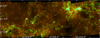 |
Fig. 1 Imageof SPIRE 250 μm emission showing an example of extracted sources around ℓ = 236° and b = − 1°. The image spans ~7° in longitude and ~3° in latitude. Overplotted are the sources identified by SExtractor (green ellipses). |
Astrometric data and integrated flux as determined by SExtractor for the extracted clumps for the first 20 clumps from a total of 23 817 sources.
Overview of the six dominating bright and complex regions and the number of sources taken into account in the present paper.
2.2 Observations
Carbon monoxide (CO) is the second most abundant molecule in the Milky Way after H2. It is widely found in molecular clouds, and even more so in the denser parts constituting the dusty clumps we investigated as part of this work. Observing the CO emission toward a dust clump allows us to obtain a velocity for a given clump and from this infer a distance to the clump. We used the facility receiver APEX-1 (SHeFI; Vassilev et al. 2008) at the Atacama Pathfinder Experiment 12 m submillimeter (submm) telescope (APEX; Güsten et al. 2006) to obtain line-of-sight velocities (vlsr) of the selected sources. Two wide-band fast Fourier transform spectrometers (FFTS; Klein et al. 2012) make up the back-ends, each consisting of 32,768 spectral channels covering an instantaneous bandwidth of 2.5 GHz. We targeted the 12CO(2–1) transition at230.5 GHz, as line-of-sight confusion is not as much an issue for the outer Galaxy than for the inner Galaxy, and the higher column densities allow for detection of sources at greater distances with similar integration times when compared to the rarer and less bright 13 CO(2–1) and C18 O(2–1) transitions. With this setup, we were able to observe the targeted transition at a velocity resolution of ~ 0.1 km s−1.
The observations toward 830 sources were conducted between July 2013 and December 2016 as a bad weather backup project at APEX with precipitable water vapour (PWV) up to 6 mm. To reach an rms < 0.1 K per channel, each source was observed in position switching mode for 3–6 min, depending on PWV, elevation, and line strength. The off-positions were selected as relative offsets with a separation of 1° roughly perpendicular to the Galactic plane. The pointed 12CO(2–1) observationswere obtained with an average PWV of 2.7 mm, resulting in an average rms of 0.05 K at a smoothed channel resolution of 1 km s−1. Sample spectra are shown in Fig. 4. In total, we found 37 spectra without any emission, leaving 759 (~91%) spectra for further analysis. A summary of all observational parameters is given in Table 3. To obtain CO(2–1) velocity information for each clump, we applied the methods described in the following section.
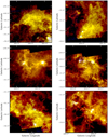 |
Fig. 2 Red-green-blue (RGB) images of the six brightest regions in the survey area. These have been excluded from the automated source selection to avoid biasing the survey toward these regions. Red: SPIRE 500 μm; Green: SPIRE 250 μm; Blue: PACS70 μm. |
2.3 Datareduction procedures
The obtained spectra were reduced using the Continuum and Line Analysis Single-dish Software (CLASS1). To obtain the velocity components from the observed spectra, we first combined all scans for a single observed position into a single spectrum. This was successively smoothed to a velocity resolution of 1 km s−1, and a linear baseline was subtracted. The spectra were then subjected to a Python code, where they were limited to the velocity range of −20 km s−1 < vlsr < 150 km s−1, in order to limit the spectra to velocity range expected for the outer Galaxy. Coherent groups of emission and absorption likely associated with a single cloud were determined by defining a window where all emission is above the 3σ noise level. These emission groups were then fit iteratively, starting with the brightest group. First the spectrum is de-spiked, after which point the number of peaks in a group is determined, Gaussian profiles are fit to the peaks, and the resulting fit is subtracted from the original spectrum. The procedure is then repeated until no residual emission above 3σ is found and all groups are fit. In order to avoid adding too many emission components that are close to each other and are likely associated with the same cloud, we only considered peaks separated by at least twice the width of the fit Gaussian as major emission components. The same process was repeated for negative emission features, allowing us to identify observations with a contaminated off-position.
In Fig. 4, we show example spectra of velocity measurements obtained toward sources located in the outer Galaxy. In the upper-left panel, a single emission component along the line of sight can be fit with a single Gaussian profile. This allows the velocity to be immediately assigned to the dust clump without further analysis. The situation becomes more difficult when a cloud is either composed of multiple components or there are multiple clouds located along the line of sight (Fig. 4, upper-right panel). Furthermore, as CO is the second most abundant molecule in the Milky Way, the reference position used when taking the spectrum might be contaminated, resulting in negative features in the spectrum (Fig. 4, lower-left panel). Contaminated spectra pose the problem that the emission might be at a similar velocity as the negative feature, thus rendering the velocities less reliable. In extreme cases, all three of these effects are present in a single spectrum (Fig. 4, lower-right panel).
Although these effects complicate the analysis, in most cases a velocity can still be assigned to the corresponding clump. Assuming that the emission as seen in the continuum maps is associated mainly with the brightest emission found in CO, only the CO emission with the highest integrated intensity is taken into account. If this CO cloud has an integrated intensity at least twice as high as the rest of the CO emission, we assume that the dust emission is associated with it. In case a negative feature is located close to it (d v < 1 km s−1), the uncertainty of the velocity measurement is increased by the width of the negative feature from the off-position, considering the velocity measurement is still usable but with a higher uncertainty.
With the line-of-sight velocity of a clump, we can determine its distance from the rotation curve of the Galaxy. As there is only one rotation direction in the southern outer Galaxy, namely from higher to lower longitudes, no distance ambiguity exists (in contrast to the inner Galaxy where this poses a problem), allowing for a direct conversion from the observed line-of-sight velocities to heliocentric distance.
We were able to fit spectra for 759 (91 %) of the 830 observed lines of sight, identifying a total of 982 clouds consisting of 1102 velocity components from the CO(2–1) emission above the 5σ level. From here on, we refer to a single fit Gaussian as a velocity component, and to any coherent group of emission as a cloud, as weassume that these groups of emission are physically connected with similar velocities but distinct components.
We found the source-off reference positions, selected as a relative offset from the target position of one degree, to be contaminated for 331 sources of the sample (39.9%), as shown for two lines of sight in the lower panels of Fig. 4. As the uncertainty in distances determined from the vlsr are mostly dominated by the uncertainty in the rotation curve used for the calculation rather than from the velocity, we assume that an uncertainty in vlsr of a few km s−1 (due to contamination in the source-off position) does not pose a serious problem. In fact, we conclude that the CO emission at the source-off position can be used to increase the number of positions for velocity measurements toward the outer Galaxy, but care has to be taken on their usage as discussed in the following paragraph.
Therefore, we also analyzed the emission at the off-positions when a source shows contamination. To do so, we simply invert the baseline corrected spectra and apply the same procedure as for the emission of uncontaminated sources, yielding velocity components for the off-position. We want to stress that these additional CO(2–1) clouds do not necessarily coincide with the peak of any dust clump or cloud, but as these components are clearly above the background noise level, they improve our view on the large-scale structures in the outer Galaxy. In contrast, for the spectral energy distribution (SED) analysis of the dust clumps in Sect. 3.1, we only take into account off-source positions that are matched with a SExtractor source position within one beam size (i.e., 30′′), yielding an additional 40 sources for which we can derive physical properties. If an absorption feature was found within 10 km s−1 of an emission peak, the uncertainties for all derived properties were increased by a factor of two (i.e., velocity, peak temperature, and line width). We choose a rather large range of 10 km s−1 in order to make sure that we also cover cases with broad emission complexes, where the emission between two peaks means they cancel each other out.
Analyzing the emission at the off-positions for the 331 contaminated spectra, we were able to add another 295 clouds above the 5σ noise level from 242 lines of sight to our analysis. This increases the total number of clouds by 23.1 % from 982 to 1277 consisting of a total of 1415 components and covering a total of 1090 lines of sight (targeted + reference). We present the results for each position in Table 4.
As observations were often conducted in poor weather conditions with high and fast varying PWV sometimes in excess of 5 mm, we only calculated the main-beam brightness temperature for sources that have a calibration within a certain time frame according to the weather conditions2, resulting in the removal of 23 lines of sight (29 clouds). For the remaining sources, the main beam temperature Tmb was then calculated from the antenna temperature  , multiplying with a forward efficiency of ηf = 95% and dividing by a beam efficiency of ηmb = 75%. In cases where no calibration was found within the given time frame, we do not give a main beam temperature or intensity.
For 966 (88.6%) lines of sight, only a single cloud is found, whereas multiple clouds are identified for 87 (11.4%) lines of sight. For 37 lines of sight, no emission was found. In summary, we identified a total of 1248 clouds for all 1090 lines of sight, yielding an average of 1.2 clouds each.
We give all clouds (i.e., groups of emission) in Table 5, which we define as continuous emission features above 3σ rms, consisting of one or more fit Gaussians. An example of two components (possibly arising from self absorption) making up one cloud can be seen in Fig. 4 (lower right) at ~80 km s−1 indicated by the solid black bar in the lower part of the figure. The velocity found for the brightest velocity complex along a given line of sight is laterused to assign a distance to the clump as seen in continuum emission, from which the physical parameters are derived.
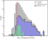 |
Fig. 3 Histogram showing integrated flux for the sources identified by SExtractor (gray) in comparison with those selected for our observations (blue) and those recovered from contaminated off-source positions (green; see Sect. 2.3). The red vertical dashed line indicates the limit of ~2.5 Jy that was imposed as a selection threshold (see text for details). |
Summary of the APEX observational parameters.
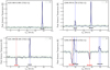 |
Fig. 4 12CO(2–1) spectra (black line) showing different typical profiles: single component (upper left), multiple components (upper right), simple contamination in the off-position (lower left), and a complex spectrum with all features (lower right). The total fit spectrum is overplotted in blue. Coherent velocity complexes are either marked as black (source position) or red (off position; negative features) horizontal bars below the spectrum. The vertical dashed blue lines indicate the peak positions of the fit Gaussian profiles, whereas the vertical red dashed lines indicate the peak position of the emission found in theoff-position. |
2.4 Source velocities
In Fig. 5, we present the longitude-velocity (ℓ-v) plot covering the observed field. The velocity components above the 5σ rms noise level for all positions are overlaid on the 12CO(1–0) emission data cube from Dame et al. (2001), integrated for − 3 deg ≤ b ≤ 0.5deg as approximately covered by our sample, that is, following the Galactic warp. The loci of the spiral arms as well as the local emission are indicated by the solid line (see Sect. 5.1 for details).
As can be seen, although we randomly sampled, components obtained for the CO(2–1) line trace all the major structures found in the CO(1–0) emission map very well. In addition, due to the 15-times-higher resolution of our pointed observations when compared to the data from Dame et al. (2001, i.e., 7.5′ versus 30′′), we are able to trace small structures that were previously missed, as these would fall below the detection limit due to beam dilution or blending with other clumps within the beam. For example, the structures with the highest velocity components at any given longitude would trace the most distant arm. The structure traced by our pointed observations from ℓ ≈ 242°, vlsr ≈ 60 km s−1 to ℓ ≈ 252°, vlsr ≈ 40 km s−1 is completely missed by the lower sensitivity CO(1–0) map. Additional features can be identified, indicating the structure between the spiral arms toward this region of the outer Galaxy to be more complex than indicated by the data from Dame et al. (2001). We discuss this in more detail in Sect. 5.
2.5 Kinematic distances and Galactic distribution
We determined distances for all velocity components by applying the Brand & Blitz (1993) rotation curve, assuming a distance to the Galactic center of R0 = 8.34 kpc and an orbital velocity of θ0 = 240 km s−1, as derived by Reid et al. (2014) and used by Urquhart et al. (2018). We prefer the rotation curve from Brand & Blitz (1993) over the more recent one from Reid et al. (2014), as the latter is derived from parallactic distances to objects visible from the northern hemisphere and does not include measurements for the southern outer Galaxy.
In Fig. 6, we show the distribution of our sources in the third Galactic quadrant as viewed fromthe Galactic north pole. We find the closest source to be located at a heliocentric distance of Rhel = 0.40 kpc, and the most distant sources at Rhel ~ 12 kpc. This resultsin the sources spanning a range of galactocentric distances between Rgal = 8.50 kpc and Rgal ~ 16.5 kpc. We note that the distances are not only affected by the uncertainty of the velocity measurement, but also by the spread due to streaming motions (≲10 km s−1; Reid et al. 2014), the expanding supershell (~7 km s−1; McClure-Griffiths et al. 2006), and the accuracy of the rotation curve, which can change the distance of any given source as determined from the rotation curve significantly (approximately ±1 kpc) and effectively dominating the uncertainty of the distance estimates.
In Fig. 7, we show the histogram of galactocentric (upper panel) and heliocentric (lower panel) distances for all velocity components above the 5σ rms noise level. The peaks are not only tracing the spiral arms, but also result from complexes lying at similar galactocentric distances. This can also be seen in Fig. 5, where the four peaks are marked by the colored dashed lines in the same way as in Fig. 7. We find that the peak located at rgal ~ 9 kpc traces local gas including emission from the Vela molecular ridge. The peak at ~11 kpc would trace the Perseus arm, if it were present in the area (see discussion in Sect. 5). The peaks around rgal ~ 12.5 kpc (cyan dashed line) trace emission not associated with a spiral arm, which is dominated by the huge complex at ℓ ~ 242° at vlsr ~ 70 km s−1 (i.e., behind the supershell; see Sect. 5.2). The peak found at rgal ~ 14 kpc partially arises from emission from the Outer arm as well as from structures between the Perseus and the Outer arm located at ℓ ~ 255°. Similarly, we see a number of peaks in the heliocentric distance histogram, but due to the projection these cannot be assigned to the arms, as the arms are spread out over a larger heliocentric distance range between 225° ≤ ℓ ≤ 260° than with regard to galactocentric distance.
Velocity components identified from the CO(2–1) observations along ten lines of sight.
Clouds (i.e., coherent groups of velocity components) identified from the CO(2–1) observations along a given line of sight for 15 complexes.
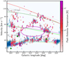 |
Fig. 5 Galactic longitude versus radial velocity. The dots mark all clouds found above 5σ rms between 260° ≤ ℓ ≤ 225°, with the peak antenna temperature color-coded. Background image: CO(1–0) emission from Dame et al. (2001). Dashed yellow, magenta, and green lines: peaks at 9, 11, and 14.0 kpc, respectively, as found in Fig. 7. The spiral arms and the position of the local emission as determined from H I emission are marked by the colored solid lines. Cyan: local emission; green: Perseus arm; red: outer arm. The solid magenta ellipse marks the rim of the Galactic supershell GSH 242-3+77. Gray dashed lines: galactocentric radii at 10 and 15 kpc. The green stars mark the positions of the three sources from the Methanol Multibeam (MMB; Green et al. 2012) survey found in the region. |
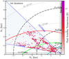 |
Fig. 6 Third quadrant of the Milky Way. The dots mark all clouds above 5σ rms, using the same color-coding as Fig. 5. The observed region (225° < ℓ < 260°) is highlighted in light blue. Heliocentric distances d and galactocentric radii R are indicated as dash-dotted black and dotted gray circles, respectively. Positions of arms and local emission are indicated by solid lines in the same colors as in Fig. 5. The position of the Galactic supershell GSH 242-3+37 is indicated by the magenta ellipse. From the observed vlsr we calculated the heliocentric distances for each cloud using the Brand & Blitz (1993) rotation curve to obtain Galactic positions. |
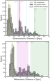 |
Fig. 7 Histograms showing CO velocity components above 5σ (light gray), CO emission groups/clouds (dark gray) and matched dust clumps (black outline) by galactocentric (upper) and heliocentric (lower) distance. The vertical dashed yellow line indicates the peak associated with local emission. The magenta and green shaded areas mark the distance range between 225° ≤ ℓ≤ 260° of theloci of the Perseus and Outer arms, respectively. The two peaks between rgal ~ 12 and ~ 13 kpc correspond to complexes between the Perseus and Outer arm. |
3 Physical properties
We now investigate the physical properties that can be derived from archival mid-infrared to submm continuum emission data in combination with the distances obtained from our pointed CO observations (Sect. 2.5). First, we discuss how we obtained the dust spectral energy distributions for the outer Galaxy. We then present the derived physical properties and investigate how consistent they are, followed by a detailed look at the results. Here, we mainly investigate the star formation relations, as well as the influence of the main structures present in the outer Galaxy on the physical properties of the observed clumps.
Source parameters obtained from the SEDs for the first 15 sources.
3.1 Dust spectral energy distributions
To obtain and fit the dust spectral energy distributions (SEDs), we followed the procedures we described in detail in König et al. (2017) and Urquhart et al. (2018), hence we only give a brief overview here.
We usedarchival mid-infrared to submm continuum maps to obtain the SEDs in nine different bands at 8, 12, 14, 21/22, 70, 160, 250, 350, and 500μm. In contrast to our previous work, there is no ATLASGAL data available at 870 μm for the outer Galaxy, so we used the 250 μm positions and source sizes obtained from the source extraction process described in Sect. 2 for the photometry. In the far-infrared to submm regime, we used Herschel/Hi-GAL (Molinari et al. 2010), PACS (Poglitsch et al. 2010), and SPIRE (Griffin et al. 2010) emission maps, covering the cold dust emission from 70 μm to 500 μm. This data is complemented by mid-infrared maps from WISE (Wright et al. 2010) and MSX (Price et al. 2001) covering the wavelength regime between 8 μm and 22 μm, which is mostly dominated by the emission of a hot embedded component of (proto-)stars. The fluxes for each band are obtained through aperture photometry as described in detail in our previous work (Urquhart et al. 2018), reconstructing the SED of each source. Whenever a flux was measured in the WISE emission maps at the 12 or 22 μm bands, it was preferred over the corresponding fluxes at 12 or 21 μm determined for the MSX bands due to the lower noise level and moderately better resolution of the WISE images. In this way, we obtainedSEDs for all observed positions as well as for off-positions that were matched with the extracted sources.
We fit the SEDs using a single-component gray-body or two-component model, depending on the emission in the mid-infrared bands. A sample two-component SED is shown in Fig. 8. In contrast to our previous work, we used the emission found in the 350 μm SPIRE band as the reference wavelength due to the absence of a flux measurement at 870 μm. In total, we were able to fit 611 SEDs (~77%) of the 791 sources. The SEDs for 180 sources were not recovered completely due to either sensitivity, the source being located in a crowded region, the SED being irregular, or the source being too close to the edge of the Hi-GAL area (or a combination of those). We summarize the parameters used to obtain the SEDs and the fit parameters (dust temperature and opacity) in Table 6 alongside the evolutionary classes as determined from the SEDs (see Sect. 4.1).
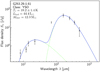 |
Fig. 8 Sample SED (G253.29-1.61) with hot and cold components, classifying this source as a young stellar object (YSO). |
3.2 Deriving physical properties
Using the dust temperatures from the fit SEDs and assigning distances as determined in Sect. 2.5, we calculated the physical properties from the SEDs as described in König et al. (2017). However, as the reference wavelength has changed to the S350 SPIRE band, slight changes were made to how we calculated the clump mass and H2 column density. We obtained theclump mass Mclump from the integrated 350 μm flux density S350 as
Physical parameters derived from the dust SEDs for the first 15 sources.
 (1)
(1)
where d is the distance to the source, B350(Td) the intensity of a blackbody at 350 μm at the cold dust envelope temperature Tc. The dust opacity κ350 = 1.1 cm2g−1 at 350 μm is calculated as the mean of all dust models from Ossenkopf & Henning (1994), using the dust emissivity index of β = 1.75 used for fitting all SEDs.
As the gas-to-dust ratio γ increases with galactocentric distance, due to the decreasing metallicity in the outer Galaxy we apply a correction factor according to the recently determined trend by Giannetti et al. (2017a, Eq. (2)):
![Mathematical equation: \begin{eqnarray*} \log \gamma\,{=}\,0.087 \cdot \frac{R_{\mathrm{gal}}}{\mathrm{[kpc]}} + 1.44 .\end{eqnarray*}](/articles/aa/full_html/2021/01/aa39523-20/aa39523-20-eq3.png) (2)
(2)
Here, alinear slope is applied to the logarithm of the gas-to-dust ratio γ, increasing the factor from γ ~ 150 near the solar circle to γ ~ 550 at 15 kpc galactocentric radius. We point out that without this correction the clump masses in the outer Galaxy would be underestimated by up to a factor of five compared to masses calculated using the widely adopted value of 100 for the gas-to-dust ratio for the inner Galaxy. Similarly, we adopt the calculation of the column density  to the reference wavelength of 350 μm:
 (3)
(3)
were F350 is the peak flux density, Ωapp the beam solid angle, and  the mean molecular weight of the interstellar medium with respect to a hydrogen molecule (Kauffmann et al. 2008) and mH the mass of a hydrogen atom.
We summarize the physical properties derived from the dust emission for each source in Table 7. A summary of the dust properties, also taking into account their evolutionary stage (Sect. 4.1), can be found in Table 8. We discuss the physical properties in detail and put them into context of their Galactic environment in the following sections.
3.3 Consistency checks
To check the consistency of our method, we compared the  column densities derived from the SEDs with column densities derived from the 12CO(2–1) emission. To obtain the column densities from 12CO(2–1), we calculatethem as
 (4)
(4)
where we used the H2-to-CO conversion factor of  cm−2 (km s−1)−1 obtained by Brand & Wouterloot (1995) for the outer Galaxy, and the integrated line intensity I(12CO(2-1)) as measured from the observed spectra with a line ratio of 12CO(2–1)/12CO(1–0) = 0.7 (Sandstrom et al. 2013). In the upper panel of Fig. 9, we show the comparison of the column densities derived from dust and CO. As the CO(2–1) column density is derived from emission measured within a beam of 30′′, it traces the denser regions of the more extended clumps with an average angular source size of 62′′, resulting in slightly higher column densities when compared to those derived from the dust emission. Nevertheless, we find both quantities to be in good agreement (p-value of 0.0155) although a large scatter is observed.
We also compare our results to a similar sample of southern outer Galaxy sources from Elia et al. (2013) obtained for an adjacent area of the southern sky (216.5° < ℓ < 225.5°). In the lower panel of Fig. 9, we compare the clump masses as derived from the Herschel dust continuum emission of both samples. Similarly to the masses calculated for our sample, we applied a correction factor for the varying gas-to-dust ratio found by Giannetti et al. (2017a) to the masses calculated by Elia et al. (2013). We find the distribution to be statistically different (p-value of 5.3 × 10⁻⁴), with the sample of the present work picking up significantly more lower mass sources. This is reflected by the mean values to be almost identical with values of 58.2 ± 6.0 and 56.8 ± 5.4M⊙ for our sample and the Elia et al. (2013) sample, respectively, but the median values to differ by a factor of 1.6 (10.1 and 16.2 M⊙, respectively). The difference for these two samples is likely caused by a combination of two effects. First, the areas are non-overlapping, so the differences might reflect intrinsic differences of the two areas covered in the outer Galaxy, especially when taking into account the Galactic supershell GSH242-03+37 covered in the present work (see Sect. 5.2). Furthermore, the distances for the sample by Elia et al. (2013) were obtained with the NANTEN 4 m telescope with a beam size of 2.6′ (Kim et al. 2004), only allowing us to assign distances to the brighter sources within the beam.
From the comparison with the column densities derived from 12CO as well as with the clump masses from Elia et al. (2013), we conclude that our methods can be considered reliable, as either the distributions are similar, as shown by an Anderson-Darling test, or they agree on average within the margin of error.
Summary of physical properties of the whole population of clumps and the three evolutionary subsamples identified.
3.4 Distance biases
Some physical properties suffer from observational distance biases, such as the bolometric luminosity, clump mass, and linear source size. These biases are caused by the fixed sensitivity and resolution of the telescope/instrument used. Due to the limited sensitivity, only the brightest and most massive sources can be observed at the farthest distances. Similarly, the limited angular resolution only allows us to observe sources down to this apparent size, which at farther distances translates to larger linear source sizes. To avoid misleading trends that are introduced by these sensitivity and resolution-based selection biases, we determined a completeness limit, above which the survey does not suffer from these selection effects out to the given distance.
First, we need to distinguish between distance-independent parameters and distance-dependent parameters. The dust temperature, peak column density, and L∕M are distance independent, as they are either intrinsic to the sources or cancel out the distance dependence. As mentioned in the last paragraph, the bolometric luminosity and clump mass are directly scaled by the distance squared, and hence are highly dependent on correct distances and are prone to distance-dependent observational biases. The same is true for the linear source size, which is linearly dependent on the distance.
To determine in which mass and luminosity range our survey does not suffer from distance biases, we show the distribution of luminosities, masses, and linear source sizes with respect to heliocentric distance in Fig. 10. We calculated the theoretical sensitivity according to Eqs. (1) and (2) in König et al. (2017) for the bolometric luminosity and clump mass from the minimum values as input parameters, varying the distance. Similarly, we calculated the resolution limit from Eq. (3) in König et al. (2017) but used the beam size for SPIRE 250 (18.2′′) as input parameter. The theoretical sensitivity and resolution limits are plotted as green solid lines in Fig. 10.
As the source count of our sample drops significantly beyond 9 kpc heliocentric distance, we estimate the completeness limit up to this distance as the value of the theoretical sensitivity or resolution limit at 9 kpc. For the bolometric luminosity, we find that sources out to ~9 kpc distance arestrongly affected by the sensitivity of this survey for luminosities below 6.5 L⊙. Masses of 9 M⊙ are found to be the completeness limit for clump mass, whereas for the linear source size, sources smaller than 0.23 pc suffer from the distance bias. We filter our samples according to these completeness limits when analysing the distance dependent physical properties.
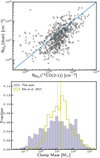 |
Fig. 9 Consistency checks. Top: comparing peak N |

4 Discussion
In this section, we discuss the physical properties derived in the previous section. We put a focus on the analysis of the properties found in theouter Galaxy with respect to the structures found here.
4.1 Evolutionary sequence
Based on the flux densities obtained for the SEDs, we determine the evolutionary state of the sources, following the classification scheme introduced in König et al. (2017), which was also used by Urquhart et al. (2018) for the entire ATLASGAL sample.
We follow here the naming scheme of our latest paper and refer to mid-infrared bright sources as young stellar objects (YSOs). We note, however, that these might also include some compact H II regions, which we did not identify individually. We therefore refer to the following three classes:
- (i)
Quiescent sources, which are dark at 70 μm (no compact emission at 70 μm) and represent the earliest phase of star-formation in our sample. These sources might or might not be collapsing.
- (ii)
Protostellar sources, which are bright at far-infrared and submm wavelengths but are not sufficiently evolved to produce significant emission at mid-infrared wavelengths (F20 ≤ 0.1 Jy)3. These sources are in the process of collapse and are internally heated.
- (iii)
Young stellar objects, which are bright at mid-infrared wavelengths (F20 > 0.1 Jy). This group of sources is significantly evolved to produce strong emission at mid-infrared wavelengths by an internal heating source.
This classification scheme has been proven to be reliable as shown by Giannetti et al. (2017b) using molecular line data. It was further bolstered by our recent work on the ATLASGAL sample (Urquhart et al. 2018), showing clear trends of increasing dust temperature, and of the bolometric luminosity clumping mass ratio, proving this evolutionary sequence. Cumulative histograms for the dust properties and the three evolutionary phases of all sources are shown in Fig. 11. Again, we find the evolutionary stages to be well separated from each other for the dust temperature, the bolometric luminosity, and the luminosity-to-mass ratio, as found in König et al. (2017) for the Top100 sample4.
This reflects the increase in luminosity due to the accretion of material onto the protocluster and the heating of the local environmentas the protostars evolve (compare Sect. 4.3 and Molinari et al. 2008). The similarity between the three evolutionary classes was determined by Anderson-Darling tests, indicating the distributions to be significantly different for each of the aforementioned physical properties, as their pairwise p-values are all well below the threshold of p < 0.0013, corresponding to a 3σ confidence. These three properties (dust temperature, bolometric luminosity, and luminosity-to-mass ratio) are therefore excellent indicators of the evolutionary phase of a clump. Care has to be taken though, as there is a large overlap between the different phases, and therefore we can not simply read the evolutionary phase of a single clump by only taking into account these numbers. However, they can be used to determine statistical properties and identify significant trends in the data.
For theremaining three physical properties (clump mass, linear source size, and H2 column density), the quiescent and protostellar evolutionary stages are indistinguishable with a p-value of 0.1. Only the clumps in the YSO phase show, on average, slightly higher values of these properties than the two earlier phases with p-values below 1.8 × 10⁻⁴. This indicates that the classification scheme tends to identify the larger, more massive clumps as being more evolved, indicating that the more massive clumps evolve significantly faster than their low-mass counterparts.
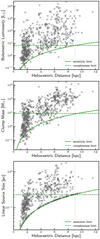 |
Fig. 10 Observational distance biases. Bolometric luminosity (top), clump mass (middle), and linear source size (bottom) versus heliocentric distance. The solid lines mark the distance-dependent sensitivity/resolution limit. The horizontally dashed green lines mark the limit above which our survey does not suffer from a distance bias up to 9 kpc (vertical dotted line). |
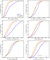 |
Fig. 11 Cumulative distributions for derived parameters of this survey. Colored lines indicate the distribution for the different evolutionary phases, whereas the dark gray line represents the full sample. |
4.2 Physical properties
Temperatures and optical depth
Temperature and optical depth are determined as fit parameters from the SEDs and are distance independent. We find that the dust temperatures range from 9.65 to 41.31 K with a mean value of 17.29 K. We point out that our sample has, on average, a 2 K lower mean temperature when compared to Urquhart et al. (2018), probably arising from the difference in sensitivity of the two surveys. We therefore leave a detailed comparison for Paper II. For the optical depth, we find that all of our sources are optically thin (τ ≪ 1) at 350 μm, as the optical depths range from 1.9 × 10⁻⁶ up to a maximum of 2.9 × 10⁻³.
Source sizes
In the lower-left panel of Fig. 11, we show the distribution of linear source sizes for our sample. Linear source sizes derived from the apparent full width at half maximum source size vary between 0.03 and 1.78 pc, yielding a mean source size of 0.25 pc. This is almost identical to the value of 3.2 × 10⁻¹ pc for the ATLASGAL sample in the first and fourth Galactic quadrants (Urquhart et al. 2018), showing that both samples trace structures of similar scales, allowing for a detailed comparison of the different samples.
H2 column density
The peak H2 column density is found to range between 6.3 × 1019 cm−2 and 4.1 × 1022 cm−2 with a mean value of 3.8 × 1021 cm−2 in the outer Galaxy. As this is below the 1023 cm−2 found by Urquhart et al. (2018) above which almost all clumps are associated with high-mass star formation, we expect to find significantly less massive clumps in the outer Galaxy.
Bolometric luminosity and clump mass
The bolometric luminosities for the outer Galaxy sample range between 8.0 × 10⁻² L⊙ and 2.4 × 10⁴ L⊙, with a mean value of 3.6 × 10² L⊙. Clump masses range from 2.3 × 10⁻² M⊙ to 1.7 × 10³ M⊙, with a meanvalue of 58 M⊙. As with the H2 column density, we expect from these maximum values only a small number of sources to be able to form high-mass stars, which we investigate in the following sections.
4.3 Star formation relations
In Fig. 12, we show the bolometric luminosity plotted versus the clump mass. For a given clump, one expects the luminosity to increase during the accretion phase, hence moving upward in the figure until stars reach the zero-age main sequence (diagonal solid line). As soon as stars are formed, their feedback disrupts a given clump. As a consequence, the clump is dispersed, decreasing its mass, and hence moving left in the diagram. These evolutionary paths through the diagram are indicated by the gray tracks, as calculated by Molinari et al. (2008). In order to visualize the differences between the evolutionary phases as described in Sect. 4.1, we show the linear fits to the evolutionary classes as dash-dotted lines. As can be seen, the sources of the different classes move up in the plot as expected from the evolutionary scheme described in Sect. 4.1. This trend is consistent with the cumulative distribution of the bolometric luminosity-to-clump mass ratio L⊙ /M⊙ shown in the lower-right panel of Fig. 11. There we find the three classes to be well separated, with all p-values well below 0.0013, following the expected evolutionary trend. Furthermore, we indicate the expected luminosity for a B2 star (~ 8M⊙) as calculated by Mottram et al. (2011) as a dashed horizontal line. Above this threshold, we assume that at least one massive star has formed in the clump that is responsible for most of its luminosity, but we point out that this threshold only sets an upper limit for the number of high-mass stars according to our criterion. The vertical dashed line marks the clump mass threshold above which it is likely that the clumps host massive dense cores or a high-mass protostar (Csengeri et al. 2014). From these thresholds, we see that only the minority of the sources in the outer Galaxy are able to form a high-mass star (32 sources), and the majority of these have already done so (24 sources at most).
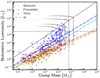 |
Fig. 12 Bolometric luminosity versus clump mass. The gray tracks indicate the evolutionary path through the diagram for the given initial masses as calculated by Molinari et al. (2008). The diagonal solid line marks the expected luminosity for a given mass for a zero-age main-sequence (ZAMS) star. The horizontal dashed line indicates the expected luminosity for a B2 star (~ 8M⊙) as calculated by Mottram et al. (2011). The vertical dashed line marks the threshold calculated by Csengeri et al. (2014) above whichthe clumps are likely to host massive dense cores or a high-mass protostar. The dash-dotted lines are linear fits to the three evolutionary classes. |
4.4 Mass-size relation
In Fig. 13, we show the clump mass plotted versus the source radius. The gray dotted line marks the mass limit for high-mass stars at 8 M⊙. The gray shaded area marks the regime where supposedly only low-mass stars form, as determined by Kauffmann et al. (2010), with only 40 sources (7%) of the outer Galaxy sample above the threshold and the mass limit. The black dashed line marks the lower limit for effective high-mass star formation as determined by Urquhart et al. (2014c), indicating a surface density threshold of 0.05 g cm−2 found for the inner Galaxy using the ATLASGAL survey. One hundred and forty of our sources (i.e., 23%) are found above this threshold and the mass limit for high-mass stars. Although we find the majority of the clumps to be able to form only low-mass stars, as we did in the last section, we find a significantly higher fraction potentially form high-mass stars according to the latter threshold used here. As a consequence, we speculate that the threshold for high-mass star formation based on mass surface density is likely to be different in the inner and outer Galaxy, as the radial mass surface density profile of the Galaxy drops significantly according to the review by Heyer & Dame (2015, Fig. 7).
Finally, we compare the evolutionary phases (color-coded), but no trend with regard to the evolutionary state of the clumps is found, as can be seen from the linear fits to the individual classes (colored dash-dotted lines). This is in agreement with our findings in Sect. 4.1.
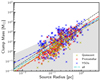 |
Fig. 13 Clump mass versus source radius. The shaded area marks the regime where only low-mass stars form, as determined by Kauffmann et al. (2010). The black dashed line marks the lower limit for effective high-mass star formation as determined by Urquhart et al. (2014c), indicating a surface density threshold of 0.05 g cm−2. The horizontal gray dotted line marks the threshold of 8 M⊙, above whicha clump is considered massive. The colored dash-dotted lines are linear fits to the corresponding subsamples, and the cyan dash-dotted line is a fit to the full sample. |
4.5 Independent high-mass star formation tracers
To further identify high-mass star forming clumps, we also investigated the presence of methanol Class II masers as identified by the Methanol MultiBeam survey (MMB; Green et al. 2012), which are thought to be exclusively associated with objects in the early phasesof high-mass star formation (Urquhart et al. 2015). In the whole area of our survey, only two methanol Class II masers are found (G254.880+0.451 and G259.939-0.041), indicating either a lower rate of high-mass star formation, or that they result from the lower metallicity toward the outer Galaxy (Lemasle et al. 2018), thus reducing the available amount of methanol CH3OH, which contains two metal atoms.
Therefore, we also investigated the number of H II regions in the survey area as identified by the Red MSX Survey (RMS; Lumsden et al. 2013) and the WISE catalog of Galactic H II regions (Anderson et al. 2014), as the formation of H II regions is independent of the metallicity. Merging both catalogs, we find ten known H II regions in our survey area (three from the RMS survey, eight from the WISE catalog, with one source in both), as well as another 24 candidate H II regions from the WISE catalog. These are about a factor of 20–30 fewer sources per unit area as compared to the inner Milky Way for the aforementioned surveys.
As these numbers are in the same order as the results from our dust continuum emission in the previous paragraphs, we conclude that there is only very limited high-mass star formation occurring in the outer Galaxy.
5 Structure of the outer Galaxy
In this section, we use the distance information as derived from the radial velocities to give an overview of the structure of the area investigated in this work. We briefly investigate the spiral structure as found toward the third Galactic quadrant and look into the influence of a Galactic supershell known to exist in the observed region.
5.1 Spiral arms and inter-arm regions
The nature of the structure of the Milky Way is still under debate (Dobbs & Baba 2014), and it is unclear weather it is a ‘flocculent’ or ‘grand-design’ spiral galaxy. The existence of four spiral arms would denominate it as a flocculent galaxy, whereas a grand design interpretation would leave the Galaxy with two density wave arms (Perseus and Scutum-Centaurus) and the others as transient features. For this reason, the location and visibility of the spiral arms toward the observed Galactic quadrant is also still under debate with either a single arm or two arms visible (compare e.g., Reid et al. 2014, 2016; Koo et al. 2017). Here we focus on a model where both the Perseus arm and the Outer arm are found in the southern outer Galaxy, as the Outer arm is clearly present in the H I emission (compare Fig. 14). However, the location of the arms in the third Galactic quadrant is not well constrained, as their loci are extrapolated from the northern hemisphere, where the measurements of spiral arm positions are better constrained.
We show a larger region toward the outer Galaxy in Fig. 14, covering Galactic longitudes 215° < ℓ < 280° as mapped in H I by the Galactic All Sky HI Survey (GASS; McClure-Griffiths et al. 2009). To plot the loci of the spiral arms, we used the equation for a log-periodic spiral, as described in Reid et al. (2014):
 (5)
(5)
where Rgal is the galactocentric radius, Rref the galactocentric radius at the reference galactocentric azimuth βref (with βref = 0 toward the sun, increasing with Galactic longitude), and the pitch angle Ψ. In Fig. 14, we indicate the extrapolation of the spiral arms and Orion/Local spur as determined by Reid et al. (2014) and Reid et al. (2019) from trigonometric parallax measurements for the northern hemisphere as dashed lines. This includes (from low to high vlsr) the Orion/Local spur, the Perseus arm and the Outer arm. Furthermore, we plot the two arms visible in the third Galactic quadrant from the four-arm model as determined as the average in several publications by Vallée (2015) as dash-dotted lines. Although the extrapolations for the Perseus spiral arm are all still in good agreement, the extrapolations for the Outer arm deviate quite drastically from each other (esp. Reid et al. 2019) due to the high uncertainties involved, and fail to trace the highest column density H I emissions in the present region.
Therefore we also plot our own estimates as solid lines for the three main features (from low vlsr to high vlsr): local emission from the Vela molecular ridge (lower left) to the Orion/Local spur (lower right), the Perseus arm (middle) and the Outer arm (upper). As a detailed analysis of the position of the spiral arms is out of the scope of this work, we manually modified the spiral arm parameters so as to visually match the densest emission as seen in the H I integrated intensity map.
We note that the local emission (Vela molecular ridge and Orion/Local spur) is an inter-arm feature between the Sagitarius spiral arm located in the inner Galaxy at Rgal ~ 7 kpc and ℓ = 0° (not visible here) and the outer Galaxy. The position indicated here by the solid cyan line therefore does not represent an arm that is part of the spiral pattern, but just a fit to the local emission. In the case of the Vela molecular ridge, the emission distribution bends inward with increasing Galactic azimuth with a large negative pitch angle, in contrast with the spiral arms extending outward with increasing Galactic azimuth and a comparably smaller pitch angle. The parameters used for the spiral arms and the local emission are summarized in Table 9.
To give an overview and explore the three-dimensional structure of the observed region, we present longitude-velocity (ℓ −v) plots for different slices of Galactic latitude in Fig. 15 and latitude-velocity (b − v) plots for different slices of Galactic longitude in Figs. 16 and 17. We show the H I integrated intensity as a background image (McClure-Griffiths et al. 2009), the CO(1–0) emission from Dame et al. (2001) as black contours, and we mark the positions of our sources observed in CO(2–1) as small crosses with those associated with dust clumps as colored dots. We now discuss the different features present in the area.
We find that our sources as detected in 12CO(2–1) are mostly well correlated with the brightest features of the H I emission. They trace the local emission very well, but aside from the region of the brightest H I emission located at ℓ ~ 233°, they trace the Perseus arm poorly. We conclude that this is not a sensitivity issue, as plenty of sources between vlsr ~ 80-90 km s−1 are well detected in the ℓ ~ 258° region, and therefore we find no reason why such sources should not be detected in the Perseus arm between 225° < ℓ < 250°. Similarly, we find the CO(2–1) emission to be poorly correlated with the Perseus arm for some slices of longitude (ℓ ~ 254° and ℓ ~ 227°; Fig. 16, right panels). We conclude that the poor coherence of the observed source velocities with the locus of the Perseus arm in ℓ − v and b − v plots is a consequence of the presence of the expanding Galactic supershell G 242-03+37, which we investigate further in Sect. 5.2.
Several larger features can be identified spanning between the local emission and the suspected positions of the spiral arms (compare Fig. 15): in the region toward higher longitudes than the supershell (250° < ℓ < 260°), a web-like network of blobs, bridges, or spurs can be seen, with large clusters of clumps correlated with the brightest H I emission. At least four such complexes can be identified by eye from the ℓ − v maps (ℓ ~ 254°, vlsr ~ 38 km s−1; ℓ ~ 257.5°, vlsr ~ 50 km s−1; ℓ ~ 258°, vlsr ~ 80 km s−1; ℓ ~ 259°, vlsr ~ 60 km s−1), with more isolated clumps along the bridges. These bridges are also well visible in the b − v plot around ℓ ~ 285.5° (Fig. 16, upper-right panel). We note that these bridges might not be visible in CO(1–0), as the sensitivity is rather poor (rms noise up to 0.4 K).
Between225° < ℓ < 240° (i.e., lower longitudes than the supershell), we find at the lower latitudes (see right-hand column of Fig. 15) a feature in H I that is aligned perpendicular to the line of sight, indicating the continuation of the Perseus arm from the north. However, for higher latitudes (left-hand column of Fig. 15), this structure becomes more complex with a network of bridges spanning between the Orion/Local spur, and the Outer arm is more parallel to the line of sight (and perpendicular to the arms). This can also be seen in the b − v plot in Fig. 16 (lower-left panel), where the CO emission at b ~ 0° spans from vlsr ~ 20 km s−1 out to vlsr ~ 60 km s−1, whereas the local emission and the Perseus and Outer arms are more clearly separated at lower latitudes. This change in morphology and the orientation in dependence on the Galactic latitude could either be interpreted as the Perseus arm being disrupted or this structure not being a spiral arm at all. In contrast to the web of structures located toward higher longitudes than the supershell between 250° and 260°, we only find one larger star forming complex in this area (ℓ ~ 232°, vlsr ~ 50 km s−1), located at the rim of the supershell (Fig. 17).
In general, we find the three-dimensional structure of the Galactic disk toward the outer Galaxy in the third quadrant to be rather complex; not only with respect to longitude and velocity/distance, but also with respect to the vertical structure of the thin disk. The structures found in the observed region change rather dramatically with Galactic latitude, showing that the thin disk is more a complex three-dimensional web-like structure than a flat, pancake-like structure.
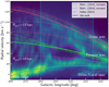 |
Fig. 14 HI emission from the Galactic All Sky HI Survey (GASS; McClure-Griffiths et al. 2009) for a larger region of the outer Galaxy covering 215° < ℓ < 280° indicating the integrated brightness temperature between − 5° < b < 1.5°. Overplottedare the positions of the spiral arms from Reid et al. (2014, 2019), and Vallée (2015) as dashed, dotted, and dash-dotted lines, respectively. The spiral arms and local emission as determined in the present work are marked by the solid lines. The dotted gray lines mark galactocentric radii at 10 and 15 kpc. the solid magenta ellipse marks the position of the Galactic supershell GSH 242-3+37. The light blue area framed by the blue dotted lines marks the area of the present work. |
Spiral arm parameters.
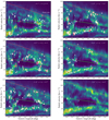 |
Fig. 15 Galactic longitude versus radial velocity integrated for slices of Galactic latitude. Latitude ranges from b = + 0.5° (top left panel) to b = −3.0° (lower right panel). Crosses mark the CO(2–1) velocity components along a line-of-sight, with colored dots indicating associated dust clumps. Sizes correspond to the integrated line intensity and the colors for the dust clumps to the 22 μm WISE emission being indicative of ongoing star formation. The background image shows the corresponding H I integrated intensity from the GASS survey (McClure-Griffiths et al. 2004). The contours mark the CO(1–0) emission from Dame et al. (2001) at levels of 3σ, 5σ, 7σ and the 10th, 30th, 50th and 70th percentile. The spiral arms as determined in the present work and the position of the local emission are marked by the colored solid lines. Cyan: local emission; green: Perseus arm; red: outer arm. The solid magenta ellipse marks the position of the Galactic supershell GSH 242-3+37. |
5.2 The Galactic supershell GSH 242–03+37
One of the most striking features toward the observed region is the void located at ℓ ~ 242° and vlsr ~ 40 km s−1. This structure is known to be the Galactic supershell GSH 242–03+37 and was first identified by Heiles (1979), and it was more recently investigated by McClure-Griffiths et al. (2006). It has a diameter of the order of a kiloparsec and an expansion velocity of ~7 km s−1. With the shell spanning about 15° in Galactic longitude, 25 km s−1 in velocity, andbeing centered − 1.6° below the Galacticplane, we find that our observed region spans roughly a band around the equator of that supershell.
As this structure has a profound impact on this region, we briefly discuss the possible origin of this supershell. McClure-Griffiths et al. (2006) calculated the energy needed to form such an expanding supershell to be of the order of 1053 ergs, which is about two orders of magnitude higher than the expected energy input from a single Type II supernova (Woltjer 1974). This would therefore require of the order of hundreds of Type II supernovae to drive this shell, which is rather unlikely, especially as there is no strong X-ray source at the center of the shell, which would be expected in the presence of hundreds of expected supernova remnants. A more suitable explanation might be the passage of a high velocity cloud (HVC) through the Galactic disk, like the one observed by Park et al. (2016) causing the Galactic shell GS040.2+00.6-70 in the northern hemisphere. Furthermore, HVCs are known to punch holes through galactic disks (e.g., Schulman 1996; Boomsma et al. 2008). Preliminary literature research further bolsters this hypothesis (compare e.g., Galyardt & Shelton 2016; McClure-Griffiths et al. 2006; Planck Collaboration Int. XIX 2015), but as an investigation of the origin of this shell is out of the scope of this work, we instead continue to discuss its impact on the region.
A consequence of the existence of this huge expanding supershell is a reduced reliability of kinematic distances for sources within its vicinity, as the expansion of the shell at a velocity of vexp ~ 7 km s−1 (McClure-Griffiths et al. 2006)distorts the Galactic rotation curve. For the distances to the shell’s center, this mostly affects the sources at the front and rear walls of the supershell, as the line-of-sight velocity vlsr is parallel to the expansion velocity vexp. However, the expansion velocity vexp has no effect on the sources on the northern or southern edges of the shell, as their position relative to the center of the shell is measured from the longitude and the line-of-sight velocity vlsr is not affected as it is perpendicular to the expansion velocity. The effect can be seen in Fig. 6 as the supposedly circular supershell is deformed into an ellipse along the line of sight. Accordingly, this needs to be taken into account when interpreting structures, and especially spiral arms in this region of the Milky Way. Furthermore, the supershell is coincident with the extrapolation of the Perseus arm, which might be the main reason why the Perseus arm cannot be traced clearly in this part of the outer Galaxy. If a large high-velocity cloud has hit the Perseus arm in the past, such an event might simply have lead to its local destruction, pushing the material of the arm away. Indeed, we see a ring of sources identified in CO emission around this supershell.
In Fig. 18, we present a histogram of the number of CO emission components, clouds, and associated dust clumps versus the center of the supershell normalized by the area. With the Galactic plane being coincident with the rim around the equator GSH 242–03+37, we find the central region (rGSH ≤ 0.4 kpc) void of any clumps. However, we find that the number density of sources is increased in the wall of this supershell between 0.6 kpc ≤ rGSH ≤ 1.2 kpc, which we estimate to be ~0.6 kpc wide. In fact, we find a sharp increase in number density of clumps from the inner void to the wall, which then gradually falls off again5. This is in agreement with McClure-Griffiths et al. (2006), who found a sharp increase in H I from the inner region to the wall of the shell, interpreting it as an indication of compression associated with a shock.
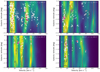 |
Fig. 16 Selected slices of Galactic latitude versus radial velocity integrated over 3° in Galactic longitude away from the Galactic supershell (top: higher longitudes than shell, bottom: lower longitudes of the shell). Crosses mark the CO(2–1) velocity components along a line of sight, with colored dots indicating associated dust clumps. Sizes correspond to the integrated line intensity and the colors reflect ongoing star formation as indicated by the 22 μm WISE emission. The background image shows the corresponding H I integrated intensity from the GASS survey (McClure-Griffiths et al. 2004). The contours mark the CO(1–0) emission from Dame et al. (2001) at levels of 5σ, 7σ, and the 10th, 30th, 50th and 70th percentiles. The spiral arms as determined in the present work and the position of the local emission are marked by the colored solid lines. Cyan: local emission; green: Perseus arm; red: outer arm. |
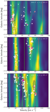 |
Fig. 17 Slices of Galactic latitude versus radial velocity integrated over 3° in Galactic longitude at the edges (top, bottom) and the center (middle) of the Galactic supershell. Colored dots mark the positions of the dust clumps, and white crosses mark the positions of clouds identified by the CO(2–1) pointed observations that are not associated with the dust clump. The background image shows the corresponding H I integrated intensity from the GASS survey (McClure-Griffiths et al. 2004). The contours mark the CO(1–0) emission from Dame et al. (2001) at levels of 5σ, 7σ, and the 10th, 30th, 50th and 70th percentiles. The spiral arms as determined in the present work and the position of the local emission are marked by the colored solid lines. Cyan: local emission; green: Perseus arm; red: outer arm. |
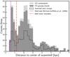 |
Fig. 18 Histogram for distance of all clouds identified in CO to the center of the supershell. The edge of the supershell is clearly distinguishable from the other sources, with the central parts at R < 0.4 kpc being void of any CO clouds. |
5.3 Physical properties with respect to the Galactic supershell
In the previous section, we examined the distribution of clumps around the supershell. In this section, we consider the impact of the supershell on its environment.
To avoid observational and selection biases, we limited our sample to only include sources that are symmetrically distributed around the shell with a maximum distance of 2.5 kpc to its center, reducing our sample size to 429 sources. Furthermore, we needed to filter our sample for sensitivity and resolution thresholds, with the farthest source in this subsample being located at 6.2 kpc heliocentric distance. For this distance, we limited our sample to sources with Lbol > 2L⊙, Mclump > 3M⊙, and rsrc > 0.15 pc according toFig. 10, reducing our sample to 178 sources.
In Fig. 19, we show two histograms for this subsample. First, we show the distribution of sources per unit area with respect to the distance to the shell’s center (left). Again, we are able to identify the central void of the supershell extending up to ~ 0.5 kpc, as well as the enhanced number of sources located in the shell’s wall. In the right panel, we show the histogram of heliocentric distances, with the range covered by the supershell marked as a blue shaded area. We find no bias to any heliocentric distance, although peaks from local clusters are clearly visible. These are either from local emission (at ~ 2 kpc), the edge of the shell (at ~4 kpc), the rear wall (at ~5 kpc), or farther out (at 6 kpc). We investigate the influence of the Galactic supershell on the physical properties of the clumps, as well as for the F70 μm∕F500 μm flux ratio as an indicator for star formation activity. For all properties, we are unable to find any significant correlation with the distance to the center of the supershell, with all p-values well below the 3σ level, accepting the null-hypothesis of the sample being equivalent to a distribution with a slope of zero. Care has to be taken, though, as the distances to the shell are determined from kinematic distances, and these are affected by the supershell’s expansion velocity of ~7 km s−1, and thus might have a strong impact on distance-dependent properties like the masses, luminosities, and linear source sizes. However, as this would influence sources in the near and far walls, and thus equally decrease and increase the distances and the physical properties, we conclude that the average values in the shell walls are statistically unaffected.
In summary, we find an increase in the number density of sources in the walls of the supershell, but find their physical properties or the star formation activity unaffected. In fact, we find the increased number density of clumps to be consistent with the hypothesis of McClure-Griffiths et al. (2006), and that the material in the walls of the supershell might be shocked and compressed. Furthermore, the increased source count per unit area fits perfectly into the picture of Izumi et al. (2014), who found star formation to be possibly induced by the passage of a high-velocity cloud through the disc in the outer Galaxy in the second quadrant.
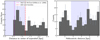 |
Fig. 19 Histograms of sensitivity filtered sources (see text) for the distance to the center of the supershell (left) and heliocentric distance of this subsample. The blue shaded area marks the distance range spanned by the shell. |
6 Summary and outlook
In order to extend our previous studies of the ISM and star formation (König et al. 2017; Urquhart et al. 2018) to the outer Galaxy between 225° ≤ ℓ ≤ 260°, we used Herschel/Hi-GAL 250 μm SPIRE continuum emission maps to select a representative sample of more than 800 sources from a rudimentary source catalog of more than 25 000 extracted clumps using SExtracor (Bertin & Arnouts 1996), giving positions and source sizes for these clumps.
We observed these sources in 12CO(2–1), identifying 1248 clouds that consist of a total of 1383 individual velocity components, for a total of 1090 positions, including recovered off-positions. Moreover, 966 (88.6%) lines of sight were found with a single velocity component, whereas two or more clouds were found toward 87 (11.4%) lines of sight, yielding on average 1.2 clouds each. Distances were calculated consecutively, using a rotation model of the Galaxy and applying the rotation curve from Brand & Blitz (1993) for all clouds and velocity components. For every line of sight, we finally associated the cloud with the highest integrated intensity to the corresponding dust clump. Combining our velocity measurements with H I emission maps from the GASS survey (McClure-Griffiths et al. 2004) and CO(1–0) maps from Dame et al. (2001), we were able investigate the large-scale structures of the southern outer Galaxy between 225° ≤ ℓ ≤ 260°.
We determined physical properties of the selected dust clumps, recovering their dust spectral energy distributions from Hi-GAL, MSX, and WISE continuum emission maps. The SEDs were consecutively fit with a simple two-component model yielding dust temperatures, integrated fluxes, and H2 column densities. Combining the results with the kinematic distances determined from the CO emission allows us to calculate physical properties such as bolometric luminosities and clump masses.
To guarantee the consistency of our data with other studies, we compare the peak H2 column densities obtained from dust continuum emission against the column density derived from the 12CO(2–1) emission. Although deviations of up to an order of magnitude are found for individual clumps, we find a good agreement for the general trend, and we allot the deviations to local variations in the gas-to-dust ratio and CO-to-H2 conversion factor. Furthermore, we compare the clump masses of our sample to a similar sample from Elia et al. (2013), finding the mean values to be almost identical and showing our methods to be reliable.
Our main findings are as follows:
- (i)
In general, we find the positions of the identified CO clouds to be strongly correlated with the highest column density parts of the H I emission. On the other hand, we were also able to identify a web of bridges, spurs, and blobs of star forming regions spanning between the larger star forming regions, unveiling the complex three-dimensional structure of the outer Galaxy in unprecedented detail. Although the latter might be an indication of the outer Galaxy being of a flucculent nature, a definite answer is difficult due to the influence of a large, expanding supershell (GSH242-03+37) in the survey area.
- (ii)
For the investigated clumps, we find the evolutionary stages to be well separated by the dust temperature, bolometric luminosity, and luminosity-to-mass ratio, which is consistent with our results in König et al. (2017). However, we find the clump masses and peak column densities to be similar in the starless and protostellar phase, but we find these quantities to be significantly higher for the YSO phase, indicating that the more massive clumps evolve significantly faster than their lower mass counterparts.
- (iii)
For the outer Galaxy, we find only 24 sources with an inferred luminosity higher than that of an early B-Type star (~ 8M⊙ Mottram et al. 2011), the masses of only eight sources above the threshold where it would be likely to host a massive dense core or high-mass protostar according to Csengeri et al. (2014), or at most 40 sources above the threshold for high-mass star formation as determined by Kauffmann et al. (2010). Even more so, we only find two methanol Class II masers; and ten known, as well as 24 candidate H II regions in the whole survey area of the outer Galaxy, indicating only a low fraction of star forming regions in the outer Galaxy capable of forming high-mass stars.
- (iv)
Investigating the influence of the expanding Galactic supershell GSH 242–03+37 in detail, we find the physical properties and star formation activity of sources located within the walls not to be statistically different from sources located farther away. Nevertheless, as we discuss in Sect. 5.3, we find the number density of sources increased within the walls of the supershell, leading us to the conclusion that the expanding supershell supports the formation of clumps, but once they collapse has no further influence.
In Paper II, we will use the sample of star forming regions characterized in the present work in order to compare the properties of the outer Galaxy with those found for the inner Galaxy, and thus derive global trends for the Milky Way.
Acknowledgements
This research made use of Astropy (http://www.astropy.org), a community-developed core Python package for Astronomy (Astropy Collaboration 2013) and the Astropy affilate software package photutils (https://github.com/astropy/photutils). This research made use of Montage, funded by the National Aeronautics and Space Administration’s Earth Science Technology Office, Computation Technologies Project, under Cooperative Agreement Number NCC5-626 between NASA and the California Institute of Technology. Montage is maintained by the NASA/IPAC Infrared Science Archive. This publication also makes use of data products from the Wide-field Infrared Survey Explorer, which is a joint project of the University of California, Los Angeles, and the Jet Propulsion Laboratory/California Institute of Technology, funded by the National Aeronautics and Space Administration.
References
- Anderson, L. D., Bania, T. M., Balser, D. S., et al. 2014, ApJS, 212, 1 [NASA ADS] [CrossRef] [Google Scholar]
- Astropy Collaboration (Robitaille, T. P., et al.) 2013, A&A, 558, A33 [NASA ADS] [CrossRef] [EDP Sciences] [Google Scholar]
- Benjamin, R. A., Churchwell, E., Babler, B. L., et al. 2005, ApJ, 630, L149 [NASA ADS] [CrossRef] [Google Scholar]
- Bertin, E., & Arnouts, S. 1996, A&AS, 117, 393 [NASA ADS] [CrossRef] [EDP Sciences] [Google Scholar]
- Bloemen, J. B. G. M., Bennett, K., Bignami, G. F., et al. 1984, A&A, 135, 12 [NASA ADS] [Google Scholar]
- Boomsma, R., Oosterloo, T. A., Fraternali, F., van der Hulst, J. M., & Sancisi, R. 2008, A&A, 490, 555 [NASA ADS] [CrossRef] [EDP Sciences] [Google Scholar]
- Brand, J., & Blitz, L. 1993, A&A, 275, 67 [NASA ADS] [Google Scholar]
- Brand, J., & Wouterloot, J. G. A. 1995, A&A, 303, 851 [NASA ADS] [Google Scholar]
- Contreras, Y., Schuller, F., Urquhart, J. S., et al. 2013, A&A, 549, A45 [NASA ADS] [CrossRef] [EDP Sciences] [Google Scholar]
- Csengeri, T., Urquhart, J. S., Schuller, F., et al. 2014, A&A, 565, A75 [NASA ADS] [CrossRef] [EDP Sciences] [Google Scholar]
- Dame, T. M., Elmegreen, B. G., Cohen, R. S., & Thaddeus, P. 1986, ApJ, 305, 892 [NASA ADS] [CrossRef] [Google Scholar]
- Dame, T. M., Hartmann, D., & Thaddeus, P. 2001, ApJ, 547, 792 [NASA ADS] [CrossRef] [Google Scholar]
- Dobbs, C., & Baba, J. 2014, PASA, 31, e035 [NASA ADS] [CrossRef] [Google Scholar]
- Eden, D. J., Moore, T. J. T., Morgan, L. K., Thompson, M. A., & Urquhart, J. S. 2013, MNRAS, 431, 1587 [NASA ADS] [CrossRef] [Google Scholar]
- Eden, D. J., Moore, T. J. T., Urquhart, J. S., et al. 2015, MNRAS, 452, 289 [NASA ADS] [CrossRef] [Google Scholar]
- Elia, D., Molinari, S., Fukui, Y., et al. 2013, ApJ, 772, 45 [NASA ADS] [CrossRef] [Google Scholar]
- Elia, D., Molinari, S., Schisano, E., et al. 2017, MNRAS, 471, 100 [NASA ADS] [CrossRef] [Google Scholar]
- Galyardt, J., & Shelton, R. L. 2016, ApJ, 816, L18 [CrossRef] [Google Scholar]
- García, P., Bronfman, L., Nyman, L.-Å., Dame, T. M., & Luna, A. 2014, ApJS, 212, 2 [NASA ADS] [CrossRef] [Google Scholar]
- Giannetti, A., Leurini, S., König, C., et al. 2017a, A&A, 606, L12 [NASA ADS] [CrossRef] [EDP Sciences] [Google Scholar]
- Giannetti, A., Leurini, S., Wyrowski, F., et al. 2017b, A&A, 603, A33 [NASA ADS] [CrossRef] [EDP Sciences] [Google Scholar]
- Green, J. A., Caswell, J. L., Fuller, G. A., et al. 2012, MNRAS, 420, 3108 [NASA ADS] [CrossRef] [Google Scholar]
- Griffin, M. J., Abergel, A., Abreu, A., et al. 2010, A&A, 518, L3 [EDP Sciences] [Google Scholar]
- Güsten, R., Nyman, L. Å., Schilke, P., et al. 2006, A&A, 454, L13 [NASA ADS] [CrossRef] [EDP Sciences] [Google Scholar]
- Heiles, C. 1979, ApJ, 229, 533 [NASA ADS] [CrossRef] [Google Scholar]
- Heyer, M., & Dame, T. M. 2015, ARA&A, 53, 583 [NASA ADS] [CrossRef] [Google Scholar]
- Heyer, M. H., Carpenter, J. M., & Snell, R. L. 2001, ApJ, 551, 852 [NASA ADS] [CrossRef] [Google Scholar]
- Izumi, N., Kobayashi, N., Yasui, C., et al. 2014, ApJ, 795, 66 [CrossRef] [Google Scholar]
- Kauffmann, J., Bertoldi, F., Bourke, T. L., Evans, II, N. J., & Lee, C. W. 2008, A&A, 487, 993 [NASA ADS] [CrossRef] [EDP Sciences] [Google Scholar]
- Kauffmann, J., Pillai, T., Shetty, R., Myers, P. C., & Goodman, A. A. 2010, ApJ, 716, 433 [NASA ADS] [CrossRef] [Google Scholar]
- Kennicutt, R. C. 2005, IAU Symp., 227, 3 [NASA ADS] [CrossRef] [Google Scholar]
- Kim, B. G., Kawamura, A., Yonekura, Y., & Fukui, Y. 2004, PASJ, 56, 313 [NASA ADS] [Google Scholar]
- Klein, B., Hochgürtel, S., Krämer, I., et al. 2012, A&A, 542, L3 [NASA ADS] [CrossRef] [EDP Sciences] [Google Scholar]
- Kobayashi, N., Yasui, C., Tokunaga, A. T., & Saito, M. 2008, ApJ, 683, 178 [NASA ADS] [CrossRef] [Google Scholar]
- Koda, J., Scoville, N., & Heyer, M. 2016, ApJ, 823, 76 [NASA ADS] [CrossRef] [Google Scholar]
- König, C., Urquhart, J. S., Csengeri, T., et al. 2017, A&A, 599, A139 [NASA ADS] [CrossRef] [EDP Sciences] [Google Scholar]
- Koo, J.-R., Lee, J. W., & Hong, K. 2017, AJ, 154, 235 [CrossRef] [Google Scholar]
- Lemasle, B., Hajdu, G., Kovtyukh, V., et al. 2018, A&A, 618, A160 [NASA ADS] [CrossRef] [EDP Sciences] [Google Scholar]
- Lumsden, S. L., Hoare, M. G., Urquhart, J. S., et al. 2013, ApJS, 208, 11 [NASA ADS] [CrossRef] [Google Scholar]
- May, J., Alvarez, H., & Bronfman, L. 1997, A&A, 327, 325 [NASA ADS] [Google Scholar]
- McClure-Griffiths, N. M., Dickey, J. M., Gaensler, B. M., & Green, A. J. 2004, ApJ, 607, L127 [NASA ADS] [CrossRef] [Google Scholar]
- McClure-Griffiths, N. M., Dickey, J. M., Gaensler, B. M., Green, A. J., & Haverkorn, M. 2006, ApJ, 652, 1339 [NASA ADS] [CrossRef] [Google Scholar]
- McClure-Griffiths, N. M., Pisano, D. J., Calabretta, M. R., et al. 2009, ApJS, 181, 398 [NASA ADS] [CrossRef] [Google Scholar]
- Miville-Deschênes, M.-A., Murray, N., & Lee, E. J. 2017, ApJ, 834, 57 [NASA ADS] [CrossRef] [Google Scholar]
- Molinari, S., Pezzuto, S., Cesaroni, R., et al. 2008, A&A, 481, 345 [NASA ADS] [CrossRef] [EDP Sciences] [Google Scholar]
- Molinari, S., Swinyard, B., Bally, J., et al. 2010, PASP, 122, 314 [NASA ADS] [CrossRef] [Google Scholar]
- Molinari, S., Schisano, E., Elia, D., et al. 2016, A&A, 591, A149 [NASA ADS] [CrossRef] [EDP Sciences] [Google Scholar]
- Mooney, T. J., & Solomon, P. M. 1988, ApJ, 334, L51 [NASA ADS] [CrossRef] [Google Scholar]
- Mottram, J. C., Hoare, M. G., Davies, B., et al. 2011, ApJ, 730, L33 [NASA ADS] [CrossRef] [Google Scholar]
- Nakagawa, M., Onishi, T., Mizuno, A., & Fukui, Y. 2005, PASJ, 57, 917 [NASA ADS] [Google Scholar]
- Ossenkopf, V., & Henning, T. 1994, A&A, 291, 943 [NASA ADS] [Google Scholar]
- Park, G., Koo, B.-C., Kang, J.-h., et al. 2016, ApJ, 827, L27 [NASA ADS] [CrossRef] [Google Scholar]
- Planck Collaboration Int. XIX. 2015, A&A, 576, A104 [NASA ADS] [CrossRef] [EDP Sciences] [Google Scholar]
- Poglitsch, A., Waelkens, C., Geis, N., et al. 2010, A&A, 518, L2 [NASA ADS] [CrossRef] [EDP Sciences] [Google Scholar]
- Price, S. D., Egan, M. P., Carey, S. J., Mizuno, D. R., & Kuchar, T. A. 2001, AJ, 121, 2819 [NASA ADS] [CrossRef] [Google Scholar]
- Reid, M. J., Menten, K. M., Brunthaler, A., et al. 2014, ApJ, 783, 130 [Google Scholar]
- Reid, M. J., Dame, T. M., Menten, K. M., & Brunthaler, A. 2016, ApJ, 823, 77 [NASA ADS] [CrossRef] [Google Scholar]
- Reid, M. J., Menten, K. M., Brunthaler, A., et al. 2019, ApJ, 885, 131 [NASA ADS] [CrossRef] [Google Scholar]
- Rice, T. S., Goodman, A. A., Bergin, E. A., Beaumont, C., & Dame, T. M. 2016, ApJ, 822, 52 [NASA ADS] [CrossRef] [Google Scholar]
- Roman-Duval, J., Jackson, J. M., Heyer, M., et al. 2009, ApJ, 699, 1153 [NASA ADS] [CrossRef] [Google Scholar]
- Rudolph, A. L., Simpson, J. P., Haas, M. R., Erickson, E. F., & Fich, M. 1997, ApJ, 489, 94 [NASA ADS] [CrossRef] [Google Scholar]
- Sandstrom, K. M., Leroy, A. K., Walter, F., et al. 2013, ApJ, 777, 5 [NASA ADS] [CrossRef] [Google Scholar]
- Schulman, E. 1996, PASP, 108, 460 [CrossRef] [Google Scholar]
- Solomon, P. M., Rivolo, A. R., Barrett, J., & Yahil, A. 1987, ApJ, 319, 730 [NASA ADS] [CrossRef] [Google Scholar]
- Urquhart, J. S., Csengeri, T., Wyrowski, F., et al. 2014a, A&A, 568, A41 [NASA ADS] [CrossRef] [EDP Sciences] [Google Scholar]
- Urquhart, J. S., Figura, C. C., Moore, T. J. T., et al. 2014b, MNRAS, 437, 1791 [NASA ADS] [CrossRef] [Google Scholar]
- Urquhart, J. S., Moore, T. J. T., Csengeri, T., et al. 2014c, MNRAS, 443, 1555 [NASA ADS] [CrossRef] [Google Scholar]
- Urquhart, J. S., Moore, T. J. T., Menten, K. M., et al. 2015, MNRAS, 446, 3461 [NASA ADS] [CrossRef] [Google Scholar]
- Urquhart, J. S., König, C., Giannetti, A., et al. 2018, MNRAS, 473, 1059 [NASA ADS] [CrossRef] [Google Scholar]
- Vallée, J. P. 2015, MNRAS, 450, 4277 [CrossRef] [Google Scholar]
- Vassilev, V., Meledin, D., Lapkin, I., et al. 2008, A&A, 490, 1157 [NASA ADS] [CrossRef] [EDP Sciences] [Google Scholar]
- Wienen, M., Wyrowski, F., Menten, K. M., et al. 2015, A&A, 579, A91 [NASA ADS] [CrossRef] [EDP Sciences] [Google Scholar]
- Woltjer, L. 1974, Astrophys. Space Sci. Lib., 45, 323 [CrossRef] [Google Scholar]
- Wouterloot, J. G. A., & Brand, J. 1989, A&AS, 80, 149 [NASA ADS] [Google Scholar]
- Wright, E. L., Eisenhardt, P. R. M., Mainzer, A. K., et al. 2010, AJ, 140, 1868 [Google Scholar]
GILDAS/CLASS: https://www.iram.fr/IRAMFR/GILDAS/
Within 15, 10, 7, or 5 min, for PWV < 1.5, < 3, < 4, ≥ 4 mm, assuming increasing weather stability with lower PWV.
F20 is the flux in the 21 μm or 22 μm band from either MSX or WISE.
The ATLASGAL Top100 sample (König et al. 2017) defines a sample of the ≈ 100 brightest sources in four distinct evolutionary stages selected from the ATLASGAL survey.
The broad peak between 1.4 and 3.2 kpc in Fig. 18 is not associated with the shell, but the superposition of different clusters of clumps in the observed region.
All Tables
Astrometric data and integrated flux as determined by SExtractor for the extracted clumps for the first 20 clumps from a total of 23 817 sources.
Overview of the six dominating bright and complex regions and the number of sources taken into account in the present paper.
Velocity components identified from the CO(2–1) observations along ten lines of sight.
Clouds (i.e., coherent groups of velocity components) identified from the CO(2–1) observations along a given line of sight for 15 complexes.
Summary of physical properties of the whole population of clumps and the three evolutionary subsamples identified.
All Figures
|
Fig. 1 Imageof SPIRE 250 μm emission showing an example of extracted sources around ℓ = 236° and b = − 1°. The image spans ~7° in longitude and ~3° in latitude. Overplotted are the sources identified by SExtractor (green ellipses). |
| In the text | |
|
Fig. 2 Red-green-blue (RGB) images of the six brightest regions in the survey area. These have been excluded from the automated source selection to avoid biasing the survey toward these regions. Red: SPIRE 500 μm; Green: SPIRE 250 μm; Blue: PACS70 μm. |
| In the text | |
|
Fig. 3 Histogram showing integrated flux for the sources identified by SExtractor (gray) in comparison with those selected for our observations (blue) and those recovered from contaminated off-source positions (green; see Sect. 2.3). The red vertical dashed line indicates the limit of ~2.5 Jy that was imposed as a selection threshold (see text for details). |
| In the text | |
|
Fig. 4 12CO(2–1) spectra (black line) showing different typical profiles: single component (upper left), multiple components (upper right), simple contamination in the off-position (lower left), and a complex spectrum with all features (lower right). The total fit spectrum is overplotted in blue. Coherent velocity complexes are either marked as black (source position) or red (off position; negative features) horizontal bars below the spectrum. The vertical dashed blue lines indicate the peak positions of the fit Gaussian profiles, whereas the vertical red dashed lines indicate the peak position of the emission found in theoff-position. |
| In the text | |
|
Fig. 5 Galactic longitude versus radial velocity. The dots mark all clouds found above 5σ rms between 260° ≤ ℓ ≤ 225°, with the peak antenna temperature color-coded. Background image: CO(1–0) emission from Dame et al. (2001). Dashed yellow, magenta, and green lines: peaks at 9, 11, and 14.0 kpc, respectively, as found in Fig. 7. The spiral arms and the position of the local emission as determined from H I emission are marked by the colored solid lines. Cyan: local emission; green: Perseus arm; red: outer arm. The solid magenta ellipse marks the rim of the Galactic supershell GSH 242-3+77. Gray dashed lines: galactocentric radii at 10 and 15 kpc. The green stars mark the positions of the three sources from the Methanol Multibeam (MMB; Green et al. 2012) survey found in the region. |
| In the text | |
|
Fig. 6 Third quadrant of the Milky Way. The dots mark all clouds above 5σ rms, using the same color-coding as Fig. 5. The observed region (225° < ℓ < 260°) is highlighted in light blue. Heliocentric distances d and galactocentric radii R are indicated as dash-dotted black and dotted gray circles, respectively. Positions of arms and local emission are indicated by solid lines in the same colors as in Fig. 5. The position of the Galactic supershell GSH 242-3+37 is indicated by the magenta ellipse. From the observed vlsr we calculated the heliocentric distances for each cloud using the Brand & Blitz (1993) rotation curve to obtain Galactic positions. |
| In the text | |
|
Fig. 7 Histograms showing CO velocity components above 5σ (light gray), CO emission groups/clouds (dark gray) and matched dust clumps (black outline) by galactocentric (upper) and heliocentric (lower) distance. The vertical dashed yellow line indicates the peak associated with local emission. The magenta and green shaded areas mark the distance range between 225° ≤ ℓ≤ 260° of theloci of the Perseus and Outer arms, respectively. The two peaks between rgal ~ 12 and ~ 13 kpc correspond to complexes between the Perseus and Outer arm. |
| In the text | |
|
Fig. 8 Sample SED (G253.29-1.61) with hot and cold components, classifying this source as a young stellar object (YSO). |
| In the text | |
|
Fig. 9 Consistency checks. Top: comparing peak N |
| In the text | |
|
Fig. 10 Observational distance biases. Bolometric luminosity (top), clump mass (middle), and linear source size (bottom) versus heliocentric distance. The solid lines mark the distance-dependent sensitivity/resolution limit. The horizontally dashed green lines mark the limit above which our survey does not suffer from a distance bias up to 9 kpc (vertical dotted line). |
| In the text | |
|
Fig. 11 Cumulative distributions for derived parameters of this survey. Colored lines indicate the distribution for the different evolutionary phases, whereas the dark gray line represents the full sample. |
| In the text | |
|
Fig. 12 Bolometric luminosity versus clump mass. The gray tracks indicate the evolutionary path through the diagram for the given initial masses as calculated by Molinari et al. (2008). The diagonal solid line marks the expected luminosity for a given mass for a zero-age main-sequence (ZAMS) star. The horizontal dashed line indicates the expected luminosity for a B2 star (~ 8M⊙) as calculated by Mottram et al. (2011). The vertical dashed line marks the threshold calculated by Csengeri et al. (2014) above whichthe clumps are likely to host massive dense cores or a high-mass protostar. The dash-dotted lines are linear fits to the three evolutionary classes. |
| In the text | |
|
Fig. 13 Clump mass versus source radius. The shaded area marks the regime where only low-mass stars form, as determined by Kauffmann et al. (2010). The black dashed line marks the lower limit for effective high-mass star formation as determined by Urquhart et al. (2014c), indicating a surface density threshold of 0.05 g cm−2. The horizontal gray dotted line marks the threshold of 8 M⊙, above whicha clump is considered massive. The colored dash-dotted lines are linear fits to the corresponding subsamples, and the cyan dash-dotted line is a fit to the full sample. |
| In the text | |
|
Fig. 14 HI emission from the Galactic All Sky HI Survey (GASS; McClure-Griffiths et al. 2009) for a larger region of the outer Galaxy covering 215° < ℓ < 280° indicating the integrated brightness temperature between − 5° < b < 1.5°. Overplottedare the positions of the spiral arms from Reid et al. (2014, 2019), and Vallée (2015) as dashed, dotted, and dash-dotted lines, respectively. The spiral arms and local emission as determined in the present work are marked by the solid lines. The dotted gray lines mark galactocentric radii at 10 and 15 kpc. the solid magenta ellipse marks the position of the Galactic supershell GSH 242-3+37. The light blue area framed by the blue dotted lines marks the area of the present work. |
| In the text | |
|
Fig. 15 Galactic longitude versus radial velocity integrated for slices of Galactic latitude. Latitude ranges from b = + 0.5° (top left panel) to b = −3.0° (lower right panel). Crosses mark the CO(2–1) velocity components along a line-of-sight, with colored dots indicating associated dust clumps. Sizes correspond to the integrated line intensity and the colors for the dust clumps to the 22 μm WISE emission being indicative of ongoing star formation. The background image shows the corresponding H I integrated intensity from the GASS survey (McClure-Griffiths et al. 2004). The contours mark the CO(1–0) emission from Dame et al. (2001) at levels of 3σ, 5σ, 7σ and the 10th, 30th, 50th and 70th percentile. The spiral arms as determined in the present work and the position of the local emission are marked by the colored solid lines. Cyan: local emission; green: Perseus arm; red: outer arm. The solid magenta ellipse marks the position of the Galactic supershell GSH 242-3+37. |
| In the text | |
|
Fig. 16 Selected slices of Galactic latitude versus radial velocity integrated over 3° in Galactic longitude away from the Galactic supershell (top: higher longitudes than shell, bottom: lower longitudes of the shell). Crosses mark the CO(2–1) velocity components along a line of sight, with colored dots indicating associated dust clumps. Sizes correspond to the integrated line intensity and the colors reflect ongoing star formation as indicated by the 22 μm WISE emission. The background image shows the corresponding H I integrated intensity from the GASS survey (McClure-Griffiths et al. 2004). The contours mark the CO(1–0) emission from Dame et al. (2001) at levels of 5σ, 7σ, and the 10th, 30th, 50th and 70th percentiles. The spiral arms as determined in the present work and the position of the local emission are marked by the colored solid lines. Cyan: local emission; green: Perseus arm; red: outer arm. |
| In the text | |
|
Fig. 17 Slices of Galactic latitude versus radial velocity integrated over 3° in Galactic longitude at the edges (top, bottom) and the center (middle) of the Galactic supershell. Colored dots mark the positions of the dust clumps, and white crosses mark the positions of clouds identified by the CO(2–1) pointed observations that are not associated with the dust clump. The background image shows the corresponding H I integrated intensity from the GASS survey (McClure-Griffiths et al. 2004). The contours mark the CO(1–0) emission from Dame et al. (2001) at levels of 5σ, 7σ, and the 10th, 30th, 50th and 70th percentiles. The spiral arms as determined in the present work and the position of the local emission are marked by the colored solid lines. Cyan: local emission; green: Perseus arm; red: outer arm. |
| In the text | |
|
Fig. 18 Histogram for distance of all clouds identified in CO to the center of the supershell. The edge of the supershell is clearly distinguishable from the other sources, with the central parts at R < 0.4 kpc being void of any CO clouds. |
| In the text | |
|
Fig. 19 Histograms of sensitivity filtered sources (see text) for the distance to the center of the supershell (left) and heliocentric distance of this subsample. The blue shaded area marks the distance range spanned by the shell. |
| In the text | |
Current usage metrics show cumulative count of Article Views (full-text article views including HTML views, PDF and ePub downloads, according to the available data) and Abstracts Views on Vision4Press platform.
Data correspond to usage on the plateform after 2015. The current usage metrics is available 48-96 hours after online publication and is updated daily on week days.
Initial download of the metrics may take a while.