| Issue |
A&A
Volume 645, January 2021
|
|
|---|---|---|
| Article Number | A67 | |
| Number of page(s) | 22 | |
| Section | Stellar structure and evolution | |
| DOI | https://doi.org/10.1051/0004-6361/202039337 | |
| Published online | 13 January 2021 | |
Spectroscopic evolution of massive stars near the main sequence at low metallicity⋆
LUPM, Université de Montpellier, CNRS, Place Eugène Bataillon, 34095 Montpellier, France
e-mail: This email address is being protected from spambots. You need JavaScript enabled to view it.
Received:
3
September
2020
Accepted:
16
October
2020
Abstract
Context. The evolution of massive stars is not fully understood. Several physical processes affect their life and death, with major consequences on the progenitors of core-collapse supernovae, long-soft gamma-ray bursts, and compact-object mergers leading to gravitational wave emission.
Aims. In this context, our aim is to make the prediction of stellar evolution easily comparable to observations. To this end, we developed an approach called “spectroscopic evolution” in which we predict the spectral appearance of massive stars through their evolution. The final goal is to constrain the physical processes governing the evolution of the most massive stars. In particular, we want to test the effects of metallicity.
Methods. Following our initial study, which focused on solar metallicity, we investigated the low Z regime. We chose two representative metallicities: 1/5 and 1/30 Z⊙. We computed single-star evolutionary tracks with the code STAREVOL for stars with initial masses between 15 and 150 M⊙. We did not include rotation, and focused on the main sequence (MS) and the earliest post-MS evolution. We subsequently computed atmosphere models and synthetic spectra along those tracks. We assigned a spectral type and luminosity class to each synthetic spectrum as if it were an observed spectrum.
Results. We predict that the most massive stars all start their evolution as O2 dwarfs at sub-solar metallicities contrary to solar metallicity calculations and observations. The fraction of lifetime spent in the O2V phase increases at lower metallicity. The distribution of dwarfs and giants we predict in the SMC accurately reproduces the observations. Supergiants appear at slightly higher effective temperatures than we predict. More massive stars enter the giant and supergiant phases closer to the zero-age main sequence, but not as close as for solar metallicity. This is due to the reduced stellar winds at lower metallicity. Our models with masses higher than ∼60 M⊙ should appear as O and B stars, whereas these objects are not observed, confirming a trend reported in the recent literature. At Z = 1/30 Z⊙, dwarfs cover a wider fraction of the MS and giants and supergiants appear at lower effective temperatures than at Z = 1/5 Z⊙. The UV spectra of these low-metallicity stars have only weak P Cygni profiles. He II 1640 sometimes shows a net emission in the most massive models, with an equivalent width reaching ∼1.2 Å. For both sets of metallicities, we provide synthetic spectroscopy in the wavelength range 4500−8000 Å. This range will be covered by the instruments HARMONI and MOSAICS on the Extremely Large Telescope and will be relevant to identify hot massive stars in Local Group galaxies with low extinction. We suggest the use of the ratio of He I 7065 to He II 5412 as a diagnostic for spectral type. Using archival spectroscopic data and our synthetic spectroscopy, we show that this ratio does not depend on metallicity. Finally, we discuss the ionizing fluxes of our models. The relation between the hydrogen ionizing flux per unit area versus effective temperature depends only weakly on metallicity. The ratios of He I and He II to H ionizing fluxes both depend on metallicity, although in a slightly different way.
Conclusions. We make our synthetic spectra and spectral energy distributions available to the community.
Key words: stars: massive / stars: atmospheres / techniques: spectroscopic / stars: evolution / stars: early-type
Pollux database is also available at the CDS via anonymous ftp to cdsarc.u-strasbg.fr (130.79.128.5) or via http://cdsarc.u-strasbg.fr/viz-bin/cat/J/A+A/645/A67
© F. Martins and A. Palacios 2021
 Open Access article, published by EDP Sciences, under the terms of the Creative Commons Attribution License (https://creativecommons.org/licenses/by/4.0), which permits unrestricted use, distribution, and reproduction in any medium, provided the original work is properly cited.
1. Introduction
Understanding the evolution and final fate of massive stars is of primordial importance now that observations of core-collapse supernovae, long-soft gamma-ray bursts (LGRBs), and compact-object mergers are becoming almost routine. However, many uncertainties still hamper unambiguous predictions from evolutionary models (e.g., Martins & Palacios 2013). Although mass loss (Chiosi & Maeder 1986) and rotation (Maeder & Meynet 2000) have long been recognized as key drivers of stellar evolution, other processes significantly affect the way massive stars evolve. Magnetism, which is present at the surface of a minority of OB stars (Grunhut et al. 2017), may strongly impact the outcome of their evolution (Keszthelyi et al. 2019). An uncertain but potentially large fraction of massive stars have a companion that will modify the properties of the star compared to isolation (e.g., Moe & Di Stefano 2013; Kobulnicky et al. 2014; de Mink et al. 2013; Mahy et al. 2020).
Metallicity is another major driver of the evolution of massive stars. It modifies opacities and therefore the internal structure of stars. As a result, massive metal-poor stars are usually hotter and more compact (Maeder & Meynet 2001). The resulting steeper gradients are predicted to enhance the effects of rotation on stellar evolution (Maeder & Meynet 2000), although direct observational confirmation is still lacking. At lower metallicity, radiatively driven winds are weaker (Vink et al. 2001; Mokiem et al. 2007a), meaning that the effects of mass loss are reduced. The binary fraction at low metallicity is not well constrained: Moe & Di Stefano (2013) find no differences between the Magellanic Clouds and the Galaxy, while Dorn-Wallenstein & Levesque (2018) report a possible decrease of the binary fraction at lower metallicity among high-mass stars, in contrast to what is observed for low-mass stars (Raghavan et al. 2010). Stanway et al. (2020) studied how the uncertainties in binary parameters affect the global predictions of population-synthesis models. These latter authors concluded that varying the binary properties for high-mass stars leads to variations that do not exceed those caused by metallicity. The metallicity effects on rotation and mass loss also impact the occurrence of LGRBs. Japelj et al. (2018) and Palmerio et al. (2019) show that low metallicity is favored for LGRBs, and there is a metallicity threshold above which they are seldom observed (Vergani et al. 2015; Perley et al. 2016). Metallicity therefore appears to be a major ingredient of massive star evolution.
In the present paper, we discuss the role of metallicity in the spectroscopic appearance of massive stars on and close to the main sequence (MS). This extends the work we presented in Martins & Palacios (2017) in which we described our method to produce spectroscopic sequences along evolutionary tracks. This method consists in computing atmosphere models and synthetic spectra at dedicated points sampling an evolutionary track, and was pioneered by Schaerer et al. (1996) and recently revisited by us and Groh et al. (2013, 2014). Götberg et al. (2017, 2018) used a similar approach to investigate the ionizing properties of stars stripped of their envelope in binary systems. These latter authors found that such objects emit a large number of ionizing photons, equivalent to Wolf-Rayet stars. Kubátová et al. (2019) looked at the spectral appearance of stars undergoing quasi-chemically homogeneous evolution (Maeder 1987; Yoon et al. 2006), focusing on metal-poor objects (Z = 1/50 Z⊙), for this type of evolution seems to be more easily achieved at that metallicity (e.g., Brott et al. 2011). Kubátová et al. (2019) concluded that for most of their evolution, which proceeds directly leftward of the zero age main sequence (ZAMS), stars show only absorption lines in their synthetic spectra, therefore appearing as early-type O stars. In the present work, similarly to Martins & Palacios (2017), we focus on the MS and early post-MS evolution because these phases are the least affected by uncertainties (see Martins & Palacios 2013). Our goal is to predict the spectral properties of stars at low metallicity, to compare them with observational data, and ultimately to provide constraints on stellar evolution. To this end, we selected two representative metallicities: 1/5 Z⊙ and 1/30 Z⊙. The former is the classical value of the Small Magellanic Cloud (SMC), and the latter is on the low side of the distribution of metallicities in Local Group dwarf galaxies (McConnachie et al. 2005; Ross et al. 2015). These two values of metallicity should therefore reasonably bracket the metal content of most stars that will be observed individually in the Local Group with next-generation telescopes such as the Extremely Large Telescope (ELT). In preparation for these future observations, we make predictions on the spectral appearance of hot massive stars in these metal-poor environments. We also provide classification criteria suitable for the ELT instruments.
In Sect. 2 we describe our method. We present our spectroscopic sequences in Sect. 3, where we also define a new spectral type diagnostic. We present the ionizing properties of our models in Sect. 4. In this section we also discuss He II 1640 emission that is present in some of our models. Finally, we conclude in Sect. 5.
2. Method
2.1. Evolutionary models and synthetic spectra
We computed evolutionary models for massive stars with the code STAREVOL (Decressin et al. 2009; Amard et al. 2016). We assumed an Eddington grey atmosphere as outer boundary condition to the stellar structure equations. We used the Asplund et al. (2009) solar chemical composition as a reference, with Z⊙ = 0.0134. A calibration of the solar model with the present input physics leads to an initial helium mass fraction Y = 0.2689 at solar metallicity. We used the corresponding constant slope ΔY/ΔZ = 1.60 (with the primordial abundance Y0 = 0.2463 based on WMAP-SBBN by Coc et al. 2004) to compute the initial helium mass fraction at Z = 2.69 × 10−3 = 1/5 Z⊙ and Z = 4.48 × 10−4 = 1/30 Z⊙, and to scale all the abundances accordingly. The OPAL opacities used for these models comply to this scaled distribution of nuclides. We did not include specific α-element enhancement in our models. We described the convective instability using the mixing-length theory with αMLT = 1.6304, and we use the Schwarzschild instability criterion to define the boundaries of convective regions. We added a step overshoot at the convective core edge and adopt αov = 0.1Hp, with Hp being the pressure scale height. We used the thermonuclear reaction rates from the NACRE II compilation (Xu et al. 2013a) for mass number A < 16, and the ones from the NACRE compilation (Angulo et al. 1999) for more massive nuclei up to Ne. The proton captures on nuclei more massive than Ne are from Longland et al. (2010) or Iliadis et al. (2001). The network was generated via the NetGen server (Xu et al. 2013b).
We used the mass-loss-rate prescriptions of Vink et al. (2001), who account for the metallicity scaling of mass-loss rates (see also Mokiem et al. 2007a). In order to account for the effect of clumping in the wind (Fullerton 2011), the obtained mass-loss rates were divided by a factor of three (Cohen et al. 2014). This reduction is consistent with the revision of theoretical mass-loss rates proposed by Lucy (2010), Krtička & Kubát (2017), and Björklund et al. (2021).
Along each evolutionary sequence, we selected points for which we computed an atmosphere model and the associated synthetic spectrum with the code CMFGEN (Hillier & Miller 1998). CMFGEN solves the radiative transfer and statistical equilibrium equations under non-LTE conditions using a super-level approach. The temperature structure is set from the constraint of radiative equilibrium. A spherical geometry is adopted to account for stellar winds. The input velocity structure is a combination of a quasi-static equilibrium solution below the sonic point and a β-velocity law above it (i.e., v = v∞ × (1 − R/r)β, where v∞ is the maximal velocity at the top of the atmosphere and R is the stellar radius). We adopted v∞ = 3.0 × vesc as in Martins & Palacios (2017) 1. This value is consistent with both observations (Garcia et al. 2014) and theoretical predictions (Björklund et al. 2021) in which v∞/vesc is in the ranges 1.0−6.0 and 2.5−5.5, respectively. We note that the observational study of Garcia et al. (2014) shows a correlation between terminal velocity and metallicity (see also Leitherer et al. 1992), but no clear trend can be seen between the very scattered ratio v∞/vesc and metallicity. The velocity structure below the sonic point is iterated a few times during the atmosphere model calculation, taking the radiative force resulting from the radiation field and level populations into account. The density structure follows from the velocity structure and mass conservation equation. The models include the following elements: H, He, C, N, O, Ne, Mg, Si, S, Ar, Ca, Fe, and Ni. A total of about 7100 atomic levels2 and nearly 170 000 atomic transitions are taken into account. Once the atmosphere model is converged, a formal solution of the radiative transfer equation is performed and leads to the synthetic spectrum in the wavelength range 10 Å–50 μm. In that process, a depth-variable microturbulent velocity varying from 10 km s−1 at the bottom of the photosphere to 10% of the terminal velocity at the top of the atmosphere is adopted.
Figure 1 shows the Hertzsprung-Russell diagram at the two selected metallicities. The optical spectra and spectral energy distributions (SEDs) are distributed through the POLLUX3 database (Palacios et al. 2010). The parameters adopted for their computations are listed in Tables A.1 and A.2.
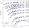 |
Fig. 1. Hertzsprung-Russell diagram for the Z = 1/30 Z⊙ (black lines and filled squares) and SMC (dot-dashed blue lines and open circles) cases. Lines are the STAREVOL evolutionary tracks. Symbols are the points at which an atmosphere model and synthetic spectrum have been computed. |
2.2. Spectral classification
Once the synthetic spectra were calculated, we performed a spectral classification as if they were results of observations. We followed the method presented by Martins & Palacios (2017) with some slight adjustments. Our process can be summarized as follows:
– Spectral type: The main classification criterion for O stars is the relative strength of He I 4471 and He II 4542 as proposed by Conti & Alschuler (1971) and quantified by Mathys (1988). For each spectrum, we therefore computed the equivalent width (EW) of both lines and calculated the logarithm of their ratio. A spectral type was assigned according to the Mathys scheme. For spectral types O9 to O9.7, we refined the classification using the criteria defined by Sota et al. (2011) and quantified by Martins (2018), namely  and
and  . For B stars, we estimated the relative strength of Si IV 4089 and Si III 4552. We used the atlas of Walborn & Fitzpatrick (1990) to assign B-type sub-classes. Finally, for the earliest O stars (O2 to O3.5) we relied on the relative strength of N III 4640 and N IV 4058 as defined by Walborn et al. (2002).
– Luminosity class: For O stars earlier than O8.5, the strength of He II 4686 was the main classification criterion. We used the quantitative scheme presented by Martins (2018) to assign luminosity classes. For stars with spectral type between O9 and O9.7, we used the ratio  defined by Sota et al. (2011) and quantified by Martins (2018). For B stars, we relied mainly on the morphology of Hγ which is broad in dwarfs and gets narrower in giants and supergiants.
For both spectral type and luminosity class assignment we discarded classification criteria based on the relative strengths of Si to He lines because they are metallicity dependent and this dependence is not quantified at metallicities different from solar.
For all stars, a final step in the classification process involved a direct comparison with standard stars. The spectra of these reference objects were retrieved from the GOSC catalog4 for O stars and from the POLARBASE archive5 for B stars. The final spectral classes and luminosity classes are given in Tables A.1 and A.2.
3. Spectroscopic sequences
In this section we discuss the spectroscopic sequences along the evolutionary tracks that we obtained. We first describe general trends before examining the two selected metallicities.
3.1. Example of spectroscopic sequences
We first describe full spectroscopic sequences for typical cases. In Fig. 2 we show the optical spectra computed along the 60 M⊙ tracks. According to our computations, the star appears as a O3−3.5 dwarf on the ZAMS and enters the post-MS evolution as a late-O/early-B supergiant. This is valid for both the SMC and one-thirtieth solar metallicities. The evolution of the He I 4471 to He II 4542 line ratio – the main spectral type classification criterion (Conti & Alschuler 1971) – is clearly seen. Figure 2 highlights the reduction of the metal lines at lower metallicity: for Z = 1/30 Z⊙, silicon, nitrogen, and carbon lines are weaker than for a SMC metallicity. When comparing to Fig. 6 of Martins & Palacios (2017) which shows solar metallicity computations, the effect is even more striking. This effect is magnified in the ultraviolet range. Figure 3 shows the spectroscopic sequences for the same 60 M⊙ tracks, but between 1200 and 1900 Å. First, the strong P Cygni lines are severely reduced in the one-thirtieth solar metallicity spectra. This is due to the reduction in both mass-loss rate and metal abundance. Second, the iron photospheric lines are weaker in the lower metallicity spectra. Figure 3 illustrates the change of iron ionization when Teff varies: at early spectral types, and therefore high Teff, Fe V lines dominate the absorption spectrum around 1400 Å; at late spectral types, it is Fe IV lines and even Fe III lines in the coolest cases that are stronger.
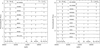 |
Fig. 2. Optical spectra of the sequence of models calculated along the 60 M⊙ track at SMC (left) and one-thirtieth (right) metallicity from the ZAMS at the top to the post-MS at the bottom. The main diagnostic lines are indicated at the bottom of the figure. The spectra have been degraded to a spectral resolution of ∼2500, similar to that of the GOSS survey. |
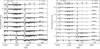 |
Fig. 3. Same as Fig. 2 but for the UV range. The spectra have been degraded to a spectral resolution of ∼16 000 typical of HST/COS FUV observations. |
Figures B.1 and B.2 show the optical and UV sequences followed by a 20 M⊙ star. Qualitatively, the trends are the same as for the 60 M⊙ star. Figure B.3 displays the sequences of the 60 M⊙ stars in the K-band. At these wavelengths, the number of lines is reduced and there are very few metallic lines. The effects of metallicity are therefore difficult to identify. The C IV lines around 2.06−2.08 μm almost disappear at Z = 1/30 Z⊙. The N III/O III emission complex near 2.11 μm is also reduced. These figures illustrate that the K-band is far from being an optimal tool with which to constrain stellar parameters and surface abundances, but importantly the figure also demonstrates that the K-band cannot be used to reliably constrain metallicity effects in OB stars.
3.2. Metallicity of the Small Magellanic Cloud
The left panel of Fig. 4 shows the distribution of spectral types in the HR diagram at Z = 1/5 Z⊙. A given spectral type is encountered at slightly higher Teff for lower masses. This is caused by the higher surface gravity. For instance, the first model of the 20 M⊙ sequence is classified as O7.5. The same spectral type is attributed to the sixth model of the 150 M⊙ sequence. The surface gravity in these models is 4.38 and 2.98, respectively. At lower log g, a lower Teff is required to reach the same ionization, and therefore the same spectral type (see Martins et al. 2002). In the example given here, the Teff difference reaches 7000 K.
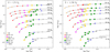 |
Fig. 4. Distribution of spectral types across the HR diagram at SMC (left panel) and one-thirtieth solar (right panel) metallicity. |
In Fig. 4 the upper left part of the HR diagram is populated by stars earlier than O5. The number of such stars is higher than at solar metallicity (see Fig. 7 of Martins & Palacios 2017). The reason for this is mainly the shift of the ZAMS and evolutionary tracks towards higher Teff at lower metallicity (Maeder & Meynet 2001). Higher Teff, and therefore earlier spectral types, are therefore reached at lower metallicity.
In Fig. 5 we show the distribution of luminosity classes in the HR diagram. This distribution at the metallicity of the SMC is different from that obtained at solar metallicity (Martins & Palacios 2017). One of the key predictions of the solar case is that (super)giants may be found early on the MS. For instance, the 100 M⊙ track at solar metallicity is populated only by supergiants (see Martins & Palacios 2017). For the SMC, giants and supergiants appear later in the evolution. This is simply understood as an effect of metallicity on stellar winds. As discussed by Martins & Palacios (2017), most luminosity class diagnostics are sensitive to wind density. As mass-loss rates and terminal velocities are metallicity dependent (Leitherer et al. 1992; Vink et al. 2001; Mokiem et al. 2007a), being weaker at lower Z, a supergiant classification is reached only for later evolutionary phases, where winds are stronger. In other words, two stars with the same effective temperature and luminosity but different metallicities will have the same position in the HR diagram but will have different luminosity classes. For similar reasons, Martins & Palacios (2017) showed that O2V stars were not encountered at solar metallicity, as confirmed by observations. For a star to have an O2 spectral type it needs to have a high effective temperature, above 45 000 K. This is feasible for massive and luminous stars only. In the Galaxy, at high luminosities the winds are strong enough to impact the main luminosity class diagnostic line (He II 4686). Consequently, all O2 stars are either giants or supergiants. At the reduced metallicity of the SMC, He II 4686 is less filled with wind emission and a dwarf classification is possible. From Table A.1, we see that O2V objects are found in the early MS of the 150 M⊙ track, and possibly also of the 80 and 100 M⊙ tracks (here the ZAMS models are classified O2−3V). The O2V classification is confined to the most massive stars but is not unexpected.
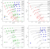 |
Fig. 5. Hertzsprung-Russell diagrams at Z = 1/5 Z⊙ with the various luminosity classes indicated by symbols and colors. Top left panel: all luminosity classes, top right (respectively bottom left and bottom right) panel: focuses on dwarfs (respectively on giants and supergiants). Small open symbols are SMC stars analyzed by Mokiem et al. (2006), Bouret et al. (2013), Castro et al. (2018), Ramachandran et al. (2019) and Bouret et al. (in prep.). |
In Fig. 5 we also compare our predictions to the position of observed SMC stars. According to our predictions, dwarfs cover most of the MS range for masses up to 40 M⊙. Above that mass, giants appear soon after the ZAMS and are found over a large fraction of the MS. The observed distribution of dwarfs is relatively well accounted for by our models (see top right panel of Fig. 5). We note that there is a significant overlap between observed dwarfs and giants making a more quantitative comparison difficult. For instance, both luminosity classes are encountered near the terminal-age main sequence (TAMS) of the 20 M⊙ track. The three 20 M⊙ models immediately before, at, and immediately after the TAMS have luminosity classes IV, III−I, and IV, respectively (see Table A.1). This is globally consistent with observations.
We predict supergiants only at or after the TAMS, except for the 150 M⊙ track where they appear in the second part of the MS. Observations indicate that supergiants populate a hotter region of the HRD on average. This mismatch may be due to incorrect mass-loss rates in our computations that would produce weaker wind-sensitive lines (see below). If real, this phenomenon should also affect the position of giants (our predictions should be located to the right of the observed giants). Given the overlap between dwarfs and giants described above, we are not able to see if the effect is present. In our models, we introduce a mass-loss reduction by a factor of three due to clumping, which is a standard value for Galactic stars (Cohen et al. 2014). At the metallicity of the SMC, one may wonder whether this factor is the same. If it was smaller, wind-sensitive lines, which mostly scale with  where f is the clumping factor6 would be slightly stronger than in our models. Marchenko et al. (2007) concluded that there is no metallicity dependence of the clumping properties but their conclusion is based on a small sample of Wolf-Rayet stars. In addition these objects have winds that do not behave exactly as those of OB stars (e.g., Sander et al. 2017). Finally, rotation, which is not included in our evolutionary models, could slightly strengthen winds and affect luminosity class determination. However, supergiants usually rotate slowly and this effect should be negligible.
As highlighted by Ramachandran et al. (2019), whose data are included in Fig. 5, there seems to be a quasi absence of observed stars above 40 M⊙. Castro et al. (2018) indicated that SMC stars were not observed above ∼40 M⊙ in the classical Hertzsprung-Russel diagram, but were found in the spectroscopic HR diagram (Langer & Kudritzki 2014), a modified diagram where the luminosity L is replaced by  where g is the surface gravity. Castro et al. (2018) attributed this difference to the so-called mass discrepancy problem, namely that masses determined from the HR diagram are different from those obtained from surface gravity (Herrero et al. 1992; Markova et al. 2018). Dufton et al. (2019) focused on NGC 346 in the SMC and again found no stars more massive than 40 M⊙ in their HRD. The absence of the most massive OB stars in the SMC therefore seems to be confirmed by several independent studies relying on different atmosphere and evolutionary models. Since the distance to the SMC is well constrained, luminosities should be safely determined as well. Ramachandran et al. (2019) concluded that stellar evolution above 40 M⊙ in the SMC must be different from what is predicted at higher metallicity. These latter authors argued that quasi-chemically homogeneous evolution may be at work. This peculiar evolution is expected for fast-rotating stars (Maeder 1987; Yoon et al. 2006): due to strong mixing, the opacity is reduced and the effective temperature increases along the evolution, instead of decreasing for normal MS stars. Consequently, stars evolve to the left part of the HRD, directly after the ZAMS. There is indeed evidence that at least some stars in the SMC follow this path (Martins et al. 2009). These objects are classified as early WNh stars; their effective temperatures are high and their chemical composition is closer to that of OB stars than to that of evolved Wolf-Rayet stars. These properties are consistent with quasi-chemically homogeneous evolution. Bouret et al. (2003, 2013) also suggested such evolution for the giant MPG 355. This giant is reported in the bottom left panel of Fig. 5 as the open green square just right of the ZAMS at
  ∼ 6.0. Its high nitrogen content and its peculiar position may be consistent with quasi-homogeneous evolution, although the measured V sin i remains modest (120 km s−1, see also Rivero González et al. 2012). Whether or not stellar evolution above ∼40 M⊙ follows a peculiar path in the SMC is not established, but our study indicates that this possibility should be further investigated. A final, alternative possibility to explain the lack of stars more massive than about 60 M⊙ at SMC metallicity is a different star formation process or at least different star formation conditions compared to solar metallicity environments.
We conclude this section by commenting in general on the behavior of optical and UV spectra. In Fig. 6 we illustrate that stars displaying similar helium lines in the optical, and therefore of similar spectral type, can have different UV spectra. Here, we focus on the models of the Z = 1/5 Z⊙ grid that have been classified as O4V((f)) or O5V((f)). These correspond to stars with initial masses ranging from 40 to 60 M⊙. We see that despite having similar spectral types, the strength of the wind features increases with initial mass. More massive stars are also more luminous and, as mass-loss rates are sensitive to luminosity (e.g., Björklund et al. 2021), this translates into stronger P Cygni features. However the winds are not strong enough to cause He II 4686 to enter the regime of giants or supergiants and the models remain classified as dwarfs. For a given mass, the luminosity effect is also observed as the star evolves off the ZAMS: the C IV 1550 line is stronger in the 40 M⊙ model classified as O5V((f)), which is also more evolved and more luminous than the 40 M⊙ model classified as O4V((f)) (see Table A.1).
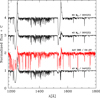 |
Fig. 6. Ultra-violet spectra of the models of the Z = 1/5 Z⊙ series for which a spectral type O4V((f)) or O5V((f)) was attributed (see Table A.1). The HST/COS spectrum of the O4−5V star AzV 388 in the SMC, from Bouret et al. (2013), is inserted in red. The main lines are indicated. The initial masses of the models are also given. |
For comparison, and as a sanity check, we added the spectrum of the SMC star AzV 388 (O4−5V) in Fig. 6. The goal is not to provide a fit of the observed spectrum but to assess whether or not our models are broadly consistent with typical features observed in the SMC. The two strongest lines of AzV 388 (N V 1240 and C IV 1550) have intensities comparable to our 40 M⊙ model classified O5V((f)). Bouret et al. (2013) determined Teff = 43 100 K and  = 5.54 for AzV 388. These properties are very similar to those of our O5V((f)) model (Teff = 43 614 K and
  = 5.50, see Table A.1). The morphology of UV spectra we predict is therefore broadly consistent with what is observed in the SMC. The larger v∞ in our model (3496 km s−1 versus 2100 km s−1 for AzV 388 according to Bouret et al. 2013) explains the larger blueward extension of the P Cygni profiles in our model.
3.3. One-thirtieth solar metallicity
We now turn to the Z = 1/30 Z⊙ grid. Before discussing the predicted spectroscopic sequences, we first look at how our evolutionary tracks compare with other computations in this recently explored metallicity regime.
3.3.1. Comparison of evolutionary models
In this section we consider the tracks of Szécsi et al. (2015) and Groh et al. (2019) which assume Z = 1/50 Z⊙ and Z = 1/35 Z⊙ respectively. The comparisons for tracks with similar masses are shown in Fig. 7. In general, we find good agreement between all predictions. The Groh et al. and Szésci et al. tracks start at slightly higher Teff than our models. This is easily explained by the metallicity differences, with stars with less metals having higher Teff. The tracks by Groh et al. (2019) are on average 0.02−0.03 dex more luminous. Additionally, they have very similar shapes to our tracks, especially near the TAMS. The tracks by Szécsi et al. (2015) are 0.03 to 0.12 dex more luminous than ours. The difference is larger (smaller) for lower (higher) initial masses and is mainly attributed to the smaller metallicity. Due to the very large core overshooting they adopt in their models (more than three times as large as the one adopted in this work and in Groh et al. 2019) as commented in their paper, the non-rotating models by Szécsi et al. (2015) reach the TAMS at much lower effective temperature than our models. This can be seen on their low mass tracks, which are interrupted before they reach the short contracting phase translated into a hook at the TAMS of classical models. For the 100 M⊙ and 150 M⊙ models, the Szecsi et al. models become underluminous compared to ours near logTeff = 4.55, because they are still undergoing core H burning while our models have switched to core He burning and have undergone thermal readjustment at the end of core H burning.
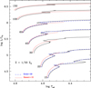 |
Fig. 7. Comparison of evolutionary models without rotation at Z = 1/30 Z⊙ (our calculations in black solid lines), Z = 1/35 Z⊙ from Groh et al. (2019) (blue dashed lines), and Z = 1/50 Z⊙ from Szécsi et al. (2015) (red dotted lines). Initial masses are indicated at the beginning of each evolutionary sequence. For the Szécsi et al. (2015) 40 and 60 M⊙ tracks the actual values of the initial masses are respectively 39 and 59 M⊙. |
Let us finally note the hooks in our 15 and 20 M⊙ tracks below logTeff ≈ 4.4. These correspond to the onset of core helium burning and are a known feature of models with very moderate overshooting and a core convection defined by the Schwarzschild criterion (Sakashita et al. 1959; Iben 1966; Kippenhahn et al. 2012).
3.3.2. Spectroscopic sequences at Z = 1/30 Z⊙
The right panel of Fig. 4 as well as Table A.2 reveal that, above 40 M⊙, stars at Z = 1/30 Z⊙ spend almost the entire MS as O2 to O6 stars, with a significant fraction of the MS spent in the earliest spectral types (i.e., < O4.5). We predict that 100 and 150 M⊙ stars spend a non-negligible part of their evolution as O2 stars. We therefore expect a large fraction of early-type O stars in young massive clusters in this metallicity range. For comparison, NGC 3603, one of the youngest and most massive cluster in the Galaxy, has fifteen O3−O4 stars but no O2 star (Melena et al. 2008). The reason for this is the higher effective temperature of lower metallicity stars (e.g., Mokiem et al. 2007b), and their corresponding earlier spectral types. In our spectroscopic sequences at Z = 1/30 Z⊙ most of the O2 stars are dwarfs.
Kubátová et al. (2019) calculated theoretical spectra of metal-poor stars (Z = 1/50 Z⊙) following quasi chemically homogeneous evolution. This type of evolution is different from the one followed in our computations, because it requires that rotational mixing be taken into account. However, the ZAMS models of Kubátová et al. (2019) can be compared to our results. Kubátová et al. assign a spectral type O8.5−O9.5V to their ZAMS 20 M⊙ model, for which Teff = 38 018 K,  = 4.68, and log g = 4.35. These parameters are close to our 20 M⊙ ZAMS model (see Table A.2) which we classify as O7.5V((f)). The slightly larger Teff and log g in our model easily explain the small difference in spectral type. The 60 M⊙ ZAMS model of Kubátová et al. (2019) has Teff = 54 954 K,
  = 5.75, and log g = 4.39, again very similar to our corresponding 60 M⊙ model. We assign a O3−3.5V((f)) classification to our model, while Kubátová et al. (2019) prefer < O4III. We therefore agree on the spectral type but find a different luminosity class. The latter is based in the strength of He II 4686. As we use a mass-loss rate that is about 0.5 dex smaller than that used by Kubátová et al., we naturally predict a weaker He II 4686 emission, which explains the different luminosity classes. The global spectral classification between both sets of models is therefore relatively consistent, considering that different metallicities are used (1/30 Z⊙ for us, 1/50 Z⊙ for Kubátová et al. 2019).
The distribution of luminosity classes in our predicted spectra is shown in Fig. 8. Compared to the Galactic case (see Martins & Palacios 2017), the match between MS and luminosity class V is almost perfect up to M ∼ 60 M⊙. Giants populate an increasingly large fraction of the MS at higher masses. At a metallicity of 1/30 Z⊙, and below 60 M⊙, a dwarf luminosity class is therefore quasi-equivalent to a MS evolutionary status. For M = 15 M⊙ we do not predict supergiants even in the early phases of the post-MS evolution that we cover (they may appear later on, at lower Teff). In our computations, supergiants are seen only in the post-MS phase of stars more massive than 20 M⊙.
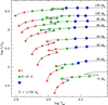 |
Fig. 8. Hertzsprung-Russell diagram at Z = 1/30 Z⊙ with the various luminosity classes indicated by symbols and colors. |
There is so far only one O star detected in a Z = 1/30 Z⊙ galaxy (Leo P, Evans et al. 2019). There are a few hot massive stars detected in Local Group galaxies with metallicities between that of the SMC and 1/10 Z⊙ (Bresolin et al. 2007; Evans et al. 2007; Garcia & Herrero 2013; Hosek et al. 2014; Tramper et al. 2014; Camacho et al. 2016; Garcia 2018; Garcia et al. 2019). An emblematic galaxy in the low-metallicity range is I Zw 18 (Z ∼ 1/30−1/50 Z⊙, Izotov et al. 1999) in which Izotov et al. (1997) reported the detection of Wolf-Rayet stars (see also Brown et al. 2002). No OB star has yet been observed in I Zw 18 in spite of strong nebular He II 4686 emission (Kehrig et al. 2015) which is difficult to reproduce with standard stellar sources (e.g., Schaerer et al. 2019). Comparison of the distribution of spectral types and luminosity classes at Z = 1/30 Z⊙ is therefore not feasible at present. Garcia et al. (2017) showed in their Fig. 2 a HR diagram for stars in Local Group galaxies with Z ∼ 1/5−1/10 Z⊙. The most massive objects are O stars with masses ∼60 M⊙. The absence of more massive stars that, according to our predictions, should appear as early-O type stars, may be an observational bias. Alternatively, this absence may also extend the results obtained in the SMC: the most massive OB stars may be absent in these low-metallicity environments, for a reason that remains unknown.
The right panels of Figs. 2 and 3 show the spectroscopic sequences of the 60 M⊙ models at Z = 1/30 Z⊙ (see Figs. B.1 and B.2 for the 20 M⊙ models). As previously noted, the line strengths in the UV range are strongly reduced compared to the SMC case. Most lines usually showing a P Cygni profile in OB stars are almost entirely in absorption. For M = 60 M⊙ only N V 1240 and C IV 1550 show a P Cygni profile in early/mid O dwarfs and late-O/early-B supergiants, respectively. A similar behavior is observed for the most massive star we study (M = 150 M⊙, see Fig. B.4). For M = 20 M⊙, C IV 1550 is the only line developing into a weak P Cygni profile. According to the scaling of mass-loss rates with metallicity (Ṁ ∝ Z0.7−0.8, see Vink et al. 2001; Mokiem et al. 2007a), these rates should be approximately three to four times lower at Z = 1/30 Z⊙ than at SMC metallicity (1/5 Z⊙) and about 15 times lower than in the Galaxy. Bouret et al. (2015) and Garcia et al. (2017) show HST UV spectra of O stars in IC 1613, WLM, and Sextans A, three Local Group galaxies with metallicities between 1/5 and 1/10 Z⊙. In IC 1613 and WLM (Z = 1/5 Z⊙), the P Cygni profiles are weak but still observable; their strength is comparable to that of SMC stars (see Fig. 4 of Garcia et al. 2017). In the spectrum of the Sextans A O7.5III((f)) star presented by Garcia et al. (2017), most wind-sensitive lines are in absorption. Other O stars in Sextans A show the same behavior (M. Garcia, priv. comm.). In view of the lower metallicity of Sextans A (Z = 1/10 Z⊙), this is consistent with the expectation of the reduction of mass-loss rates at lower metallicity.
3.4. Optical wavelength range of the ELT
Local Group dwarf galaxies are prime targets to hunt for OB stars beyond the Magellanic Clouds (Camacho et al. 2016; Garcia & Herrero 2013; Evans et al. 2019); most of them have low metallicity (McConnachie et al. 2005). Current facilities barely collect low-spectral-resolution and low-signal-to-noise-ratio data for a few of their OB stars. The advent of the new generation of ground-based ELTs assisted with sophisticated adaptive-optics systems will likely lead to a breakthrough in the detection of low-metallicity massive stars. In particular, two instruments planned for the European ELT will have integral-field units or multi-objects spectroscopic capabilities: HARMONI and MOSAIC7. These instruments will have resolving power of at least a few thousand and will have a wavelength coverage from ∼4500 Å to the K-band. They will therefore not entirely cover the classical optical range from which most of the spectroscopic diagnostic lines have been defined (Conti & Alschuler 1971; Walborn 1972; Mathys 1988; Sota et al. 2014; Martins 2018).
In Figs. 9 and 10 we show our predicted spectra for 60 M⊙ stars at SMC and one-thirtieth solar metallicities. We focus on the wavelength range 4500−8000 Å which will be probed by HARMONI and MOSAIC. We selected this range for the following reasons: it contains a fair number of lines from different elements; at these wavelengths, OB stars emit more flux than in the near-infrared; Local Group dwarf galaxies have relatively low extinction (Tramper et al. 2014; Garcia et al. 2019). We therefore anticipate that it will be more efficient to detect and characterize new OB stars in this wavelength range.
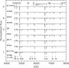 |
Fig. 9. Spectra of the sequence of models calculated along the 60 M⊙ track at SMC metallicity in the blue spectral range of ELT/HARMONI and ELT/MOSAIC. The main diagnostic lines are indicated. The spectra have been degraded to a spectral resolution of approximately 5000, which is typical of the ELT instruments. A rotational velocity of 100 km s−1 has been considered for all spectra. |
Figures 9 and 10 show that several He I and He II lines are present in the selected wavelength range. In particular, many He II lines from the n = 5 (ground-state principal quantum number equal to 5) series are visible. The change in ionization when moving from the hottest O stars to B stars is clearly seen. For instance, the He II lines at 5412 Å and 7595 Å weaken when the He I lines at 5876 Å and 7065 Å strengthen. Effective temperature determinations based on spectral features observed with ELT instruments should therefore be relatively straightforward provided nebular lines do not produce too much contamination. Hβ, a classical indicator of surface gravity (Martins 2011; Simón-Díaz 2020), is also available. At slightly longer wavelengths, between 8000 and 9000 Å (a range that will be covered by HARMONI and MOSAIC but not shown here), the Paschen series offers numerous hydrogen lines that are also sensitive to log g (Negueruela et al. 2010). Surface gravity will therefore be easily determined from ELT observations.
The wavelength considered in Figs. 9 and 10 contains a few lines from carbon, nitrogen, and oxygen, but less than the bluer part (3800−4500 Å). The strongest lines are C IV 5805−5812, N III 4640, and O III 5592. At longer wavelengths, there are even fewer CNO lines (see Fig. B.3 for the K-band). The determination of CNO abundances of OB stars will therefore be more difficult than in the more classical optical and UV spectra where tens of lines are available (e.g., Martins et al. 2015). Si IV 7718, which is found next to C IV 7726, is a relatively strong line in the earliest O stars that may turn useful for metallicity estimates.
Hα will be observed by ELT instruments. It is a classical mass-loss-rate indicator because the photospheric component is filled with wind emission (Repolust et al. 2004). However, below about 10−7 M⊙ yr−1 the wind contribution vanishes. Other hydrogen lines from the Paschen and Brackett series are present in the JHK bands, but they are weaker than Hα. Since mass-loss rate scales with metallicity (Vink et al. 2001; Mokiem et al. 2007a) we anticipate that only upper limits on this parameter will be obtained for all but the most luminous and evolved OB stars in low-metallicity environments, unless complementary UV data are acquired.
Based on the evolution of spectral lines seen in Figs. 9 and 10 we have identified a potential criterion for spectral classification in the wavelength range 4500−8000 Å that will be covered by both HARMONI and MOSAIC. Helium lines are the prime diagnostics of spectral types among O stars (Conti & Alschuler 1971; Mathys 1988). We measured the EW of various He I and He II lines, computed their ratios, and plotted them against the estimated spectral types. We did this for the two sets of models (SMC and one-thirtieth solar metallicity). More specifically, we considered He I 4713, He I 4920, He I 5876, He I 7065, He II 4542, and He II 5412. We find that the ratio EW(He I 7065)/EW(He II 5412) shows a monotonic and relatively steep evolution through spectral types. In addition, the two lines are not particularly close to the blue part of the spectral range considered, where detectors may be less efficient. We show the trends we obtained in Fig. 11. There is no difference among the two metallicities: at a given spectral type, the EW ratios of the two metallicities overlap (see right panel of Fig. 11). To further investigate the potential of this indicator, we added our solar metallicity models (from Martins & Palacios 2017). Again, the EW ratios are similar to the lower metallicity models. A final check was made by incorporating measurements from Galactic stars: these are the red points in Fig. 11. We relied on archival data from CFHT/ESPaDOnS, TBL/NARVAL, and ESO/FEROS. The details of the data are given in Appendix C. The reduced observed spectra were normalized and EWs were measured in the same way as for the model spectra. We see that from spectral types O5.5 to B0.5 the agreement between the observed EW ratios and the model ratios is excellent. We note a small offset at earlier spectral types (O3 to O5). This may be caused by several factors: (1) the small number of observed spectra in that spectral type range; (2) the use of additional criteria – namely nitrogen lines – to refine spectral classification, particularly at O3, O3.5 and O4; and (3) the increasing weakness of He I 7065 in that range and consequently the stronger impact of neighboring Si IV and C IV lines, the modeling of which needs to be tested. We also stress that at spectral type O5 a similar offset was observed in the classical EW(He I 4471)/EW(He II 4542) ratio shown in Fig. 1 of Martins (2018). In view of these results, we advocate the ratio EW(He I 7065)/EW(He II 5412) as a reliable spectral type criterion in the wavelength range 4500−8000 Å, especially for spectral types between O5.5 and B0.5. It can be used for classification of O and early-B stars in Local Group galaxies observed with the ELT.
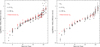 |
Fig. 11. Ratio of the EW of He I 7065 to He II 5412 as a function of spectral type for the low-metallicity models calculated in the present study, the solar metallicity models of Martins & Palacios (2017) and observations of Galactic stars collected from archives (open red circles – see text for details). Left panel: all data points shown. When no unique spectral type was assigned to a model (e.g., O6−6.5) the average was used (i.e., O6.25). Numbers above ten correspond to B stars (with ten being B0, and 10.5 being B0.5). Right panel: same as left panel but showing only the average value of the EW ratio for each spectral type. In that panel the spectral types of the 1/5 Z⊙ (1/30 Z⊙) models have been shifted by +0.03 (−0.03) for clarity. We also considered only “official” spectral types, that is, we excluded for example 6.25 when a spectral type O6−6.5 was assigned to a model. |
4. Ionizing properties and He II 1640 emission
In this section we describe the ionizing properties of our models and study their dependence on metallicity. We also describe the morphology of He II 1640 in our models, a feature that depends on the ionizing power of stars in star-forming galaxies.
4.1. Ionizing fluxes
Here we first discuss the hydrogen ionizing flux before turning to the helium ionizing fluxes. All ionizing fluxes of our models are given in Tables A.1 and A.2.
4.1.1. Hydrogen ionizing flux
In Fig. 12 we compare the ionizing fluxes per unit surface area – q(H)8 – for three metallicities: solar, one-fifth solar, and one-thirtieth solar (see top panel). At the highest Teff the relation between logq(H) and Teff is very narrow. When Teff decreases, a dispersion in logq(H) for a given Teff appears. This is explained by the effect of surface gravity on SEDs (see detailed physics in Abbott & Hummer 1985) and the wider range of surface gravities covered by cooler models. Indeed, a look at Fig. 1 and Tables A.1 and A.2 indicates that the hottest models correspond to MS stars with high surface gravities, while lower Teff models can be either MS or post-MS models, with a wide range of log g. Figure 12 does not reveal any strong metallicity dependence of the relation between hydrogen ionizing fluxes (per unit surface area) and effective temperature. At high Teff the (small) dispersion of q(H) for a given Teff is larger than any variation of q(H) with Z that may exist. At the lowest effective temperatures, the lower limit of the q(H) values is the same for all metallicities. The upper boundary of q(H) is located slightly higher at low Z. We stress that because luminosities are higher at lower Z for a given Teff (see Fig. 1), radii are also larger and consequently Q(H) are higher (for a given Teff).
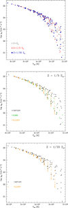 |
Fig. 12. H I ionizing fluxes per unit surface area as a function of effective temperature. Upper panel: ionizing fluxes for the two metallicities considered in this work and our solar metallicity models (Martins & Palacios 2017). Middle and bottom panel: 1/5 Z⊙ and 1/30 Z⊙ models, respectively, which are compared to TLUSTY (Lanz & Hubeny 2003) and PoWR (Hainich et al. 2019) models. |
Figure 13 illustrates how the SED changes when the metal content and mass-loss rate are modified, all other parameters being kept constant. As discussed at length by Schaerer & de Koter (1997) the variations in opacity and wind properties affect the SED. An increase of the metal content from 1/30 Z⊙ to 1/5 Z⊙ strengthens the absorption due to lines. The consequence is a reduction of the flux where the line density is the highest. This is particularly visible in Fig. 13 between 250 and 400 Å. A stronger opacity also affects the continua, especially the He II continuum below 228 Å. However, in the case illustrated in Fig. 13, we also note that the redistribution of the flux from short to long wavelengths (due to increased opacities and to ensure luminosity conservation) takes place mainly below the hydrogen ionizing edge: the flux in the lowest metallicity model is higher (smaller) than the flux in the Z = 1/5 Z⊙ model below (above) ∼550 Å. But above 912 Å, both models have the same flux level. Consequently, logq(H) is almost unchanged (24.15 vs. 24.17). Figure 13 also reveals that variations in mass-loss rate for the model investigated here have little effect on the hydrogen ionizing flux, whereas the He II ionizing flux is affected (see following section).
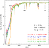 |
Fig. 13. Effect of metallicity on the SED. The initial model (red line) is the fifth model of the 60 M⊙ series at Z = 1/30 Z⊙. The blue line shows the same model for which the metallicity has been changed to 1/5 Z⊙, all other parameters being kept constant. In the model shown by the orange line, in addition to metallicity, the mass-loss rate has been increased by a factor 4.2 according to Ṁ ∝ Z0.8. Finally, in the model shown in green, the mass-loss rate has been reduced down to log Ṁ = −7.30. The H I, He I, and He II ionizing edges are indicated by vertical black lines. |
In the middle and bottom panels of Fig. 12 we compare our hydrogen ionizing fluxes to the results of Lanz & Hubeny (2003) obtained with the code TLUSTY and Hainich et al. (2019) obtained with the code PoWR (Sander et al. 2015). For the latter we used the “moderate” mass-loss grid9 and we checked that the choice of mass-loss rates does not impact the conclusions. At high Teff the values of q(H) of the three sets of models are all consistent within the dispersion. At lower Teff our predictions have the same lower envelope as Hainich et al. (2019), while the plane-parallel models of Lanz & Hubeny (2003) have slightly lower fluxes. Our ionizing fluxes reach higher values than the two other sets of models for a given Teff. These differences are readily explained by the wider range of log g covered by our models. Taking Teff ∼ 27 000 K as a representative case, the grids of Lanz & Hubeny (2003) and Hainich et al. (2019) do not include models with log g < 3.0 while we have a few models with log g ∼ 2.7. The models of Lanz & Hubeny (2003) also reach higher log g (up to 4.75) which explains the small difference in the minimum fluxes. The same conclusions are reached at Z = 1/30 Z⊙. Different sets of models therefore agree well as far as the hydrogen ionizing fluxes per unit area are concerned.
4.1.2. Helium ionizing fluxes
In this section we now focus on the ratios of helium to hydrogen ionizing fluxes because they are a common way of quantifying the hardness of a stellar spectrum. It is also a convenient way of investigating the effects of metallicity on stellar SEDs.
Figure 14 shows the ratios of He I and He II to H I ionizing fluxes as a function of Teff for the two metallicities considered in the present study. We have also added our results for the solar metallicity calculations of Martins & Palacios (2017). The  ratio displays a very well-defined sequence down to ∼35 000 K for each metallicity. At lower temperatures, the ratios drop significantly and the dispersion increases mainly because of the strong reduction of the He I ionizing flux. The general trend of the
  is similar: a shallow reduction as Teff decreases down to a temperature that depends on the metallicity (see below) followed by a sharp drop. The dispersion at high Teff is larger than that of the
  ratio.
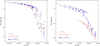 |
Fig. 14. Ratio of He I (left) or He II (right) to H I ionizing fluxes as a function of effective temperature for the two metallicities considered in this work. We have also added the models of Martins & Palacios (2017) at solar metallicity. |
This latter ratio shows a weak but clear metallicity dependence at Teff > 35 000 K in the sense that lower metallicity stars have higher ratios. The difference between solar and one-thirtieth solar metallicity reaches ∼0.2 dex at most. For Teff < 35 000 K, the larger dispersion blurs any metallicity dependence that may exist, although lower metallicity models reach on average higher ratios (the upper envelope of the distribution of Z = 1/30 Z⊙ points is located above that of Z = 1/5 Z⊙ and Z⊙ ones). The higher  ratio at lower metallicity is mainly explained by the smaller effects of line blanketing when the metal content is smaller. With reduced line opacities, and since in OB stars most lines are found in the (extreme-)UV part of the spectrum, there is less redistribution of flux from short to long wavelength (e.g., Martins et al. 2002). This effect is seen in Fig. 13 between 250 and 400 Å as explained before.
The metallicity dependence of the  ratio is of a different nature. At high effective temperatures, the three sets of models have about the same ratios for a given Teff, given the rather large dispersion. At low temperatures, more metal-poor models produce higher
  ratios. At intermediate temperature, the difference between the three metallicities considered is best explained by a displacement of the Teff at which the
  ratio drops significantly. This “threshold Teff” as we refer to it in the following is located at about 45 000 K for solar metallicity models, ∼35 000 K for Z = 1/5 Z⊙, and ∼31 000 K at Z = 1/30 Z⊙. We return to an explanation of this behavior below.
Beforehand we compare in Fig. 15 our ionizing flux ratios to the predictions of Hainich et al. (2019) for Z = 1/5 Z⊙. The computations of these latter authors assume three sets of mass-loss rates (low, moderate, and high according to their nomenclature). We show them all in Fig. 15. We also add the results of Lanz & Hubeny (2003). The general shape of the  relation is the same in the three sets of computations: the main drop happens at about the same Teff. For the highest temperatures, the ratios are the same in our study and that of Lanz & Hubeny (2003). Between ∼35 000 and 50 000 K, the models of Hainich et al. (2019) are smaller by ∼0.1 dex. For the
  ratio10, the high mass-loss-rate models of Hainich et al. (2019) experience a drop at higher Teff than all other computations (ours, and those of Hainich et al. with lower mass-loss rates).
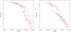 |
Fig. 15. Same as Fig. 14 but for our SMC models (red filled triangles) and comparison models of Lanz & Hubeny (2003) (open orange circles) and Hainich et al. (2019). For the latter, cyan crosses, blue squares, and purple stars correspond to low, intermediate, and high mass-loss rates, respectively. |
This behavior is similar to what we observe in the right panel of Fig. 14: different threshold Teff at different metallicities. The physical reason for this is an effect of mass-loss rates. Gabler et al. (1989, 1992) and Schaerer & de Koter (1997) studied the effects of stellar winds on the He II ionizing continuum. We refer to these works for details on the physical processes. In short, because of the velocity fields in accelerating winds, lines (in particular resonance lines) are Doppler-shifted throughout the atmosphere. They therefore absorb additional, shorter wavelength photons compared to the static case, a process known as desaturation. As a consequence, the lower level population is pumped into the higher level. The ground level opacity is reduced, leading to stronger continuum emission (Gabler et al. 1989). Schaerer & de Koter (1997) showed that this effect works as long as the recombination of doubly ionized helium into He II is moderate. On the other hand, if recombinations are sufficiently numerous, the He II ground-state population becomes overpopulated and the opacity increases, causing a strong reduction of the He II ionizing flux. Recombinations depend directly on the wind density and are therefore more numerous for high mass-loss rates.
The effects described immediately above are clearly seen in Fig. 13. Let us now focus on the models at Z = 1/5 Z⊙. Starting with the model with the smallest mass-loss rate (log Ṁ = −7.30), an increase up to log Ṁ = −6.86 translates into more flux below 228 Å. This is the regime of desaturation. A subsequent increase by another factor 4 (up to log Ṁ = −6.23) leads to a drastic reduction in the flux shortward of 228 Å. With such a high mass-loss rate, and therefore density, recombinations dominate the physics of the He II ionizing flux.
The right panel of Fig. 15 indicates that the PoWR models with the highest mass-loss rates have the smallest  ratios, at least below 45 000 K. This is fully consistent with the recombination effects. For the highest Teff the wind ionization is so high that even for strong mass-loss rates the He II ground-level population remains small. We verified that the same behavior is observed in our models. To this end, we ran new calculations for our solar metallicity grid, reducing the mass-loss rates. For selected models with Teff between 35 000 and 43 000 K, we find that the
  is increased up to the level of the low-metallicity models when mass-loss rates are reduced by a factor between 4 and 40. A stronger reduction of mass-loss rate is required for lower Teff. This is expected because at lower Teff the ionization is lower and a stronger reduction of recombinations is required to have a small ground-state opacity. As a sanity check we verified that in the initial models, with low
  ratios, He II is the dominant ion in the outer wind where the He II continuum is formed (see also Schmutz & Hamann 1986). In the models with lower mass-loss rates that have higher
  ratios, doubly ionized helium is the dominant ion in that same region, confirming the smaller recombination rates when mass-loss rates are reduced.
We conclude that our computations do show a significant metallicity dependence of the  ratio. This dependence is best described by the position of the threshold Teff at which the sudden drop between high and low
  ratios occurs. The position of this threshold temperature is physically related to mass-loss rates, as first demonstrated by Schmutz & Hamann (1986). As mass-loss rates depend on Z (Vink et al. 2001; Mokiem et al. 2007a), the
  ratio also depends on metallicity. He II ionizing fluxes are therefore sensitive to prescriptions of mass-loss rates used in evolutionary and atmosphere models.
4.2. He II 1640 emission
An interesting feature of our UV spectroscopic sequences is the presence of Lyα and He II 1640 emission in some of the models with the highest masses (see last column of Tables A.1 and A.2). Figure B.4 displays the most illustrative cases.
He II 1640 emission is a peculiar feature of some young massive clusters and star-forming galaxies both locally and at high redshift. It can be relatively narrow, and therefore considered of nebular nature, or broader and produced by stars (e.g., Cassata et al. 2013). So far, the only stars known to produce significant He II 1640 emission are Wolf-Rayet stars (Brinchmann et al. 2008; Gräfener & Vink 2015; Crowther 2019). Nebular He II emission requires ionizing photons with wavelengths shorter than 228 Å. Possible sources for such hard radiation are (in addition to Wolf-Rayet stars themselves) population III stars (Schaerer 2003), massive stars undergoing quasi-chemically homogeneous evolution (Kubátová et al. 2019), stripped binary stars (Götberg et al. 2017), X-ray binaries (Schaerer et al. 2019), and radiative shocks (Allen et al. 2008).
Saxena et al. (2020) report EW values of ∼1−4 Å in a sample of He II 1640-emitting galaxies at redshift 2.5−5.0 (see also Steidel et al. 2016; Patrício et al. 2016). Slightly larger values (5 to 30 Å) are given by Nanayakkara et al. (2019) at redshifts from 2 to 4, while values lower than 1 Å are also reported by Senchyna et al. (2017) in nearby galaxies. All these measurements include both stellar and nebular contributions. The integrated, mainly stellar He II 1640 emission of R136 in the LMC is 4.5 Å (Crowther et al. 2016; Crowther 2019). This value is similar to other (super) star clusters in the Local Universe (Chandar et al. 2004; Leitherer et al. 2018). For comparison, the EW of our models with a net emission11 reaches a maximum of ∼1.2 Å.
Gräfener & Vink (2015) studied very massive Wolf-Rayet stars with metallicities down to 0.01 Z⊙. These latter authors showed that such objects have significant He II 1640 emission that could explain observations in some super-star clusters (Cassata et al. 2013; Wofford et al. 2014). Figure 16 shows the location of our models with a net He II 1640. At the metallicity of the SMC, these are found above 80 M⊙ and in the first part of the MS. At Z = 1/30 Z⊙ stellar He II 1640 emission is produced in stars more massive than 60 M⊙ and these stars are found mainly close to the TAMS, although their location extends to earlier phases at higher masses. He II 1640 emission appears at ages between 0 and ∼2.5 Myr (Z = 1/5 Z⊙) and between ∼1.5 and ∼4 Myr (Z = 1/30 Z⊙). Compared to Gräfener & Vink (2015), we therefore predict emission in lower mass stars, which are likely more numerous in young star clusters. These may therefore contribute to the integrated light of young stellar populations. Nonetheless, we stress that our models always have He II 4686 in absorption. Consequently, if low-metallicity stars appear as we predict, they cannot account for the emission in that line observed in a number of star-forming galaxies (e.g., Kehrig et al. 2015, 2018). The different location of He II 1640 emission stars in the HRD at the two metallicities considered is explained as follows. For Z = 1/5 Z⊙ winds are stronger and therefore very hot stars are more likely to show emission. Conversely, at higher metallicity there are more metallic lines on top of the He II 1640 profile (see Fig. 17). At the temperatures typical of the TAMS, these lines are more numerous than at the ZAMS. At Z = 1/5 Z⊙ they are strong enough to produce an absorption that counter-balances the underlying He II 1640 emission. Because of the effect of these metallic lines, EWs are on average larger at lower metallicity (see Tables A.1 and A.2). Additionally, at lower Z, winds are weaker and He II 1640 does not develop an emission profile close to the ZAMS, where wind densities are too small. He II 1640 emission is therefore observed closer to the ZAMS (TAMS) at higher (lower) metallicity.
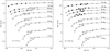 |
Fig. 16. HR diagram (Z = 1/5 Z⊙, left panel; Z = 1/30 Z⊙, right panel) showing the position of the models with He II 1640 emission (absorption) in black filled (open) squares. |
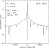 |
Fig. 17. He II 1640 profile of the model with the strongest emission. |
Figure 17 shows a zoom on the He II 1640 line of the model with the strongest emission along the 150 M⊙ sequence (Z = 1/30 Z⊙). The profile has relatively broad wings extending up to ±2000 km s−1. The central part is composed of a narrow component (∼250 km s−1 wide) with two emission peaks separated by a narrow absorption component. This narrow component is likely affected by nebular emission when present in integrated observations of stars and their surrounding nebula.
5. Conclusion
We present calculations of synthetic spectroscopy along evolutionary tracks computed at one-fifth and one-thirtieth solar metallicity. The models cover the MS and the early post-MS phases. Stellar-evolution computations were performed with the code STAREVOL, while atmosphere models and synthetic spectra were calculated with the code CMFGEN. Our models cover the mass range 15−150 M⊙. For each mass, we provide spectroscopic evolutionary sequences. This study extend our work at solar metallicity presented in Martins & Palacios (2017).
Our spectroscopic sequences all start as O dwarfs (early, intermediate, or late depending on initial mass) and end (in the early post-MS) as B giants or supergiants. The most massive stars are predicted to begin their evolution as O2V stars, contrary to solar metallicity computations for which such stars are not expected and not observed. The fraction of O2V stars increases when metallicity decreases.
At the metallicity of the SMC (Z = 1/5 Z⊙) and below 60 M⊙ stars spend a large fraction of the MS as dwarfs (luminosity class V) although the region near the TAMS is populated by giants (luminosity class IV, III, and II). Above 60 M⊙, models enter the giant phase early on the MS. Our predictions reproduce the observed distribution of dwarfs and giants in the SMC relatively well. For supergiants, the distribution we predict is located at lower Teff than observed. We confirm results presented by Castro et al. (2018) and Ramachandran et al. (2019), which show that, from the HR diagram, there seems to be a lack of stars more massive than ∼60 M⊙ in the SMC. We predict that stars with masses higher than 60 M⊙ should be observed as O and B stars with luminosities higher than 106 L⊙, but almost no such star is reported in the literature. Whether this is an observational bias or an indication of either a peculiar evolution or a quenching of the formation of the most massive stars in the SMC is not clear.
At Z = 1/30 Z⊙, a larger fraction of the MS is spent in the luminosity class V, even for the most massive models. Below 60 M⊙, the MS is populated only by luminosity class V objects. The appearance of giants and supergiants is pushed to lower Teff at low Z. This is caused by the reduced wind strength (see Martins & Palacios 2017). This reduction in the strength of wind-sensitive lines with metallicity is striking in the UV spectra. At one-thirtieth solar metallicity, only weak P Cygni profiles in N V 1240 and C IV 1550 are sometimes observed.
We also present spectroscopic sequences in the wavelength range 4500−8000 Å that will be covered by the instruments HARMONI and MOSAICS on the ELT. Hot massive stars will be best observed at these wavelengths in Local Group galaxies with low extinction. We advocate the use of the ratio of He I 7065 to He II 5412 as a new spectral class diagnostics. Using archival high-resolution spectra and our synthetic spectra, we show that this ratio is a robust criterion for spectral typing, and is independent of metallicity.
We provide the ionizing fluxes of our models. The relation between hydrogen-ionizing fluxes per unit area and Teff does not depend on metallicity. On the contrary, we show that the relations  versus Teff and
  versus Teff both depend on metallicity, although in a different way. Both relations show a shallow decrease when Teff diminishes until a sharp drop at a characteristic Teff. Below this latter point of characteristic Teff, the ratios of ionizing fluxes decrease faster. For
  , at a given Teff, low-metallicity stars have higher ratios above the drop encountered at ∼35 000 K. For
  , it is the position of the drop that is affected, being located at higher Teff for stars with higher metallicity. This behavior is rooted in the metallicity dependence of mass-loss rates.
Finally, we highlight that in some models for the most massive stars, we predict a net emission in He II 1640, a feature observed in some star-forming galaxies but difficult to reproduce in population synthesis models. The emission we predict is stronger at lower metallicity, reaching a maximum EW of the order of 1.2 Å. The line profile is composed of broad wings and a narrow core and is present in a region of the HRD near the ZAMS (TAMS) at Z = 1/5 Z⊙ (Z = 1/30 Z⊙).
Our SEDs and synthetic spectra are made available to the community through the POLLUX database.
We note that in the calculation of the mass-loss rates we use the recipe of Vink et al. (2001) which incorporates a ratio v∞/vesc of 2.6. This is slightly different from the value of 3.0 we use for the calculation of the synthetic spectra, but the difference is minimal: adopting 3.0 in the Vink formula would change the mass-loss rate by 0.08 dex, which is negligible.
A super-level approach is used in CMFGEN calculations. The ∼7100 levels are grouped in about 1800 super-levels.
We stress that theoretical predictions of mass-loss rates based on the calculation of radiative driving may not depend on the clumping factor – and therefore on its potential metallicity dependence – since clumping is usually small at the base of the atmosphere where most of the driving takes place (Sander et al. 2020).
Where  with R the stellar radius.
Data have been collected at this address http://www.astro.physik.uni-potsdam.de/PoWR/
The He II ionizing fluxes are not available for the models of Lanz & Hubeny (2003) because these are plane-parallel models and wind effects are important.
The corresponding Lyα emission is ≲2.5 Å.
Acknowledgments
We thank Andreas Sander for a prompt referee report. We warmly thank John Hillier for making the code CMFGEN available to the community and for constant help with it. We thank Daniel Schaerer for discussion on the HeII 1640 emission in star-forming galaxies. This work made use of the Polarbase database (developed and maintained by CNRS/INSU, Observatoire Midi-Pyrénées and Université Toulouse III) and of the services of the ESO Science Archive Facility.
References
- Abbott, D. C., & Hummer, D. G. 1985, ApJ, 294, 286 [NASA ADS] [CrossRef] [Google Scholar]
- Allen, M. G., Groves, B. A., Dopita, M. A., Sutherland, R. S., & Kewley, L. J. 2008, ApJS, 178, 20 [Google Scholar]
- Amard, L., Palacios, A., Charbonnel, C., Gallet, F., & Bouvier, J. 2016, A&A, 587, A105 [NASA ADS] [CrossRef] [EDP Sciences] [Google Scholar]
- Angulo, C., Arnould, M., Rayet, M., et al. 1999, Nucl. Phys. A, 656, 3 [NASA ADS] [CrossRef] [Google Scholar]
- Asplund, M., Grevesse, N., Sauval, A. J., & Scott, P. 2009, ARA&A, 47, 481 [NASA ADS] [CrossRef] [Google Scholar]
- Björklund, R., Sundqvist, J. O., Puls, J., & Najarro, F. 2021, A&A, in press, https://www.aanda.org/10.1051/0004-6361/202038384 (Paper II) [Google Scholar]
- Bouret, J. C., Lanz, T., Hillier, D. J., et al. 2003, ApJ, 595, 1182 [NASA ADS] [CrossRef] [Google Scholar]
- Bouret, J. C., Lanz, T., Martins, F., et al. 2013, A&A, 555, A1 [NASA ADS] [CrossRef] [EDP Sciences] [Google Scholar]
- Bouret, J. C., Lanz, T., Hillier, D. J., et al. 2015, MNRAS, 449, 1545 [NASA ADS] [CrossRef] [Google Scholar]
- Bresolin, F., Urbaneja, M. A., Gieren, W., Pietrzyński, G., & Kudritzki, R.-P. 2007, ApJ, 671, 2028 [NASA ADS] [CrossRef] [Google Scholar]
- Brinchmann, J., Kunth, D., & Durret, F. 2008, A&A, 485, 657 [NASA ADS] [CrossRef] [EDP Sciences] [Google Scholar]
- Brott, I., de Mink, S. E., Cantiello, M., et al. 2011, A&A, 530, A115 [NASA ADS] [CrossRef] [EDP Sciences] [Google Scholar]
- Brown, T. M., Heap, S. R., Hubeny, I., Lanz, T., & Lindler, D. 2002, ApJ, 579, L75 [NASA ADS] [CrossRef] [Google Scholar]
- Camacho, I., Garcia, M., Herrero, A., & Simón-Díaz, S. 2016, A&A, 585, A82 [NASA ADS] [CrossRef] [EDP Sciences] [Google Scholar]
- Cassata, P., Le Fèvre, O., Charlot, S., et al. 2013, A&A, 556, A68 [NASA ADS] [CrossRef] [EDP Sciences] [Google Scholar]
- Castro, N., Oey, M. S., Fossati, L., & Langer, N. 2018, ApJ, 868, 57 [NASA ADS] [CrossRef] [Google Scholar]
- Chandar, R., Leitherer, C., & Tremonti, C. A. 2004, ApJ, 604, 153 [NASA ADS] [CrossRef] [Google Scholar]
- Chiosi, C., & Maeder, A. 1986, ARA&A, 24, 329 [NASA ADS] [CrossRef] [Google Scholar]
- Coc, A., Vangioni-Flam, E., Descouvemont, P., Adahchour, A., & Angulo, C. 2004, ApJ, 600, 544 [NASA ADS] [CrossRef] [Google Scholar]
- Cohen, D. H., Wollman, E. E., Leutenegger, M. A., et al. 2014, MNRAS, 439, 908 [NASA ADS] [CrossRef] [Google Scholar]
- Conti, P. S., & Alschuler, W. R. 1971, ApJ, 170, 325 [NASA ADS] [CrossRef] [Google Scholar]
- Crowther, P. A. 2019, Galaxies, 7, 88 [CrossRef] [Google Scholar]
- Crowther, P. A., Caballero-Nieves, S. M., Bostroem, K. A., et al. 2016, MNRAS, 458, 624 [NASA ADS] [CrossRef] [Google Scholar]
- de Mink, S. E., Langer, N., Izzard, R. G., Sana, H., & de Koter, A. 2013, ApJ, 764, 166 [NASA ADS] [CrossRef] [Google Scholar]
- Decressin, T., Mathis, S., Palacios, A., et al. 2009, A&A, 495, 271 [NASA ADS] [CrossRef] [EDP Sciences] [Google Scholar]
- Donati, J. F., Semel, M., Carter, B. D., Rees, D. E., & Collier Cameron, A. 1997, MNRAS, 291, 658 [NASA ADS] [CrossRef] [MathSciNet] [Google Scholar]
- Dorn-Wallenstein, T. Z., & Levesque, E. M. 2018, ApJ, 867, 125 [NASA ADS] [CrossRef] [Google Scholar]
- Dufton, P. L., Evans, C. J., Hunter, I., Lennon, D. J., & Schneider, F. R. N. 2019, A&A, 626, A50 [CrossRef] [EDP Sciences] [Google Scholar]
- Evans, C. J., Bresolin, F., Urbaneja, M. A., et al. 2007, ApJ, 659, 1198 [NASA ADS] [CrossRef] [Google Scholar]
- Evans, C. J., Castro, N., Gonzalez, O. A., et al. 2019, A&A, 622, A129 [CrossRef] [EDP Sciences] [Google Scholar]
- Fullerton, A. W. 2011, in Active OB Stars: Structure, Evolution, Mass Loss, and Critical Limits, eds. C. Neiner, G. Wade, G. Meynet, & G. Peters, IAU Symp., 272, 136 [Google Scholar]
- Gabler, R., Gabler, A., Kudritzki, R. P., Puls, J., & Pauldrach, A. 1989, A&A, 226, 162 [NASA ADS] [Google Scholar]
- Gabler, R., Gabler, A., Kudritzki, R. P., & Mendez, R. H. 1992, A&A, 265, 656 [Google Scholar]
- Garcia, M. 2018, MNRAS, 474, L66 [NASA ADS] [CrossRef] [Google Scholar]
- Garcia, M., & Herrero, A. 2013, A&A, 551, A74 [NASA ADS] [CrossRef] [EDP Sciences] [Google Scholar]
- Garcia, M., Herrero, A., Najarro, F., Lennon, D. J., & Alejandro Urbaneja, M. 2014, ApJ, 788, 64 [NASA ADS] [CrossRef] [Google Scholar]
- Garcia, M., Herrero, A., Najarro, F., et al. 2017, in The Lives and Death-Throes of Massive Stars, eds. J. J. Eldridge, J. C. Bray, L. A. S. McClelland, & L. Xiao, IAU Symp., 329, 313 [Google Scholar]
- Garcia, M., Herrero, A., Najarro, F., Camacho, I., & Lorenzo, M. 2019, MNRAS, 484, 422 [Google Scholar]
- Götberg, Y., de Mink, S. E., & Groh, J. H. 2017, A&A, 608, A11 [NASA ADS] [CrossRef] [EDP Sciences] [Google Scholar]
- Götberg, Y., de Mink, S. E., Groh, J. H., et al. 2018, A&A, 615, A78 [NASA ADS] [CrossRef] [EDP Sciences] [Google Scholar]
- Gräfener, G., & Vink, J. S. 2015, A&A, 578, L2 [NASA ADS] [CrossRef] [EDP Sciences] [Google Scholar]
- Groh, J. H., Meynet, G., & Ekström, S. 2013, A&A, 550, L7 [NASA ADS] [CrossRef] [EDP Sciences] [Google Scholar]
- Groh, J. H., Meynet, G., Ekström, S., & Georgy, C. 2014, A&A, 564, A30 [NASA ADS] [CrossRef] [EDP Sciences] [Google Scholar]
- Groh, J. H., Ekström, S., Georgy, C., et al. 2019, A&A, 627, A24 [NASA ADS] [CrossRef] [EDP Sciences] [Google Scholar]
- Grunhut, J. H., Wade, G. A., Neiner, C., et al. 2017, MNRAS, 465, 2432 [NASA ADS] [CrossRef] [Google Scholar]
- Hainich, R., Ramachandran, V., Shenar, T., et al. 2019, A&A, 621, A85 [NASA ADS] [CrossRef] [EDP Sciences] [Google Scholar]
- Herrero, A., Kudritzki, R. P., Vilchez, J. M., et al. 1992, A&A, 261, 209 [NASA ADS] [Google Scholar]
- Hillier, D. J., & Miller, D. L. 1998, ApJ, 496, 407 [NASA ADS] [CrossRef] [Google Scholar]
- Hosek, M. W., Jr., Kudritzki, R. P., Bresolin, F., et al. 2014, ApJ, 785, 151 [NASA ADS] [CrossRef] [Google Scholar]
- Iben, I., Jr. 1966, ApJ, 143, 516 [NASA ADS] [CrossRef] [Google Scholar]
- Iliadis, C., D’Auria, J. M., Starrfield, S., Thompson, W. J., & Wiescher, M. 2001, ApJS, 134, 151 [NASA ADS] [CrossRef] [Google Scholar]
- Izotov, Y. I., Foltz, C. B., Green, R. F., Guseva, N. G., & Thuan, T. X. 1997, ApJ, 487, L37 [NASA ADS] [CrossRef] [Google Scholar]
- Izotov, Y. I., Chaffee, F. H., Foltz, C. B., et al. 1999, ApJ, 527, 757 [NASA ADS] [CrossRef] [Google Scholar]
- Japelj, J., Vergani, S. D., Salvaterra, R., et al. 2018, A&A, 617, A105 [NASA ADS] [CrossRef] [EDP Sciences] [Google Scholar]
- Kehrig, C., Vílchez, J. M., Pérez-Montero, E., et al. 2015, ApJ, 801, L28 [NASA ADS] [CrossRef] [Google Scholar]
- Kehrig, C., Vílchez, J. M., Guerrero, M. A., et al. 2018, MNRAS, 480, 1081 [NASA ADS] [Google Scholar]
- Keszthelyi, Z., Meynet, G., Georgy, C., et al. 2019, MNRAS, 485, 5843 [NASA ADS] [CrossRef] [Google Scholar]
- Kippenhahn, R., Weigert, A., & Weiss, A. 2012, Stellar Structure and Evolution (Berlin, Heidelberg: Springer-Verlag) [Google Scholar]
- Kobulnicky, H. A., Kiminki, D. C., Lundquist, M. J., et al. 2014, ApJS, 213, 34 [NASA ADS] [CrossRef] [Google Scholar]
- Krtička, J., & Kubát, J. 2017, A&A, 606, A31 [NASA ADS] [CrossRef] [EDP Sciences] [Google Scholar]
- Kubátová, B., Szécsi, D., Sander, A. A. C., et al. 2019, A&A, 623, A8 [NASA ADS] [CrossRef] [EDP Sciences] [Google Scholar]
- Langer, N., & Kudritzki, R. P. 2014, A&A, 564, A52 [NASA ADS] [CrossRef] [EDP Sciences] [Google Scholar]
- Lanz, T., & Hubeny, I. 2003, ApJS, 146, 417 [NASA ADS] [CrossRef] [Google Scholar]
- Leitherer, C., Robert, C., & Drissen, L. 1992, ApJ, 401, 596 [NASA ADS] [CrossRef] [Google Scholar]
- Leitherer, C., Byler, N., Lee, J. C., & Levesque, E. M. 2018, ApJ, 865, 55 [NASA ADS] [CrossRef] [Google Scholar]
- Longland, R., Iliadis, C., Champagne, A. E., et al. 2010, Nucl. Phys. A, 841, 1 [NASA ADS] [CrossRef] [Google Scholar]
- Lucy, L. B. 2010, A&A, 524, A41 [NASA ADS] [CrossRef] [EDP Sciences] [Google Scholar]
- Maeder, A. 1987, A&A, 178, 159 [NASA ADS] [Google Scholar]
- Maeder, A., & Meynet, G. 2000, ARA&A, 38, 143 [Google Scholar]
- Maeder, A., & Meynet, G. 2001, A&A, 373, 555 [NASA ADS] [CrossRef] [EDP Sciences] [Google Scholar]
- Mahy, L., Sana, H., Abdul-Masih, M., et al. 2020, A&A, 634, A118 [NASA ADS] [CrossRef] [EDP Sciences] [Google Scholar]
- Maíz Apellániz, J., Sota, A., Walborn, N. R., et al. 2011, in Highlights of Spanish Astrophysics VI, eds. M. R. Zapatero Osorio, J. Gorgas, J. Maíz Apellániz, J.~R. Pardo, & A. Gil de Paz, 467 [Google Scholar]
- Maíz Apellániz, J., Sota, A., Morrell, N. I., et al. 2013, Massive Stars: From alpha to Omega, 198 [Google Scholar]
- Marchenko, S. V., Foellmi, C., Moffat, A. F. J., et al. 2007, ApJ, 656, L77 [NASA ADS] [CrossRef] [Google Scholar]
- Markova, N., Puls, J., & Langer, N. 2018, A&A, 613, A12 [NASA ADS] [CrossRef] [EDP Sciences] [Google Scholar]
- Martins, F. 2011, Bull. Soc. R. Sci. Liege, 80, 29 [Google Scholar]
- Martins, F. 2018, A&A, 616, A135 [NASA ADS] [CrossRef] [EDP Sciences] [Google Scholar]
- Martins, F., & Palacios, A. 2013, A&A, 560, A16 [NASA ADS] [CrossRef] [EDP Sciences] [Google Scholar]
- Martins, F., & Palacios, A. 2017, A&A, 598, A56 [NASA ADS] [CrossRef] [EDP Sciences] [Google Scholar]
- Martins, F., Schaerer, D., & Hillier, D. J. 2002, A&A, 382, 999 [NASA ADS] [CrossRef] [EDP Sciences] [Google Scholar]
- Martins, F., Hillier, D. J., Bouret, J. C., et al. 2009, A&A, 495, 257 [NASA ADS] [CrossRef] [EDP Sciences] [Google Scholar]
- Martins, F., Hervé, A., Bouret, J.-C., et al. 2015, A&A, 575, A34 [NASA ADS] [CrossRef] [EDP Sciences] [Google Scholar]
- Mathys, G. 1988, A&AS, 76, 427 [NASA ADS] [Google Scholar]
- McConnachie, A. W., Irwin, M. J., Ferguson, A. M. N., et al. 2005, MNRAS, 356, 979 [NASA ADS] [CrossRef] [Google Scholar]
- Melena, N. W., Massey, P., Morrell, N. I., & Zangari, A. M. 2008, AJ, 135, 878 [NASA ADS] [CrossRef] [Google Scholar]
- Moe, M., & Di Stefano, R. 2013, ApJ, 778, 95 [NASA ADS] [CrossRef] [Google Scholar]
- Mokiem, M. R., de Koter, A., Evans, C. J., et al. 2006, A&A, 456, 1131 [NASA ADS] [CrossRef] [EDP Sciences] [Google Scholar]
- Mokiem, M. R., de Koter, A., Vink, J. S., et al. 2007a, A&A, 473, 603 [NASA ADS] [CrossRef] [EDP Sciences] [Google Scholar]
- Mokiem, M. R., de Koter, A., Evans, C. J., et al. 2007b, A&A, 465, 1003 [NASA ADS] [CrossRef] [EDP Sciences] [Google Scholar]
- Nanayakkara, T., Brinchmann, J., Boogaard, L., et al. 2019, A&A, 624, A89 [NASA ADS] [CrossRef] [EDP Sciences] [Google Scholar]
- Negueruela, I., Clark, J. S., & Ritchie, B. W. 2010, A&A, 516, A78 [NASA ADS] [CrossRef] [EDP Sciences] [Google Scholar]
- Palacios, A., Gebran, M., Josselin, E., et al. 2010, A&A, 516, A13 [NASA ADS] [CrossRef] [EDP Sciences] [Google Scholar]
- Palmerio, J. T., Vergani, S. D., Salvaterra, R., et al. 2019, A&A, 623, A26 [NASA ADS] [CrossRef] [EDP Sciences] [Google Scholar]
- Patrício, V., Richard, J., Verhamme, A., et al. 2016, MNRAS, 456, 4191 [NASA ADS] [CrossRef] [Google Scholar]
- Perley, D. A., Tanvir, N. R., Hjorth, J., et al. 2016, ApJ, 817, 8 [NASA ADS] [CrossRef] [Google Scholar]
- Petit, P., Louge, T., Théado, S., et al. 2014, PASP, 126, 469 [NASA ADS] [CrossRef] [Google Scholar]
- Raghavan, D., McAlister, H. A., Henry, T. J., et al. 2010, ApJS, 190, 1 [NASA ADS] [CrossRef] [EDP Sciences] [Google Scholar]
- Ramachandran, V., Hamann, W. R., Oskinova, L. M., et al. 2019, A&A, 625, A104 [NASA ADS] [CrossRef] [EDP Sciences] [Google Scholar]
- Repolust, T., Puls, J., & Herrero, A. 2004, A&A, 415, 349 [NASA ADS] [CrossRef] [EDP Sciences] [Google Scholar]
- Rivero González, J. G., Puls, J., Massey, P., & Najarro, F. 2012, A&A, 543, A95 [NASA ADS] [CrossRef] [EDP Sciences] [Google Scholar]
- Ross, T. L., Holtzman, J., Saha, A., & Anthony-Twarog, B. J. 2015, AJ, 149, 198 [NASA ADS] [CrossRef] [Google Scholar]
- Sakashita, S., Ôno, Y., & Hayashi, C. 1959, Progr. Theor. Phys., 21, 315 [CrossRef] [Google Scholar]
- Sander, A., Shenar, T., Hainich, R., et al. 2015, A&A, 577, A13 [NASA ADS] [CrossRef] [EDP Sciences] [Google Scholar]
- Sander, A. A. C., Hamann, W. R., Todt, H., Hainich, R., & Shenar, T. 2017, A&A, 603, A86 [NASA ADS] [CrossRef] [EDP Sciences] [Google Scholar]
- Sander, A. A. C., Vink, J. S., & Hamann, W. R. 2020, MNRAS, 491, 4406 [Google Scholar]
- Saxena, A., Pentericci, L., Mirabelli, M., et al. 2020, A&A, 636, A47 [CrossRef] [EDP Sciences] [Google Scholar]
- Schaerer, D. 2003, A&A, 397, 527 [NASA ADS] [CrossRef] [EDP Sciences] [Google Scholar]
- Schaerer, D., & de Koter, A. 1997, A&A, 322, 598 [NASA ADS] [Google Scholar]
- Schaerer, D., de Koter, A., Schmutz, W., & Maeder, A. 1996, A&A, 310, 837 [NASA ADS] [Google Scholar]
- Schaerer, D., Fragos, T., & Izotov, Y. I. 2019, A&A, 622, L10 [NASA ADS] [CrossRef] [EDP Sciences] [Google Scholar]
- Schmutz, W., & Hamann, W. R. 1986, A&A, 166, L11 [Google Scholar]
- Senchyna, P., Stark, D. P., Vidal-García, A., et al. 2017, MNRAS, 472, 2608 [NASA ADS] [CrossRef] [Google Scholar]
- Simón-Díaz, S. 2020, in Reviews in Frontiers of Modern Astrophysics; From Space Debris to Cosmology, eds. P. Kabáth, D. Jones, & M. Skarka (Cham: Springer International Publishing), 155 [CrossRef] [Google Scholar]
- Sota, A., Maíz Apellániz, J., Walborn, N. R., et al. 2011, ApJS, 193, 24 [Google Scholar]
- Sota, A., Maíz Apellániz, J., Morrell, N. I., et al. 2014, ApJS, 211, 10 [Google Scholar]
- Stanway, E. R., Chrimes, A. A., Eldridge, J. J., & Stevance, H. F. 2020, MNRAS, 495, 4605 [CrossRef] [Google Scholar]
- Steidel, C. C., Strom, A. L., Pettini, M., et al. 2016, ApJ, 826, 159 [NASA ADS] [CrossRef] [Google Scholar]
- Szécsi, D., Langer, N., Yoon, S.-C., et al. 2015, A&A, 581, A15 [NASA ADS] [CrossRef] [EDP Sciences] [Google Scholar]
- Tramper, F., Sana, H., de Koter, A., Kaper, L., & Ramírez-Agudelo, O. H. 2014, A&A, 572, A36 [NASA ADS] [CrossRef] [EDP Sciences] [Google Scholar]
- Vergani, S. D., Salvaterra, R., Japelj, J., et al. 2015, A&A, 581, A102 [NASA ADS] [CrossRef] [EDP Sciences] [Google Scholar]
- Vink, J. S., de Koter, A., & Lamers, H. J. G. L. M. 2001, A&A, 369, 574 [NASA ADS] [CrossRef] [EDP Sciences] [Google Scholar]
- Walborn, N. R. 1972, AJ, 77, 312 [NASA ADS] [CrossRef] [Google Scholar]
- Walborn, N. R., & Fitzpatrick, E. L. 1990, PASP, 102, 379 [Google Scholar]
- Walborn, N. R., Howarth, I. D., Lennon, D. J., et al. 2002, AJ, 123, 2754 [NASA ADS] [CrossRef] [Google Scholar]
- Wofford, A., Leitherer, C., Chandar, R., & Bouret, J.-C. 2014, ApJ, 781, 122 [NASA ADS] [CrossRef] [Google Scholar]
- Xu, Y., Takahashi, K., Goriely, S., et al. 2013a, Nucl. Phys. A, 918, 61 [NASA ADS] [CrossRef] [Google Scholar]
- Xu, Y., Goriely, S., Jorissen, A., Chen, G. L., & Arnould, M. 2013b, A&A, 549, A106 [NASA ADS] [CrossRef] [EDP Sciences] [Google Scholar]
- Yoon, S. C., Langer, N., & Norman, C. 2006, A&A, 460, 199 [NASA ADS] [CrossRef] [EDP Sciences] [Google Scholar]
Appendix A: Stellar parameters, spectral classification, and ionizing fluxes
In Tables A.1 and A.2 we gather the parameters adopted for the computation of the synthetic spectra along the evolutionary sequences. We also give the resulting spectral types and luminosity classes, as well as the H I, He I, and He II ionizing fluxes. Finally we provide the EW of He II 1640.
Atmosphere model parameters (Teff, luminosity, surface gravity, mass-loss rate, wind terminal velocity), associated spectral types, ionizing fluxes, and EW of He II 1640 for the SMC metallicity grid.
Atmosphere model parameters (Teff, luminosity, surface gravity, mass-loss rate, wind terminal velocity), associated spectral types, ionizing fluxes and EW of He II 1640 for the Z = 1/30 Z⊙ metallicity grid.
Appendix B: Additional spectroscopic sequences
We show in Figs. B.1 and B.2 the optical spectra of the 20 M⊙ sequence. The UV spectra of the 150 M⊙ models are visible in Fig. B.4. Finally, Fig. B.3 displays the K-band spectra of the 60 M⊙ models.
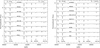 |
Fig. B.1. Optical spectra of the sequence of models calculated along the 20 M⊙ track at SMC (left) and one-thirtieth solar (right) metallicity. The main diagnostic lines are indicated at the bottom of the figure. |
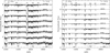 |
Fig. B.2. Ultra-violet spectra of the sequence of models calculated along the 20 M⊙ track at SMC (left) and one-thirtieth solar (right) metallicity. The main diagnostic lines are indicated at the bottom of the figure. |
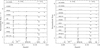 |
Fig. B.3. Infrared K-band spectra of the sequence of models calculated along the 60 M⊙ tracks at SMC (left panel) and one-thirtieth solar (right panel) metallicity. The main diagnostic lines are indicated. |
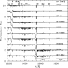 |
Fig. B.4. Ultraviolet spectra of the sequence of models calculated along the 150 M⊙ track at Z = 1/30 Z⊙. |
Appendix C: Archival data
In Table C.1 we give information on the archival spectra we used in Sect. 3.4. The data have been retrieved from the Polarbase database12, (see Donati et al. 1997; Petit et al. 2014) and the ESO phase 3 archive facility13. Spectral types are given according to the GOSS catalog (Maíz Apellániz et al. 2011, 2013).
Galactic stars for which spectra were collected from archives to measure EWs.
All Tables
Atmosphere model parameters (Teff, luminosity, surface gravity, mass-loss rate, wind terminal velocity), associated spectral types, ionizing fluxes, and EW of He II 1640 for the SMC metallicity grid.
Atmosphere model parameters (Teff, luminosity, surface gravity, mass-loss rate, wind terminal velocity), associated spectral types, ionizing fluxes and EW of He II 1640 for the Z = 1/30 Z⊙ metallicity grid.
All Figures
|
Fig. 1. Hertzsprung-Russell diagram for the Z = 1/30 Z⊙ (black lines and filled squares) and SMC (dot-dashed blue lines and open circles) cases. Lines are the STAREVOL evolutionary tracks. Symbols are the points at which an atmosphere model and synthetic spectrum have been computed. |
| In the text | |
|
Fig. 2. Optical spectra of the sequence of models calculated along the 60 M⊙ track at SMC (left) and one-thirtieth (right) metallicity from the ZAMS at the top to the post-MS at the bottom. The main diagnostic lines are indicated at the bottom of the figure. The spectra have been degraded to a spectral resolution of ∼2500, similar to that of the GOSS survey. |
| In the text | |
|
Fig. 3. Same as Fig. 2 but for the UV range. The spectra have been degraded to a spectral resolution of ∼16 000 typical of HST/COS FUV observations. |
| In the text | |
|
Fig. 4. Distribution of spectral types across the HR diagram at SMC (left panel) and one-thirtieth solar (right panel) metallicity. |
| In the text | |
|
Fig. 5. Hertzsprung-Russell diagrams at Z = 1/5 Z⊙ with the various luminosity classes indicated by symbols and colors. Top left panel: all luminosity classes, top right (respectively bottom left and bottom right) panel: focuses on dwarfs (respectively on giants and supergiants). Small open symbols are SMC stars analyzed by Mokiem et al. (2006), Bouret et al. (2013), Castro et al. (2018), Ramachandran et al. (2019) and Bouret et al. (in prep.). |
| In the text | |
|
Fig. 6. Ultra-violet spectra of the models of the Z = 1/5 Z⊙ series for which a spectral type O4V((f)) or O5V((f)) was attributed (see Table A.1). The HST/COS spectrum of the O4−5V star AzV 388 in the SMC, from Bouret et al. (2013), is inserted in red. The main lines are indicated. The initial masses of the models are also given. |
| In the text | |
|
Fig. 7. Comparison of evolutionary models without rotation at Z = 1/30 Z⊙ (our calculations in black solid lines), Z = 1/35 Z⊙ from Groh et al. (2019) (blue dashed lines), and Z = 1/50 Z⊙ from Szécsi et al. (2015) (red dotted lines). Initial masses are indicated at the beginning of each evolutionary sequence. For the Szécsi et al. (2015) 40 and 60 M⊙ tracks the actual values of the initial masses are respectively 39 and 59 M⊙. |
| In the text | |
|
Fig. 8. Hertzsprung-Russell diagram at Z = 1/30 Z⊙ with the various luminosity classes indicated by symbols and colors. |
| In the text | |
|
Fig. 9. Spectra of the sequence of models calculated along the 60 M⊙ track at SMC metallicity in the blue spectral range of ELT/HARMONI and ELT/MOSAIC. The main diagnostic lines are indicated. The spectra have been degraded to a spectral resolution of approximately 5000, which is typical of the ELT instruments. A rotational velocity of 100 km s−1 has been considered for all spectra. |
| In the text | |
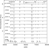 |
Fig. 10. Same as Fig. 9 but for the Z = 1/30 Z⊙ case. |
| In the text | |
|
Fig. 11. Ratio of the EW of He I 7065 to He II 5412 as a function of spectral type for the low-metallicity models calculated in the present study, the solar metallicity models of Martins & Palacios (2017) and observations of Galactic stars collected from archives (open red circles – see text for details). Left panel: all data points shown. When no unique spectral type was assigned to a model (e.g., O6−6.5) the average was used (i.e., O6.25). Numbers above ten correspond to B stars (with ten being B0, and 10.5 being B0.5). Right panel: same as left panel but showing only the average value of the EW ratio for each spectral type. In that panel the spectral types of the 1/5 Z⊙ (1/30 Z⊙) models have been shifted by +0.03 (−0.03) for clarity. We also considered only “official” spectral types, that is, we excluded for example 6.25 when a spectral type O6−6.5 was assigned to a model. |
| In the text | |
|
Fig. 12. H I ionizing fluxes per unit surface area as a function of effective temperature. Upper panel: ionizing fluxes for the two metallicities considered in this work and our solar metallicity models (Martins & Palacios 2017). Middle and bottom panel: 1/5 Z⊙ and 1/30 Z⊙ models, respectively, which are compared to TLUSTY (Lanz & Hubeny 2003) and PoWR (Hainich et al. 2019) models. |
| In the text | |
|
Fig. 13. Effect of metallicity on the SED. The initial model (red line) is the fifth model of the 60 M⊙ series at Z = 1/30 Z⊙. The blue line shows the same model for which the metallicity has been changed to 1/5 Z⊙, all other parameters being kept constant. In the model shown by the orange line, in addition to metallicity, the mass-loss rate has been increased by a factor 4.2 according to Ṁ ∝ Z0.8. Finally, in the model shown in green, the mass-loss rate has been reduced down to log Ṁ = −7.30. The H I, He I, and He II ionizing edges are indicated by vertical black lines. |
| In the text | |
|
Fig. 14. Ratio of He I (left) or He II (right) to H I ionizing fluxes as a function of effective temperature for the two metallicities considered in this work. We have also added the models of Martins & Palacios (2017) at solar metallicity. |
| In the text | |
|
Fig. 15. Same as Fig. 14 but for our SMC models (red filled triangles) and comparison models of Lanz & Hubeny (2003) (open orange circles) and Hainich et al. (2019). For the latter, cyan crosses, blue squares, and purple stars correspond to low, intermediate, and high mass-loss rates, respectively. |
| In the text | |
|
Fig. 16. HR diagram (Z = 1/5 Z⊙, left panel; Z = 1/30 Z⊙, right panel) showing the position of the models with He II 1640 emission (absorption) in black filled (open) squares. |
| In the text | |
|
Fig. 17. He II 1640 profile of the model with the strongest emission. |
| In the text | |
|
Fig. B.1. Optical spectra of the sequence of models calculated along the 20 M⊙ track at SMC (left) and one-thirtieth solar (right) metallicity. The main diagnostic lines are indicated at the bottom of the figure. |
| In the text | |
|
Fig. B.2. Ultra-violet spectra of the sequence of models calculated along the 20 M⊙ track at SMC (left) and one-thirtieth solar (right) metallicity. The main diagnostic lines are indicated at the bottom of the figure. |
| In the text | |
|
Fig. B.3. Infrared K-band spectra of the sequence of models calculated along the 60 M⊙ tracks at SMC (left panel) and one-thirtieth solar (right panel) metallicity. The main diagnostic lines are indicated. |
| In the text | |
|
Fig. B.4. Ultraviolet spectra of the sequence of models calculated along the 150 M⊙ track at Z = 1/30 Z⊙. |
| In the text | |
Current usage metrics show cumulative count of Article Views (full-text article views including HTML views, PDF and ePub downloads, according to the available data) and Abstracts Views on Vision4Press platform.
Data correspond to usage on the plateform after 2015. The current usage metrics is available 48-96 hours after online publication and is updated daily on week days.
Initial download of the metrics may take a while.