| Issue |
A&A
Volume 645, January 2021
|
|
|---|---|---|
| Article Number | A1 | |
| Number of page(s) | 15 | |
| Section | The Sun and the Heliosphere | |
| DOI | https://doi.org/10.1051/0004-6361/202038900 | |
| Published online | 21 December 2020 | |
Non-LTE inversions of a confined X2.2 flare
I. The vector magnetic field in the photosphere and chromosphere
1
Institute for Solar Physics, Department of Astronomy, Stockholm University, AlbaNova University Centre, 106 91 Stockholm, Sweden
e-mail: This email address is being protected from spambots. You need JavaScript enabled to view it.
2
Astrophysics Research Centre, School of Mathematics and Physics, Queen’s University Belfast, BT7 1NN Belfast, Northern Ireland, UK
3
Department of Physics, University of Helsinki, PO Box 64 00014 Helsinki, Finland
4
Institute for Space-Earth Environmental Research (ISEE), Nagoya University Furo-cho, Chikusa-ku, Nagoya 464-8601, Japan
Received:
13
July
2020
Accepted:
8
September
2020
Abstract
Context. Obtaining an accurate measurement of magnetic field vector in the solar atmosphere is essential for studying changes in field topology during flares and reliably modelling space weather.
Aims. We tackle this problem by applying various inversion methods to a confined X2.2 flare that occurred in NOAA AR 12673 on 6 September 2017 and comparing the photospheric and chromospheric magnetic field vector with the results of two numerical models of this event.
Methods. We obtained the photospheric magnetic field from Milne-Eddington and (non-)local thermal equilibrium (non-LTE) inversions of Hinode SOT/SP Fe I 6301.5 Å and 6302.5 Å. The chromospheric field was obtained from a spatially regularised weak-field approximation (WFA) and non-LTE inversions of Ca II 8542 Å observed with CRISP at the Swedish 1 m Solar Telescope. We investigated the field strengths and photosphere-to-chromosphere shear in the field vector.
Results. The LTE- and non-LTE-inferred photospheric magnetic field components are strongly correlated across several optical depths in the atmosphere, with a tendency towards a stronger field and higher temperatures in the non-LTE inversions. For the chromospheric field, the non-LTE inversions correlate well with the spatially regularised WFA, especially in terms of the line-of-sight field strength and field vector orientation. The photosphere exhibits coherent strong-field patches of over 4.5 kG, co-located with similar concentrations exceeding 3 kG in the chromosphere. The obtained field strengths are up to two to three times higher than in the numerical models, while the photosphere-to-chromosphere shear close to the polarity inversion line is more concentrated and structured.
Conclusions. In the photosphere, the assumption of LTE for Fe I line formation does not yield significantly different magnetic field results in comparison to the non-LTE case, while Milne-Eddington inversions fail to reproduce the magnetic field vector orientation where Fe I is in emission. In the chromosphere, the non-LTE-inferred field is excellently approximated by the spatially regularised WFA. Our inversions confirm the locations of flux rope footpoints that have been predicted by numerical models. However, pre-processing and lower spatial resolution lead to weaker and smoother field in the models than what our data indicate. This highlights the need for higher spatial resolution in the models to better constrain pre-eruptive flux ropes.
Key words: Sun: chromosphere / Sun: photosphere / Sun: flares / Sun: magnetic fields / radiative transfer
© ESO 2020
1. Introduction
Flares and coronal mass ejections (CMEs) are a source of the most violent heliospheric disruptions and understanding what triggers them is an essential piece in the space weather puzzle. To reliably predict either is not a straightforward exercise, however. Current forecasting efforts build on the round-the-clock coverage of the Earth-facing side of the Sun, carried out by the Solar Dynamics Observatory (SDO; Pesnell et al. 2012), which provides a view from the photosphere to the corona in the (extreme) ultraviolet, along with photospheric magnetic field information from the Fe I 6173 Å line. Such data allow for a parametrisation of the photospheric field over large regions, using properties of the polarity inversion line (Schrijver 2007), connectivity across it (Georgoulis & Rust 2007), and amount of magnetic shear or helicity (e.g. Kusano et al. 2012; Pariat et al. 2017; Zuccarello et al. 2018) that are known to be indicators of an active region’s eruptive potential. These properties have been used individually or combined with the SDO’s upper-atmosphere diagnostics to arrive at a prediction through either statistical models or machine-learning techniques, which have become increasingly popular over the past few years (e.g. Leka & Barnes 2003, 2007; Bobra & Couvidat 2015; McCloskey et al. 2016; Florios et al. 2018; Jonas et al. 2018; Nishizuka et al. 2018; Panos & Kleint 2020).
Still, this means that it is usually only the lower magnetic (or the derived electric) field boundary conditions that are taken into account, while neglecting the chromospheric magnetic field vector. Including the latter, on the other hand, could significantly aid data-driven modelling (e.g. De Rosa et al. 2009; Toriumi et al. 2020) of, for instance, the magnetic field structure of CMEs (Kilpua et al. 2019), which is, in turn, important for space weather forecasts. An important obstacle here is that the necessary spectropolarimetric observations are neither widely nor commonly acquired and when they are, the field of view is typically limited. Consequently, flare studies that include chromospheric polarimetry (and do so at high spatial resolution) are sparse (e.g. Sasso et al. 2014; Kuckein et al. 2015; Judge et al. 2015; Kleint 2017; Kuridze et al. 2018, 2019; Libbrecht et al. 2019).
Towards the end of the last Solar Cycle 24, the NOAA active region (AR) 12673 evolved from a lonely symmetric sunspot, as it appeared when rotating into view, into an active and complex sunspot group by the time it crossed the central meridian. The flaring activity of this active region has been studied extensively over the past two years, especially given that over the span of a week it produced four X-class flares, including the two largest flares of that cycle (X9.3 on September 6 11:53 UT and X8.2 on September 10 15:35 UT), along with over two dozen M-class flares and many more smaller ones. Moreover, the X9.3 flare was preceded by a confined X2.2 flare a mere 3 h earlier. The active region developed as flux that emerged, over the course of three days, next to an α-class sunspot coalesced and led to a complex δ-spot configuration, where strong shearing flows along the polarity inversion line (PIL) between the positive-polarity spot and parasitic negative polarity were likely the main agent in setting up the active region for flaring (Yang et al. 2017; Romano et al. 2018; Wang et al. 2018a; Verma 2018).
Given the near-continuous coverage by the Helioseismic and Magnetic Imager (HMI; Scherrer et al. 2012; Schou et al. 2012) aboard SDO combined with the availability of its derived data products such as Spaceweather HMI Active Region Patches (SHARPs; Bobra et al. 2014), also renders this an attractive target in the study of the magnetic field configuration and evolution during emergence and flaring. For instance, Hou et al. (2018) focussed on the two largest flares that the active region has brought forth (i.e. the X9.3 and X8.2 flares), using a time sequence of non-linear force free field (NLFFF) extrapolations to investigate the field evolution during the flares. For both flares they found a multi-flux-rope configuration over the PIL, wherein the flux ropes were destabilised by the shearing and rotating motions of the δ-sunspot, setting off the upper flux rope and leading to the destabilisation of adjacent flux ropes that ended up erupting shortly after. Following a similar approach, Liu et al. (2018a) used a time series of NLFFF and potential field models to study the confined X2.2 flare that preceded the X9.3 one. They also identified a multiple-branch or double-decker magnetic flux rope configuration. During the confined flare, the magnetic helicity was found to increase by over 250% from pre-flare values and became again significantly reduced during the subsequent X9.3 flare, implying a scenario in which the confined flare set the stage for the eruptive one. Zou et al. (2019), analysing a series of NLFFF extrapolations obtained using a magnetohydrodynamic (MHD) relaxation method, suggested a two-step reconnection process in which reconnection first occurred in a null point outside the magnetic flux rope system and at around 4000 km height, while the associated disturbance then triggered the second, tether-cutting reconnection. However, as the overlying field was sufficiently strong, the flare remained confined. Romano et al. (2019) performed NLFFF extrapolations as well and identified null points for the X2.2 and X9.3 flares at 5000 and 3000 km above the photospheric boundary, respectively.
More elaborate modelling set-ups were performed by Inoue et al. (2018), Jiang et al. (2018), and Price et al. (2019). In the first study, the authors performed a MHD simulation for which the initial magnetic configuration was set by a NLFFF extrapolation from a SHARP about 20 min prior to the X2.2 flare. Their results suggest that the X2.2 flare may have been associated with the rise of a small flux rope, triggered by reconnection underneath it, and that the X9.3 flare was likely to be the eruption of a large-scale magnetic flux rope that had been formed through reconnection between several smaller ones in the hours leading up to the large flare. Similarly, Jiang et al. (2018), analysed a NLFFF extrapolation-initialised MHD simulation of the X9.3 flare and identified tether-cutting reconnection as the likely trigger of the flux rope eruption. On the other hand, Price et al. (2019) performed time-dependent magnetofrictional modelling to investigate the emergence and evolution that led up the X9.3 flare and associated eruption and coronal mass ejection. As such, their simulation covers also the preceding confined X2.2 flare. Feeding the model with a time series of electric field inversions based on the SDO/HMI vector magnetic field, with the magnetic field initialised from a potential field extrapolation, the authors report an increase in helicity during the X2.2 flare consistent with the findings of Liu et al. (2018a) and while the magnetic flux rope did not erupt out of the simulation’s numerical domain during the X9.3 flare, in contrast to the results by Inoue et al. (2018), both studies produce a similar large-scale field configuration and evolution, as well as structure of the erupting flux rope.
However, a limitation of all the field extrapolation and modelling efforts mentioned above is the lack of chromospheric magnetic field input. Including chromospheric field information has been shown to aid the NLFFF extrapolation in recovering the chromospheric and coronal magnetic field structure (Fleishman et al. 2019). Similarly, Toriumi et al. (2020) compared several data-driven model results based on a flux emergence simulation and found that the largest errors were due to strong Lorentz forces at the photospheric boundary inducing spurious flows that altered the magnetic field (via the induction equation), whereas the inclusion of the field at a higher, and much more force-free, layer resulted in better agreement with the input simulation. While the (non-magnetic) Hα response to the X9.3 flare has been studied in detail in Quinn et al. (2019), the chromospheric magnetic field of neither of the 6 September flares has previously been investigated based on observations.
We take on part of that challenge in the present study and focus on the confined X2.2 flare in NOAA AR 12673 for which high-resolution observations of both photospheric and chromospheric spectropolarimetry are available. Section 2 introduces the observations and post-processing to prepare the data for inversions. Section 3 describes different approaches we employed in inferring the photospheric and chromospheric magnetic field vectors, with Sect. 4 presenting our results. We also compare those against two numerical models in Sect. 5. We discuss our findings in Sect. 6 and present our conclusions in Sect. 7.
2. Observations and reduction
We analysed a confined X2.2 flare in NOAA AR 12673 on 6 September 2017 that lasted from 08:57 to 09:17 UT, peaking at 09:10 UT. Part of its rise and decay phase was observed by the Solar Optical Telescope (SOT; Tsuneta et al. 2008) Stokes Spectro-Polarimeter (SP) aboard Hinode (Kosugi et al. 2007), as well as the CRisp Imaging SpectroPolarimeter (CRISP; Scharmer et al. 2008) at the Swedish 1 m Solar Telescope (SST; Scharmer et al. 2003). Figure 1 presents an overview of these observations, along with contextual line-of-sight (LOS) magnetic field from a SDO/HMI-derived SHARP two minutes after the flare peak.
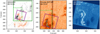 |
Fig. 1. Overview of the analysed data, showing the SDO/HMI-derived SHARP LOS magnetic field from Fe I 6173 Å (left), Hinode/SP continuum near Fe I 6302 Å (middle) and SST/CRISP Ca II 8542 Å red wing at +0.5 Å (right). The Hinode and SST fields of view are indicated in the first two panels with green and purple boxes, respectively, while the dashed light green box in the first two panels outlines the cut-out of Fig. 2. The cyan contours in the middle panel indicate locations where the Fe I lines are in emission. Times in UT are indicated in the top left of each panel (for Hinode SOT/SP the time corresponds to the middle of the slit raster-scan). The vertical stripes in the middle panel are due to missing data. |
Imaging spectropolarimetry in the Ca II 8542 Å line was obtained at the SST between 09:04:30 and 09:54:24 UT, sampling 11 wavelength positions out to ±0.7 Å from line centre (at 0.1 Å spacing between ±0.3 Å and at 0.2 Å in the wings) at an overall cadence of 15 s per scan. The pixel scale is  pix−1. The data were reduced with the CRISPRED (de la Cruz Rodríguez et al. 2015) pipeline, including image restoration using Multi-Object Multi-Frame Blind Deconvolution (MOMFBD; van Noort et al. 2005), along with the removal of remaining small-scale seeing-induced deformations (Henriques 2012) and destretching to correct for rubber-sheet seeing effects (Shine et al. 1994).
Additional treatment of the data was necessary to increase the signal-to-noise in Ca II 8542 Å Stokes Q and U, and we applied the denoising neural network of Díaz Baso et al. (2019), followed by Fourier-filtering to suppress the strongest remaining high-frequency fringe patterns (similar to the method described in Pietrow et al. 2020). As the seeing conditions were variable at La Palma, we selected a single line scan snapshot at 09:09:00 UT for further study, based on best contrast throughout the line scan and fortuitously close in time to the flare peak.
Hinode SOT/SP performed a fast map of 164″ × 164″ full spectropolarimetry in Fe I 6301.5 Å and 6302.5 Å at 3.2 s integration time per slit position between 09:03:40 and 09:27:53 UT, resulting in a mid raster-scan time of 09:15:47 UT. The raster pixel size is  . For the sub-field cutout marked by the dashed box in Fig. 1, the mid-scan time is 09:09:14 UT, close to the selected best-contrast frame of the SST data set and the flare peak. We did not attempt simultaneous inversion of the Hinode and SST data, as SOT/SP required nearly 11 min to scan the sub-field, leading to increasingly inconsistent Fe I and Ca II profiles towards the vertical edges of the overlapping field of view (FOV). However, the SOT/SP sampling of the polarity inversion line vicinity, which is what we are primarily interested in, falls within 3 min of the Ca II line scan snapshot.
Data alignment. We aligned the SST data to Hinode through cross-correlation, using the Hinode continuum image (Fig. 1, middle panel) as anchor to which the Ca II 8542 Å wide-band image was aligned. This includes downsampling the SST data to Hinode resolution (about a factor of five in both x and y) as part of the alignment process. As we are primarily interested in comparing the photospheric and chromospheric field in the same pixels, this is a reasonable compromise to make and it has the added benefit of saving computational time, as well as improving the S/N of the polarimetric data. CRISPEX (Vissers & Rouppe van der Voort 2012; Löfdahl et al. 2018) was used to verify inter-instrument alignment and for data browsing.
3. Methods for magnetic field vector inference
Several methods exist for inferring or deriving the magnetic field vector from observations, varying in the degree of complexity and computational expense. In this section, we discuss the three methods used in this study. On one hand, we use Milne-Eddington inversions and a spatially regularised weak-field approximation that provide a field estimate under simplifying assumptions. On the other hand, we employ (non-)LTE inversions that yield a depth-stratified model atmosphere with temperature, velocities, and magnetic field, albeit at higher computational cost.
3.1. Milne-Eddington inversions
As an approximation of the photospheric field, we use the pixel-by-pixel (i.e. each pixel is treated independently) Milne-Eddington (ME) inversion results obtained with the Milne-Eddington gRid Linear Inversion Network (MERLIN) code. These inversions are performed assuming a source function that is linear with optical depth, but where such quantities as the magnetic field vector and LOS velocity are otherwise constant throughout the atmosphere. We also note that in the routine application of the MERLIN code a saturation limit of 5 kG is imposed on the LOS and horizontal field strengths. The SOT/SP level-2 data product readily delivers these results and contains (among other quantities) the field strength value, its inclination, and azimuth, where the latter still has an unresolved 180° ambiguity. We discuss our disambiguation approach for this and the other inferred azimuths in Sect. 3.4.
3.2. Spatially regularised weak-field approximation
An estimate of the chromospheric magnetic field can be obtained using the weak-field approximation (WFA, Landi Degl’Innocenti 1992; Landi Degl’Innocenti & Landolfi 2004), which assumes that the Zeeman splitting is smaller than the Doppler broadening of the line in question. This method does not bear the cost of solving the full non-LTE radiative transfer problem and lends itself well, therefore, to a fast estimation of the magnetic field over a larger field of view, but at the same time, it suffers from several simplifications and a limited range of validity that need be borne in mind (Centeno 2018). The WFA has found its use for targets like sunspots (de la Cruz Rodríguez et al. 2013), plage (Pietarila et al. 2007), as well as in flares (Harvey 2012; Kleint 2017).
Here we use a spatially regularised WFA (Morosin et al. 2020), namely, an extension of the commonly used pixel-by-pixel one, to infer the approximate chromospheric magnetic field configuration over the full SST FOV. The spatially regularised approach departs from the idea that when the observations are properly sampled near the diffraction limit of the telescope, the derived magnetic field should be spatially smooth in its variation. The implementation we use employs Tikhonov ℓ-2 regularisation and to impose the smoothness, the values of the four nearest-neighbours (±1 pixel in both the x- and y-direction) are taken into account when minimising χ2. The power of this method is that with well-chosen parameters the effects of noise can be drastically mitigated. For further details we refer to Morosin et al. (2020).
Finally, we note that we obtained the weak-field approximation results (including azimuth disambiguation) before downsampling to Hinode resolution was performed as part of the data alignment process.
3.3. Non-LTE inversions
We used the STockholm Inversion Code (STiC; de la Cruz Rodríguez et al. 2016, 2019) to infer the atmospheric stratification of temperature, velocities, and magnetic field from the Hinode Fe I and SST Ca II data. The STiC is an MPI-parallel non-LTE inversion code built around a modified version of RH (Uitenbroek 2001) to solve the atom population densities assuming statistical equilibrium and plane-parallel geometry, using an equation of state extracted from the SME code (Piskunov & Valenti 2017). We assumed complete frequency redistribution (CRD) in our inversions. The radiative transport equation is solved using cubic Bezier solvers (de la Cruz Rodríguez & Piskunov 2013). As the Hinode SOT/SP scanning time was too long to obtain consistent Fe I and Ca II profiles for the overlapping part of the FOV, we decided to perform the inversions for both lines separately and, therefore, we could not take advantage of the multi-resolution inversion technique recently proposed by de la Cruz Rodríguez (2019).
The Ca II inversions were performed in non-LTE using a six-level calcium model atom and assuming CRD. For Fe I we performed both LTE and non-LTE inversions, spurred in part by the recent study by Smitha et al. (2020). They report on LTE inversions of Fe I 6301 Å and 6302 Å that were synthesised assuming either LTE or non-LTE, which indicate that LTE inversions of non-LTE Fe I may result in discrepancies with the input model in terms of temperature (of order 10%) and LOS velocities and magnetic field (both up to 50%), while the field inclination could exhibit errors of up to 45°. For both the LTE and non-LTE Fe I inversions we used the same extended 23-level Fe I atom that has been used in several studies on the non-LTE radiative transfer effects in the Fe I lines over the past decade (Holzreuter & Solanki 2013, 2015; Smitha et al. 2020).
As initial input atmosphere we used a FAL-C model interpolated to a Δlog τ500 = 0.2 grid between log τ500 = −8.5 and 0.1, but truncated at log τ500 = −5 (i.e. excluding the upper atmosphere) for Fe I given the lack of sensitivity of the line to conditions much above the temperature minimum. Both the Fe I and Ca II inversions were performed in two cycles with spatial and depth smoothing of the model atmosphere between the first and second cycle, as well as an increased number of nodes in temperature, velocity, and magnetic field component in the second cycle (see Table 1). In addition, as the flaring emission profiles in both Fe I and Ca II proved a challenge for the first cycle inversions, we replaced the atmospheres of the worst fitted pixels (as expressed by their χ2-value) with the average atmosphere of nearby well-fitted pixels with same-sign LOS field prior to smoothing for the second cycle input. The results of these inversions are presented in Sect. 4.
Number of nodes used in each inversion cycle.
3.4. Azimuth disambiguation
The photospheric and chromospheric magnetic field azimuth φ recovered from both the Milne-Eddington inversions, the weak-field approximation, and STiC inversions contain a 180° ambiguity that needs to be resolved for proper interpretation of the horizontal magnetic field component. Several schemes exist for this disambiguation (Metcalf et al. 2006); here we use the implementation by Leka et al. (2014) of the minimum energy method (MEM) proposed by Metcalf (1994), which simultaneously minimises the divergence of the field and the current density. This method works well for photospheric lines, where the linear polarisation signal is sufficiently strong, but the method typically struggles for Ca II 8542 Å where the Stokes Q and U profiles are noisier. Above the sunspot and during the flare, however, the linear polarisation signal is sufficiently strong that the azimuth can be reliably recovered in the chromosphere. In order to check what areas of the FOV are uncertain for the ambiguity resolution, we ran the MEM code with twenty different random number seeds. Regions where the azimuth result changed by more than 45° between runs were considered to be unstable for disambiguation and for those pixels we set the azimuth by majority vote of the results from the twenty realisations.
4. Observationally inferred magnetic field vector
4.1. LTE versus non-LTE inversions of Fe I
Figures 2–4 compare the results from the STiC LTE and non-LTE inversions of the Fe I 6301.5 Å and 6302.5 Å spectra. Figure 2 shows the photospheric LOS magnetic field with arrows indicating the magnetic field azimuth where their hue reflects the horizontal field strength (i.e. darker blue being stronger). Qualitatively, the LTE and non-LTE inversions of Fe I yield very similar magnetic field distributions, especially at log τ500 = −0.5 and −1.1. Also the field azimuth shows largely the same pattern, much as the strong horizontal field distribution (bright green contours for Bhor > 5 kG) does to a certain extent. Where the field is weak (both LOS and horizontal, e.g. in the top left part of the FOV), the azimuth displays apparently random orientations, contrasting with the more ordered pattern in the strong-field sunspot umbra and penumbra, even though the distinct “whirlpool-like” pattern in the “head” of the inverse-S shaped polarity inversion line (i.e. around (X, Y) = (510″, −235″)) is only recovered with the non-LTE inversions. Regardless of LTE or non-LTE, the azimuth is essentially parallel to the PIL in its vicinity, except in the positive-polarity umbra around (X, Y) = (515″, −245″). The largest differences are primarily found at and close to the locations where the Fe I lines go into emission, highlighted by the cyan contours in the first column. While both inversions yield negative polarity in the cyan-outlined “head” of the inverse-S and positive polarity in the western umbra, this only persists at all three shown log τ500-depths for the LTE inversion (albeit no longer as smoothly at log τ500 = −2.1), while for the non-LTE inversion opposite polarity starts appearing around (X, Y) = (515″, −255″) at log τ500 = −1.1 and −2.1.
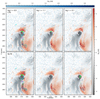 |
Fig. 2. Line of sight and transverse magnetic field from STiC (non-)LTE inversions of the Fe I Hinode data over the sub-field indicated by the dashed green box in Fig. 1. From left to right the columns show the photospheric field at different log τ500 depths as specified in the top left corner of each panel, both for LTE (top row) and non-LTE (bottom row) inversions. The maps are of the LOS field (scaled according to the right-hand colour bar), while the blue arrows indicate the azimuth direction, where their hue reflects the horizontal field strength (according to the top colour bar). All panels are colour-scaled between the same values with both LOS and horizontal field strengths clipped to the range wherein 98% of the pixels fall. Bright green contours indicate where the horizontal field is in excess of 5 kG, while the cyan contours in the first column highlight where the Fe I lines are in emission. The coloured plus signs mark the locations for which (non-)LTE profile fits are shown in Fig. 4. |
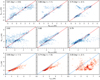 |
Fig. 3. Two-dimensional histograms of non-LTE versus LTE LOS magnetic field strength (top row), horizontal field strength (middle row), and temperature (bottom row) for the flaring pixels (i.e. within cyan contours in Fig. 2) at three log τ500 depths. The Pearson correlation number is shown in the top left of each panel and the log τ500 depth within parenthesis in the top row panels (for magnetic field) and bottom row panels (for temperature), while the straight lines indicate what would be linear relationship. |
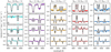 |
Fig. 4. Fe I 6301.5 Å and 6302.5 Å profiles from observations and (non-)LTE inversions. Each column shows (from top to bottom) Stokes I, Q, U and V profiles as observed (coloured dots) and as fitted in LTE (grey dashed line) and in non-LTE (solid black line). The colour coding corresponds to the identically coloured plus markers in the left-hand panels of Fig. 2. The numbers above each column indicate the non-LTE-inferred Blos and Bhor at log τ500 = −0.5. |
Figure 3 quantifies this behaviour through two-dimensional (2D) histograms of the LOS and horizontal field, as well as the temperatures for pixels where Fe I is in emission. As the magnetic field scatter plots (top two rows) show, the correlation is overall positive for Blos and Bhor and relatively tight for the former, especially around log τ500 = −1.1, even though there is a cloud of points at negative Blos, NLTE and positive Blos, LTE at all three log τ500-depths. Upon closer inspection, these turn out to be scattered pixels in the emission patches around Y = −250″ for which negative Blos was inferred in non-LTE. These panels also evidence that, while in general neither Blos nor Bhor exceed 3 kG by much (cf. also the colour bars in Fig. 2, clipped to the range wherein 98% of the pixels fall), there are pixels where values of 4−6 kG are reached for either field component. Many pixels are also inverted with somewhat lower LOS field strength in LTE than in non-LTE (cf. the scatter clouds above the diagonal line at negative Blos, NLTE and below at positive Blos, NLTE for log τ500 = −0.5 and −1.1). The opposite appears true at log τ500 = −2.1 (top right panel). The median fractional difference (Blos, NLTE − Blos, LTE)/Blos, LTE reaches up to 6.7% at log τ500 = −0.5, but decreases to −2.1% at log τ500 = −2.1, while for the full FOV, it peaks to 9.1% at log τ500 = −1.1. On the other hand, for the horizontal field the LTE-inferred Bhor is typically stronger than in the non-LTE inversion, in particular, at low and middle log τ500-depths (median fractional difference of around −7%), while at log τ500 = −2.1 pixels can be found above 4 kG in non-LTE that barely reach that value in the LTE inversion.
The discrepancies are even larger with regard to temperature (bottom row of Fig. 3), with a strong correlation between LTE and non-LTE-inferred temperatures at log τ500 = −0.5, but an increasingly loose scatter higher in the atmosphere at log τ500 = −1.5 and especially −2.1. At those heights, fewer and fewer pixels lie on the diagonal and there is a clear tendency for higher temperatures in non-LTE, inferring some 7−8 kK versus 4−5 kK in LTE. The median non-LTE-to-LTE fractional difference increases from 1.5% at log τ500 = −0.5 to nearly 25% at log τ500 = −2.1 for the flaring pixels. For the full FOV, that difference reaches 5.6% at the same height.
Finally, Fig. 4 presents several examples of observed profiles and LTE and non-LTE fits to those – one from a magnetic concentration outside the sunspot and four from the (vicinity of the) flare. Striking for some of the latter is the evident Zeeman splitting in Fe I 6302.5 Å Stokes I, suggesting strong magnetic fields. As these panels show, we find only very minor differences between the LTE and non-LTE fits, regardless of the profile shape. In the “quiet Sun” sampling (first column) the 6301.5 Å Stokes Q is better fitted in LTE, while the non-LTE fit to 6302.5 Å gets closer to the observations. The PIL-sampling (second column) is similarly fitted in either approach, but it is, in fact, possible to fit the flaring emission profiles (last three columns) even in LTE, with little difference compared to non-LTE. The Stokes V is especially well-fitted in these cases and both LTE and non-LTE sometimes struggle in reaching the extrema (e.g. 6302.5 Å Stokes U in the middle sampling (orange) or 6301.5 Å Stokes Q in the last (blue) one). Either way, the outer wings of the Fe I lines in Stokes I generally prove to be challenging to fit simultaneously with the emission peaks, where the LTE fit is marginally closer (yet still not close) to the observations.
4.2. Milne-Eddington and weak-field approximation versus non-LTE inversions
Photospheric field. Figure 5 compares the Milne-Eddington photospheric and weak-field approximation chromospheric fields (left panels a and d) with their equivalents from non-LTE inversions (middle panels b and e). We first consider the photospheric field (bottom panels d and e). A limitation inherent to the Milne-Eddington inversions is that a linear source function cannot simultaneously explain absorption and emission features. Considering that in the places where the Fe I cores are in emission, the wings generally exhibit absorption dips (cf. Fig. 4), thus, the Milne-Eddington inversion will likely fit the wings under the assumption that the polarity reversal in Stokes V is due to a change in the sign of the LOS magnetic field, rather than a change in slope of the source function. This explains the evident discrepancy in LOS magnetic field where the Fe I lines are in emission (black contours). While the Milne-Eddington inversion returns an embedded opposite polarity in those areas, the non-LTE inversion yields same-sign LOS field that corresponds to the dominant polarity in either umbra of the δ-spot. Similarly, this is likely to explain the discrepancy in azimuth direction for those pixels. Finally, the previously noted MERLIN saturation limit of 5 kG means that the strong LOS and horizontal field that were inferred in both the LTE and non-LTE inversions (see Figs. 2 and 3) cannot be reproduced with the Milne-Eddington approach, where the LOS field ranges from −3.6 kG to saturation at +5 kG, also reaching saturation for the horizontal field.
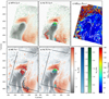 |
Fig. 5. Chromospheric and photospheric magnetic field from the inversion methods that we applied. Panel a: chromospheric LOS field maps with green azimuth arrows coloured according to its horizontal field strength from the spatially regularised WFA. Panel b: same as panel a but from STiC non-LTE inversions. The contours mark where the field exceeds 4.5 kG in the photosphere and 3 kG in the chromosphere for Blos (cyan) and the same thresholds for Bhor (light green). The coloured plus markers indicate the locations for which Fig. 7 shows Ca II 8542 Å profile fits. Panel c: angle difference θ(BWFA, BSTiC) between the WFA and non-LTE three-dimensional (3D) field vectors, clipped to 100°. The dashed white contours highlight the regions where the WFA field strength exceeds 2 kG (selected pixels for Fig. 6). Panel d: photospheric LOS field maps with blue azimuth arrows as derived in the Milne-Eddington inversion. The black box indicates the SST FOV, while the contours highlight where the Fe I lines are in emission. Panel e: same as panel d but from the non-LTE inversions and contours as in panel b. The colour bars in the lower right are for the LOS field (grey-white-red), horizontal field in the photosphere (blue) and chromosphere (green), and the angle θ (rainbow). The colour bar range for the magnetic field strengths is representative of 98% of the pixels (as in Fig. 2). |
Chromospheric field. As the non-LTE inversions yield a depth-stratified atmosphere, we investigate the response of the Ca II Stokes profiles to magnetic field changes and find that this response peaks somewhere between log τ500 = −2.7 and −4.3 depending on the pixel in question. Hence, we decided to average the magnetic field components over seven depth points centred at log τ500 = −3.5, effectively covering log τ500 = [ − 2.9, −4.1].
The chromospheric LOS field maps from the weak-field approximation (Fig. 5a) and non-LTE inversions (Fig. 5b) are largely the same, both in the distribution of opposite polarities and in the strengths that they reach. The evident exception is a band of positive polarity around (X, Y) = (500″, −250″) in the non-LTE results, where the solution may have converged to a local minimum and failed to fit all four Stokes parameters as well as it did outside this band. In addition, the non-LTE inversion exhibits stronger field both below and above the “head” of the inverse-S polarity inversion line, compared to the WFA map. The latter is naturally smoother given the spatial regularisation that couples the solution from neighbouring pixels.
Considering then the horizontal field (green arrows) from the spatially regularised weak-field approximation (Fig. 5a) and non-LTE-inferred results (Fig. 5b), and comparing with that in the photosphere, we find that in both cases, for most of the positive polarity (right of X = 510″) and part of the negative polarity (between X = 510″ and 515″), the photospheric and chromospheric field azimuth point in nearly the same direction. Unsurprisingly, the discrepancies are larger in the top left of the SST FOV (black box in the lower panels), as the field is weaker there, but also close to the polarity inversion line for the ME–WFA comparison, while the non-LTE-inferred azimuths are in closer agreement between the photosphere and chromosphere.
In comparing the chromospheric field from the WFA and non-LTE inversions, we also see that in both the horizontal component has a similar orientation in the vicinity of the polarity inversion line and in strong LOS field areas in general. This similarity holds also for the 3D magnetic field vector, as visualised in Fig. 5c, mapping the angle difference θ between the non-LTE-inferred and WFA-derived magnetic field vectors. This angle θ is obtained simply as
 (1)
(1)
where in this case B1 = BWFA and B2 = BSTiC. Over the full FOV, more than 75% of the pixels have an angle of 55° or less, but this statistic is in part driven by the large angle differences that are found in weak-field regions (top left corner), where the derivation of the azimuth is not as reliable. In the strong-field parts of the FOV, θ < 15° in general, with the exception of the band of large θ around (X, Y) = (500″, −250″), where the non-LTE inversion (erroneously) returns a positive Blos value.
Figure 6 quantifies the degree of similarity further and presents 2D histograms for the LOS and horizontal field components, as well as the distributions of the angle θ between the two 3D magnetic field vectors and the field inclination as derived with either method. In all three panels, results are shown for those pixels for which the total WFA magnetic field strength (|BWFA|) exceeds 2 kG (white contours in Fig. 5c). From the left-hand and middle panels we see that the WFA LOS magnetic field strength is strongly correlated with that of the non-LTE inversions, but we also see that the horizontal field strength presents a wide scatter cloud. About 45% of the selected pixels have a stronger LOS component in the non-LTE inversions than in the WFA, but slightly more than half have a higher horizontal field (53%) and total field (54%) strength when inferred with STiC. The median non-LTE-to-WFA fractional difference is only a few percent for either component: 1.2% for Blos, 3.0% for Bhor, and 2.0% for Btot. In addition, two features stand out: firstly, the LOS panel indicates a higher density on the diagonal at roughly ±2 kG, but these disappear when taking all pixels into account and they are therefore a visualisation artefact from excluding pixels with |BWFA| < 2 kG; secondly, the roughly horizontal scatter around Blos, WFA = −2 kG and extending over all positive Blos, STiC values is due to pixels that have erroneously been inferred with positive LOS field strengths in the latter (cf. Fig. 5b and the aforementioned band of large θ around (X, Y) = (500″, −250″) in Fig. 5c).
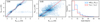 |
Fig. 6. 2D histograms of non-LTE versus WFA LOS magnetic field strength (left), horizontal field strength (middle) and histograms of angle differences (right) between the 3D field vector as recovered from the WFA and non-LTE STiC inversions (solid blue) and between their field inclinations γWFA and γSTiC (dashed red) for pixels where the total WFA magnetic field strength exceeds 2 kG (white contours in Fig. 5d). Format for the left two panels as in Fig. 3. |
The right-hand panel shows that the distribution of angles θ between the 3D magnetic field vectors (solid blue line) is skewed to smaller angles. The distribution has a median of 8° and over 91% of the pixels have an angle between the WFA and non-LTE-inferred magnetic field vectors of 25° or less. Only 4% of the pixels has an angle larger than 50° (i.e. outside the panel’s range). The absolute difference between the WFA- and non-LTE-inferred field inclinations (|γWFA − γSTiC|, dashed red line) is equally skewed, with a median of 5° and over 90% of the pixels with an inclination difference of less than 15°. Hence, although the horizontal field strengths are not as tightly correlated, the per-pixel magnetic field orientation is very similar between the WFA and non-LTE inversion.
Finally, Fig. 7 presents a selection of Ca II 8542 Å profile fits for the coloured markers in Fig. 5b. The first column samples a pixel in the positive-polarity umbra, while the other four are of pixels in the Ca II flare ribbons, where the last two are for the same red and blue pixels as in Fig. 4. The complex umbral profile (cyan) is well-fitted in all four Stokes components, except for a spurious local maximum in Stokes Q. Overall, the fits to Stokes I and V follow the observations closely regardless of the intensities and profile shapes, while Stokes Q and U sometimes prove more difficult (e.g. purple and blue samplings, in particular the blue Stokes U), despite the high S/N. Systematic errors (e.g. calibration errors due to remaining fringes or variable seeing) in combination with a typically weaker signal compared to Stokes V are likely culprits for such occasionally poorer fits to Stokes Q and/or U. The stronger horizontal chromospheric fields are in general only inferred when Stokes Q and U are both well-recovered (e.g. orange and red samplings). In some cases (e.g. blue), the strong LOS field leads to visibly Zeeman-splitted Stokes V lobes.
 |
Fig. 7. Ca II 8542 Å profiles from observations and non-LTE inversions for the coloured plus markers in Fig. 5b. Format as for Fig. 4, except that only non-LTE fitted profiles are shown (solid grey). The numbers above each column indicate the inferred Blos and Bhor averaged over log τ500 = [ − 2.9, −4.1]. |
Magnetic field strengths. While most of the FOV is inferred with relatively common field strengths of up 2−3 kG in the photosphere and slightly lower in the chromosphere (cf. the colour bars in Figs. 2 and 5), certain pixels are inferred with values well in excess of that. These are typically found for flaring profiles in Fe I and Ca II and some examples are given in Fig. 4 (last three columns) where |Btot| ≃ 5.5−6 kG in the photosphere. However, the contours in the middle panels of Fig. 5, outlining places where the photospheric field exceeds 4.5 kG and the chromospheric field 3 kG in Blos (cyan) and the same thresholds in Bhor (green), show that these typically are not isolated pixels. Moreover, while these are somewhat arbitrary thresholds, changing their values does not change the fact that this strong field is generally clustered in coherent patches that persist from photosphere to chromosphere.
5. Comparison with numerical models
We compare our magnetic field inference results with those from two numerical simulations, namely the magnetofrictional (MF) model from Price et al. (2019; see also details in Pomoell et al. 2019) that was driven time-dependently with the inferred electric field (Lumme et al. 2017) from HMI vector magnetic field data, as well as the magnetohydrodynamic model by Inoue et al. (2018) that was initialised on a NLFFF extrapolation of the HMI photospheric field at 08:36 UT. For the former, we consider the model snapshot at 09:24 UT, which is the one closest in time to the X2.2 flare peak, while for the latter, we take the model snapshot at t = 0.28 h, equivalent to 08:52:48 UT (just 4 min before the X2.2 flare). This choice is constrained by the cadence of the respective simulations and our aim to compare with the observationally inferred field. Furthermore, we note that selecting a different snapshot from the magnetofrictional model would not significantly alter our comparison or conclusions given the temporal smoothing applied in its pre-processing (see discussion in Sect. 6.4).
For both simulations, we take the photospheric field from the z = 0 Mm height, while we consider the average Ca II 8542 Å formation height in our FOV to be between 1 and 2 Mm (cf. e.g. Bjørgen et al. 2019) and select the only height index that falls in that range in both simulations, resulting in z = 1.75 Mm for the MF model and z = 1.44 Mm for the MHD model. This choice is again a limitation imposed by the model properties, but we note that taking the chromospheric field as coming from one height index higher does not significantly change the presented maps and that our choice also minimises the height difference between the respective model slices. Furthermore, the MHD model is not data-driven and does not aim to exactly reproduce the temporal evolution of the observed events. We therefore selected an already analysed snapshot (cf. Inoue et al. 2018) where the flux ropes still sit low in the atmosphere, as our observations also suggest.
5.1. Inferred versus modelled magnetic field
Figure 8 presents a comparison of the non-LTE-inferred photospheric and chromospheric field vector with that from the two numerical models. The top row shows field vector maps, while the bottom row shows maps of the angle θ (cf. Eq. (1)) between the 3D photospheric and chromospheric field vectors for the same three cut-outs.
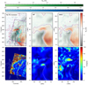 |
Fig. 8. Comparison of the non-LTE-inferred photospheric and chromospheric magnetic field (left column) with those from the magnetofrictional model (middle column) and the MHD model (right column). Top row: photospheric LOS magnetic field with azimuth arrows for the photospheric field (blue) and chromospheric field (green), colour-scaled according to the corresponding colour bars. We encourage using a PDF viewer to appreciate the photosphere-to-chromosphere changes in magnetic field azimuth. The inferred magnetic field has been taken at log τ500 = −1.1 (from non-LTE Fe I) and log τ500 = [ − 2.9, −4.1] (from Ca II 8542 Å) and the magnetic field map in the top left panel is identical to Fig. 5e, only including now also arrows for the chromospheric field azimuth (green). Bottom row: angle θ between the photospheric and chromospheric field vector of the inversions and models. The dashed lines (purple in the top row, white in the bottom row) indicate the photospheric LOS polarity inversion lines, while the cyan contours in the top left panel outline the Ca II flare ribbons. |
The top middle and right-hand panels (i.e. models) are relatively similar between each other, yet differ considerably in several aspects from the left-hand panel (i.e. inferred field). The overall distribution of positive and negative LOS polarities is similar between all three panels, but where the non-LTE inference of the magnetic field yields absolute LOS field strengths in excess of 4 kG in both photosphere and chromosphere in certain places, the simulations do not reach beyond 2.4 kG in the photosphere and 1.3 kG in the chromosphere anywhere. Similarly for the horizontal field, the inferred values of up to 5 kG in the photosphere and 4.6 kG in the chromosphere are two to three times larger than the maxima in the simulations. This is likely a combined effect of the pixel size difference between HMI and Hinode data, as well as the fact that the Hinode data sample two spectral lines with different Landé factors at high spectral resolution, leading to a weaker field from the HMI data and, consequently, lower values in the models that are based on that.
While more than half an hour apart, the two modelling results generally exhibit the same LOS field distribution reaching also similar strengths (both between about ±2 kG in the photosphere and ±1.3 kG in the chromosphere, though slightly stronger in the MF model). The MF model also has more extended strong-field concentrations than the MHD model. Even larger differences are found in the horizontal field strengths and especially in the azimuth pattern. Discrepancies in the latter are evident close to the polarity inversion line, where the field in the MF model (middle panel) is oriented at a larger angle to the polarity inversion line, while that of the MHD model (right panel) follows the inverse-S shape more closely. Also, the apparent source point of diverging positive field in the MF model (at (x, y) = (−12 Mm, 0 Mm) in the middle panel) lies some 6−7 Mm towards the north-west (i.e. upper right) in the MHD model (at (x, y) = (100 Mm, 74 Mm) in the right panel), while the “whirlpool-like” convergence to negative LOS field in the head of the inverse-S is similar in both, albeit stronger in the MHD results.
In strong LOS field regions, the photospheric and chromospheric azimuths are similar between the non-LTE inference and the models, whereas in weaker field areas the inferred azimuth appears more random. For all three panels, the photospheric and chromospheric azimuths are often similar, but the inferred azimuths show typically the largest angles between the photosphere and chromosphere – in particular in and close to the strong-field regions in the vicinity of the inverse-S shaped polarity inversion line. Overall, and considering the strong-field part of the FOV in particular, the inferred azimuths are best approached by those from the MHD model.
5.2. Photosphere-to-chromosphere field vector variation
The smoothness in change of the field vector orientation from the photosphere to the chromosphere in the models compared to the inversions is further emphasised in the bottom row of Fig. 8, showing maps of the angle θ(Bphot, Bchro) between the 3D photospheric and chromospheric magnetic field vectors. For most of the strong-field regions of the FOV the angle between the inferred field vectors is relatively small (below 50°), while strong deviations are found outside the sunspot penumbra (above the upper polarity inversion line, marked by the dashed white line). Here, the total field strength in both photosphere and chromosphere is small and the azimuth consequently difficult to disambiguate, resulting in θ displaying a confetti-coloured randomness. In the models, most of the FOV has relatively shallow angles between the photospheric and chromospheric field. Apart from the resolution and timing difference, both models tend to have the enhancements in θ in similar places, although at often larger magnitudes in the MHD model (e.g. the large patch of θ ≃ 50−100° around (x, y) = (94 Mm, 104 Mm)) and sometimes lacking a clear counterpart in the MF model (e.g. the band of θ ≃ 40−50° around (x, y) = (80 Mm, 75 Mm)). What stands out in all three panels is the arched head of the inverse-S shape, which shows angle differences between photosphere and chromosphere of at least about 50−65° in the models and of 50−140° from the observations. In the inferred field, these enhanced angle differences are found along most of the spine of the inverse-S (right of the dashed white line), where the MF model exhibits only a haze of 20−30° and the MHD model shows only a few localised enhancements of 30−50°. Also, while the observations have the entire inverse-S head light up in enhanced angles, the MF model is enhanced mostly in the eastern half (i.e. towards the left), while the MHD model has enhancements both at about (x, y) = (88 Mm, 92 Mm) and (x, y) = (97 Mm, 93 Mm), with smaller angles in between.
6. Discussion
6.1. Magnetic field approximations
Both the Milne-Eddington and spatially regularised weak-field approximation offer a computationally inexpensive way of obtaining the magnetic field vector from observations, compared to full-blown non-LTE inversions. At the same time, they come with limitations, as we also see in this study. In particular the Fe I Milne-Eddington inversion suffers from issues in locations where the Fe I lines are in emission, recovering the wrong sign for the LOS polarity (cf. Fig. 2) due to the linear source function assumed in the model. Unsurprisingly, these locations correspond well with those areas where white light flare emission in the HMI pseudocontinuum (obtained in the vicinity of Fe I 6173 Å) has been reported in previous studies (e.g. Fig. 5 in Romano et al. 2019 or Fig. 2 in Verma 2018). Furthermore, comparison with (non-)LTE inversions reveals that the default 5 kG saturation limit imposed on the MERLIN Milne-Eddington LOS and horizontal field may be too stringent here, a limitation previously noted also in non-flaring sunspots (e.g. Okamoto & Sakurai 2018), and this could play a general role in flares that occur in similarly complex configurations.
On the other hand, and despite the relatively coarse sampling of the Ca II 8542 Å line, the spatially regularised weak-field approximation does a good job at recovering a magnetic field vector that is very similar to that obtained from non-LTE inversions (cf. Fig. 6). Over 90% of the pixels have the non-LTE and WFA inclinations within 15° and their 3D field vectors within 25° of each other. The LOS component in particular is close to the non-LTE-inferred value in strong-field areas, while the transverse field exhibits a much larger scatter. This gets worse outside the sunspot, where the LOS field is weak and the field vector more horizontal, complicating retrieval of the transverse component (as Centeno 2018 already points out), even though the spatial constraint strongly mitigates the adverse effects of noise (Morosin et al. 2020). More than half of the strong-field pixels have a stronger horizontal and total field strength in the non-LTE inversions, while slightly less than half do so for the LOS field.
6.2. Weighing the need for non-LTE inversions of Fe I
Several studies over the past 50 years have investigated the effects of assuming LTE versus non-LTE in the formation of the Fe I lines (e.g. Athay & Lites 1972; Lites 1973; Rutten & Kostik 1982; Rutten 1988; Shchukina & Trujillo Bueno 2001; Holzreuter & Solanki 2012, 2013, 2015). Of particular interest for the present study are the effects on magnetic field strength and inclination that are reported by Smitha et al. (2020) when inverting in LTE either LTE or non-LTE synthesised Fe I profiles. Hence, a natural course has been to explore such effects for the data that we analysed.
In a qualitative sense, the differences in the inferred magnetic field components are minor when considering our LTE and non-LTE Fe I inversion results (cf. Fig. 2). Although there are obvious per-pixel differences, a similar map of positive and negative LOS polarities is found for both and the locations of stronger horizontal field coincide well between the two inversion approaches. The latter is supported quantitatively by the typically tighter correlation between LTE and non-LTE results for horizontal field strengths above ∼4.5 kG compared to those below (Fig. 3, second row). The largest differences are found in the inferred temperatures (Fig. 3, last row) and field azimuth, with typically higher temperatures by 500−1500 K in the non-LTE results and a spatially smoother counter-clockwise azimuth pattern in the negative Blos polarity (i.e. the “head” of the inverse-S) compared to the LTE inversions. One reason for this could be that the temperature increase required to fit the Fe I emission lines is larger in non-LTE than in LTE (and if the placement of such a temperature gradient is limited by the node description), this could lead to a discrepancy in the magnetic field as a result of a difference in the shape of the source function.
Nonetheless, as far as the magnetic field is concerned, there is no strong indication that would favour non-LTE over LTE inversions of Fe I, while for temperatures the differences can be significant, in particular at optical depths log τ500 = −1 and higher up in the atmosphere. Whether this is worth an increase of about a factor of two in computational cost to perform non-LTE inversions will, thus, depend on the particular scientific objective.
6.3. Photospheric and chromospheric magnetic field
Field strengths. In certain parts of the field of view, the (non-) LTE inversions with STiC yield a stronger field than the Milne-Eddington inversion and weak-field approximation, with values that are on the high end of (and for the chromospheric field much larger than) what has generally been reported, even for sunspots. For instance, the survey study by Livingston et al. (2006), analysing nearly 90 years worth of sunspot observations, highlights this in finding that a mere 0.2% of the sunspot group sample containing sunspots with photospheric field strengths in excess of 4 kG, only one case of which at 6.1 kG. At the same time, several recent studies have reported strong fields in sunspots. Okamoto & Sakurai (2018), using a Milne-Eddington inversion, find field strengths of over 5−6 kG between two opposite-polarity umbrae, with the 6302.5 Å Stokes I profile exhibiting clear Zeeman splitting. Field strengths of over 7 kG have been inferred by van Noort et al. (2013) and Siu-Tapia et al. (2019) from Fe I 6302 Å observations of sunspot penumbrae at locations that are associated with strong downflows and where the consequent evacuation may explain the large field strengths as probing sub-log τ500 = 0 heights. Castellanos Durán et al. (2020), employing a similar inversion approach on a sunspot lightbridge, find the field in excess of 5 kG at all inversion nodes and even up to 8.25 kG at log τ500 = 0.
In flares, most photospheric field strengths have typically been derived from SDO/HMI data. For instance, Sun et al. (2012) and Wang et al. (2012) investigated the same X2.2 flare and reported Bhor and Blos with values of 1.5 kG to over 2 kG, while Sadykov et al. (2016) studied an M1.0 flare with underlying absolute LOS field strengths of up to 3 kG. A C4.1 flare analysed by Guglielmino et al. (2016) occurred in a δ-spot with a LOS field up to about 1.5−2.0 kG, derived from both HMI and SST/CRISP Fe I 6301.5 Å data. Similar values have been reported from ground-based observations, for example, on the basis of LTE inversions of Si I 10827 Å, Kuckein et al. (2015) found total field strengths of order 1−2 kG in an M3.2 flare, while Gömöry et al. (2017) performed LTE inversion of Fe I 10783 Å and Si I 10786 Å, yielding Blos and Bhor of the order of 1.0−1.5 kG during an M1.8 flare in a δ-spot configuration. Liu et al. (2018b) reported Bhor of 0.2−1.0 kG and |Blos| of 1.5−2.5 kG in an M6.5 flare observed in Fe I 15648 Å. On the other hand, chromospheric field inferences in flares or filament eruptions are scarce and typically report values of a 0.3−2 kG and rarely more. For example, Sasso et al. (2014), with a few hundred Gauss in a activated filament during a flare observed in He I 10830 Å, Kleint (2017) and Kuridze et al. (2018), with ∼1.5 kG from Ca II 8542 Å observations of an X1 and M1.9 flare, respectively, as well as Libbrecht et al. (2019), with ∼2.5 kG from He I D3 observations of a C3.6 flare, or Kuckein et al. (2020), with up to 60 G LOS and up to 250 G horizontal field from He I 10830 Å observations of an erupting filament.
For the particular active region under scrutiny, Jurčák et al. (2018) report field strengths of order 2.5 kG from LTE inversions both during and after the X9.3 flare that followed the X2.2 flare, while Wang et al. (2018b) find transverse photospheric field of over 5.5 kG at the PIL from direct measurement of the Zeeman splitting in Fe I 15648 Å GST spectra, a few hours after the X9.3 flare. In addition, Anfinogentov et al. (2019) report exceptionally strong, kilogauss-order coronal magnetic fields about 5.5 h prior to the X2.2 flare based on a NLFFF reconstruction that is able to reproduce the gyroresonant emission observed with the Nobeyama Radio Heliograph. What is noteworthy is the fact that their results support the ∼5.5 kG field strengths reported by Wang et al. (2018b) and indicate field strengths of order 3.5−3.0 kG at 1−3 Mm heights. In this context it is, perhaps, not surprising that we find places where the horizontal and LOS field strengths reach an order of 5−6 kG in the photosphere and 3−4 kG in the chromosphere.
Given the exceptionally strong field that our inversions recovered, we also opted to consider a potential degeneracy between field strength and micro-turbulence. Fitting a turbulence-broadened profile might cause the inversion code to settle on a high magnetic field with low micro-turbulence, while observations in the ultraviolet have been found consistent with the presence of micro-turbulence in the chromosphere during (the onset of) flares at sites of both chromospheric evaporation and condensation (e.g. Milligan 2011; Harra et al. 2013; Jeffrey et al. 2018; Graham et al. 2020). However, where these strongest field values are inferred in the photosphere, the Zeeman splitting is often evident even in Stokes I (Fig. 4) and the individual components are narrow, arguing against non-resolved motions. Moreover, these pixels are largely found in coherent patches that are co-located with similarly coherent strong-field patches in the chromosphere (Figs. 5b and e) and we therefore trust the values inferred for both photosphere and chromosphere.
Height-dependent field vector. The non-LTE inversions of Fe I and Ca II provide photospheric and chromospheric field vectors and allow us, for the first time, to track from observations the orientation of the magnetic field vector with height in an X-class flare. In particular, the chromospheric field azimuth (derived from Stokes Q and U, which, in turn, are often plagued by noise in the chromosphere) is notoriously challenging to obtain even in flares and, consequently, few have made the attempt (Libbrecht et al. 2019). In the case of AR 12673, we benefit from the strong signal in these Stokes components as a result of the underlying sunspot, which enables us to confidently infer and disambiguate the chromospheric azimuth (Fig. 5).
The angle between the 3D photospheric and chromospheric field vectors is small for most of the strong-field part of the FOV, while there is an evident enhancement of some 40°–140° tracing the inverse-S polarity inversion line and coinciding remarkably well with the flare ribbon emission in Ca II 8542 Å (Fig. 8, left column panels). While the magnetic flux rope system that has been proposed in various studies (e.g. Liu et al. 2018a; Inoue et al. 2018; Romano et al. 2019; Price et al. 2019; Bamba et al. 2020) cannot be identified entirely in the inferred maps, it is nevertheless worth noting that the two patches of enhanced θ in the lower right panel of Fig. 8 appear to coincide with the footpoints of flux ropes FR1 and FR4 in Inoue et al. (2018). In addition, the concentrations of strong photospheric and chromospheric field (Figs. 5b and e) seem to be located at, or in the vicinity of, the flux rope footpoints F1 and F2 in Bamba et al. (2020). We therefore speculate that the observed angle enhancements in the inverse-S head (lower left panel) and the strong-field concentrations in the head and lower down along the spine may similarly be sampling flux rope footpoints and that our inferred chromospheric field is thus able to pick up at least part of the flux rope system.
6.4. Discrepancies with the numerical models
The most striking difference between the numerical models and inversions is in the amplitudes of both the LOS and transverse magnetic field. This can be partly attributed to the difference in spatial and spectral resolution of the HMI and Hinode SOT/SP instruments, but the pre-processing for both simulations plays an equally important role–if not more so. The latter is also evident when comparing the original HMI field vector with the field from both numerical models at z = 0 Mm. Inoue et al. (2018) use the pre-processing procedure by Wiegelmann et al. (2006), which modifies the observed magnetic field vector to fit the assumption of a force-free field. As a result, the transverse field can get significantly reduced, in this case by up to a factor of two in some places. For the magnetofrictional model, Price et al. (2019) apply spatial and temporal smoothing to ensure numerical stability of the simulations. In addition, the vector magnetic field maps are rebinned spatially in both approaches, by a factor of two and of four in the MHD and MF model, respectively. Combined, these effects result in a factor of two to three in field strength amplitude difference between the models and the inversions. We note here that we did not take the instrumental point spread function into account and that use of spatially coupled inversions (van Noort 2012; Asensio Ramos & de la Cruz Rodríguez 2015) would further increase the difference.
Obtaining the magnetic field vector accurately is extremely important in space weather modelling and prediction. Underestimating the field strength at the source has a direct impact on the estimate for the flux carried by a pre-eruptive flux rope and would result in a wrong estimate of its location and diameter, which, in turn, would produce a mismatch between the models and the field measured at Earth (Török et al. 2018). It is a well-recognised problem that an underestimate of the magnetic flux in observationally retrieved maps can lead to an underestimation of the interplanetary magnetic flux (Linker et al. 2017). This is especially true for the quiet Sun, where most of the flux remains invisible to current instruments (Danilovic et al. 2016). However, our results indicate that this may even be the case in active regions, despite the fact that the field there is strong and fills the whole surface area that is covered by a pixel.
The second noticeable difference between the models and inversions is the strong enhancement of some 40°–140° in the angle between the 3D photospheric and chromospheric field along the inverse-S polarity inversion line. This band is conspicuously absent in the MHD model snapshot of Inoue et al. (2018), corresponding to approximately 10 min before our inversions (Fig. 8, right column panels). Again, pre-processing may be the culprit behind this discrepancy, but it is conceivable that the increase in photosphere-to-chromosphere shear may be due to the field reconfiguration during the flare. The latter assumption fits in with the tether-cutting reconnection scenario proposed by Zou et al. (2019) in their two-step reconnection process, given that the soft X-ray flux lightcurve goes through a steep increase between 09:08 and 09:10 UT, which is where our Ca II snapshot lies dead in the middle of. On the other hand, in their NLFFF extrapolation, the reconnection that precedes and triggers the tether-cutting reconnection occurs in a null point outside the magnetic flux rope system, which unfortunately falls also outside our SST FOV. The increase in retrieved photosphere-to-chromosphere shear is also in agreement with the post-flare configuration proposed by Bamba et al. (2020).
Finally, an examination of the original HMI maps indicates that the position of the diverging positive polarity of the inverse-S does not significantly change in the time span of 09:12−09:24 UT. This suggests that the mismatch in footpoint location between observations and the MF model is likely due to the spatial smearing applied to the original field maps as part of the pre-processing for the latter.
7. Conclusions
In this paper, we present a comparison of the inferred photospheric and chromospheric magnetic fields during the confined X2.2 flare in NOAA AR 12673 on 6 September 2017 that has allowed, for the first time, a tracking of the variation in magnetic field vector orientation from the photosphere to the chromosphere in an X-class flare. Our results suggest that in the flare LTE formation of Fe I is not a faulty assumption per se, but, rather, that non-LTE inversions may yield a stronger LOS field in the lower layers (with median differences of up to 7−9%, depending on whether the full field or only flaring pixels are considered) and higher temperatures throughout (up to 25% for flaring pixels at log τ500 = −2.1). Also, the disambiguated non-LTE field azimuth presents a smoother map in the strongest field areas than the LTE results. Without knowledge of the true solution, however, we cannot rule in favour of one over the other. Thus, performing a similar investigation of a flare simulation would be worthwhile.
On the other hand, we see that for this case, Milne-Eddington inversions are an oversimplification that suffer in the presence of Fe I emission profiles, resulting in erroneous LOS polarities. Allowing for depth-dependence is ultimately necessary for a proper inference of the magnetic field vector in this (and likely most) flaring region(s). In the chromosphere, the spatially-constrained weak-field approximation offers an excellent estimate of the non-LTE-inferred magnetic field vector, where the field strengths may be underestimated by a only few percent compared to actual inversions.
While the chromospheric field points approximately in the same direction as the photospheric field over most of the umbrae, there is a marked band of enhanced angles (40°–140°) in the 3D photosphere-to-chromosphere field vector that closely traces the inverse-S polarity inversion line. It coincides almost entirely with the location of the flare ribbons observed in Ca II 8542 Å and, thus, we assume it is likely due to the flare-induced field reconfiguration.
During the flare, there are coherent patches of strong LOS and horizontal field that persist from the photosphere (at > 4.5 kG) to the chromosphere (at > 3 kG) and we find some pixels with either field component in excess of even 5 kG in both photospheric and chromospheric field maps. Both these strong-field concentrations and the enhanced photosphere-to-chromosphere shear in the inverse-S head are found in close proximity to flux rope footpoints proposed from modelling and our inversions thus confirm such a flux rope system configuration. However, compared to the models, the amplitudes of the inferred field strengths are larger by up to a factor of two to three, while the photosphere-to-chromosphere shear is also stronger, more concentrated, and more finely structured. The pre-processing and lower spatial resolution of the numerical models are both likely to be the culprits behind these discrepancies.
Hence, while full-blown (non-)LTE inversions remain necessary to obtain a depth-stratified atmospheric model, the spatially regularised WFA represents a powerful tool for quickly obtaining the chromospheric magnetic field vector over a large field of view. In turn, this can be used as an additional boundary constraint in the (flaring) active region numerical modelling or can otherwise help in improving existing models. Validating or assessing these models remains very difficult, as they are usually limited to photospheric observations and the coronal EUV emission, which the (non-thermodynamic) models do not directly provide. Additional constraints in the form of chromospheric field maps are, therefore, valuable.
The discrepancies in field strength and smoothness between the models and inversions further emphasise the need for higher spatial resolution in the models to better constrain pre-eruptive flux ropes since underestimating the magnetic flux therein will impact the accuracy of CME evolution modelling for space weather predictions.
Acknowledgments
GV is supported by a grant from the Swedish Civil Contingencies Agency (MSB). SD acknowledges the Vinnova support through the grant MSCA 796805. This research has received funding from the European Union’s Horizon 2020 research and innovation programme under grant agreement No 824135. JL is supported by a grant from the Knut and Alice Wallenberg foundation (2016.0019). JdlCR is supported by grants from the Swedish Research Council (2015-03994), the Swedish National Space Board (128/15) and the Swedish Civil Contingencies Agency (MSB). This project has received funding from the European Research Council (ERC) under the European Union’s Horizon 2020 research and innovation programme (SUNMAG, grant agreement 759548). AR acknowledges support from STFC under grant No. ST/P000304/1. This project has received funding from the European Research Council (ERC) under the European Union’s Horizon 2020 research and innovation programme (SolMAG, grant agreement No 724391). This project has received funding from the Academy of Finland (FORESAIL, grant number 312390; SMASH, grant number 310445). We are grateful to H. N. Smitha at the Max-Planck-Institut für Sonnensystemforschung for providing the Fe I model atom that we used in our inversions and to Emilia Kilpua for useful comments. The Institute for Solar Physics is supported by a grant for research infrastructures of national importance from the Swedish Research Council (registration number 2017-00625). The Swedish 1 m Solar Telescope is operated on the island of La Palma by the Institute for Solar Physics of Stockholm University in the Spanish Observatorio del Roque de los Muchachos of the Instituto de Astrofísica de Canarias. Hinode is a Japanese mission developed and launched by ISAS/JAXA, with NAOJ as domestic partner and NASA and STFC (UK) as international partners. It is operated by these agencies in co-operation with ESA and NSC (Norway). The SDO/HMI data used are courtesy of NASA/SDO and HMI science team. The inversions were performed on resources provided by the Swedish National Infrastructure for Computing (SNIC) at the National Supercomputer Centre at Linköping University. We thank R. Shine as Hinode SOT CO for scheduling the SOT/SP observations used here. We made much use of NASA’s Astrophysics Data System Bibliographic Services. Last but not least, we acknowledge the community effort to develop open-source packages used in this work: numpy (Oliphant 2006; numpy.org), matplotlib (Hunter 2007; matplotlib.org), scipy (Virtanen et al. 2020; scipy.org), astropy (Astropy Collaboration 2013, 2018; astropy.org), sunpy (The SunPy Community 2020; sunpy.org).
References
- Anfinogentov, S. A., Stupishin, A. G., Mysh’yakov, I. I., & Fleishman, G. D. 2019, ApJ, 880, L29 [CrossRef] [Google Scholar]
- Asensio Ramos, A., & de la Cruz Rodríguez, J. 2015, A&A, 577, A140 [NASA ADS] [CrossRef] [EDP Sciences] [Google Scholar]
- Astropy Collaboration (Robitaille, T. P., et al.) 2013, A&A, 558, A33 [NASA ADS] [CrossRef] [EDP Sciences] [Google Scholar]
- Astropy Collaboration (Price-Whelan, A. M., et al.) 2018, AJ, 156, 123 [Google Scholar]
- Athay, R. G., & Lites, B. W. 1972, ApJ, 176, 809 [NASA ADS] [CrossRef] [Google Scholar]
- Bamba, Y., Inoue, S., & Imada, S. 2020, ApJ, 894, 29 [CrossRef] [Google Scholar]
- Bjørgen, J. P., Leenaarts, J., Rempel, M., et al. 2019, A&A, 631, A33 [NASA ADS] [CrossRef] [EDP Sciences] [Google Scholar]
- Bobra, M. G., & Couvidat, S. 2015, ApJ, 798, 135 [NASA ADS] [CrossRef] [Google Scholar]
- Bobra, M. G., Sun, X., Hoeksema, J. T., et al. 2014, Sol. Phys., 289, 3549 [NASA ADS] [CrossRef] [Google Scholar]
- Castellanos Durán, J. S., Lagg, A., Solanki, S. K., & van Noort, M. 2020, ApJ, 895, 129 [CrossRef] [Google Scholar]
- Centeno, R. 2018, ApJ, 866, 89 [NASA ADS] [CrossRef] [Google Scholar]
- Danilovic, S., Rempel, M., van Noort, M., & Cameron, R. 2016, A&A, 594, A103 [NASA ADS] [CrossRef] [EDP Sciences] [Google Scholar]
- de la Cruz Rodríguez, J. 2019, A&A, 631, A153 [NASA ADS] [CrossRef] [EDP Sciences] [Google Scholar]
- de la Cruz Rodríguez, J., & Piskunov, N. 2013, ApJ, 764, 33 [NASA ADS] [CrossRef] [Google Scholar]
- de la Cruz Rodríguez, J., Rouppe van der Voort, L., Socas-Navarro, H., & van Noort, M. 2013, A&A, 556, A115 [NASA ADS] [CrossRef] [EDP Sciences] [Google Scholar]
- de la Cruz Rodríguez, J., Löfdahl, M. G., Sütterlin, P., Hillberg, T., & Rouppe van der Voort, L. 2015, A&A, 573, A40 [NASA ADS] [CrossRef] [EDP Sciences] [Google Scholar]
- de la Cruz Rodríguez, J., Leenaarts, J., & Asensio Ramos, A. 2016, ApJ, 830, L30 [NASA ADS] [CrossRef] [Google Scholar]
- de la Cruz Rodríguez, J., Leenaarts, J., Danilovic, S., & Uitenbroek, H. 2019, A&A, 623, A74 [NASA ADS] [CrossRef] [EDP Sciences] [Google Scholar]
- De Rosa, M. L., Schrijver, C. J., Barnes, G., et al. 2009, ApJ, 696, 1780 [Google Scholar]
- Díaz Baso, C. J., de la Cruz Rodríguez, J., & Danilovic, S. 2019, A&A, 629, A99 [CrossRef] [EDP Sciences] [Google Scholar]
- Fleishman, G., Mysh’yakov, I., Stupishin, A., Loukitcheva, M., & Anfinogentov, S. 2019, ApJ, 870, 101 [CrossRef] [Google Scholar]
- Florios, K., Kontogiannis, I., Park, S.-H., et al. 2018, Sol. Phys., 293, 28 [CrossRef] [Google Scholar]
- Georgoulis, M. K., & Rust, D. M. 2007, ApJ, 661, L109 [NASA ADS] [CrossRef] [Google Scholar]
- Gömöry, P., Balthasar, H., Kuckein, C., et al. 2017, A&A, 602, A60 [NASA ADS] [CrossRef] [EDP Sciences] [Google Scholar]
- Graham, D. R., Cauzzi, G., Zangrilli, L., et al. 2020, ApJ, 895, 6 [CrossRef] [Google Scholar]
- Guglielmino, S. L., Zuccarello, F., Romano, P., et al. 2016, ApJ, 819, 157 [NASA ADS] [CrossRef] [Google Scholar]
- Harra, L. K., Matthews, S., Culhane, J. L., et al. 2013, ApJ, 774, 122 [NASA ADS] [CrossRef] [Google Scholar]
- Harvey, J. W. 2012, Sol. Phys., 280, 69 [CrossRef] [Google Scholar]
- Henriques, V. M. J. 2012, A&A, 548, A114 [NASA ADS] [CrossRef] [EDP Sciences] [Google Scholar]
- Holzreuter, R., & Solanki, S. K. 2012, A&A, 547, A46 [NASA ADS] [CrossRef] [EDP Sciences] [Google Scholar]
- Holzreuter, R., & Solanki, S. K. 2013, A&A, 558, A20 [NASA ADS] [CrossRef] [EDP Sciences] [Google Scholar]
- Holzreuter, R., & Solanki, S. K. 2015, A&A, 582, A101 [NASA ADS] [CrossRef] [EDP Sciences] [Google Scholar]
- Hou, Y. J., Zhang, J., Li, T., Yang, S. H., & Li, X. H. 2018, A&A, 619, A100 [NASA ADS] [CrossRef] [EDP Sciences] [Google Scholar]
- Hunter, J. D. 2007, Comput. Sci. Eng., 9, 90 [NASA ADS] [CrossRef] [Google Scholar]
- Inoue, S., Shiota, D., Bamba, Y., & Park, S.-H. 2018, ApJ, 867, 83 [NASA ADS] [CrossRef] [Google Scholar]
- Jeffrey, N. L. S., Fletcher, L., Labrosse, N., & Simões, P. J. A. 2018, Sci. Adv., 4, 2794 [CrossRef] [Google Scholar]
- Jiang, C., Zou, P., Feng, X., et al. 2018, ApJ, 869, 13 [NASA ADS] [CrossRef] [Google Scholar]
- Jonas, E., Bobra, M., Shankar, V., Todd Hoeksema, J., & Recht, B. 2018, Sol. Phys., 293, 48 [CrossRef] [Google Scholar]
- Judge, P. G., Kleint, L., & Sainz Dalda, A. 2015, ApJ, 814, 100 [NASA ADS] [CrossRef] [Google Scholar]
- Jurčák, J., Kašparová, J., Švanda, M., & Kleint, L. 2018, A&A, 620, A183 [CrossRef] [EDP Sciences] [Google Scholar]
- Kilpua, E. K. J., Lugaz, N., Mays, M. L., & Temmer, M. 2019, Space Weather, 17, 498 [NASA ADS] [CrossRef] [Google Scholar]
- Kleint, L. 2017, ApJ, 834, 26 [NASA ADS] [CrossRef] [Google Scholar]
- Kosugi, T., Matsuzaki, K., Sakao, T., et al. 2007, Sol. Phys., 243, 3 [Google Scholar]
- Kuckein, C., Collados, M., & Manso Sainz, R. 2015, ApJ, 799, L25 [NASA ADS] [CrossRef] [Google Scholar]
- Kuckein, C., González Manrique, S. J., Kleint, L., & Asensio Ramos, A. 2020, A&A, 640, A71 [CrossRef] [EDP Sciences] [Google Scholar]
- Kuridze, D., Henriques, V. M. J., Mathioudakis, M., et al. 2018, ApJ, 860, 10 [NASA ADS] [CrossRef] [Google Scholar]
- Kuridze, D., Mathioudakis, M., Morgan, H., et al. 2019, ApJ, 874, 126 [NASA ADS] [CrossRef] [Google Scholar]
- Kusano, K., Bamba, Y., Yamamoto, T. T., et al. 2012, ApJ, 760, 31 [NASA ADS] [CrossRef] [Google Scholar]
- Landi Degl’Innocenti, E. 1992, in Magnetic Field Measurements, eds. F. Sánchez, M. Collados, & M. Vázquez, 71 [Google Scholar]
- Landi Degl’Innocenti, E., & Landolfi, M. 2004, Polarization in Spectral Lines (Dordrecht: Kluwer Academic Publishers), 307 [Google Scholar]
- Leka, K. D., & Barnes, G. 2003, ApJ, 595, 1296 [CrossRef] [Google Scholar]
- Leka, K. D., & Barnes, G. 2007, ApJ, 656, 1173 [NASA ADS] [CrossRef] [Google Scholar]
- Leka, K. D., Barnes, G., & Crouch, A. 2014, Astrophysics Source Code Library [record ascl:1404.007] [Google Scholar]
- Libbrecht, T., de la Cruz Rodríguez, J., Danilovic, S., Leenaarts, J., & Pazira, H. 2019, A&A, 621, A35 [NASA ADS] [CrossRef] [EDP Sciences] [Google Scholar]
- Linker, J. A., Caplan, R. M., Downs, C., et al. 2017, ApJ, 848, 70 [NASA ADS] [CrossRef] [Google Scholar]
- Lites, B. W. 1973, Sol. Phys., 32, 283 [NASA ADS] [CrossRef] [Google Scholar]
- Liu, L., Cheng, X., Wang, Y., et al. 2018a, ApJ, 867, L5 [NASA ADS] [CrossRef] [Google Scholar]
- Liu, C., Cao, W., Chae, J., et al. 2018b, ApJ, 869, 21 [CrossRef] [Google Scholar]
- Livingston, W., Harvey, J. W., Malanushenko, O. V., & Webster, L. 2006, Sol. Phys., 239, 41 [Google Scholar]
- Löfdahl, M. G., Hillberg, T., de la Cruz Rodriguéz, J., et al. 2018, ArXiv e-prints [arXiv:1804.03030] [Google Scholar]
- Lumme, E., Pomoell, J., & Kilpua, E. K. J. 2017, Sol. Phys., 292, 191 [NASA ADS] [CrossRef] [Google Scholar]
- McCloskey, A. E., Gallagher, P. T., & Bloomfield, D. S. 2016, Sol. Phys., 291, 1711 [CrossRef] [Google Scholar]
- Metcalf, T. R. 1994, Sol. Phys., 155, 235 [Google Scholar]
- Metcalf, T. R., Leka, K. D., Barnes, G., et al. 2006, Sol. Phys., 237, 267 [Google Scholar]
- Milligan, R. O. 2011, ApJ, 740, 70 [NASA ADS] [CrossRef] [Google Scholar]
- Morosin, R., de la Cruz Rodriguez, J., Vissers, G. J. M., & Yadav, R. 2020, A&A, 642, A210 [CrossRef] [EDP Sciences] [Google Scholar]
- Nishizuka, N., Sugiura, K., Kubo, Y., Den, M., & Ishii, M. 2018, ApJ, 858, 113 [NASA ADS] [CrossRef] [Google Scholar]
- Okamoto, T. J., & Sakurai, T. 2018, ApJ, 852, L16 [Google Scholar]
- Oliphant, T. E. 2006, A Guide to NumPy (USA: Trelgol Publishing), 1 [Google Scholar]
- Panos, B., & Kleint, L. 2020, ApJ, 891, 17 [CrossRef] [Google Scholar]
- Pariat, E., Leake, J. E., Valori, G., et al. 2017, A&A, 601, A125 [NASA ADS] [CrossRef] [EDP Sciences] [Google Scholar]
- Pesnell, W. D., Thompson, B. J., & Chamberlin, P. C. 2012, Sol. Phys., 275, 3 [Google Scholar]
- Pietarila, A., Socas-Navarro, H., & Bogdan, T. 2007, ApJ, 663, 1386 [Google Scholar]
- Pietrow, A. G. M., Kiselman, D., de la Cruz Rodríguez, J., et al. 2020, A&A, 644, A43 [CrossRef] [EDP Sciences] [Google Scholar]
- Piskunov, N., & Valenti, J. A. 2017, A&A, 597, A16 [NASA ADS] [CrossRef] [EDP Sciences] [Google Scholar]
- Pomoell, J., Lumme, E., & Kilpua, E. 2019, Sol. Phys., 294, 41 [NASA ADS] [CrossRef] [Google Scholar]
- Price, D. J., Pomoell, J., Lumme, E., & Kilpua, E. K. J. 2019, A&A, 628, A114 [CrossRef] [EDP Sciences] [Google Scholar]
- Quinn, S., Reid, A., Mathioudakis, M., et al. 2019, ApJ, 881, 82 [CrossRef] [Google Scholar]
- Romano, P., Elmhamdi, A., Falco, M., et al. 2018, ApJ, 852, L10 [CrossRef] [Google Scholar]
- Romano, P., Elmhamdi, A., & Kordi, A. S. 2019, Sol. Phys., 294, 4 [NASA ADS] [CrossRef] [Google Scholar]
- Rutten, R. J. 1988, Astrophys. Space Sci. Lib., 138, 185 [CrossRef] [Google Scholar]
- Rutten, R. J., & Kostik, R. I. 1982, A&A, 115, 104 [NASA ADS] [Google Scholar]
- Sadykov, V. M., Kosovichev, A. G., Sharykin, I. N., Zimovets, I. V., & Vargas Dominguez, S. 2016, ApJ, 828, 4 [CrossRef] [Google Scholar]
- Sasso, C., Lagg, A., & Solanki, S. K. 2014, A&A, 561, A98 [NASA ADS] [CrossRef] [EDP Sciences] [Google Scholar]
- Scharmer, G. B., Bjelksjo, K., Korhonen, T. K., Lindberg, B., & Petterson, B. 2003, SPIE Conf. Ser., 4853, 341 [Google Scholar]
- Scharmer, G. B., Narayan, G., Hillberg, T., et al. 2008, ApJ, 689, L69 [Google Scholar]
- Scherrer, P. H., Schou, J., Bush, R. I., et al. 2012, Sol. Phys., 275, 207 [Google Scholar]
- Schou, J., Scherrer, P. H., Bush, R. I., et al. 2012, Sol. Phys., 275, 229 [Google Scholar]
- Schrijver, C. J. 2007, ApJ, 655, L117 [Google Scholar]
- Shchukina, N., & Trujillo Bueno, J. 2001, ApJ, 550, 970 [NASA ADS] [CrossRef] [Google Scholar]
- Shine, R. A., Title, A. M., Tarbell, T. D., et al. 1994, ApJ, 430, 413 [NASA ADS] [CrossRef] [Google Scholar]
- Siu-Tapia, A., Lagg, A., van Noort, M., Rempel, M., & Solanki, S. K. 2019, A&A, 631, A99 [CrossRef] [EDP Sciences] [Google Scholar]
- Smitha, H. N., Holzreuter, R., van Noort, M., & Solanki, S. K. 2020, A&A, 633, A157 [NASA ADS] [CrossRef] [EDP Sciences] [Google Scholar]
- Sun, X., Hoeksema, J. T., Liu, Y., et al. 2012, ApJ, 748, 77 [NASA ADS] [CrossRef] [Google Scholar]
- The SunPy Community (Barnes, W. T., et al.) 2020, ApJ, 890, 68 [CrossRef] [Google Scholar]
- Toriumi, S., Takasao, S., Cheung, M. C. M., et al. 2020, ApJ, 890, 103 [CrossRef] [Google Scholar]
- Török, T., Downs, C., Linker, J. A., et al. 2018, ApJ, 856, 75 [Google Scholar]
- Tsuneta, S., Ichimoto, K., Katsukawa, Y., et al. 2008, Sol. Phys., 249, 167 [NASA ADS] [CrossRef] [Google Scholar]
- Uitenbroek, H. 2001, ApJ, 557, 389 [NASA ADS] [CrossRef] [Google Scholar]
- van Noort, M. 2012, A&A, 548, A5 [NASA ADS] [CrossRef] [EDP Sciences] [Google Scholar]
- van Noort, M., Rouppe van der Voort, L., & Löfdahl, M. G. 2005, Sol. Phys., 228, 191 [Google Scholar]
- van Noort, M., Lagg, A., Tiwari, S. K., & Solanki, S. K. 2013, A&A, 557, A24 [NASA ADS] [CrossRef] [EDP Sciences] [Google Scholar]
- Verma, M. 2018, A&A, 612, A101 [NASA ADS] [CrossRef] [EDP Sciences] [Google Scholar]
- Virtanen, P., Gommers, R., Oliphant, T. E., et al. 2020, Nat. Meth., 17, 261 [Google Scholar]
- Vissers, G., & Rouppe van der Voort, L. 2012, ApJ, 750, 22 [NASA ADS] [CrossRef] [Google Scholar]
- Wang, S., Liu, C., Liu, R., et al. 2012, ApJ, 745, L17 [NASA ADS] [CrossRef] [Google Scholar]
- Wang, R., Liu, Y. D., Hoeksema, J. T., Zimovets, I. V., & Liu, Y. 2018a, ApJ, 869, 90 [CrossRef] [Google Scholar]
- Wang, H., Yurchyshyn, V., Liu, C., et al. 2018b, Res. Notes Am. Astron. Soc., 2, 8 [CrossRef] [Google Scholar]
- Wiegelmann, T., Inhester, B., & Sakurai, T. 2006, Sol. Phys., 233, 215 [NASA ADS] [CrossRef] [Google Scholar]
- Yang, S., Zhang, J., Zhu, X., & Song, Q. 2017, ApJ, 849, L21 [NASA ADS] [CrossRef] [Google Scholar]
- Zou, P., Jiang, C., Feng, X., et al. 2019, ApJ, 870, 97 [NASA ADS] [CrossRef] [Google Scholar]
- Zuccarello, F. P., Pariat, E., Valori, G., & Linan, L. 2018, ApJ, 863, 41 [Google Scholar]
All Tables
All Figures
|
Fig. 1. Overview of the analysed data, showing the SDO/HMI-derived SHARP LOS magnetic field from Fe I 6173 Å (left), Hinode/SP continuum near Fe I 6302 Å (middle) and SST/CRISP Ca II 8542 Å red wing at +0.5 Å (right). The Hinode and SST fields of view are indicated in the first two panels with green and purple boxes, respectively, while the dashed light green box in the first two panels outlines the cut-out of Fig. 2. The cyan contours in the middle panel indicate locations where the Fe I lines are in emission. Times in UT are indicated in the top left of each panel (for Hinode SOT/SP the time corresponds to the middle of the slit raster-scan). The vertical stripes in the middle panel are due to missing data. |
| In the text | |
|
Fig. 2. Line of sight and transverse magnetic field from STiC (non-)LTE inversions of the Fe I Hinode data over the sub-field indicated by the dashed green box in Fig. 1. From left to right the columns show the photospheric field at different log τ500 depths as specified in the top left corner of each panel, both for LTE (top row) and non-LTE (bottom row) inversions. The maps are of the LOS field (scaled according to the right-hand colour bar), while the blue arrows indicate the azimuth direction, where their hue reflects the horizontal field strength (according to the top colour bar). All panels are colour-scaled between the same values with both LOS and horizontal field strengths clipped to the range wherein 98% of the pixels fall. Bright green contours indicate where the horizontal field is in excess of 5 kG, while the cyan contours in the first column highlight where the Fe I lines are in emission. The coloured plus signs mark the locations for which (non-)LTE profile fits are shown in Fig. 4. |
| In the text | |
|
Fig. 3. Two-dimensional histograms of non-LTE versus LTE LOS magnetic field strength (top row), horizontal field strength (middle row), and temperature (bottom row) for the flaring pixels (i.e. within cyan contours in Fig. 2) at three log τ500 depths. The Pearson correlation number is shown in the top left of each panel and the log τ500 depth within parenthesis in the top row panels (for magnetic field) and bottom row panels (for temperature), while the straight lines indicate what would be linear relationship. |
| In the text | |
|
Fig. 4. Fe I 6301.5 Å and 6302.5 Å profiles from observations and (non-)LTE inversions. Each column shows (from top to bottom) Stokes I, Q, U and V profiles as observed (coloured dots) and as fitted in LTE (grey dashed line) and in non-LTE (solid black line). The colour coding corresponds to the identically coloured plus markers in the left-hand panels of Fig. 2. The numbers above each column indicate the non-LTE-inferred Blos and Bhor at log τ500 = −0.5. |
| In the text | |
|
Fig. 5. Chromospheric and photospheric magnetic field from the inversion methods that we applied. Panel a: chromospheric LOS field maps with green azimuth arrows coloured according to its horizontal field strength from the spatially regularised WFA. Panel b: same as panel a but from STiC non-LTE inversions. The contours mark where the field exceeds 4.5 kG in the photosphere and 3 kG in the chromosphere for Blos (cyan) and the same thresholds for Bhor (light green). The coloured plus markers indicate the locations for which Fig. 7 shows Ca II 8542 Å profile fits. Panel c: angle difference θ(BWFA, BSTiC) between the WFA and non-LTE three-dimensional (3D) field vectors, clipped to 100°. The dashed white contours highlight the regions where the WFA field strength exceeds 2 kG (selected pixels for Fig. 6). Panel d: photospheric LOS field maps with blue azimuth arrows as derived in the Milne-Eddington inversion. The black box indicates the SST FOV, while the contours highlight where the Fe I lines are in emission. Panel e: same as panel d but from the non-LTE inversions and contours as in panel b. The colour bars in the lower right are for the LOS field (grey-white-red), horizontal field in the photosphere (blue) and chromosphere (green), and the angle θ (rainbow). The colour bar range for the magnetic field strengths is representative of 98% of the pixels (as in Fig. 2). |
| In the text | |
|
Fig. 6. 2D histograms of non-LTE versus WFA LOS magnetic field strength (left), horizontal field strength (middle) and histograms of angle differences (right) between the 3D field vector as recovered from the WFA and non-LTE STiC inversions (solid blue) and between their field inclinations γWFA and γSTiC (dashed red) for pixels where the total WFA magnetic field strength exceeds 2 kG (white contours in Fig. 5d). Format for the left two panels as in Fig. 3. |
| In the text | |
|
Fig. 7. Ca II 8542 Å profiles from observations and non-LTE inversions for the coloured plus markers in Fig. 5b. Format as for Fig. 4, except that only non-LTE fitted profiles are shown (solid grey). The numbers above each column indicate the inferred Blos and Bhor averaged over log τ500 = [ − 2.9, −4.1]. |
| In the text | |
|
Fig. 8. Comparison of the non-LTE-inferred photospheric and chromospheric magnetic field (left column) with those from the magnetofrictional model (middle column) and the MHD model (right column). Top row: photospheric LOS magnetic field with azimuth arrows for the photospheric field (blue) and chromospheric field (green), colour-scaled according to the corresponding colour bars. We encourage using a PDF viewer to appreciate the photosphere-to-chromosphere changes in magnetic field azimuth. The inferred magnetic field has been taken at log τ500 = −1.1 (from non-LTE Fe I) and log τ500 = [ − 2.9, −4.1] (from Ca II 8542 Å) and the magnetic field map in the top left panel is identical to Fig. 5e, only including now also arrows for the chromospheric field azimuth (green). Bottom row: angle θ between the photospheric and chromospheric field vector of the inversions and models. The dashed lines (purple in the top row, white in the bottom row) indicate the photospheric LOS polarity inversion lines, while the cyan contours in the top left panel outline the Ca II flare ribbons. |
| In the text | |
Current usage metrics show cumulative count of Article Views (full-text article views including HTML views, PDF and ePub downloads, according to the available data) and Abstracts Views on Vision4Press platform.
Data correspond to usage on the plateform after 2015. The current usage metrics is available 48-96 hours after online publication and is updated daily on week days.
Initial download of the metrics may take a while.