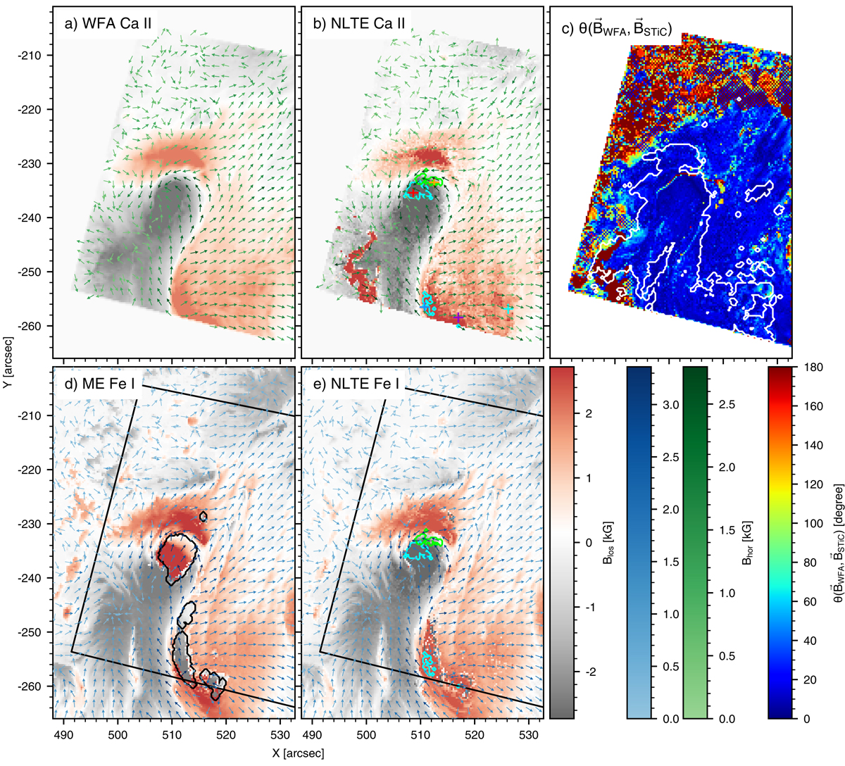
Chromospheric and photospheric magnetic field from the inversion methods that we applied. Panel a: chromospheric LOS field maps with green azimuth arrows coloured according to its horizontal field strength from the spatially regularised WFA. Panel b: same as panel a but from STiC non-LTE inversions. The contours mark where the field exceeds 4.5 kG in the photosphere and 3 kG in the chromosphere for B_los (cyan) and the same thresholds for B_hor (light green). The coloured plus markers indicate the locations for which Fig. 7 shows Ca II 8542 Å profile fits. Panel c: angle difference θ(B_WFA, B_STiC) between the WFA and non-LTE three-dimensional (3D) field vectors, clipped to 100°. The dashed white contours highlight the regions where the WFA field strength exceeds 2 kG (selected pixels for Fig. 6). Panel d: photospheric LOS field maps with blue azimuth arrows as derived in the Milne-Eddington inversion. The black box indicates the SST FOV, while the contours highlight where the Fe I lines are in emission. Panel e: same as panel d but from the non-LTE inversions and contours as in panel b. The colour bars in the lower right are for the LOS field (grey-white-red), horizontal field in the photosphere (blue) and chromosphere (green), and the angle θ (rainbow). The colour bar range for the magnetic field strengths is representative of 98% of the pixels (as in Fig. 2).