| Issue |
A&A
Volume 644, December 2020
|
|
|---|---|---|
| Article Number | A5 | |
| Number of page(s) | 10 | |
| Section | Interstellar and circumstellar matter | |
| DOI | https://doi.org/10.1051/0004-6361/202039282 | |
| Published online | 24 November 2020 | |
Compressed magnetized shells of atomic gas and the formation of the Corona Australis molecular cloud
1
Rudjer Bošković Institute,
Bijenička cesta 54,
10000
Zagreb,
Croatia
e-mail: This email address is being protected from spambots. You need JavaScript enabled to view it.
2
Jeremiah Horrocks Institute, University of Central Lancashire,
Preston,
Lancashire,
PR1 2HE, UK
3
Instituto de Astrofisica e Ciencias do Espaco, Universidade do Porto, CAUP, Rua das Estrelas,
4150-762
Porto, Portugal
4
Laboratoire d’Astrophysique (AIM), CEA/DRF, CNRS, Université Paris-Saclay, Université Paris Diderot, Sorbonne Paris Cité,
91191
Gif-sur-Yvette, France
5
Canadian Institute for Theoretical Astrophysics, University of Toronto,
Toronto,
ON
M5S 3H8, Canada
Received:
28
August
2020
Accepted:
20
October
2020
Abstract
We present the identification of the previously unnoticed physical association between the Corona Australis molecular cloud (CrA), traced by interstellar dust emission, and two shell-like structures observed with line emission of atomic hydrogen (HI) at 21 cm. Although the existence of the two shells had already been reported in the literature, the physical link between the HI emission and CrA had never been highlighted until now. We used both Planck and Herschel data to trace dust emission and the Galactic All Sky HI Survey (GASS) to trace HI. The physical association between CrA and the shells is assessed based both on spectroscopic observations of molecular and atomic gas and on dust extinction data with Gaia. The shells are located at a distance between ~140 and ~190 pc, which is comparable to the distance of CrA, which we derived as (150.5 ± 6.3) pc. We also employed dust polarization observations from Planck to trace the magnetic-field structure of the shells. Both of them show patterns of magnetic-field lines following the edge of the shells consistently with the magnetic-field morphology of CrA. We estimated the magnetic-field strength at the intersection of the two shells via the Davis-Chandrasekhar-Fermi (DCF) method. Despite the many caveats that are behind the DCF method, we find a magnetic-field strength of (27 ± 8) μG, which is at least a factor of two larger than the magnetic-field strength computed off of the HI shells. This value is also significantly larger compared to the typical values of a few μG found in the diffuse HI gas from Zeeman splitting. We interpret this as the result of magnetic-field compression caused by the shell expansion. This study supports a scenario of molecular-cloud formation triggered by supersonic compression of cold magnetized HI gas from expanding interstellar bubbles.
Key words: ISM: clouds / ISM: bubbles / ISM: magnetic fields / ISM: structure / evolution / ISM: kinematics and dynamics
Now working for McBraida Plc, Bristol, UK.
© ESO 2020
1 Introduction
Molecular clouds are the birth sites of stars in the Galaxy (e.g., Hennebelle & Falgarone 2012; Ballesteros-Paredes et al. 2020; Chevance et al. 2020). Their formation is a key step in understanding the efficiency of converting gas into stars in the interstellar medium (ISM), which represents a long-standing, yet unsolved, problem (Zuckerman & Evans 1974). The complex network of filaments, which structures matter in molecular clouds and plays a key role in the star formation process (i.e., André et al. 2014; Arzoumanian et al. 2019), is likely produced by the interaction between magneto-turbulent and gravitational instabilities (Hennebelle & Inutsuka 2019). However, large-scale magneto-hydrodynamic (MHD) flows are theoretically able to convert diffuse atomic gas into colder molecular gas only in the presence of multiple episodes of supersonic compression (Inutsuka et al. 2015). These multiple large-scale compressions are possibly set up by interacting bubbles and shells caused by feedback processes, such as stellar winds and supernova explosions (McClure-Griffiths et al. 2002) or high-velocity gas falling into the Galactic plane (Heitsch & Putman 2009).
Observations of external galaxies, such as the Large Magellanic cloud (Dawson et al. 2013), and of the Galactic plane (Dawson et al. 2015) have shown a strong association between molecular gas formation and superbubbles. Close-by molecular clouds in the Gould Belt – at a distance from the Sun of d < 500 pc – such as Orion (Soler et al. 2018; Joubaud et al. 2019; Könyves et al. 2020), Taurus, Perseus (Shimajiri et al. 2019), and Ophiuchus (Ladjelate et al. 2020), were also found to be shaped by large-scale compression from expanding shells and bubbles in their magnetized surroundings.
In this work we present the case of a rather isolated molecular cloud in the southern sky, the Corona Australis molecular cloud (CrA). We highlight the previously unnoticed association between two large-scale shells of atomic hydrogen (HI) with CrA as traced by interstellar dust and carbon monoxide (CO). We also discuss their common magnetic-field properties.
The paper is organized as follows: Sect. 2 introduces the origin of the CrA molecular cloud and present our multi-resolution column-density map obtained using Planck and Herschel continuum data. Section 3 presents the HI data and the observed shells associated to CrA, as well as their distance estimate. In Sects. 4 and 5, we discuss the magnetic-field properties of the complex composed of CrA and the HI shells. Section 6 summarizesthe results. Appendix A describes the technical derivation of the multi-resolution column-density map.
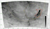 |
Fig. 1 Stereographic projection of the multi-resolution gas column density map of CrA and its surroundings from Herschel and Planck (named |

![Mathematical equation: $N_{\textrm{H}_2} \,{\approx}\,0.5\,{\times}\, N_{\textrm{H}}\, [\textrm{cm}^{-2}]$](/articles/aa/full_html/2020/12/aa39282-20/aa39282-20-eq68.png)
2 The surroundings of the CrA molecular cloud
The CrA molecular cloud is an ongoing star-forming region located at a distance of (156 ± 9) pc (Dzib et al. 2018; Galli et al. 2020; Zucker et al. 2020). Both Planck and Herschel far-infrared and submillimeter data have revealed the full dynamic range of dust emission around CrA (Planck Collaboration XXV 2011; Bresnahan et al. 2018). Bresnahan et al. (2018) found a selection of prestellar cores, protostars, and young stellar objects (YSOs) located both along dense molecular filaments, as also observed in most Gould-Belt clouds (e.g., André et al. 2010; Könyves et al. 2015, 2020; Bracco et al. 2017), and within the Coronet cluster, in the northern tip of CrA. Analyzing the column density map of molecular gas,  , derived from Herschel data, the authors also found that the morphology of the filamentary structures is asymmetric between the eastern and the western portions of CrA, suggesting external influence on the cloud shape.
The scenario for the formation of CrA has been long disputed for long time. Neuhäuser & Forbrich (2008) suggested that the cloud was produced by the infall of a high-velocity cloud into the Galactic plane, while Mamajek & Feigelson (2001) and de Geus (1992) claimed that CrA could be the result of the expansion of a superbubble coming from the Upper Centaurus Lupus association.
Regardless of the exact physical origin, however, all scenarios include the presence of an external source of compression onto CrA. In Fig. 1, we show a large panorama of the column-density map of CrA. This map combines Planck and Herschel Gould Belt survey data giving rise to a wide dynamic range of densities, from the most diffuse ISM ( < 1019 cm−2) traced by Planck at an angular resolution of 5′, to the densest regions in CrA (
 > 1021 cm−2) at an angular resolution of18′′ with Herschel. The region covered by the high resolution of Herschel is contained within the red contour in Fig. 1. More details about this map, hereafter called
  (the superscript “C” stands for “combined”), are provided in Appendix A, where blow-ups of CrA are shown as well as the Coronet cluster, labeled as CrA-A in Fig. A.1. Although for column densities less than 1021 cm−2 it would be probably more appropriate to refer to
  , to be consistent with the conventions used in this work for the dust continuum emission (see Appendix A) we kept the
  notation.
The  map reveals a continuous stretch of diffuse dusty features that extend over tens of degrees in the sky toward CrA (see the solid red contour) along two curved lines (see the dashed yellow lines) tracing shell-like structures, hereafter C.1 and C.2, respectively. The association between these two curves and the morphology of CrA is precisely the subject of this work.
3 CrA at the intersection of two HI shells
In this section we describe the spectroscopic properties and the distance of C.1, C.2, and CrA.
3.1 Spectroscopic data of C.1, C.2, and CrA
Diffuse dust emission has been known for long to be tightly coupled with the multiphase HI gas (e.g., Burstein & Heiles 1982; Boulanger et al. 1996; Lenz et al. 2017). We explored the HI spectroscopic data cubes at 21 cm of the surroundings of CrA from the third data release of the Galactic All Sky HI Survey1 (GASS; McClure-Griffiths et al. 2009; Kalberla et al. 2010). These data have an angular resolution of 16′, a spectral resolution of 1 km s−1, and a mean noise level of ~50 mK (Kalberla & Haud 2015).
The CrA molecular cloud is known to have a systemic velocity of ~5 km/s in the local standard of rest, Vlsr. As shown by Yonekura et al. (1999), using spectra of carbon-monoxide isotopes (C18 O) from the NANTEN telescope, velocities of CrA range between 3.5 and 7.5 km s−1. Inspecting the GASS HI data we noticed an astonishing correlation between the diffuse dusty structures seen in Fig. 1 and the HI emission detected at two velocities of 3.3 (blueshifted) and 7.4 km s−1 (redshifted),in the same velocity range of CrA.
Figure 2 is a RGB image that combines together the two HI components, in blue and red, and the  map in green. The morphological correspondence between C.1 and C.2 with the intensity of HI in the two velocity channels is striking.
In projection, CrA appears to be close to the intersection of the HI intensities of C.1 and C.2, which may correspond to a receding and approaching velocity components, respectively. Both HI components resemble to shells that were already discovered and discussed in Moss et al. (2012) and Thomson et al. (2018). Moss et al. (2012) also showed that HI emission is not only limited to the above-mentioned velocity channels but it is rather spread between 3 and 11 km s−1 (see their Fig. 2). Notwithstanding, the authors never highlighted the apparent association of the two shells with CrA. This was only briefly mentioned by Thomson et al. (2018), who, however, did not provide any quantitative analysis. Based on Galactic rotation models, Moss et al. (2012) had estimated the distance of the HI component of C.1 to be on the order of 1.5 kpc, which made absolutely impossible the physical connection of the shell with CrA. However, we notice that the projected morphology and the commonvelocity range at which both the HI shells and CrA appear, already suggest the likely association between the atomic and molecular phases, although no CO is detected toward either of the shells within 15 degrees from CrA (Dame et al. 1987, 2001).
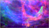 |
Fig. 2 RGB image showing HI emission at 7.4 km s−1 (red), the |

3.2 A new distance estimate
We here strengthen the physical association of CrA with the HI shells revising the estimates of their distance using guidelines from dust extinction Gaia data (e.g., Luri et al. 2018).
We estimated the distance toward portions of both shells and CrA by assessing the increase of extinction in the G band (AG) as a function of their parallax distance (see also Yan et al. 2019). The distance analysis performed in this work will be thoroughly detailed in Palmeirim et al. (in prep.). We describe the basic methodology. The method is based on the expected statistical increment of AG of Gaia background stars toward regions where dust extinction is significant. We selected a sample of 1 826 578 Gaia DR2 stars with parallax uncertainties below 20%, distances up to 2 kpc distance, and AG estimates that cover the entire field of view of the  map.
map.
We note that the mean AG value of the distributions of extinction as a function of the distance is not a reliable estimator, since these distributions can suffer from strong biases with typical uncertainty of ~0.4 mag (see Andrae et al. 2018 for more details). The AG distributions are better represented by their median value as estimated by bootstrapping the data with bins of 30 sources (hereafter these median values will be noted with the superscript “bs”).
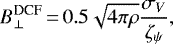
The sample of Gaia sources used to estimate the distance for each region was defined based on a column density threshold on  . The choice of the threshold value was based on the best compromise between having a significantly large statistical sample of sources while, at the same time, not contaminating the sample with too many sources with low AG, which would in effect decrease the amplitude of the AG jumps (see Yan et al. 2019 for more on the threshold selection). Taking these considerations into account, we defined a column density thresholds of 7 × 10²⁰ and 3 × 1020 cm−2 for CrA and for the shells, respectively. In Fig. 3 we show on top of the AG map the selected regions for C.1, C.2, and CrA, in red, blue, and green, respectively.
By analysing the behavior of  between the on- and off-cloud (in gray in Fig. 3) samples, we could easily identify at which distances the dust extinction was significant. As demonstrated in Fig. 4, all three regions show a significant increment of
  at ~150 pc, when compared with the flat off-cloud sample.
In the case of CrA, most of the  increment seems to be at ~150 pc, however, there is another less prominent increase in A
 at ~340 pc (see Fig. 5). To analytically describe the increases in AG, we fit a smoothed step function to the A
 as a function of their respective bootstrapped distance (dbs) with the following form:
 (1)
(1)
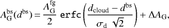
where A is the constant AG value of the foreground sources, ΔAG is the AG increment, dcloud is the distance of the extinction increase, erfc is the complementary error function used to smooth the step and σd is the standard-deviation of a normal Gaussian distribution, the error on the distance estimate, which also gives a relative representation of the region thickness. The fitted values for each region are displayed in Table 1, and the estimated distances are marked in Fig. 4. For the off-cloud sample we found a mean
  value of 0.25 and a standard deviation of σoff = 0.06 mag (obtained using the 104 243 sources where the column density was less than 6.5 × 1019 cm−2). We considered as significant jumps in
  all increments with ΔAG at least 3σoff, or 0.18 mag. In Fig. 4 the best-fit
  curves are over-plotted on the data as solid lines.
The obtained distance toward CrA of (150.5 ± 6.3) pc is consistent with the most recent distance estimates (e.g., Zucker et al. 2020), while the shells seem to enclose CrA within a distance range between ~140 and ~190 pc. We notethat no evidence was found for the presence of extinction at the estimated kinematic distance of 1.5 kpc derived from Moss et al. (2012) for none of the shells (see Fig. 5). In conclusion, we found that portions of C.1 and C.2 are located at a similar distance as CrA and, therefore, very likely physically connected to it.
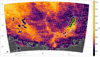 |
Fig. 3 Surface density map in galactic coordinates of the median AG values of the sample of 1 826 578 Gaia DR2 stars covering the same field of view as Fig. 1. The positions of the Gaia sources used to estimate the distance of CrA, C.1 and C.2, are overlaid in green, red (with white contours) and blue, respectively. The off position is shown in gray. CrA, C.1, and C.2 are shown as in Fig. 1. |
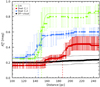 |
Fig. 4 Median |


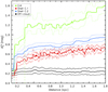 |
Fig. 5 Median |

 |
Fig. 6 Magnetic-field morphology of the C.1 shell. Comparison between Planck polarization data (top row) and the Stokes parameters produced with a toy model (bottom row) describing the magnetic-field geometry compressed on the surface of a shell seen in projection (in yellow). Units and dynamic range in both rows are the same. Top right panel: we overlay on the polarization-fraction map (right panel) black contours of HI emission at 30, 35, 40, 45, and 50 K tracing the 7.4 km s−1 component of C.1 (dashed-line circle in all panels). The position of the CrA molecular cloud is shown with white (left and right panels) and gray (central panels) contours of
|

4 Magnetic-field properties
We here describe the magnetic-field properties of the shells and CrA.
4.1 Magnetic-field geometries
Additional evidence of the physical association between CrA and C.1, or C.2, comes from the magnetic-field structure projected on the plane of the sky inferred from the Planck polarization data of interstellar dust emission at 850 μm. In the top row of Fig. 6 we show maps of the Stokes parameters, I, Q, U, and the polarization fraction, defined as 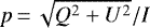 , in the surroundings of CrA and C.1. We show maps smoothed to 30′, using the ismoothing routine in HEALPix2, in order to increase the signal-to-noise ratio in polarization at the intermediate latitudes of CrA. Planck Collaboration Int. XXXV (2016) and Soler (2019) already discussed the statistics of the relative orientation between the structures of the magnetic field and that of matter density in CrA. They found that most of the molecular gas appears elongated along the magnetic-field lines except for the densest region, where the Coronet cluster is located (see yellow arrow in Fig. 6). Moreover, CrA shows a clear perpendicular configuration with respect to the mean magnetic-field orientation in its surroundings. This can be also seen in the top-left panel of Fig. 6, where on top of the Stokes I map we overlaid the position of CrA and the magnetic-field lines from Planck data3. The magnetic-field orientation also traces the curvature of the lower part of the shell corresponding to C.1. This is shown in the top-right panel of the figure, where we show superposed on the p map black contours of HI intensity at Vlsr = 7.4 km s−1 between 30 and 50 K with steps of 5 K. The association between the HI emission of C.1 and the increase in p up to more than 10% is evident.
On the bottom row of Fig. 6, we show synthetic Stokes parameters derived from a purely geometrical toy model of a magnetic field compressed on the surface of a shell seen in projection (Krumholz et al. 2007; Planck Collaboration Int. XXXIV 2016). Our model is static and it includes an horizontal background/initial magnetic-field orientation and a magnetic-field component perfectly following the edges of a shell, which, in our simplified scheme, is generated by a central explosion. From left to right in the bottom of Fig. 6, we show the analog maps as in the top row but for the model. Our toy model, shown with the same units and dynamic range as that of the data, is made of a linear combination of the Stokes parameters derived from the uniform background magnetic-field orientation (horizontal) and those of the magnetic-field component completely confined to the surface of the shell and following its curvature. The resulting synthetic Stokes Q and U parameters of dust polarization are only determined by the structure of the projected magnetic-field (see Eq. (1) in Bracco et al. 2019). We do not consider any contribution to the Planck polarization due to change in dust grain properties (Hoang et al. 2018); we normalize the modeled Stokes parameters to the polarization fraction of 10% seen in the data.
Despite the simplicity of our spherical model, we can recognize some common features with the Planck polarization data. The variation from positive to negative (red and blue) values of Q and U, as well as the enhancement of the p map in its bottom part due to coherence of magnetic-field orientations along the line of sight resemble well the patterns observed at large scale in the data. Although our symmetric and sperical model does not capture the full complexity and inhomogeneity of the observed Stokes parameters, it suggests that CrA and C.1 belong to a single magnetized structure associated to the HI shell.
As for C.2, in Fig. 7 we show the corresponding Stokes parameters from the Planck data with intensity contours tracing the dust continuum emission of the shells. In this case the analogy between the simple toy model and the polarization data is less straightforward. This is mostly because C.2 extends over a very large area in the sky, where the line-of-sight confusion in polarization becomes important. Our simplified geometrical model is certainly not suited to describe such wide sky areas. We note, however, that an alternation in sign for both Q and U can be roughly observed also for C.2, suggesting that even C.2 and CrA may be part of a single large-scale magnetized shell-like structure.
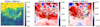 |
Fig. 7 Stereographic projection of Stokes I, Q, and U parameters(from left to right) from Planck observations showing the large view around the C.2 shell as traced by the ochre circle. A grid of Galactic coordinates is shown in the left panel with steps of 5° both in longitude (between −5° and +35°) and in latitude (between −40° and −5°). In all three panels Stokes I contours at 0.5, 0.6 and 1 MJy sr−1 are shown. |
4.2 Magnetic-field strengths
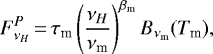
The ordered magnetic-field responsible for the peak of p in the data is possibly the result of shock compression (Ntormousi et al. 2017). Under this hypothesis we considered the lower section of C.1 as the best suited location to witness the original shell compression, as CrA already evolved into a star-forming region. Focusing on this lower section of C.1 (see red box in the top panel of Fig. 8), which possibly corresponds to the intersection with C.2 (see Fig. 2), we estimated the plane-of-the-sky magnetic-field strength, B⊥, using the Davis-Chandrasekhar-Fermi (DCF) method in the HI gas. The DCF method provides an estimate of B⊥ under the assumption that the magnetic field is frozen into the gas and that the dispersion of the local magnetic-field orientation is due to transverse and incompressible Alfvén waves. B⊥ depends on the density of the gas (ρ in units of g cm−3), the turbulent dispersion of the line-of-sight velocity (σV in units of cm s−1), and the dispersion of polarization angles (ζψ in radians), as follows
 (2)
(2)
where we included the correction factor of 0.5 from Ostriker et al. (2001).
The HI medium is a bi-stable gas composed of warm neutral medium (WNM), at temperatures of ~8000 K and number densities of ~0.3 cm−3, and cold neutral medium (CNM) with corresponding temperatures and densities of ~50 K and ~50 cm−3, respectively (Field 1965; Wolfire et al. 2003). In this work we focused on the contribution to the HI spectra from the CNM only, as the structure of the CNM, rather than that of the WNM, was found strongly correlated with magnetic fields traced by dust polarization both in highly filamentary structures of thin HI emission, called fibers (Clark et al. 2015, 2019), and in the diffuse ISM at intermediate and high Galactic latitude (Planck Collaboration Int. XXXII 2016; Ghosh et al. 2017; Adak et al. 2020).
In order to estimate ρ and σV for the CNM, we performed a Gaussian decomposition analysis of the multiphase HI spectra using the Regularized Optimization for Hyper-Spectral Analysis (ROHSA)4 algorithm described in Marchal et al. (2019). The basic principle of ROHSA is to decompose HI spectra into a linear combination of Gaussian spectral lines. The novelty of this technique, compared to all previous analogs in the analysis of spectroscopic data (e.g., Nidever et al. 2008; Martin et al. 2015; Miville-Deschênes et al. 2017; Riener et al. 2019), is that it imposes a spatial coherence across the field of view in the determination of the parameters of the Gaussian spectral decomposition. All spectra are fit at the same time based on a multi-resolution approach, dividing the original field of view from coarse to fine grids. To make sure that the recovered Gaussian parameters are spatially smooth, specific regularization terms are added. ROHSA performs a regression analysis using a regularized nonlinear least-square criterion.
In Fig. 9 we show an example of how ROHSA works. It is possible to see the input HI spectrum from GASS in orange and the reconstructed spectrum based on the Gaussian model from ROHSA in gray. We stress again that, although for each line of sight the solution may be degenerate, the advantage of ROHSA is to reduce the uncertainty of the model by looking for spatial coherence of the Gaussian solution across the field of view. We used a twelve-Gaussian decomposition. As recommended in Marchal et al. (2019), this value (NG = 12) is empirically chosen to converge toward a noise-dominated residual of the model. It is important to note that due to regularization, the number of Gaussians for an individual line of sight is always smaller than NG. The spatial coherency of ROHSA of the fitted parameters prevents the data from being over-fitted with the NG Gaussians available (Marchal et al. 2019).
The Gaussians differ because of their standard deviation, σG. We isolated the CNM from the WNM component imposing limits on σG, such that Gaussians are associated to CNM if σG < 3 km s−1 (see light-blue curves in Fig. 9) and to WNM in the opposite case (Marchal et al. 2019). In Fig. 9 the thick blue and red lines correspond to the full HI CNM and WNM components, respectively, derived with ROHSA.
We averaged all the σGi of the CNM Gaussians weighted on their corresponding column density (NHi from Eq. (B.1) in Soler et al. 2018) within the red box shown in Fig. 8 as
 (3)
(3)
where N is the number of lines of sight within the red box. We obtained σobs = 1.5 × 105 cm s−1. This quantity corresponds to the observed velocity dispersion of the CNM component. This is also equivalent to 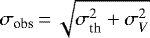 , or the sum of the thermal and turbulent velocity dispersions in the CNM. In order to extract σV, we made the reasonable assumption that the sonic Mach number,
  , of the CNM is 3 ± 1 (i.e., Heiles & Troland 2003; Murray et al. 2015). Cs is the adiabatic sound speed defined as
  , where T is the gas temperature, kB the Boltzmann’s constant, and μ = 1.4 the mean atomic weight. Given the adiabatic index of a monoatomic gas, γ = 5∕3, we got
 (4)
(4)
where the error mostly depends on the value of Ms. We also provided a rough estimate for the temperature of the CNM gas equal to 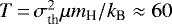 K.
K.
Assuming optically thin HI emission at the intersection of the shells, we computed the density as ρ =  , where μ = 1.4 is the mean molecular weight and estimated the column density, NH, averaged within the red box in Fig. 8. We obtained NH = (3.7 ± 0.4) × 1020 cm−2. We also notice that NH in Fig. 8 better shows the east rim of the C.1 shell compared to
  .
.
The CNM thickness L along the line of sight at the intersection of the shells was estimated in two ways. We first accounted for a line-of-sight thickness similar to the plane-of-the-sky linear dimension of the red box of 1.5°, which, at the distance of 150 pc, corresponds to 4 pc. Second, we considered the region as part of a sheet-like structure such that, given the value of NH reported above, the number density of CNM was greater than 10 cm−3 but smaller than 100 cm−3, or the critical density for CO formation, as CO was not detected by Dame et al. (1987, 2001) toward the same region (see Sect. 3). We obtained an upper limit to the line-of-sight thickness equal to 12 pc. These two line-of-sight thicknesses produced densities of 31 and 10 cm−3, respectively. We also notice that these two values of L are consistent with the estimate of σd obtained for C.1 in Sect. 3.2.
As for the dispersion of polarization angles, ζψ, we applied the same methodology described in Appendix D of Planck Collaboration Int. XXXV (2016) using the Stokes parameters Q and U as follows,
![Mathematical equation: \begin{equation*}\zeta_{\psi}\,{=}\,\sqrt{\left\langle\, \left[\, \frac{1}{2}\tan^{-1}{(Q\langle U \rangle - U\langle Q \rangle, Q\langle Q \rangle + U\langle U \rangle })\,\right]^2\,\right\rangle}, \end{equation*}](/articles/aa/full_html/2020/12/aa39282-20/aa39282-20-eq31.png) (5)
(5)
where ⟨...⟩ denotes the average over the pixels in the red box of Fig. 8. We used the version of the inverse tangent function with two signed arguments to resolve the π ambiguity in the definition of ψ, as it corresponds to orientations and not directions. We obtained ζψ = (6.1 ± 0.6) × 10−2 radians (~3.5°). This value was recovered as follows. Instead of using Eq. (D.11) in Planck Collaboration Int. XXXV (2016) to derive the error on ζψ, we preferred evaluating the impact on it of changes in the Planck angular resolution. We estimated ζψ varying the angular resolution of the Planck polarization data from 20′ to 30′ and 40′. Hence, we averaged and took the corresponding standard deviation using Eq. (5).
Averaging the above spectroscopic and polarization data in the 5.5-deg2 red box in Fig. 8, we obtained a mean value of  equal to (27 ± 8) μG, where the error mostly depends on the choice of L. We reportedthe value obtained as the mean and the maximum error of the two magnetic-field strengths obtained with the limits in the line-of-sight thickness of the shell of 4 and 12 pc detailed above.
For comparison, we also estimated  off of the shells, in the two yellow boxes shown in Fig. 8 and labeled “north” and “south”. The north box was taken to be as far as possible from C.1 and not contaminated by other large-scale patterns in polarization. Since in these cases the line-of-sight thickness is even less constrained than before we provided only upper limits to the corresponding magnetic-field strengths using the longest line-of-sight thickness of 12 pc. We obtained magnetic-field strengths of < 6 μG and < 12 μG for the north and south box, respectively. We notice that the error reported for the value of
  in the red box may be in fact underestimated due to the multiple assumptions made to apply the DCF method. However, we stress that it is significant the relative comparison between the values of
  found in theyellow boxes with that obtained in the red box.
Finally, we also attempted to estimate the magnetic-field strength in CrA. Planck Collaboration Int. XXXV (2016) already provided an estimate of  between 5 and 12 μG toward CrA. However, we believe that a mean volume density of ~100 cm−3 used in the previous analysis is significantly underestimated for CrA. Using the
  map we were able to reach a mean column density as high as 3 × 1021 cm−2 in the region labeled as CrA-A in Fig. A.1. Given a line-of-sight thickness of ~0.4 pc (10′, the plane-of-the-sky width, at a distance of 150 pc) we obtained an estimate of nH ≈ 4500 cm−3. The value of ζψ toward CrA is about 50° (consistent both at 5′ and 10′ angular resolution), as also reported in Planck Collaboration Int. XXXV (2016). Considering a similar σV of 0.6 km s−1 as in the previous analysis we obtained an estimate of
  in CrA between 33 and 80 μG, a factor of ~7 larger than what previously claimed. However, we stress that because of the very large value of ζψ the use of the DCF method in CrA is highly unreliable (Ostriker et al. 2001). This is possibly caused by the fact that CrA already turned into a star-forming region, where the magnetic-field structure could be affected by the self-gravity of the cloud, possibly undergoing large-scale gravitational collapse.
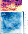 |
Fig. 8 Top panel: blow-up of the p map shown in the top-right panel of Fig. 6 showing in more detail the red box where weestimated the magnetic-field strength of the C.1 shell. Bottom panel: column density map, NH, of the CNM isolated with ROHSA. This is the same field of view shown in Fig. 6. Beside the red box shown in the top panel we also indicate two yellow boxes where we estimate the magnetic-field strength and compare it with C.1. |
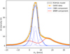 |
Fig. 9 Example of Gaussian decomposition of ROHSA for one given line of sight in the red box of Fig. 8. GASS data are shown in orange, the reconstructed modeled spectrum from ROHSA is shown in gray shade, the total CNM component is shown in blue, and the WNM component in red. Light-blue curves represent the multiple Gaussians associated with the CNM from ROHSA. |
5 Discussion
Despite the many assumptions and large uncertainties related to the estimate of  , its large value found at the intersection of C.1 and C.2 suggests an unusual magnetic-field strength in the CNM. It is at least a factor of two larger than what we obtained off of the shells. Moreover, based on Zeeman splitting observations, magnetic fields in the CNM are normally on the order of a few μG, with a median value of (6 ± 2) μG (Heiles & Troland 2003, 2005; Crutcher et al. 2010; Crutcher 2012). Thomson et al. (2018) studied the line-of-sight magnetic-field structure and strength of the C.1 shell. They concluded that their ~ 2 μG line-of-sight magnetic field is compatible with a magnetic-field structure contained on the surface of a shell but with a strong magnetic-field component on the plane of the sky.
Large magnetic-field strengths were already observationally found in the vicinity of several interstellar superbubbles that are the result of large-scale shocks produced by clustered feedback of young OB star associations or supernova explosions (McClure-Griffiths et al. 2006; Soler et al. 2018). MHD numerical simulations have shown how these supersonic motions can trigger molecular-cloud formation and how the presence of magnetic fields may strongly affect the resulting structure of the shocked-multiphase ISM (e.g., Ntormousi et al. 2017). In particular, Ntormousi et al. (2017) illustrated that magnetic pressure causes the shell of a single expanding bubble to thicken in density perpendicular to the mean-field direction while structuring less parallel to it. This is also advocated by Inutsuka et al. (2015) that proposed a scenario in which molecular clouds form as the consequence of multiple supersonic compressionfrom interacting shells, or bubbles, mostly happening along the direction of the local interstellar magnetic field.
We believe that our observational case supports this scenario in which the formation of the CrA molecular cloud would have most likely occurred in regions where the shell expansion coincides with the mean-magnetic field direction. If so, we would also expect less formation of molecular gas and an increase of the magnetic-field strength triggered by the shell compression in the opposite direction. This is possibly the right interpretation for the large value of  in the CNM as traced by HI gas only toward the intersection of C.1 and C.2. The lower values of
  obtained further away from the shell compression – in the north and south boxes – which are rather consistent with the usual values of the diffuse magnetized CNM, also strengthen this scenario.
In order to confirm this interpretation of compressed magnetized gas caused by interstellar bubbles in the proximity of CrA, we encourage future observations of Zeeman splitting of HI and hydroxyl (OH) that might directly measure the magnetic-field strength both in the CNM of the shell and in the translucent parts of the molecular cloud, respectively.
6 Conclusions
We reported the unprecedented association of the Corona Australis molecular cloud (CrA), a close-by star-forming region, with two shell-like structures (C.1 and C.2) that span tens of degrees in the sky seen in dust emission and polarization, and in spectral-line observations of atomic hydrogen (HI) at 21 cm.
Although the shells were already known, their physical association with CrA was never suggested before. Based on the analysis of dust-extiction data from Gaia, we localized the distance of the shells between 140 and 190 pc in the environs of CrA (150 ± 6 pc), significantly revising the first estimate of their distance of about 1.5 kpc by Moss et al. (2012). A more detailed discussion of the 3D configuration of CrA and the shells will be soon presented in a follow-up paper by Palmeirim et al. (in prep.).
We also analyzed dust continuum emission and polarization data from Herschel and Planck to constrain the magnetic-field structure of both CrA and the shells. Both C.1 and C.2 showed coherent polarization patterns with CrA, strongly suggesting a common belonging to the same magnetized structure, possibly the compressed front of an expanding bubble, where the molecular cloud would have formed in a compressed layer along the mean magnetic-field orientation. Focusing on the intersection region between C.1 and C.2, we estimated the magnetic-field strength in the compressed gas applying the Davis-Chandrasekhar-Fermi method to the cold neutral medium extracted from the HI spectra and to the Planck polarization data. We obtained a magnetic-field strength of (27 ± 8) μG. This is a large value, at least a factor of two larger than the upper limits that we obtained off of the shells of < 6 and < 12 μG. This result is an additional indication of the presence of an external compression on the shells that may have locally increased the strength of the magnetic field, as also shown by other known magnetized superbubbles.
Our work supports a scenario of molecular-cloud formation triggered by supersonic compression of interstellar matter and of the frozen-in magnetic field from interacting bubbles in the ISM.
Acknowledgements
We would like to thank the anonymous referee for the valuable comments that improved the content of this work. We thank V. A. Moss, S. Inutsuka, and J.-Ph. Bernard for useful discussions on the properties of the HI shells and on the derivation of the Planck offsets for Herschel. A.B. acknowledges the support from the European Union’s Horizon 2020 research and innovation program under the Marie Sk?odowska-Curie Grant agreement No. 843008 (MUSICA). This work has received support from the European Research Council under the European Union’s Seventh Framework Programme (ERC Advanced Grant Agreement no. 291294 – “ORISTARS”) a from the French national programs of CNRS/INSU on stellar and ISM physics (PNPS and PCMI). P.P. and D.A. acknowledge support from FCT/MCTES through Portuguese national funds (PIDDAC) by grant UIDB/04434/2020. P.P. receives support from the fellowship SFRH/BPD/110176/2015 funded by FCT (Portugal) and POPH/FSE (EC) and by a STSM Grant from the EU COST Action CA18104: MW-Gaia. This work made use of the JBIU IDL library, available at http://www.simulated-galaxies.ua.edu/jbiu/.
Appendix A Using Planck and Herschel data to derive multi-resolution column density maps
In this section we describe the methodology employed to generate the  map shown in Fig. 1, or the column density map that combines Planck and Herschel data reaching a suitable compromise between high angular resolution in the dense ISM and high sensitivity in the diffuse ISM. The data can be downloaded at http://pla.esac.esa.int/ and http://gouldbelt-herschel.cea.fr/archives/. Here we detail the general strategy of our method, already applied in Bresnahan et al. (2018), Ladjelate et al. (2020), and Könyves et al. (2020) to analyze column densities of molecular clouds observed within the Herschel Gould Belt Survey (André et al. 2010). The strategy that follows can be applied to more general cases.
Our first aim was to correct Herschel far-infrared fluxes at frequency ν,  , for their zero levels using Planck data as a reference. The Herschel bands that we considered were at 160, 250, 350, and 500 μm. The Planck observations, however, did not cover the full range of Herschel wavelengths, but only the long-wavelength channels (>350 μm, Planck Collaboration I 2016). Inspired by the methodology introduced in Bernard et al. (2010), we interpolated the Planck fluxes in the Herschel bands,
  , using a modified blackbody spectrum for dust emission in the optically thin regime, such as
 (A.1)
(A.1)
where τ is the dust optical depth along the line of sight, β is the dust emissivity index, Bν is the Planck function of blackbody spectrum, and T is the temperature of the dust grains. The subscript “m” refers to the parameters of dust emission derived at 850 μm from the all-sky dust model presented in Planck Collaboration XI (2014). The maps of these parameters, downloadable at the link above, were obtained from fitting a modified blackbody to the Planck data between 350 and 850 μm, and IRAS data at 100 μm. As discussed by the authors the angular resolution of the full-sky parameter maps is not uniform: τm and Tm are at 5′, while βm is at 30′.
Once obtained  from Eq. (A.1), we smoothed and degraded the Herschel flux maps to the Planck beam of 5′ and pixel resolution of 1.7′. A simple linear regression between
  and the degraded
  in the common observed sky areas allowed us to retrieve the offsets to set the zero levels of the Herschel maps with a precision better than 10%.
Our second step was to obtain column density maps from well calibrated fluxes, knowing that τν = κνΣ, where κν is the dust opacity and Σ the gas surface density. The latter can be written as  , which depends on the mean molecular weight
  , on the mass of the hydrogen atom mH, and on the column density
  .
.
Using both  and
and  we re-derived, through a modified blackbody fit to the fluxes between 160 and 500 μm, the dust emission parameters both for Herschel and Planck data. In both cases we assumed β = 2 and
  cm2 g−1 (André et al. 2010; Roy et al. 2014; Könyves et al. 2015; Bracco et al. 2017).
The fitting procedure enabled us to separately obtain, but in a consistent way, both  at 5′ and
  at 36′′, where the superscripts P and H stand for Planck and Herschel, respectively. Finally, implementing the technique described in Appendix A of Palmeirim et al. (2013), we also obtained the high-resolution
  at 18′′. In short, the latter was obtained expressing the gas surface density at 250 μm, Σ250, as a sum of three terms:
 (A.2)
(A.2)
where Σ500, Σ350, and Σ250 represent smoothed versions of the intrinsic gas surface density distribution after convolution with the Herschel SPIRE beam at 500, 350, and 250 μm, respectively. We combined  with
with  producing
  , as follows
 (A.3)
(A.3)
where the sign “*” represents the convolution of  with a Gaussian beam of 5′ angular resolution.
Other works have delivered methodologies to combine Planck and Herschel data (e.g., Lombardi et al. 2014; Abreu-Vicente et al. 2017). We believe that our method has two advantages: 1) the derivation of column-density maps from the two datasets in a completely consistent way; 2) the production of higher-resolution (18′′ vs. 36′′) maps in the areas imaged with Herschel.
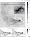 |
Fig. A.1 Herschel-Planck |


In Fig. A.1 we show a blow-up of the  map (see Fig. 1) in the surroundings of CrA in Celestial coordinates. This blow-up image shows a multi-resolution map with the part at 18′′ resolution inside the black rectangle and the part at 5′ resolution elsewhere. This map allows one to appreciate the large dynamic range in column density of the combined map. Combining large and small angular scales with Planck and Herschel data, respectively, we are able to study the large-scale environment of the molecular cloud without loosing the richness of the detailed density structure where star formation is acting in CrA (see the red contour encircling the Coronet cluster labeled as CrA-A). The two bottom panels in Fig. A.1 show
  (left) and
  (right) with a stretch in gray scale that highlights the limits of the Planck resolution in probing the internal regions of CrA that are conversely highly detailed by Herschel.
References
- Abreu-Vicente, J., Stutz, A., Henning, T., et al. 2017, A&A, 604, A65 [CrossRef] [EDP Sciences] [Google Scholar]
- Adak, D., Ghosh, T., Boulanger, F., et al. 2020, A&A, 640, A100 [CrossRef] [EDP Sciences] [Google Scholar]
- Andrae, R., Fouesneau, M., Creevey, O., et al. 2018, A&A, 616, A8 [NASA ADS] [CrossRef] [EDP Sciences] [Google Scholar]
- André, P., Men’shchikov, A., Bontemps, S., et al. 2010, A&A, 518, L102 [NASA ADS] [CrossRef] [EDP Sciences] [Google Scholar]
- André, P., Di Francesco, J., Ward-Thompson, D., et al. 2014, Protostars and Planets VI, eds. H. Beuther, R. S. Klessen, C. P. Dullemond, & T. Henning (Tucson, AZ: University of Arizona Press), 27 [Google Scholar]
- Arzoumanian, D., André, P., Könyves, V., et al. 2019, A&A, 621, A42 [NASA ADS] [CrossRef] [EDP Sciences] [Google Scholar]
- Ballesteros-Paredes, J., André, P., Hennebelle, P., et al. 2020, Space Sci. Rev., 216, 76 [CrossRef] [Google Scholar]
- Bernard, J. P., Paradis, D., Marshall, D. J., et al. 2010, A&A, 518, L88 [NASA ADS] [CrossRef] [EDP Sciences] [Google Scholar]
- Boch, T., & Fernique, P. 2014, ASP Conf. Ser., 485, 277 [Google Scholar]
- Boulanger, F., Abergel, A., Bernard, J. P., et al. 1996, A&A, 312, 256 [Google Scholar]
- Bracco, A., Palmeirim, P., André, P., et al. 2017, A&A, 604, A52 [NASA ADS] [CrossRef] [EDP Sciences] [Google Scholar]
- Bracco, A., Candelaresi, S., Del Sordo, F., & Brandenburg, A. 2019, A&A, 621, A97 [NASA ADS] [CrossRef] [EDP Sciences] [Google Scholar]
- Bresnahan, D., Ward-Thompson, D., Kirk, J. M., et al. 2018, A&A, 615, A125 [NASA ADS] [CrossRef] [EDP Sciences] [Google Scholar]
- Burstein, D., & Heiles, C. 1982, AJ, 87, 1165 [NASA ADS] [CrossRef] [Google Scholar]
- Chevance, M., Kruijssen, J. M. D., Vazquez-Semadeni, E., et al. 2020, Space Sci. Rev., 216, 50 [CrossRef] [Google Scholar]
- Clark, S. E., Hill, J. C., Peek, J. E. G., Putman, M. E., & Babler, B. L. 2015, Phys. Rev. Lett., 115, 241302 [NASA ADS] [CrossRef] [Google Scholar]
- Clark, S. E., Peek, J. E. G., & Miville-Deschênes, M. A. 2019, ApJ, 874, 171 [NASA ADS] [CrossRef] [Google Scholar]
- Crutcher, R. M. 2012, ARA&A, 50, 29 [NASA ADS] [CrossRef] [Google Scholar]
- Crutcher, R. M., Wandelt, B., Heiles, C., Falgarone, E., & Troland, T. H. 2010, ApJ, 725, 466 [NASA ADS] [CrossRef] [Google Scholar]
- Dame, T. M., Ungerechts, H., Cohen, R. S., et al. 1987, ApJ, 322, 706 [NASA ADS] [CrossRef] [Google Scholar]
- Dame, T. M., Hartmann, D., & Thaddeus, P. 2001, ApJ, 547, 792 [NASA ADS] [CrossRef] [Google Scholar]
- Dawson, J. R., McClure-Griffiths, N. M., Wong, T., et al. 2013, ApJ, 763, 56 [NASA ADS] [CrossRef] [Google Scholar]
- Dawson, J. R., Ntormousi, E., Fukui, Y., Hayakawa, T., & Fierlinger, K. 2015, ApJ, 799, 64 [NASA ADS] [CrossRef] [Google Scholar]
- de Geus, E. J. 1992, A&A, 262, 258 [NASA ADS] [Google Scholar]
- Dzib, S. A., Loinard, L., Ortiz-León, G. N., Rodríguez, L. F., & Galli, P. A. B. 2018, ApJ, 867, 151 [NASA ADS] [CrossRef] [Google Scholar]
- Field, G. B. 1965, ApJ, 142, 531 [NASA ADS] [CrossRef] [Google Scholar]
- Galli, P. A. B., Bouy, H., Olivares, J., et al. 2020, A&A, 634, A98 [CrossRef] [EDP Sciences] [Google Scholar]
- Ghosh, T., Boulanger, F., Martin, P. G., et al. 2017, A&A, 601, A71 [NASA ADS] [CrossRef] [EDP Sciences] [Google Scholar]
- Heiles, C., & Troland, T. H. 2003, ApJ, 586, 1067 [NASA ADS] [CrossRef] [Google Scholar]
- Heiles, C., & Troland, T. H. 2005, ApJ, 624, 773 [NASA ADS] [CrossRef] [Google Scholar]
- Heitsch, F., & Putman, M. E. 2009, ApJ, 698, 1485 [NASA ADS] [CrossRef] [Google Scholar]
- Hennebelle, P., & Falgarone, E. 2012, A&ARv, 20, 55 [NASA ADS] [CrossRef] [Google Scholar]
- Hennebelle, P., & Inutsuka, S.-i. 2019, Front. Astron. Space Sci., 6, 5 [NASA ADS] [CrossRef] [Google Scholar]
- Hoang, T., Cho, J., & Lazarian, A. 2018, ApJ, 852, 129 [NASA ADS] [CrossRef] [Google Scholar]
- Inutsuka, S.-i., Inoue, T., Iwasaki, K., & Hosokawa, T. 2015, A&A, 580, A49 [NASA ADS] [CrossRef] [EDP Sciences] [Google Scholar]
- Joubaud, T., Grenier, I. A., Ballet, J., & Soler, J. D. 2019, A&A, 631, A52 [NASA ADS] [CrossRef] [EDP Sciences] [Google Scholar]
- Kalberla, P. M. W., & Haud, U. 2015, A&A, 578, A78 [NASA ADS] [CrossRef] [EDP Sciences] [Google Scholar]
- Kalberla, P. M. W., McClure-Griffiths, N. M., Pisano, D. J., et al. 2010, A&A, 521, A17 [NASA ADS] [CrossRef] [EDP Sciences] [Google Scholar]
- Könyves, V., André, P., Men’shchikov, A., et al. 2015, A&A, 584, A91 [NASA ADS] [CrossRef] [EDP Sciences] [Google Scholar]
- Könyves, V., André, P., Arzoumanian, D., et al. 2020, A&A, 635, A34 [CrossRef] [EDP Sciences] [Google Scholar]
- Krumholz, M. R., Stone, J. M., & Gardiner, T. A. 2007, ApJ, 671, 518 [NASA ADS] [CrossRef] [Google Scholar]
- Ladjelate, B., André, P., Könyves, V., et al. 2020, A&A, 638, A74 [CrossRef] [EDP Sciences] [Google Scholar]
- Lenz, D., Hensley, B. S., & Doré, O. 2017, ApJ, 846, 38 [NASA ADS] [CrossRef] [Google Scholar]
- Lombardi, M., Bouy, H., Alves, J., & Lada, C. J. 2014, A&A, 566, A45 [NASA ADS] [CrossRef] [EDP Sciences] [Google Scholar]
- Luri, X., Brown, A. G. A., Sarro, L. M., et al. 2018, A&A, 616, A9 [NASA ADS] [CrossRef] [EDP Sciences] [Google Scholar]
- Mamajek, E. E., & Feigelson, E. D. 2001, ASP Conf. Ser., 244, 104 [Google Scholar]
- Marchal, A., Miville-Deschênes, M.-A., Orieux, F., et al. 2019, A&A, 626, A101 [NASA ADS] [CrossRef] [EDP Sciences] [Google Scholar]
- Martin, P. G., Blagrave, K. P. M., Lockman, F. J., et al. 2015, ApJ, 809, 153 [NASA ADS] [CrossRef] [Google Scholar]
- McClure-Griffiths, N. M., Dickey, J. M., Gaensler, B. M., & Green, A. J. 2002, ApJ, 578, 176 [NASA ADS] [CrossRef] [Google Scholar]
- McClure-Griffiths, N. M., Dickey, J. M., Gaensler, B. M., Green, A. J., & Haverkorn, M. 2006, ApJ, 652, 1339 [NASA ADS] [CrossRef] [Google Scholar]
- McClure-Griffiths, N. M., Pisano, D. J., Calabretta, M. R., et al. 2009, ApJS, 181, 398 [NASA ADS] [CrossRef] [Google Scholar]
- Miville-Deschênes, M.-A., Murray, N., & Lee, E. J. 2017, ApJ, 834, 57 [NASA ADS] [CrossRef] [Google Scholar]
- Moss, V. A., McClure-Griffiths, N. M., Braun, R., Hill, A. S., & Madsen, G. J. 2012, MNRAS, 421, 3159 [NASA ADS] [CrossRef] [Google Scholar]
- Murray, C. E., Stanimirović, S., Goss, W. M., et al. 2015, ApJ, 804, 89 [NASA ADS] [CrossRef] [Google Scholar]
- Neuhäuser, R., & Forbrich, J. 2008, Handbook of Star Forming Regions, ed. B. Reipurth (San Francisco: ASP), 5, 735 [NASA ADS] [Google Scholar]
- Nidever, D. L., Majewski, S. R., & Butler Burton, W. 2008, ApJ, 679, 432 [NASA ADS] [CrossRef] [Google Scholar]
- Ntormousi, E., Dawson, J. R., Hennebelle, P., & Fierlinger, K. 2017, A&A, 599, A94 [NASA ADS] [CrossRef] [EDP Sciences] [Google Scholar]
- Ostriker, E. C., Stone, J. M., & Gammie, C. F. 2001, ApJ, 546, 980 [NASA ADS] [CrossRef] [Google Scholar]
- Palmeirim, P., André, P., Kirk, J., et al. 2013, A&A, 550, A38 [NASA ADS] [CrossRef] [EDP Sciences] [Google Scholar]
- Planck Collaboration XXV. 2011, A&A, 536, A25 [NASA ADS] [CrossRef] [EDP Sciences] [Google Scholar]
- Planck Collaboration XI. 2014, A&A, 571, A11 [NASA ADS] [CrossRef] [EDP Sciences] [Google Scholar]
- Planck Collaboration I. 2016, A&A, 594, A1 [NASA ADS] [CrossRef] [EDP Sciences] [Google Scholar]
- Planck Collaboration Int. XXXII. 2016, A&A, 586, A135 [NASA ADS] [CrossRef] [EDP Sciences] [Google Scholar]
- Planck Collaboration Int. XXXIV. 2016, A&A, 586, A137 [NASA ADS] [CrossRef] [EDP Sciences] [Google Scholar]
- Planck Collaboration Int. XXXV. 2016, A&A, 586, A138 [NASA ADS] [CrossRef] [EDP Sciences] [Google Scholar]
- Riener, M., Kainulainen, J., Henshaw, J. D., et al. 2019, A&A, 628, A78 [NASA ADS] [CrossRef] [EDP Sciences] [Google Scholar]
- Roy, A., André, P., Palmeirim, P., et al. 2014, A&A, 562, A138 [NASA ADS] [CrossRef] [EDP Sciences] [Google Scholar]
- Shimajiri, Y., André, P., Palmeirim, P., et al. 2019, A&A, 623, A16 [NASA ADS] [CrossRef] [EDP Sciences] [Google Scholar]
- Soler, J. D. 2019, A&A, 629, A96 [CrossRef] [EDP Sciences] [Google Scholar]
- Soler, J. D., Bracco, A., & Pon, A. 2018, A&A, 609, L3 [NASA ADS] [CrossRef] [EDP Sciences] [Google Scholar]
- Thomson, A. J. M., McClure-Griffiths, N. M., Federrath, C., et al. 2018, MNRAS, 479, 5620 [Google Scholar]
- Wolfire, M. G., McKee, C. F., Hollenbach, D., & Tielens, A. G. G. M. 2003, ApJ, 587, 278 [NASA ADS] [CrossRef] [Google Scholar]
- Yan, Q.-Z., Zhang, B., Xu, Y., et al. 2019, A&A, 624, A6 [NASA ADS] [CrossRef] [EDP Sciences] [Google Scholar]
- Yonekura, Y., Mizuno, N., Saito, H., et al. 1999, PASJ, 51, 911 [NASA ADS] [CrossRef] [Google Scholar]
- Zucker, C., Speagle, J. S., Schlafly, E. F., et al. 2020, A&A, 633, A51 [CrossRef] [EDP Sciences] [Google Scholar]
- Zuckerman, B., & Evans, N. J., I. 1974, ApJ, 192, L149 [NASA ADS] [CrossRef] [Google Scholar]
The plane-of-the-sky magnetic-field orientation is obtained from the Stokes QU parameters of Planck as 0.5 tan−1(−U, Q) − π∕2 (see more details in Planck Collaboration Int. XXXII 2016).
All Tables
All Figures
|
Fig. 1 Stereographic projection of the multi-resolution gas column density map of CrA and its surroundings from Herschel and Planck (named |
| In the text | |
|
Fig. 2 RGB image showing HI emission at 7.4 km s−1 (red), the |
| In the text | |
|
Fig. 3 Surface density map in galactic coordinates of the median AG values of the sample of 1 826 578 Gaia DR2 stars covering the same field of view as Fig. 1. The positions of the Gaia sources used to estimate the distance of CrA, C.1 and C.2, are overlaid in green, red (with white contours) and blue, respectively. The off position is shown in gray. CrA, C.1, and C.2 are shown as in Fig. 1. |
| In the text | |
|
Fig. 4 Median |
| In the text | |
|
Fig. 5 Median |
| In the text | |
|
Fig. 6 Magnetic-field morphology of the C.1 shell. Comparison between Planck polarization data (top row) and the Stokes parameters produced with a toy model (bottom row) describing the magnetic-field geometry compressed on the surface of a shell seen in projection (in yellow). Units and dynamic range in both rows are the same. Top right panel: we overlay on the polarization-fraction map (right panel) black contours of HI emission at 30, 35, 40, 45, and 50 K tracing the 7.4 km s−1 component of C.1 (dashed-line circle in all panels). The position of the CrA molecular cloud is shown with white (left and right panels) and gray (central panels) contours of
|
| In the text | |
|
Fig. 7 Stereographic projection of Stokes I, Q, and U parameters(from left to right) from Planck observations showing the large view around the C.2 shell as traced by the ochre circle. A grid of Galactic coordinates is shown in the left panel with steps of 5° both in longitude (between −5° and +35°) and in latitude (between −40° and −5°). In all three panels Stokes I contours at 0.5, 0.6 and 1 MJy sr−1 are shown. |
| In the text | |
|
Fig. 8 Top panel: blow-up of the p map shown in the top-right panel of Fig. 6 showing in more detail the red box where weestimated the magnetic-field strength of the C.1 shell. Bottom panel: column density map, NH, of the CNM isolated with ROHSA. This is the same field of view shown in Fig. 6. Beside the red box shown in the top panel we also indicate two yellow boxes where we estimate the magnetic-field strength and compare it with C.1. |
| In the text | |
|
Fig. 9 Example of Gaussian decomposition of ROHSA for one given line of sight in the red box of Fig. 8. GASS data are shown in orange, the reconstructed modeled spectrum from ROHSA is shown in gray shade, the total CNM component is shown in blue, and the WNM component in red. Light-blue curves represent the multiple Gaussians associated with the CNM from ROHSA. |
| In the text | |
|
Fig. A.1 Herschel-Planck |
| In the text | |
Current usage metrics show cumulative count of Article Views (full-text article views including HTML views, PDF and ePub downloads, according to the available data) and Abstracts Views on Vision4Press platform.
Data correspond to usage on the plateform after 2015. The current usage metrics is available 48-96 hours after online publication and is updated daily on week days.
Initial download of the metrics may take a while.