| Issue |
A&A
Volume 644, December 2020
|
|
|---|---|---|
| Article Number | A155 | |
| Number of page(s) | 18 | |
| Section | Planets and planetary systems | |
| DOI | https://doi.org/10.1051/0004-6361/202039234 | |
| Published online | 16 December 2020 | |
WASP-127b: a misaligned planet with a partly cloudy atmosphere and tenuous sodium signature seen by ESPRESSO★
1
Observatoire astronomique de l’Université de Genève, Université de Genève, 51 chemin des Maillettes, 1290 Versoix, Switzerland
e-mail: This email address is being protected from spambots. You need JavaScript enabled to view it.
2
Anton Pannekoek Institute for Astronomy, University of Amsterdam Science Park 904, 1098 XH Amsterdam, The Netherlands
3
INAF–Osservatorio Astrofisico di Arcetri Largo Enrico Fermi 5, 50125 Firenze, Italy
4
Instituto de Astrofísica e Ciências do Espaço, Universidade do Porto, CAUP, Rua das Estrelas, 4150-762 Porto, Portugal
5
Instituto de Astrofísica de Canarias, Vía Láctea s/n, 38205 La Laguna, Tenerife, Spain
6
Departamento de Astrofísica, Universidad de La Laguna, Spain
7
Centro de Astrobiología (CSIC-INTA), ESAC, Camino bajo del castillo s/n, 28692 Villanueva de la Cañada, Madrid, Spain
8
INAF – Osservatorio Astronomico di Trieste, Via Tiepolo 11, 34143 Trieste, Italy
9
Institute for Fundamental Physics of the Universe, IFPU, Via Beirut 2, 34151 Grignano, Trieste, Italy
10
Consejo Superior de Investigaciones Científicas, 28006 Madrid, Spain
11
Departamento de Física e Astronomia, Faculdade de Ciências, Universidade do Porto, Rua do Campo Alegre 687, 4169-007 Porto, Portugal
12
INAF – Osservatorio Astronomico di Brera, Via E. Bianchi 46, 23807 Merate (LC), Italy
13
INAF – Osservatorio Astronomico di Palermo, Piazza del Parlamento 1, 90134 Palermo, Italy
14
INAF – Osservatorio Astrofisico di Torino, Via Osservatorio 20, 10025 Pino Torinese, Italy
15
Universitat Bern, Physikalisches Institut, Siedlerstrasse 5, 3012 Bern, Switzerland
16
Faculdade de Ciênçias da Universidade de Lisboa (Departamento de Física), Edificio C8, 1749-016 Lisboa, Portugal
17
Instituto de Astrofísica e Ciênçias do Espaço, Universidade de Lisboa, Edificio C8, 1749-016 Lisboa, Portugal
18
European Southern Observatory, Karl-Schwarzschild-Strasse 2, 85748 Garching b. Munchen, Germany
19
ESO, European Southern Observatory, Alonso de Cordova 3107, Vitacura, Santiago
20
Institute for Fundamental Physics of the Universe, IFPU, Via Beirut 2, 34151 Grignano, Trieste, Italy
21
Fundación G. Galilei – INAF (TNG), Rambla J. A. Fernández Pérez 7, 38712 Breña Baja (La Palma), Spain
22
Centro de Astrofísica da Universidade do Porto, Rua das Estrelas, 4150-762 Porto, Portugal
Received:
21
August
2020
Accepted:
26
October
2020
Abstract
Context. The study of exoplanet atmospheres is essential for understanding the formation, evolution, and composition of exoplanets. The transmission spectroscopy technique is playing a significant role in this domain. In particular, the combination of state-of-the-art spectrographs at low- and high-spectral resolution is key to our understanding of atmospheric structure and composition.
Aims. We observed two transits of the close-in sub-Saturn-mass planet, WASP-127b, with ESPRESSO in the frame of the Guaranteed Time Observations Consortium. We aim to use these transit observations to study the system architecture and the exoplanet atmosphere simultaneously.
Methods. We used the Reloaded Rossiter-McLaughlin technique to measure the projected obliquity λ and the projected rotational velocity veq ⋅sin(i*). We extracted the high-resolution transmission spectrum of the planet to study atomic lines. We also proposed a new cross-correlation framework to search for molecular species and we applied it to water vapor.
Results. The planet is orbiting its slowly rotating host star (veq ⋅sin(i*) = 0.53−0.05+0.07 km s−1) on a retrograde misaligned orbit (λ = −128.41−5.46+5.60 °). We detected the sodium line core at the 9-σ confidence level with an excess absorption of 0.34 ± 0.04%, a blueshift of 2.74 ± 0.79 km s−1, and a full width at half maximum of 15.18 ± 1.75 km s−1. However, we did not detect the presence of other atomic species but set upper limits of only a few scale heights. Finally, we put a 3-σ upper limit on the average depth of the 1600 strongest water lines at equilibrium temperature in the visible band of 38 ppm. This constrains the cloud-deck pressure between 0.3 and 0.5 mbar by combining our data with low-resolution data in the near-infrared and models computed for this planet.
Conclusions. WASP-127b, with an age of about 10 Gyr, is an unexpected exoplanet by its orbital architecture but also by the small extension of its sodium atmosphere (~7 scale heights). ESPRESSO allows us to take a step forward in the detection of weak signals, thus bringing strong constraints on the presence of clouds in exoplanet atmospheres. The framework proposed in this work can be applied to search for molecular species and study cloud-decks in other exoplanets.
Key words: planets and satellites: atmospheres / planets and satellites: individual: WASP-127b / methods: observational / techniques: spectroscopic
Based on Guaranteed Time Observations collected at the European Southern Observatory under ESO programme 1102.C-0744 by the ESPRESSO Consortium.
© ESO 2020
1 Introduction
During the past few years, exoplanet atmospheric studies have grown tremendously. Detections of atomic and molecular species are reported from the ultraviolet to the infrared at low- and high-resolution for Earth-mass to Jupiter-mass planets and from temperate to ultra-hot worlds. This diversity of observational studies relies first on precise radii and masses gathered by extensive photometric (e.g., WASP, Kepler and TESS; Pollacco et al. 2006; Borucki et al. 2003; Ricker et al. 2014) and radial velocity surveys (Coralie, HARPS, HARPS-N, ESPRESSO; Queloz et al. 2000; Mayor et al. 2003; Cosentino et al. 2012; Pepe et al. 2020). Second, it relies on a diversity of instruments able to characterize exoplanet atmospheres, and among the most efficient are the space telescopes and ground-based high-resolution spectrographs. The Hubble Space Telescope (HST) was the spearhead for several years, with multiple detections of water in the near-infrared (NIR), atomic species in the visible, and a diversity of clouds and hazes (Kreidberg et al. 2014; Sing et al. 2016).
Nowadays, ground-based high-resolution spectrographs are starting to produce groundbreaking results that inform us on the temperature structure and dynamics of exoplanet atmospheres (e.g., Snellen et al. 2010; Wyttenbach et al. 2015; Louden & Wheatley 2015; Brogi et al. 2016; Allart et al. 2018, 2019; Seidel et al. 2019; Casasayas-Barris et al. 2019; Borsa et al. 2019; Ehrenreich et al. 2020). The advantage of the high-resolution technique is that it resolves absorption lines, allowing us to remove systematic errors (e.g., stellar, telluric, instrumental contamination), to distinguish between atmospheric origin and the Rossiter-McLaughlin effect (Rossiter 1924; McLaughlin 1924; Casasayas-Barris et al. 2020a), and also to derive dynamical properties of the atmosphere. Nevertheless, this technique suffers heavily from contamination by the Earth’s atmosphere, which manifests itself as telluric absorption lines at specific wavelengths that need to be corrected. Moreover, the Earth’s atmosphere introduces random flux variations that are uncalibrated. Therefore, this high-resolution technique is unable to provide an absolute absorption measurement. Instead, it measures only excess absorption from the local continuum. Fortunately, such absolute measurements can be obtained from space-based low-resolution observations, and therefore combining low- and high-resolution is key to gaining a complete view for each exoplanet studied but also a global picture of exoplanet atmospheres.
Adopted physical and orbital parameters for the WASP-127 system.
2 A reference system for atmospheric studies: WASP-127b
WASP-127b (Lam et al. 2017) orbits a bright (V = 10.17) G5-typestar with a period of 4.18 days. The host star is at the end of its main sequence phase with an age of 9.7 ± 1.0 Gyr and radius of 1.30 ± 0.04 R⊙ and has entered the sub-giant phase. Therefore, the planet might be going through an inflation process for the second time (Lopez & Fortney 2016), leading to its large radius (1.31 ± 0.03 RJ). Other processes could also explain this puffiness, such as tidal heating (Bodenheimer et al. 2001, 2003), ohmic heating (Batygin et al. 2011), or migrationprocesses through the Kozai effect (Kozai 1962; Fabrycky & Tremaine 2007; Bourrier et al. 2018). WASP-127b is a lukewarm (~600 times Earth irradiation) Saturn (0.165 ± 0.025 MJ) at the right mass border of the evaporation desert (Lecavelier Des Etangs 2007) with half the mass of Saturn but a radius larger than Jupiter, and is thus a very low-density planet (~0.09 g cm−3). Assuming its mean molecular weight is 2.3 g mol-1 (hydrogen-helium composition), its atmospheric scale height is about 2100 km. In this case, the signal in transmission for one scale height is around 420 ppm, potentially making this planet one of the best among those of its class to study exo-atmospheres through transmission spectroscopy.
The stellar and planetary parameters used for this study are given in Table 1. We derived the stellar mass, radius, and age using the Padova stellar model isochrones (see da Silva et al. 2006 and Bressan et al. 20121), with the spectroscopic stellar parameters derived in this work together with the very precise Gaia DR2 parallax (6.2409 ± 0.0468; Gaia Collaboration 2018). We derive Teff, log g, microturbulence, and [Fe/H] with their uncertainties using ARES+MOOG following the methodology described in Sousa (2014) and Santos et al. (2013). We make use of equivalent widths (EWs) of iron lines measured using the ARES code2 (Sousa et al. 2007, 2015) on the combined ESPRESSO spectrum using the list of lines presented in Sousa et al. (2008). A minimization process assuming ionization and excitation equilibrium is used to find convergency for the best set of spectroscopic parameters. Here we make use of a grid of Kurucz model atmospheres (Kurucz 1993) and the radiative transfer code MOOG (Sneden 1973).
Due to its recent discovery, only a few atmospheric studies of WASP-127b have been reported so far. An upper limit excess absorption of 0.87% has been set on the presence of metastable helium (dos Santos et al. 2020). Visible low-resolution, ground-based observations (Palle et al. 2017; Chen et al. 2018) indicate a rich atmosphere with the presence of Na, K, Li, and hazes. The sodium detection was confirmed at high resolution with HARPS (Žák et al. 2019), but the same data have been reanalyzed by Seidel et al. (2020a) showing a flat Na spectrum. More recently, HST/STIS and HST/WFC3 data have been combined (Spake et al. 2020; Skaf et al. 2020). The data of Spake et al. (2020) were of greater precision than those of Palle et al. (2017) and Chen et al. (2018) and Spake et al. (2020) report a nondetection of Li, a hint of K, a detection of Na (5-σ), the presence of hazes and clouds, and the presence of molecular absorptions (H2 O in the J-band, and possibly CO2 at 4.5 μm). Moreover, the water detection reported is the strongest one observed in an exoplanet with a mean amplitude of around 800 ppm while previous detections around Hot Jupiters were of around 200 ppm (Deming et al. 2013; McCullough et al. 2014). Such planets with a high-amplitude water signature in the J-band are well placed to be studied from the ground with NIR spectrographs, allowing the impact of hazes and clouds to be analyzed by measuring the water content at different wavelengths (de Kok et al. 2014; Pino et al. 2018a; Alonso-Floriano et al. 2019; Sánchez-López et al. 2019).
ESPRESSO observations of WASP-127b will not only help to resolve the debate over the presence of atomic species but will also enable a search for water vapor and thus help us to constrain the properties of the planetary cloud-deck.
In Sect. 3, we describe the ESPRESSO data used in this paper. In Sect. 4, we analyse the Rossiter-McLaughlin effect. In Sect. 5, we describe the methods used to search for atomic species and water vapor. Section 6 shows the results which are then discussed in Sect. 7. We conclude in Sect. 8.
3 ESPRESSO observations
We observed two transits of WASP-127b (2019-02-24 and 2019-03-17) with the Echelle SPectrograph for Rocky Exoplanets and Stable Spectroscopic Observations (ESPRESSO, Pepe et al. 2020). ESPRESSO is a fiber-fed, ultra-stabilized high-resolution echelle spectrograph installed at Paranal. It can collect the light from each 8 m Unit Telescope (UT) individually or the 4UTs simultaneously of the Very Large Telescope (VLT). Observations were obtained within the framework of the GTO consortium (Prog: 1102.C-0744, PI: F. Pepe) on UT2 in HR21 mode ( 140 000). Fiber B wasused to monitor the sky. Due to instrumental limitations of the atmospheric dispersion compensator (ADC), exposures above airmass 2.2 were removed (the last three exposures of the first night). The first night has a globally higher signal-to-noise ratio (S/N) but is more impacted by water column content, which impacts the search for water vapor (Sects. 5 and 6). We summarize the night conditions in Table 2.
The data were reduced using the version 2.0.0 Data Reduction Software (DRS) pipeline. Asmoon contamination is present on both nights, we used the CCF_SKYSUB_A and S1D_SKYSUB_A3 products, which include the subtraction of the sky contribution simultaneously recorded by fiber B, at the cost of a marginally lower S/N.
4 Reloaded Rossiter-McLaughlin analysis
We analyzed the RM effect with the Reloaded RM technique (Cegla et al. 2016; Bourrier et al. 2018; Ehrenreich et al. 2020). This technique consists in extracting the stellar surface radial velocity behind the planet at each exposure. The disk-integrated cross correlation funcitons (CCFs) are Doppler shifted to the stellar rest frame using the orbital solution (see Table 1). We flux-calibrated the CCFs by first normalizing each CCF by its continuum level derived from a Gaussian fit and second by scaling the normalized CCFs to the planetary transit depth at their respective time. To do so, we used the Batman python package (Kreidberg 2015) to compute a theoretical transit light curve based on the parameters given in Table 1. The rescaled CCFs were then Doppler shifted by the velocity of the master out-of-transit CCF, making the results independent of velocity offsets, and then interpolated on a common velocity grid. We extracted the occulted stellar surface CCFs (hereafter local CCFs) by subtracting each scaled in-transit CCF from the master out-of-transit CCF (Fig. 1). A Gaussian fit is applied to each local CCF to derive the projected velocity of the stellar surface behind the planet. Local CCFs during ingress and egress were excluded as they have lower S/N and are more sensitive to the limb-darkening law parameters.
The local velocities (shown in Fig. 2) roughly follow a straight line, indicative of solid-body rotation and are first redshifted and later blueshifted, which indicates a retrograde orbit. We fitted the local velocities with the model of stellar rotation described in Cegla et al. (2016), Bourrier et al. (2017, 2020) and Ehrenreich et al. (2020) in order to constrain the projected rotational velocity, veq ⋅ sin(i*), the projected obliquity, λ, and the impact parameter, which we expressed as a∕R*⋅cos(ip). We perform a Bayesian inference on the model’s parameters using the nested sampling algorithm (Skilling 2006) via the python package pymultinest (Buchner et al. 2014; Feroz & Hobson 2008; Feroz et al. 2009; Feroz & Skilling 2013), which is widely used throughout exoplanet research (e.g., Lavie et al. 2017; Peretti et al. 2019; Seidel et al. 2020b; Ehrenreich et al. 2020). We use a Gaussian likelihood ( ) and the priors are summarized in Table 3. From spectroscopic measurements, the star is known to be a slow rotator, and so we set a tight uniform prior on veq ⋅sin(i*). The Gaussian priors on a∕R* and ip are the posteriors of simultaneous Euler photometry described in Seidel et al. (2020a).
The nested sampling algorithm is run with 10 000 live points to ensure a thorough exploration of the parameter space. The best-fit model is reported in Fig. 2 and is obtained with a log( ) value of −19.12 for λ = −128.41
 °, veq ⋅sin(i*) = 0.53
 km s−1, a∕R* = 7.81
 , and ip = 87.85
 °. The 1-σ uncertainties are obtained from the posterior distributions shown in Fig. 3. The posterior distributions on a∕R* and ip are completely compatible with their prior distributions and the parameters are uncorrelated meaning that they are not constrained by the fit. There is no correlation between λ and veq ⋅sin(i*), which is expected because the impact parameter is different from zero (Burrows et al. 2000; Bourrier et al. 2020; Ehrenreich et al. 2020). However, λ and veq ⋅sin(i*), show some correlation with ip. This is a known degeneracy (Albrecht et al. 2012; Brown et al. 2017; Bourrier et al. 2020).
Our best-fit model shows that the old star WASP-127 is a slow rotator while its planet has a misaligned retrograde orbit (a view of the system is represented in Fig. 4). We also note that the WASP-127 system does not fit in the known dichotomy of hot exoplanets.Winn et al. (2010) and Albrecht et al. (2012) reported that stars with Teff below 6250 K have aligned systems which is not the case for WASP-127b (Teff = 5842 ± 14 K). One possible scenario is that WASP-127b remained trapped in a Kozai resonance with an outer companion for billions of years, and only recently migrated close to its star (see e.g., the case of GJ436b, Bourrier et al. 2018). An in depth analysis of the system dynamic is beyond the scope of the present study.
Observational log of the two nights.
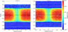 |
Fig. 1 Local CCF map for both nights. Each row corresponds to a local CCF expressed in velocity in the star rest frame at a given time. The two dashed dotted horizontal black lines represent the contact points t1 and t4, the dashed horizontal black lines are t2 and t3, and the vertical dashed black line is at null velocity. The white crosses are the local velocities derived by the Gaussian fit. The RMeffect is clearly visible, as shown by the green trace for both nights. |
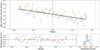 |
Fig. 2 Top: extracted local velocities for both nights (respectively blue and orange for the 2019-02-24 and 2019-03-17) with the best-fit model in black. The vertical dotted lines represent the contact points t1 and t4, the vertical loosely dotted lines represent the contact points t2 and t3, and the vertical dashed line represents mid-transit. Bottom left: local velocity residuals against the best-fit model for both nights. The vertical lines have the same significations as those in the top panel and the horizontal dashed line represents null velocity. Bottom right: distribution of the residuals in the bottom left panel. |
Priors on the stellar rotation model parameters.
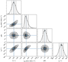 |
Fig. 3 Posterior distribution of the best-fit Rossiter-McLaughlin model done with a Nested sampling and 10 000 living points. |
5 Extraction of planetary atmospheric signal
In this section we describe the reduction steps used to derive the final products: the transmission spectrum and the planetary CCFs. We first corrected for telluric contamination (Sect. 5.1), and then we normalized the spectra (Sect. 5.2) before deriving the transmission spectrum (Sect. 5.3) and the CCFs to search for water vapor (Sect. 5.4).
5.1 Telluric correction
Ground-based spectra are impacted by the Earth’s atmosphere in two different ways. First, the absolute flux is lost, and so calibration is needed to recover it (this is why ground-based transmission spectroscopy is a differential process where in-transit observations are compared to out-of-transit observations). Second, telluric band features absorb the stellar flux at precise wavelengths depending on the species (e.g., H2O, O2, CH4, CO2 or O3). At high resolution, these bands are resolved as a forest of lines. Moreover, emission lines formed at higher altitudes in the Earth’s atmosphere are also spectrally resolved, such as Na, O, and OH. This telluric contamination has a more significant impact at redder wavelengths but strong H2O and O2 bands are already present in the ESPRESSO wavelength range.
We used version 1.5.1 of the Molecfit (Smette et al. 2015; Kausch et al. 2015) software following the method described in (Allart et al. 2017). We adjusted the fit region to the stronger telluric lines that are present in ESPRESSO. To investigate the water residuals, we computed a CCF with a binary telluric mask (see Sects. 5.4 and 6) on the transmission spectrum in the stellar rest frame (which across a night has only a constant shift with respect to the observer rest frame). Due to the higher water vapor content on the first night, a region of 1 Å in width (exclusion of the pixels) around each of the 20 deepest telluric lines has been masked. It is likely that once the telluric lines reach a given depth (70–90%), telluric models are missing some physics that prevents a perfect correction.
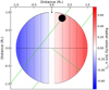 |
Fig. 4 View of the star planet system at the ingress transit. The stellar disk velocity has a color gradient from blue to red representingnegative to positive stellar surface velocity. The stellar rotation axis is shown as the black arrow at the top. The planet is represented by the black disk and occults the red part of the star first and then the blue part, following its misaligned orbit shown in green. The green arrow represents the orbital axis. |
5.2 Normalization
It is necessary to properly normalize the spectra to extract planetary information. Moreover, ESPRESSO spectra are affected by two interference patterns induced by coude train optics. These become apparent when spectra taken in different telescope positions are divided by each other, creating sinusoidal “wiggles”6. The first set of wiggles have a period of 30 Å at 600 nm and an amplitude of ~1% (Tabernero et al. 2020; Borsa et al. 2020; Casasayas-Barris et al. 2020b). In contrast, the second wiggles have a shorter period of 1 Å at 600 nm and an amplitude of ~0.1% (Casasayas-Barris et al. 2020b). Our WASP-127b observations have insufficient S/N to be sensitive to the second wiggles while the first wiggles are detectable and need to be corrected for. In contrast to previous papers (Tabernero et al. 2020; Borsa et al. 2020; Casasayas-Barris et al. 2020b), we decided to correct the wiggles directly on the stellar spectra and not on the transmission spectrum.To do so, we used the publicly available RASSINE code (Cretignier et al. 2020). RASSINE is a python code using an alpha shape strategy (Xu et al. 2019) to normalize the spectrum, taking advantage of nonparametric models to fit the upper envelope of the merged 1d spectrum. The authors showed that alpha shape algorithms could provide more precise and more accurate continuum normalization than classical iterative fitting methods. The only hypothesis behind the algorithm is that the local maxima are probing the continuum of the spectrum.
To fit the wiggles with a periodicity of 30 Å, the alpha shape needs to have a smaller radius in order to capture the modulation. Its value was selected to be about 4 Å here. Appendix E shows the quality of this normalization.
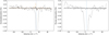 |
Fig. 5 Cross-correlation functions of the transmission spectrum corrected from the telluric features (black) and noncorrected (gray) in the stellar rest frame using the water vapor mask at 296 K for both nights (2019-02-24 and 2019-03-17 from left to right). For the 2019-02-24 night, the dashed orange CCF shows the impact of 20 deepest telluric lines if they are not masked. The blue dashed line shows the observer’s radial velocity, where telluric residuals would be expected. |
5.3 Transmission spectrum
To derive the transmission spectrum, we followed the methods described in Wyttenbach et al. (2015) and Allart et al. (2017), which consist in Doppler shifting the normalized spectrum from the Earth barycentric rest frame to the stellar rest frame by taking into account the systemic velocity and the star radial velocity (from the Keplerian). We then computed the master-out spectrum byaveraging out-of-transit spectra. Individual transmission spectra are obtained by dividing each spectrum by the master-out spectrum. These individual transmission spectra can be used to study the origin of features and their evolution in time (see Sect. 6.2.1). They are then Doppler-shifted to the planet rest frame and averaged. For the atomic species, we applied a weighted average to properly take into account the low core flux of stellar lines. Weights are set to one over the uncertainties squared.
5.4 Cross-correlation function
The CCF is used to maximize the S/N by co-adding hundreds of lines together. In the exoplanets field, two different methods are often used to compute CCFs. The first one is mainly used to derive stellar radial velocities and consists of cross-correlating a spectrum with a binary mask (Baranne et al. 1996; Pepe et al. 2002). This technique is also used for atmospheric characterization (Allart et al. 2017; Pino et al. 2018a, 2020). The second technique consists of cross-correlating a spectrum with a template or model, and is mainly used for atmospheric characterization (Snellen et al. 2010; Birkby et al. 2013; Brogi et al. 2016; Hoeijmakers et al. 2018) but also for stellar radial velocities (Astudillo-Defru et al. 2015; Anglada-Escudé et al. 2016). We discuss the advantages and disadvantages of both methods in more detail in Appendix A. In this paper, we focus on the search for water vapor by applying the binary mask methods to the water band between 7000 and 7500 Å using the HITRAN database (Gordon et al. 2010) for the telluric mask (Sects. 5.1 and 6) and HITEMP for exoplanetary masks (Rothman et al. 2010). We discuss the impact of different line lists in the visible and for our work in Appendix B.
To search for water vapor, we take a step further than Allart et al. (2017), for example, in that we explore the temperature and the number of line parameters in more detail (as discussed in Appendix B). The atmospheric temperature is explored from 100 to 3000 K in steps of 100 K, and the number of lines is explored from 100 to 3000 in steps of 100 lines. We produced CCFs for each set of temperatures and number of lines sampling the velocity space between −50 and 50 km s−1 in steps of 0.5 km s−1, which corresponds to the pixel size. We then fitted a Gaussian on each CCF where the central velocity, the full width at half maximum (FWHM), and amplitudes were respectively initialized to 0 km s−1, 2.5 km s−1, and 100 ppm. We restricted the FWHM to a value above 2 km s−1 in the fit so as to sample at least one ESPRESSO line spread function (LSF). We provide 2D maps (temperature vs. number of lines) reporting the detection level (amplitude divided by its uncertainty), the amplitude, the FWHM, and central velocity. We apply this method to the data in Sect. 6.3 and in Appendix C, where we inject a cloud-free model into the data to validate the procedure.
6 Transmission spectroscopy analysis
In this section, we look at atomic lines such as Na I, K I, Li I, and H-α (Sect. 6.2) that have previously been reported for different exoplanets. We also search for water vapor in Sect. 6.3.
6.1 Telluric contamination
Figure 5 shows the CCF of the transmission spectrum corrected from telluric contamination (black) for both nights obtained with the mask at 296 K (ambient temperature) between 7000 and 7500 Å in the stellar rest frame. The mask is composed of the 150 strongest water telluric lines. If no telluric correction is applied, the corresponding CCFs (in gray) exhibit features at 3 and 5%, respectively. Our telluric correction reduces this feature to the noise level (1-pixel dispersion of 250 and 189 ppm). Nevertheless, some telluric residuals remain for the first night around 0.2% peak-to-valley amplitude over a few pixels despite the telluric masking applied (see Sect. 5.1). However, when we Doppler-shift to the planet rest frame, no residuals impact potential water signatures at null velocity.
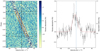 |
Fig. 6 Left: co-addition of the Na doublet lines as a function of orbital phase in the planet rest frame considering the two transits. The vertical black dashed dotted lines represents the expected position of planetary sodium. The two horizontal black dashed lines are the t1 and t4 contact points while the loosely dashed lines are the t2 and t3 contact points. The two orange lines encompass the FWHM of the stellar local lines causing the RM effect. The sodium stellar line core with low S/N is clearly visible in all phases. Right: co-addition of the Na I doublet averaged across the two transitsin gray and binned by ten elements in black. The vertical blue dash dotted line represents the expected position of planetary sodium. The red curve is the best Gaussian fit on the data. |
6.2 Atomic species
For the atomic species, the transmission spectrum was built on each night as the weighted average of the individual transmission spectra. This is done to avoid decreasing the final S/N due to the low flux in the stellar line cores. The RM effect was not corrected for the lines presented hereafter, as it is always encompassed inside the stellar line cores; we verified that excluding these regions when building the transmission spectrum does not change the results. An example of these two effects is presented in Sect. 6.2.1.
6.2.1 The sodium doublet
Figure 6 (left panel) shows the evolution of the co-added sodium doublet lines in velocity space in the planet rest frame. We binned the two transits on this map. One can see the individual transmission spectra for each night at the lower and higher phases where the two datasets do not overlap. The low S/N of the stellar sodium line cores is also clearly visible as a noisy band showing both excess emission (blue) and excess absorption (orange) following the stellar track (Borsa & Zannoni 2018). Such an effect cannot be mistaken for any other as it is high-frequency noise that is present not only during transit but at all phases. The expected impact of the RM effect is encompassed by the white lines that follow the local stellar velocity in the rest frame of the planet. Moreover, due to the slow change of stellar velocity across the transit chord, the RM effect is only present inside the low-S/N regions of the stellar sodium line cores, as discussed previously. In addition, one can also see some broad excess absorption following the sodium planetary track in blue. Figure 6 (right panel) shows the transmission spectrum of the co-added sodium lines in the planet rest frame. Excess absorption is visible and Gaussian fits yield an excess absorption of 0.34 ± 0.04% (9-σ) with a blueshift of 2.74 ± 0.79 km s−1 and a FWHM of 15.18 ± 1.75 km s−1. This excess absorption corresponds to an extension of the atmosphere of 1.15 Rp (6.8 scale heights), which is well below the Roche Lobe radius (1.96 Rp).
To validate the significance of this signal, we performed empirical Monte Carlo (EMC) simulations. We followed the method described in Wyttenbach et al. (2015), Casasayas-Barris et al. (2019) and Seidel et al. (2019), which consists of generating three scenarios (in/in, out/out, and in/out) of 10 000 iterations each. For one iteration, the in- and out-of-transit spectra are randomized among the pool of spectra for the considered scenario. The absorption was measured on a 2 Å passband centered on both lines on the transmission spectrum. The results are shown in Fig. 7. As expected, the in/in and out/out scenarios are centered at zero absorption while the in/out scenario shows excess absorption. These EMC simulations confirm that the absorption signal is not serendipitous but is linked to the planet atmosphere.
As the co-addition of the two sodium lines has a detected planetary signal, we analyze the individual lines in Fig. 8 for Na I D1 and Na I D2. These two lines are compatible with excess absorption of 0.26 ± 0.05% and 0.36 ± 0.06%, a radial velocity shift of 1.19 ± 1.60 km s−1 and −2.02 ± 1.31 km s−1, and a FWHM of 20.43 ± 3.46 km s−1 and 18.70 ± 2.80 km s−1, respectively.
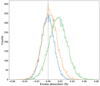 |
Fig. 7 Empirical Monte Carlo simulations for the co-addition of the sodium doublet. Three distributions have been randomized 10 000 times each: the in/in distribution (blue), the out/out distribution (orange), and the in/out distribution (green). As expected, only the in/out distribution exhibits excess absorption. |
6.2.2 Other atmospheric tracers: K, Li, and H-α
We also searched for the potassium D1 line at 7698.96 Å (the K I D2 line was not studied due to strong O2 telluric contamination), the lithium line at 6707.76 Å, and the H-α line at 6562.82 Å. Similarly to the Na I doublet, these lines are affected by low S/N residuals in the stellar line core. In Figs. 9–11, we present the combined transmission spectrum around each line. However, we do not detect any of the species even if the 1-pixel dispersion is respectively of 0.14, 0.12, and 0.20%. Assuming a line width of 10 km s−1 and following the formalism of Allart et al. (2017), we can exclude excess absorption from these atmospheric tracers at a confidence level of 0.09, 0.08, and 0.13% at 3-σ. These upper limits correspond to 1.04, 1.04, and 1.06 Rp or 1.9, 1.7, and 2.8 scale height (H).
6.3 Search for water vapor
We applied the method described in Sect. 5.4, and show in Fig. 12 the detection levels obtained from a Gaussian fit applied to the set of CCFs spanning temperatures from 100 to 3000 K and including from 100 to 3000 lines. All CCFs have Gaussian features with a confidence level of 3.6-σ at most. Wetherefore conclude that there is no robust detection of water vapor at visible wavelengths.
To constrain the presence of water vapor and based on the equilibrium temperature and the results of Appendix C, we looked at the CCF built with the mask with 1400 K and 1600 lines. This is shown in Fig. 13 for both nights and the average.We added the CCF from Fig. 12 for comparison, showing the highest confidence level obtained with the mask at 600 K and 1900 lines. The lack of difference between both CCFs reinforce the claim of nondetection.
The one-pixel dispersion in the continuum for both nights is of 41 and 57 ppm, respectively, for the CCF at 1400 K and 1600 lines, and of 29 ppm for the combined CCF. Based on Appendix C, we can assume a line width of 2.5 km s−1 leading to a 1-σ precision of 13 ppm and thus to a 3-σ upper limit of 38 ppm which corresponds to 0.08 H. We describe the impact of this extreme precision in Sect. 7.
Atmospheric detection and nondetection summary for WASP-127b with ESPRESSO.
7 Combining low- and high-resolution spectroscopy
Table 4 summarizes the detection and nondetection obtained with the ESPRESSO data. In this section, we first reconciliate the low-resolution HST results with our high-resolution results and then discuss the sodium detection in more detail.
ESPRESSO allows us to reach a fine 1-σ precision of 13 ppm in our search for water vapor in the visible wavelengths, which translates into a 3-σ upper limit of 0.08 H. This unique precision can be used to largely constrain the presence of clouds in the atmosphere of exoplanets by studying several water bands (Pino et al. 2018a; Alonso-Floriano et al. 2019; Sánchez-López et al. 2019). Therefore, to see if the water detection at 1.3 microns obtained at low-resolution is compatible with the nondetection obtained in the visible at high-resolution, we computed a set of high-resolution models described in Sect. 7.1 to match both results.
7.1 Model description
To interpret our results we employed the πη line-by-line radiative transfer code (Ehrenreich et al. 2006, 2012; Pino et al. 2018b). This code was already applied for the simultaneous interpretation of ground-based, optical, high-spectral-resolution observations with HARPS and HST/WFC3observations (Pino et al. 2018a). Here, we employ the version by Pino et al. (2018a), who extended π η to simulate thewater bands observed by multiple optical to NIR high-spectral-resolution instruments including ESPRESSO, and which is therefore suitable for our requirements.
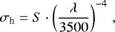
The considered opacity sources include sodium, potassium, water, Rayleigh scattering by molecular hydrogen, collisional-induced absorption (CIA), and aerosols distinguished between a gray absorber and a chromatic absorber. We name these latter “clouds” and “hazes” respectively, following the convention by Earth atmosphere scientists. The alkali doublets are modeled with a Voigt profile following Burrows et al. (2000) and Iro et al. (2005). For water, we employ the HITEMP line list (Rothman et al. 2013), converted to a cross-section with the HELIOS-K code (Grimm & Heng 2015). The Rayleigh scattering cross-section for molecular hydrogen follows Dalgarno & Williams (1962, 1965), and the CIA cross-section follows Richard et al. (2012). Gray aerosols are modeled by setting the atmosphere as opaque below a pressure Pc. Finally, the cross-section of chromatic absorption by aerosols (σh) is modeled as a power law of the form:
 (1)
(1)
where λ is the wavelength in Angstroms and S is a scale factor normalized to the Rayleigh scattering cross-section of molecular hydrogen at 3500 Å. Gray absorbers dominate the aerosol opacity budget at the wavelengths of our interest covered by ESPRESSO and HST WFC3, and therefore we consider our simple model to be adequate for our purposes. Pino et al. (2018b) provide a detailed description of the opacities and the assumptions in the model.
A full joint low-resolution (LR) + high-resolution (HR) retrieval is beyond the scope of this paper. We instead consider an isothermal atmosphere, fix the abundances of sodium, potassium, and water to the free-free retrieval results by Spake et al. (2020), and produce a grid of models with different cloud coverage. Indeed, for a given abundance and reference pressure and radius, it is aerosol coverage that controls the relative strength of water features (de Kok et al. 2014; Pino et al. 2018a), which is our observable at high spectral resolution. Table 5 summarizes the parameters employed in our grid of models.
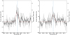 |
Fig. 8 Transmission spectrum around the Na D2 (left) and Na D1 (right) line averaged across the two transits in gray and binned by fifteen elements in black. The vertical blue dash dotted line represents the expected position of planetary sodium lines. |
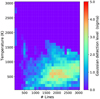 |
Fig. 12 Detectability map based on a Gaussian fit for a set of binary CCFs with temperature ranging from 100 to 3000 K and including from the 100 to 3000 strongest water lines. |
7.2 Water vapor and cloud-deck
We first convolved the models to the HST resolution and binned the models to match the Spake et al. (2020) data sampling. We then adjusted each LR model to these data by fitting a constant vertical offset. The  and BIC values are reported in Table 6. Figures 14 and 15 show these latter models and the HST data.
Concomitantly, we convolved the high-resolution model (HR model) by the instrumental LSF (2.0 km s−1) of ESPRESSO and the planetary rotation (1.7 km s−1 assuming tidal-lock rotation). We resampled the HR models to match the ESPRESSO sampling. We then only consider the spectral range between 6250 and 7600 Å for which we removed the continuum to render the HR models as they should be observed from the ground, where the continuum is lost. Those excess absorption HR models are shown in the middle column of Fig. 15. Hereafter, we injected those HR models into the ESPRESSO data, and we computed the CCFs with a binary mask at Teq and 1600 lines. Finally, we fitted a Gaussian to each of those CCFs to measure whether or not the injected signal can be retrieved. Table 6 provides the Gaussian amplitude and the detection level.
Based on this analysis, which is summarized in Fig. 15 and Table 6, we can see not only whether or not one model can reproduce both LR infrared and HR visible result but also what constraint the ESPRESSO data can bring to HST/WFC3 data. On the LR side, we see that the cloud-free (Pc > 100 mbar) and the most cloudy models do not show a close fit to the HST/WFC3 data, but that in between there are a range of models that do. The best model is obtained for pressure of 0.5 mbar, but models with pressure ranging from 0.3 to 1 mbar are equally good as their ΔBIC is lower than 6. On the HR side, we can see that a clear signal is detected for the cloud-free models (see as expected in Appendix C), and therefore those models do not reproduce the ESPRESSO results (Sect. 6.3). Models for which the injected signal is recovered at more than 3-σ (i.e., a hint of detection) can be rejected. Therefore, our ESPRESSO data are compatible with gray clouds that have a pressure below 0.5 mbar. Combining the LR and HR data allows us to constrain the cloud-deck pressure between 0.3 and 0.5 mbar. Based on the best model (P = 0.3 mbar), we estimate that the 1.3 μm water band at high-resolution extend up to 6 scale heights. This is the first time that high-resolution visible data are used to constrain the presence of clouds using water vapor lines. It is important to remember that there is a degeneracy with water abundance and reference pressure, and that we chose only the best fit values from Spake et al. (2020).
7.3 Atomic species
High-resolution data from the ground cannot probe the wings of the line far from the core because of the loss of absolute flux level. However, for low-resolution spectrographs, the line cores are diluted over tens of angstroms. The lack of line-core signal can be compatible with the presence of wings if processes such as ionization are considered. The ESPRESSO data do not indicate the presence of potassium or lithium cores with an upper limit of 1.9 and 1.7 H. Potassium and lithium have only been reported on one LR dataset (Chen et al. 2018) but not with HST (Spake et al. 2020). Therefore, the situation is currently unclear with respect to potassium and lithium in the atmosphere of WASP-127b.
As presented in Sect. 6.2.1, we report the detection of sodium in the atmosphere of WASP-127b at the 9-σ level. We compare its absorption with LR datasets by convolving our transmission spectrum around sodium to the resolution of HST/STIS and by binning over 35 Å to fit the HST/STIS bin centered at 5895 Å. Our ESPRESSO Na excess absorption of ~0.34% becomes an excess absorption of ~0.03% over the 35 Å bin, which is consistent with the relative absorption between the HST bin centered at 5895 Å and its two adjacent bins. Therefore, our high-resolution detection is compatible with the detection of Spake et al. (2020), and also with that of Chen et al. (2018) who detected similar signal to that detected by HST.
We also report a slight blueshift on the sodium core of 2.74 ± 0.79 km s−1. Blueshifts are not unusual for lukewarm and hot gas-giant exoplanets, with several such reports (Snellen et al. 2010; Wyttenbach et al. 2015; Louden & Wheatley 2015; Brogi et al. 2016; Allart et al. 2018; Hoeijmakers et al. 2018; Flowers et al. 2019; Bourrier et al. 2020; Ehrenreich et al. 2020) and could be due to zonal winds from the day-to-night side. In the inset of Fig. 14, we overplot the high-resolution model normalized to the local continuum on our Na detection. As we are looking at the very narrow core of the planetary lines, the pressure cut applied does not impact the doublet line depth and all our models are thus similar. While our model reproduces the HST/STIS data as we assumed the same Na abundance as Spake et al. (2020), the shape is different at high resolution. Our model has an expected Na signature of about 1% which does not accurately reproduce the observed excess absorption. This difference might be due to a lack of hazes or an inappropriate Na abundance in our model. Moreover, the FWHM is not compatible either and is degenerate with many parameters such as Na abundance, hazes, various wind patterns, and thermal broadening (e.g., Seidel et al. 2020b; Wyttenbach et al. 2020). In order to explain how such a small extension is possible, a dedicated modeling of this signature is needed.
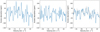 |
Fig. 13 Measured CCFs in the planet rest frame with water vapor mask at 1400 K and 1600 lines for both nights (left panel: 2019-02-24 and middle panel: 2019-03-17) and the combination of them (right panel). Right panel: combined CCF with the highest confidence level from the map of temperature vs. number lines (600 K and 1900 lines; Fig. 12) has been added in gray. |
Input πη parameters used in our model grid.
Gray cloud exploration through injection tests to combine low- and high-resolution datasets.
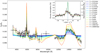 |
Fig. 14 Low-resolution model described in Sect. 7.1 with different cut in pressure to represent various gray cloud-decks (colored curves). In black, the HST data from Spake et al. (2020). The inset is the same as in Fig. 6 (right panel) where we added the high-resolution model Na doublet lines (green) which are not affected by the cloud-deck pressure. |
8 Conclusion
We analyzed two transits of WASP-127b observed with ESPRESSO. We detected an RM effect for this object for the first time and concluded that the planet has a misaligned retrograde orbit. We searched for the presence of atomic species, and despite the extreme precision of a few scale heights, we did not detect K, Li, or H-α. Nonetheless, we confirm the presence of sodium by measuring an excess absorption arising from the Na doublet core lines, which extends up to 7 H only. This Na detection is compatible with those reported in the literature at low resolution (Chen et al. 2018; Spake et al. 2020). In comparison, the water band at 1.3 μm extends up to 6 H if seen at high-resolution. Therefore, Na and H2O are probing the same atmospheric layers which is relatively uncommon for gas-giant planets.
We propose a new framework to search for water vapor and other molecular species at high resolution. This framework is based on Occam’s razor principle to minimize the model-dependent variables. We tested it with success by injecting a model into the data, and then we applied it to the ESPRESSO data. Unfortunately, despite the good data quality, we did not detect water vapor, but we fixed an upper limit of 38 ppm on the presence of water in the 700–750 nm passband. Finally, we combined this result with a low-resolution detection of water at 1.3 μm to constrain the presence of clouds in the atmosphere of WASP-127b.
In summary, we report for the first time that high-resolution visible data can be used to differentiate between cloudy and cloud-free exoplanets by measuring the water content and can also provide essential information on the cloud-deck pressure. The framework developed here to measure this water content will be applied to other exoplanets in the ESPRESSO GTO atmospheric survey and to other surveys such as the NIRPS GTO atmospheric survey. One of the primary targets for this latter survey could indeed be WASP-127b, where the NIR water excess absorption would be about 800–1000 ppm once the telluric saturation bands are excluded.
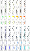 |
Fig. 15 Combining low- and high-resolution datasets. The color-code is the same as in Fig. 14. Left column: ESPRESSO CCFs with injected models retrieved for the equilibrium temperature and 1600 lines. The best Gaussian-fit model shown in black evaluates whether or not the injected model could be retrieved in the ESPRESSOdata. Middle column: high-resolution model that is injected into the ESPRESSO data. Right column: HST data in black are compared to low-resolution models. A minimization algorithm is applied to estimate the
|

Acknowledgements
We thank the referee for their careful reading and their inputs. The authors acknowledge the ESPRESSO project team for its effort and dedication in building the ESPRESSO instrument. We thank Jessica Spake for the discussion on the HST datasets and important insight. We thank Monika Lendl and Julia Seidel for their important feedback and discussions on the EulerCam and HARPS data. We acknowledge the Geneva exoplanet atmosphere group for fruitful discussions. This work has been carried out within the frame of the National Centre for Competence in Research’ PlanetS’ supported by the Swiss National Science Foundation (SNSF). The authors acknowledge the financial support of the SNSF. The research leading to these results has received funding from the European Research Council (ERC) under the European Union’s Horizon 2020 research and innovation programme (grant agreement No. 679633: Exo-Atmos). This work was supported by FCT – Fundação para a Ciência e a Tecnologia through national funds and by FEDER through COMPETE2020 – Programa Operacional Competitividade e Internacionalização by these grants: UID/FIS/04434/2019; UIDB/04434/2020; UIDP/04434/2020; PTDC/FIS-AST/32113/2017 & POCI-01-0145-FEDER-032113; PTDC/FIS-AST/28953/2017 & POCI-01-0145-FEDER-028953; PTDC/FIS-AST/28987/2017 & POCI-01-0145-FEDER-028987 & PTDC/FIS-OUT/29048/2017 & IF/00852/2015. This project has received funding from the European Research Council (ERC) under the European Union’s Horizon 2020 research and innovation programme (project Four Aces grant agreement No 724427). O.D.S.D. is supported by by national funds through Fundação para a Ciência e Tecnologia (FCT) in the form of a work contract (DL 57/2016/CP1364/CT0004) and project related funds (EPIC: PTDC/FIS-AST/28953/2017 & POCI-01-0145-FEDER-028953). The INAF authors acknowledge financial support of the Italian Ministry of Education, University, and Research with PRIN 201278X4FL and the “Progetti Premiali” funding scheme. V.A. acknowledges the support from FCT through Investigador FCT contract nr. IF/00650/2015/CP1273/CT0001. This work has made use ofdata from the European Space Agency (ESA) mission Gaia (https://www.cosmos.esa.int/gaia), processed by the Gaia Data Processing and Analysis Consortium (DPAC, https://www.cosmos. esa.int/web/gaia/dpac/consortium). Funding for the DPAC has been provided by national institutions, in particular the institutions participating in the Gaia Multilateral Agreement.
Appendix A Binary masks or template matching for CCFs
In this appendix, we describe the main difference between a CCF obtained through cross-correlation with a model or with a binary mask for atmospheric characterization. Both methods rely on different assumptions, which are discussed below, but they both require a line list. The line-list selection is discussed in Appendix B. Nonetheless, the main idea is similar and consists of co-adding hundreds of lines to create an average line. Molecular lines in a planetary spectrum have different depths, and when hundreds of them are combined, the weakest lines will decrease the S/N. Therefore, it is important to give proper weight to each line to maximize the S/N.
A.1 Template matching
Template matching is the most commonly used technique to detect molecular species in exoplanet atmospheres (e.g., Snellen et al. 2010; Birkby et al. 2013; Brogi et al. 2016). It consists in building an atmospheric model that depends on the line positions, line cross-sections, temperature, mean-molecular weight, molecule abundance, cloud-deck, and haze scattering. The model produced therefore has a proper weight of the intrinsic depth of the lines at each pixel. However, this technique requires prior knowledge of the atmospheric properties or accurate estimates. Hence, a grid of models is required, which is computationally heavy. Recently, Brogi & Line (2019) and Gibson et al. (2020) proposed and tested Bayesian frameworks to find the model that best maximizes the S/N. These frameworks are able to retrieve abundances and reconstruct the temperature-pressure profile, and can be used on low- and high-resolution datasets simultaneously. Finally, this method does not allow the user to easily retrieve basic properties (it requires the new Bayesian framework) of the average line such as its amplitude, its FWHM, or the continuum dispersion that can be useful to compare to other results directly.
A.2 Binary masks
This method for atmospheric studies has barely been used so far (Allart et al. 2017; Pino et al. 2018a, 2020). It consists of building a binary mask (with an aperture width of one pixel) and summing the transmitted flux at each wavelength. The mask apertures are centered on the theoretical line positions, which depend only on the temperature and are associated with a given weight. Accordingly, this technique relies on three parameters: line positions, temperature, and weights, and is not defined over the full spectral range. The major and more problematic question linked to this method is how the weights have to be set. In contrast with stellar masks used to extract radial velocities, it is not possible to measure the line contrasts for a given planet and apply them to all exoplanets. The weights of exoplanet masks encompass all the other parameters described in Appendix A.1. Hoeijmakers et al. (2019) used a mixed approach between template matching and binary mask, which consists in using designed templates for a given planet to set the weights. Here, we fixed the weight to one for each line to minimize model assumptions and follow Occam’s razor principle. Now the difficulty lies in how many lines have to be included in the mask starting from the strongest to maximize the S/N. On the one hand, including only a handful of lines maximizes the CCF signal, as well as the noise. On the other hand, including all the lines minimizes the noise but at the expense of removing the signaldue to the thousands of weak lines. To maximize the S/N, it is therefore necessary to optimize the number of lines in the mask, but this number cannot be known a priori. While the template matching requires several parameters, the technique proposed here relies only on two parameters (temperature and number of lines), which can be explored relatively quickly. Moreover, the produced average line can be expressed in terms of its basic properties.
A.3 Complementarity between both methods
The two methods are indeed complementary and can be used in a two-step approach. First, the binary mask method is applied – as it is faster – to retrieve the basic properties of the average line and give a first constraint on the temperature range. The template matching method then comes in a second step to retrieve the atmospheric properties in greater detail (e.g., temperature-pressure profile, abundances, cloud-deck). We also note that in Pino et al. (2020), the authors proposed a binary mask Bayesian framework, benchmarked it with template matching Bayesian framework (Brogi & Line 2019), and retrieved detailed information on the atmosphere of KELT-9b.
Appendix B Line-list comparison for water at visible wavelengths
Various molecular line lists (e.g., HITEMP, ExoMol,...) can reproduce broad-band detection as in the 1.3 micron water band. However, toward higher resolutions where individual lines are resolved ( 100 000), the line positions and cross-sections are less reliable7. Gandhi et al. (2020) studied the impact of different line lists in the infrared. The authors showed that water line lists mostly diverge for temperatures above 1200 K and for low-opacity lines. On the contrary, the strongest water lines are in agreement between line lists in terms of position and intensity. Here, we focus on the search for water vapor in the visible range (7000–7500 Å) and we compare three existing line lists: ExoMol BT2 (Barber et al. 2006), Exomol Pokazatel (Polyansky et al. 2018), and HITEMP2010 (Rothman et al. 2010). We applied the same technique as described in Sect. 5.4 for each line list. Figure B.1 shows the CCFs for a temperature of 1400 K and 1600 lines for each line list, clearly revealing that the three line lists present the same broad patterns, but none of them show a water signature. There are two possible explanations for this: either the water signal is muted by the cloud-deck, as we propose, or all line lists are equally poor in the visible and thus prevent a search for water vapor.
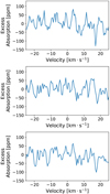 |
Fig. B.1 Cross correlation functions for the ExoMol BT2 (top panel), the ExoMol Pokazatel (middle panel), and the HITEMP2010 (bottom panel) with a water binary mask at 1400 K and 1600 lines. |
Appendix C Injection model and constraints from binary masks
In this appendix, we inject the cloud-free model described in Sect. 7.1 to see if our reduction steps described in Sect. 5 can modify or erase a planetary signature. Our second goal is to apply our CCF binary mask framework to the ESPRESSO data when a planetary signature is present. To this aim, we injected the cloud-free model to each in-transit spectrum before applying the telluric correction. We then reran the Molecfit correction and the RASSINE normalization before extracting the transmission spectrum and deriving the CCFs.
Figure C.1 presents the map of temperature versus number lines described in Sect. 5.4 and reports the best value for each parameter of the Gaussian fit applied to each CCF. First, the detection map (top row) shows clearly that the injected water vapor signature is detected and that the binary mask procedure allows to us constrain the water vapor temperature and additionally,the weights of the lines (expressed as the number of strongest lines). Second, while the Gaussian amplitude varies as expected (strongest amplitudes when fewer lines are included in the mask), it does not provide a strong constraint on the signal apart from an indicative mean amplitude of the water lines. Finally, the Gaussian FWHM and centroid are used to verify that the detection is not obtained for low or high-frequency noise at a velocity far from 0 km s−1.
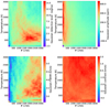 |
Fig. C.1 Map of temperature vs. number of lines representing the Gaussian fit outputs for each CCF set. From top to bottom: detection level, amplitude, FWHM, and centroid position. |
Figure C.2 shows the observed CCF that maximizes the detection for the equilibrium temperature, and the model CCF using the same mask. One can see that the injected signal is well detected, and it is also recovered in the 1-σ uncertainty. Therefore, our reduction steps, including telluric correction, normalization, wiggle removal, and interpolation due to Doppler-shifts, do not modify or erase a planetary signature.
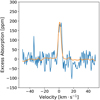 |
Fig. C.2 Measured CCF with the injected model with the water vapor mask at 1400 K and 1600 lines in blue. The same mask is used to compute the modeled CCF shown in orange. This mask is used as it maximizes the detection level with the temperature fixed to Teq. |
As a general comment, the decision to look at the CCFs at Teq and not at the HST/WFC3 retrieval temperature used to compute the model can be explained in two points. Firstly, we want to follow a model-independent approach as much as possible, which favors choosing the equilibrium temperature and not the one from a retrieval. Secondly, MacDonald et al. (2020) discuss in great detail why HST/WFC3 retrievals applied to the water band at 1.3 μm found temperatures lower than the equilibrium temperatures. The explanation is based on the lack of sophistication of those models which are generally 1D and do not allow different compositions between terminators, thus leading to erroneous abundance, temperature, and temperature gradient.
Appendix D Radial velocities
In this appendix, we show the radial velocities of WASP-127b phase-folded around mid-transit to illustrate the classical Rossiter-Mclaughlin effect. We can clearly see the RM effect expected for a retrograde orbit with negative velocities during the first part of the transit followed by positive radial velocities.
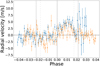 |
Fig. D.1 Radial velocities of WASP-127b for both transits (respectively blue and orange for the 2019-02-24 and 2019-03-17) phased-folded. The radial velocities have been corrected from the vsyst and the Keplerian model. The vertical dashed line is the mid-transit while the dense vertical dotted lines correspond to t1 and t4 and the vertical dotted lines are t2 and t3. The horizontal dashed line corresponds to null velocity. |
Appendix E Impact of the normalization
In this appendix, we show the impact of the RASSINE (Cretignier et al. 2020) normalization on the transmission spectrum. The wiggles are well suppressed by the RASSINE normalization but a few residuals are still present. This is due to the choice of the preliminary mode of spectra time-series normalization of RASSINE rather than the complete version because this latter could absorb true planetary signatures in the Savitchy-Golay filtering. This was discussed by Cretignier et al. (2020) in Fig. 4 of their paper.
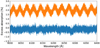 |
Fig. E.1 Transmission spectrum with (blue) or without (orange) the RASSINE normalization for the 2019-02-24 transit. |
References
- Albrecht, S., Winn, J. N., Johnson, J. A., et al. 2012, ApJ, 757, 18 [NASA ADS] [CrossRef] [Google Scholar]
- Allart, R., Lovis, C., Pino, L., et al. 2017, A&A, 606, A144 [NASA ADS] [CrossRef] [EDP Sciences] [Google Scholar]
- Allart, R., Bourrier, V., Lovis, C., et al. 2018, Science, 362, 1384 [Google Scholar]
- Allart, R., Bourrier, V., Lovis, C., et al. 2019, A&A, 623, A58 [NASA ADS] [CrossRef] [EDP Sciences] [Google Scholar]
- Alonso-Floriano, F. J., Sánchez-López, A., Snellen, I. A. G., et al. 2019, A&A, 621, A74 [NASA ADS] [CrossRef] [EDP Sciences] [Google Scholar]
- Anglada-Escudé, G., Amado, P. J., Barnes, J., et al. 2016, Nature, 536, 437 [NASA ADS] [CrossRef] [PubMed] [Google Scholar]
- Astudillo-Defru, N., Bonfils, X., Delfosse, X., et al. 2015, A&A, 575, A119 [NASA ADS] [CrossRef] [EDP Sciences] [Google Scholar]
- Baranne, A., Queloz, D., Mayor, M., et al. 1996, A&AS, 119, 373 [NASA ADS] [CrossRef] [EDP Sciences] [Google Scholar]
- Barber, R. J., Tennyson, J., Harris, G. J., & Tolchenov, R. N. 2006, MNRAS, 368, 1087 [NASA ADS] [CrossRef] [Google Scholar]
- Batygin, K., Stevenson, D. J., & Bodenheimer, P. H. 2011, ApJ, 738, 1 [NASA ADS] [CrossRef] [Google Scholar]
- Birkby, J. L., de Kok, R. J., Brogi, M., et al. 2013, MNRAS, 436, L35 [NASA ADS] [CrossRef] [Google Scholar]
- Bodenheimer, P., Lin, D. N. C., & Mardling, R. A. 2001, ApJ, 548, 466 [NASA ADS] [CrossRef] [Google Scholar]
- Bodenheimer, P., Laughlin, G., & Lin, D. N. C. 2003, ApJ, 592, 555 [NASA ADS] [CrossRef] [Google Scholar]
- Borsa, F., & Zannoni, A. 2018, A&A, 617, A134 [NASA ADS] [CrossRef] [EDP Sciences] [Google Scholar]
- Borsa, F., Rainer, M., Bonomo, A. S., et al. 2019, A&A, 631, A34 [NASA ADS] [CrossRef] [EDP Sciences] [Google Scholar]
- Borsa, F., Allart, R., Casasayas-Barris, N., et al. 2020, A&A, in press, https://doi.org/10.1051/0004-6361/202039344 [Google Scholar]
- Borucki, W. J., Koch, D. G., Lissauer, J. J., et al. 2003, SPIE Proc. Ser., 4854, 129 [NASA ADS] [CrossRef] [Google Scholar]
- Bourrier, V., Cegla, H. M., Lovis, C., & Wyttenbach, A. 2017, A&A, 599, A33 [NASA ADS] [CrossRef] [EDP Sciences] [Google Scholar]
- Bourrier, V., Lovis, C., Beust, H., et al. 2018, Nature, 553, 477 [NASA ADS] [CrossRef] [Google Scholar]
- Bourrier, V., Ehrenreich, D., Lendl, M., et al. 2020, A&A, 635, A205 [NASA ADS] [CrossRef] [EDP Sciences] [Google Scholar]
- Bressan, A., Marigo, P., Girardi, L., et al. 2012, MNRAS, 427, 127 [NASA ADS] [CrossRef] [Google Scholar]
- Brogi, M., & Line, M. R. 2019, AJ, 157, 114 [NASA ADS] [CrossRef] [Google Scholar]
- Brogi, M., de Kok, R. J., Albrecht, S., et al. 2016, ApJ, 817, 106 [Google Scholar]
- Brown, D. J. A., Triaud, A. H. M. J., Doyle, A. P., et al. 2017, MNRAS, 464, 810 [Google Scholar]
- Buchner, J., Georgakakis, A., Nandra, K., et al. 2014, A&A, 564, A125 [NASA ADS] [CrossRef] [EDP Sciences] [Google Scholar]
- Burrows, A., Marley, M. S., & Sharp, C. M. 2000, ApJ, 531, 438 [NASA ADS] [CrossRef] [Google Scholar]
- Casasayas-Barris, N., Pallé, E., Yan, F., et al. 2019, A&A, 628, A9 [NASA ADS] [CrossRef] [EDP Sciences] [Google Scholar]
- Casasayas-Barris, N., Pallé, E., Yan, F., et al. 2020a, A&A, 635, A206 [NASA ADS] [CrossRef] [EDP Sciences] [Google Scholar]
- Casasayas-Barris, N., Pallé, E., Stangret, M., et al. 2020b, A&A, submitted [Google Scholar]
- Cegla, H. M., Lovis, C., Bourrier, V., et al. 2016, A&A, 588, A127 [NASA ADS] [CrossRef] [EDP Sciences] [Google Scholar]
- Chen, G., Pallé, E., Welbanks, L., et al. 2018, A&A, 616, A145 [NASA ADS] [CrossRef] [EDP Sciences] [Google Scholar]
- Cosentino, R., Lovis, C., Pepe, F., et al. 2012, SPIE, 8446, 84461V [Google Scholar]
- Cretignier, M., Francfort, J., Dumusque, X., Allart, R., & Pepe, F. 2020, A&A, 640, A42 [CrossRef] [EDP Sciences] [Google Scholar]
- Dalgarno, A., & Williams, D. A. 1962, ApJ, 136, 690 [NASA ADS] [CrossRef] [Google Scholar]
- Dalgarno, A., & Williams, D. A. 1965, Planets Planet System, 85, 685 [Google Scholar]
- da Silva, L., Girardi, L., Pasquini, L., et al. 2006, A&A, 458, 609 [NASA ADS] [CrossRef] [EDP Sciences] [Google Scholar]
- de Kok, R. J., Birkby, J., Brogi, M., et al. 2014, A&A, 561, A150 [NASA ADS] [CrossRef] [EDP Sciences] [Google Scholar]
- Deming, D., Wilkins, A., McCullough, P., et al. 2013, ApJ, 774, 95 [Google Scholar]
- dos Santos, L. A., Ehrenreich, D., Bourrier, V., et al. 2020, A&A, 640, A29 [CrossRef] [EDP Sciences] [Google Scholar]
- Ehrenreich, D., Tinetti, G., Lecavelier Des Etangs, A., Vidal-Madjar, A., & Selsis, F. 2006, A&A, 448, 379 [NASA ADS] [CrossRef] [EDP Sciences] [Google Scholar]
- Ehrenreich, D., Vidal-Madjar, A., Widemann, T., et al. 2012, A&A, 537, L2 [NASA ADS] [CrossRef] [EDP Sciences] [Google Scholar]
- Ehrenreich, D., Lovis, C., Allart, R., et al. 2020, Nature, 580, 597 [Google Scholar]
- Fabrycky, D., & Tremaine, S. 2007, ApJ, 669, 1298 [NASA ADS] [CrossRef] [Google Scholar]
- Feroz, F., & Hobson, M. P. 2008, MNRAS, 384, 449 [NASA ADS] [CrossRef] [Google Scholar]
- Feroz, F., & Skilling, J. 2013, Bayesian Inference and Maximum Entropy Methods in Science and Engineering: 32nd International Workshop on Bayesian Inference and Maximum Entropy Methods in Science and Engineering Place, 1553, 106 [Google Scholar]
- Feroz, F., Hobson, M. P., & Bridges, M. 2009, MNRAS, 398, 1601 [NASA ADS] [CrossRef] [Google Scholar]
- Flowers, E., Brogi, M., Rauscher, E., Kempton, E. M.-R., & Chiavassa, A. 2019, AJ, 157, 209 [NASA ADS] [CrossRef] [Google Scholar]
- Gaia Collaboration 2018, VizieR Online Data Catalog: I/345 [Google Scholar]
- Gandhi, S., Brogi, M., Yurchenko, S. N., et al. 2020, MNRAS, 495, 224 [CrossRef] [Google Scholar]
- Gibson, N. P., Merritt, S., Nugroho, S. K., et al. 2020, MNRAS, 493, 2215 [Google Scholar]
- Gordon, I. E., Rothman, L. S., Hill, C., et al. 2010, J. Quant. Spectr. Rad. Transf., 111, 2139 [NASA ADS] [CrossRef] [Google Scholar]
- Grimm, S. L.,& Heng, K. 2015, ApJ, 808, 182 [NASA ADS] [CrossRef] [Google Scholar]
- Hoeijmakers, H. J., Ehrenreich, D., Heng, K., et al. 2018, Nature, 560, 453 [NASA ADS] [CrossRef] [Google Scholar]
- Hoeijmakers, H. J., Ehrenreich, D., Kitzmann, D., et al. 2019, A&A, 627, A165 [NASA ADS] [CrossRef] [EDP Sciences] [Google Scholar]
- Iro, N., Bézard, B., & Guillot, T. 2005, A&A, 436, 719 [NASA ADS] [CrossRef] [EDP Sciences] [Google Scholar]
- Kausch, W., Noll, S., Smette, A., et al. 2015, A&A, 576, A78 [NASA ADS] [CrossRef] [EDP Sciences] [Google Scholar]
- Kozai, Y. 1962, AJ, 67, 591 [Google Scholar]
- Kreidberg, L. 2015, PASP, 127, 1161 [NASA ADS] [CrossRef] [Google Scholar]
- Kreidberg, L., Bean, J. L., Désert, J.-M., et al. 2014, Nature, 505, 69 [NASA ADS] [CrossRef] [Google Scholar]
- Kurucz, R. L. 1993, Kurucz CD-ROM (Cambridge, MA: Smithsonian Astrophysical Observatory) [Google Scholar]
- Lam, K. W. F., Faedi, F., Brown, D. J. A., et al. 2017, A&A, 599, A3 [NASA ADS] [CrossRef] [EDP Sciences] [Google Scholar]
- Lavie, B., Mendonça, J. M., Mordasini, C., et al. 2017, AJ, 154, 91 [NASA ADS] [CrossRef] [Google Scholar]
- Lecavelier Des Etangs, A. 2007, A&A, 461, 1185 [NASA ADS] [CrossRef] [EDP Sciences] [Google Scholar]
- Lopez, E. D., & Fortney, J. J. 2016, ApJ, 818, 4 [NASA ADS] [CrossRef] [Google Scholar]
- Louden, T., & Wheatley, P. J. 2015, ApJ, 814, L24 [NASA ADS] [CrossRef] [Google Scholar]
- MacDonald, R. J., Goyal, J. M., & Lewis, N. K. 2020, ApJ, 893, L43 [CrossRef] [Google Scholar]
- Mayor, M., Pepe, F., Queloz, D., et al. 2003, The Messenger, 114, 20 [NASA ADS] [Google Scholar]
- McCullough, P. R., Crouzet, N., Deming, D., & Madhusudhan, N. 2014, ApJ, 791, 55 [NASA ADS] [CrossRef] [Google Scholar]
- McLaughlin, D. B. 1924, ApJ, 60, 22 [Google Scholar]
- Palle, E., Chen, G., Prieto-Arranz, J., et al. 2017, A&A, 602, L15 [NASA ADS] [CrossRef] [EDP Sciences] [Google Scholar]
- Pepe, F., Mayor, M., Galland, F., et al. 2002, A&A, 388, 632 [NASA ADS] [CrossRef] [EDP Sciences] [Google Scholar]
- Pepe, F., Cristiani, S., Rebolo, R., et al. 2020, A&A, in press, https://doi.org/10.1051/0004-6361/202038306 [Google Scholar]
- Peretti, S., Ségransan, D., Lavie, B., et al. 2019, A&A, 631, A107 [NASA ADS] [CrossRef] [EDP Sciences] [Google Scholar]
- Pino, L., Ehrenreich, D., Allart, R., et al. 2018a, A&A, 619, A3 [NASA ADS] [CrossRef] [EDP Sciences] [Google Scholar]
- Pino, L., Ehrenreich, D., Wyttenbach, A., et al. 2018b, A&A, 612, A53 [NASA ADS] [CrossRef] [EDP Sciences] [Google Scholar]
- Pino, L., Désert, J.-M., Brogi, M., et al. 2020, ApJ, 894, L27 [Google Scholar]
- Pollacco, D. L., Skillen, I., Collier Cameron, A., et al. 2006, PASP, 118, 1407 [NASA ADS] [CrossRef] [Google Scholar]
- Polyansky, O. L., Kyuberis, A. A., Zobov, N. F., et al. 2018, MNRAS, 480, 2597 [NASA ADS] [CrossRef] [Google Scholar]
- Queloz, D., Mayor, M., Weber, L., et al. 2000, A&A, 354, 99 [NASA ADS] [Google Scholar]
- Richard, C., Gordon, I. E., Rothman, L. S., et al. 2012, J. Quant. Spectr. Rad. Transf., 113, 1276 [NASA ADS] [CrossRef] [Google Scholar]
- Ricker, G. R., Winn, J. N., Vanderspek, R., et al. 2014, SPIE, 9143, 914320 [Google Scholar]
- Rossiter, R. A. 1924, ApJ, 60, 15 [Google Scholar]
- Rothman, L. S., Gordon, I. E., Barber, R. J., et al. 2010, J. Quant. Spectr. Rad. Transf., 111, 2139 [Google Scholar]
- Rothman, L. S., Gordon, I. E., Babikov, Y., et al. 2013, J. Quant. Spectr. Rad. Transf., 130, 4 [Google Scholar]
- Sánchez-López, A., Alonso-Floriano, F. J., López-Puertas, M., et al. 2019, A&A, 630, A53 [NASA ADS] [CrossRef] [EDP Sciences] [Google Scholar]
- Santos, N. C., Sousa, S. G., Mortier, A., et al. 2013, A&A, 556, A150 [NASA ADS] [CrossRef] [EDP Sciences] [Google Scholar]
- Seidel, J. V., Ehrenreich, D., Wyttenbach, A., et al. 2019, A&A, 623, A166 [NASA ADS] [CrossRef] [EDP Sciences] [Google Scholar]
- Seidel, J. V., Lendl, M., Bourrier, V., et al. 2020a, A&A, 643, A45 [CrossRef] [EDP Sciences] [Google Scholar]
- Seidel, J. V., Ehrenreich, D., Pino, L., et al. 2020b, A&A, 633, A86 [NASA ADS] [CrossRef] [EDP Sciences] [Google Scholar]
- Sing, D. K., Fortney, J. J., Nikolov, N., et al. 2016, Nature, 529, 59 [Google Scholar]
- Skaf, N., Bieger, M. F., Edwards, B., et al. 2020, AJ, 160, 109 [NASA ADS] [CrossRef] [Google Scholar]
- Skilling, J. 2006, AIP Conf. Proc., 872, 321 [CrossRef] [Google Scholar]
- Smette, A., Sana, H., Noll, S., et al. 2015, A&A, 576, A77 [NASA ADS] [CrossRef] [EDP Sciences] [Google Scholar]
- Sneden, C. A. 1973, Carbon and Nitrogen Abundances in Metal-Poor Stars, PhD thesis [Google Scholar]
- Snellen, I. A. G., de Kok, R. J., de Mooij, E. J. W., & Albrecht, S. 2010, Nature, 465, 1049 [NASA ADS] [CrossRef] [PubMed] [Google Scholar]
- Sousa, S. G. 2014, Determination of Atmospheric Parameters of B-, A-, F- and G-Type Stars, Series: GeoPlanet: Earth and Planetary Sciences (Cham: Springer International Publishing), 297 [CrossRef] [Google Scholar]
- Sousa, S. G., Santos, N. C., Israelian, G., Mayor, M., & Monteiro, M. J. P. F. G. 2007, A&A, 469, 783 [NASA ADS] [CrossRef] [EDP Sciences] [Google Scholar]
- Sousa, S. G., Santos, N. C., Mayor, M., et al. 2008, A&A, 487, 373 [NASA ADS] [CrossRef] [EDP Sciences] [MathSciNet] [Google Scholar]
- Sousa, S. G., Santos, N. C., Adibekyan, V., Delgado-Mena, E., & Israelian, G. 2015, A&A, 577, A67 [NASA ADS] [CrossRef] [EDP Sciences] [Google Scholar]
- Spake, J. J., Sing, D. K., Wakeford, H. R., et al. 2020, MNRAS, 500, 4042 [CrossRef] [Google Scholar]
- Tabernero, H., Zapatero Osorio, M. R., Allart, R., et al. 2020, A&A, in press, https://doi.org/10.1051/0004-6361/202039511 [Google Scholar]
- Winn, J. N., Fabrycky, D., Albrecht, S., & Johnson, J. A. 2010, ApJ, 718, L145 [NASA ADS] [CrossRef] [Google Scholar]
- Wyttenbach, A., Ehrenreich, D., Lovis, C., Udry, S., & Pepe, F. 2015, A&A, 577, A62 [NASA ADS] [CrossRef] [EDP Sciences] [Google Scholar]
- Wyttenbach, A., Mollière, P., Ehrenreich, D., et al. 2020, A&A, 638, A87 [EDP Sciences] [Google Scholar]
- Xu, X., Cisewski-Kehe, J., Davis, A. B., Fischer, D. A., & Brewer, J. M. 2019, AJ, 157, 243 [CrossRef] [Google Scholar]
- Žák, J., Kabáth, P., Boffin, H. M. J., Ivanov, V. D., & Skarka, M. 2019, AJ, 158, 120 [Google Scholar]
The latest version of the ARES code (ARES v2) can be downloaded at http://www.astro.up.pt/~sousasag/ares
S1D stands for one dimentional spectrum after order merging.
This is the total exposures number including those below airmass 2.2.
Number of exposures before and after transit.
A forthcoming paper will explain in details the properties of those wiggles.
Great effort has been put into this such as the ExoMol and HITEMP projects.
All Tables
Gray cloud exploration through injection tests to combine low- and high-resolution datasets.
All Figures
|
Fig. 1 Local CCF map for both nights. Each row corresponds to a local CCF expressed in velocity in the star rest frame at a given time. The two dashed dotted horizontal black lines represent the contact points t1 and t4, the dashed horizontal black lines are t2 and t3, and the vertical dashed black line is at null velocity. The white crosses are the local velocities derived by the Gaussian fit. The RMeffect is clearly visible, as shown by the green trace for both nights. |
| In the text | |
|
Fig. 2 Top: extracted local velocities for both nights (respectively blue and orange for the 2019-02-24 and 2019-03-17) with the best-fit model in black. The vertical dotted lines represent the contact points t1 and t4, the vertical loosely dotted lines represent the contact points t2 and t3, and the vertical dashed line represents mid-transit. Bottom left: local velocity residuals against the best-fit model for both nights. The vertical lines have the same significations as those in the top panel and the horizontal dashed line represents null velocity. Bottom right: distribution of the residuals in the bottom left panel. |
| In the text | |
|
Fig. 3 Posterior distribution of the best-fit Rossiter-McLaughlin model done with a Nested sampling and 10 000 living points. |
| In the text | |
|
Fig. 4 View of the star planet system at the ingress transit. The stellar disk velocity has a color gradient from blue to red representingnegative to positive stellar surface velocity. The stellar rotation axis is shown as the black arrow at the top. The planet is represented by the black disk and occults the red part of the star first and then the blue part, following its misaligned orbit shown in green. The green arrow represents the orbital axis. |
| In the text | |
|
Fig. 5 Cross-correlation functions of the transmission spectrum corrected from the telluric features (black) and noncorrected (gray) in the stellar rest frame using the water vapor mask at 296 K for both nights (2019-02-24 and 2019-03-17 from left to right). For the 2019-02-24 night, the dashed orange CCF shows the impact of 20 deepest telluric lines if they are not masked. The blue dashed line shows the observer’s radial velocity, where telluric residuals would be expected. |
| In the text | |
|
Fig. 6 Left: co-addition of the Na doublet lines as a function of orbital phase in the planet rest frame considering the two transits. The vertical black dashed dotted lines represents the expected position of planetary sodium. The two horizontal black dashed lines are the t1 and t4 contact points while the loosely dashed lines are the t2 and t3 contact points. The two orange lines encompass the FWHM of the stellar local lines causing the RM effect. The sodium stellar line core with low S/N is clearly visible in all phases. Right: co-addition of the Na I doublet averaged across the two transitsin gray and binned by ten elements in black. The vertical blue dash dotted line represents the expected position of planetary sodium. The red curve is the best Gaussian fit on the data. |
| In the text | |
|
Fig. 7 Empirical Monte Carlo simulations for the co-addition of the sodium doublet. Three distributions have been randomized 10 000 times each: the in/in distribution (blue), the out/out distribution (orange), and the in/out distribution (green). As expected, only the in/out distribution exhibits excess absorption. |
| In the text | |
|
Fig. 8 Transmission spectrum around the Na D2 (left) and Na D1 (right) line averaged across the two transits in gray and binned by fifteen elements in black. The vertical blue dash dotted line represents the expected position of planetary sodium lines. |
| In the text | |
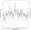 |
Fig. 9 Same as Fig. 8 but for the potassium line (7698.96 Å). |
| In the text | |
 |
Fig. 10 Same as Fig. 8 but for the lithium line (6707.76 Å). |
| In the text | |
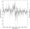 |
Fig. 11 Same as Fig. 8 but for the H-α line (6562.82Å). |
| In the text | |
|
Fig. 12 Detectability map based on a Gaussian fit for a set of binary CCFs with temperature ranging from 100 to 3000 K and including from the 100 to 3000 strongest water lines. |
| In the text | |
|
Fig. 13 Measured CCFs in the planet rest frame with water vapor mask at 1400 K and 1600 lines for both nights (left panel: 2019-02-24 and middle panel: 2019-03-17) and the combination of them (right panel). Right panel: combined CCF with the highest confidence level from the map of temperature vs. number lines (600 K and 1900 lines; Fig. 12) has been added in gray. |
| In the text | |
|
Fig. 14 Low-resolution model described in Sect. 7.1 with different cut in pressure to represent various gray cloud-decks (colored curves). In black, the HST data from Spake et al. (2020). The inset is the same as in Fig. 6 (right panel) where we added the high-resolution model Na doublet lines (green) which are not affected by the cloud-deck pressure. |
| In the text | |
|
Fig. 15 Combining low- and high-resolution datasets. The color-code is the same as in Fig. 14. Left column: ESPRESSO CCFs with injected models retrieved for the equilibrium temperature and 1600 lines. The best Gaussian-fit model shown in black evaluates whether or not the injected model could be retrieved in the ESPRESSOdata. Middle column: high-resolution model that is injected into the ESPRESSO data. Right column: HST data in black are compared to low-resolution models. A minimization algorithm is applied to estimate the
|
| In the text | |
|
Fig. B.1 Cross correlation functions for the ExoMol BT2 (top panel), the ExoMol Pokazatel (middle panel), and the HITEMP2010 (bottom panel) with a water binary mask at 1400 K and 1600 lines. |
| In the text | |
|
Fig. C.1 Map of temperature vs. number of lines representing the Gaussian fit outputs for each CCF set. From top to bottom: detection level, amplitude, FWHM, and centroid position. |
| In the text | |
|
Fig. C.2 Measured CCF with the injected model with the water vapor mask at 1400 K and 1600 lines in blue. The same mask is used to compute the modeled CCF shown in orange. This mask is used as it maximizes the detection level with the temperature fixed to Teq. |
| In the text | |
|
Fig. D.1 Radial velocities of WASP-127b for both transits (respectively blue and orange for the 2019-02-24 and 2019-03-17) phased-folded. The radial velocities have been corrected from the vsyst and the Keplerian model. The vertical dashed line is the mid-transit while the dense vertical dotted lines correspond to t1 and t4 and the vertical dotted lines are t2 and t3. The horizontal dashed line corresponds to null velocity. |
| In the text | |
|
Fig. E.1 Transmission spectrum with (blue) or without (orange) the RASSINE normalization for the 2019-02-24 transit. |
| In the text | |
Current usage metrics show cumulative count of Article Views (full-text article views including HTML views, PDF and ePub downloads, according to the available data) and Abstracts Views on Vision4Press platform.
Data correspond to usage on the plateform after 2015. The current usage metrics is available 48-96 hours after online publication and is updated daily on week days.
Initial download of the metrics may take a while.