| Issue |
A&A
Volume 644, December 2020
|
|
|---|---|---|
| Article Number | A67 | |
| Number of page(s) | 7 | |
| Section | Stellar atmospheres | |
| DOI | https://doi.org/10.1051/0004-6361/202039167 | |
| Published online | 01 December 2020 | |
Ca II H&K stellar activity parameter: a proxy for extreme ultraviolet stellar fluxes★
1
Space Research Institute, Austrian Academy of Sciences,
Schmiedlstrasse 6,
8042
Graz, Austria
e-mail: This email address is being protected from spambots. You need JavaScript enabled to view it.
2
Laboratory for Atmospheric and Space Physics, University of Colorado,
UCB 600,
Boulder,
CO
80309, USA
Received:
12
August
2020
Accepted:
28
October
2020
Abstract
Atmospheric escape is an important factor shaping the exoplanet population and hence drives our understanding of planet formation. Atmospheric escape from giant planets is driven primarily by the stellar X-ray and extreme ultraviolet (EUV) radiation. Furthermore, EUV and longer wavelength UV radiation power disequilibrium chemistry in the middle and upper atmospheres. Our understanding of atmospheric escape and chemistry, therefore, depends on our knowledge of the stellar UV fluxes. While the far-ultraviolet (FUV) fluxes can be observed for some stars, most of the EUV range is unobservable due to the lack of a space telescope with EUV capabilities and, for the more distant stars, due to interstellar medium absorption. Therefore, it becomes essential to have an indirect means for inferring EUV fluxes from features observable at other wavelengths. We present here analytic functions for predicting the EUV emission of F-, G-, K-, and M-type stars from the log R′HK activity parameter that is commonly obtained from ground-based optical observations of the Ca II H&K lines. The scaling relations are based on a collection of about 100 nearby stars with published log R′HK and EUV flux values, the latter of which are either direct measurements or inferences from high-quality FUV spectra. The scaling relations presented here return EUV flux values with an accuracy of about a factor of three, which is slightly lower than that of other similar methods based on FUV or X-ray measurements.
Key words: ultraviolet: stars / stars: chromospheres / planet-star interactions / stars: late-type / stars: activity planets and satellites: atmospheres
Full Table 1 is available at the CDS via anonymous cdsarc.u-strasbg.fr (130.79.128.5) or via http://cdsarc.u-strasbg.fr/viz-bin/cat/J/A+A/644/A67
© ESO 2020
1 Introduction
Planet atmospheric escape is one of the most important processes affecting the evolution of planetary atmospheres (e.g. Lopez & Fortney 2013; Owen & Wu 2013; Jin et al. 2014), and it has played a key role in shaping the atmospheres of the inner Solar System planets (e.g. Lammer et al. 2018, 2020). It is believed that escape also has a profound impact on the observed exoplanet population (e.g. Owen & Wu 2017; Jin & Mordasini 2018). Furthermore, because of the difficulty in directly observing and studying young planets, constraining atmospheric accretion processes requires tracing the evolution, and hence mass loss, of older planets, which can instead be more easily characterised observationally (e.g. Jin et al. 2014; Kubyshkina et al. 2018a, 2019a,b).
The vast majority of the known exoplanets orbit close to their host stars and are therefore strongly irradiated. Except in specific cases (e.g. very young or atmosphereless planets; Owen & Wu 2016; Fossati et al. 2017a; Vidotto et al. 2018), escape is mainly driven by heating due to absorption of the stellar high-energy radiation, in particular extreme ultraviolet (EUV) and X-ray photons, together called XUV (e.g. Watson et al. 1981; Lammer et al. 2003; Yelle 2004; Murray-Clay et al. 2009; Koskinen et al. 2013a,b). The XUV photons can heat the thermosphere to temperatures of the order of 104 K, which causes the atmosphere to expand, possibly hydrodynamically, leading to mass loss. For classical hot Jupiters (e.g. HD 209458b), mass-loss rates are of the order of 109−10 g s−1, but they can become significantly larger for planets orbiting hot stars (e.g. Fossati et al. 2018b; García Muñoz & Schneider 2019; Mitani et al. 2020), for planets orbiting young, active stars (e.g. Penz et al. 2008; Kubyshkina et al. 2018b), and for low-gravity planets (e.g. Lammer et al. 2016; Cubillos et al. 2017).
Atmospheric escape has been directly observed for a few close-in exoplanets (e.g. Vidal-Madjar et al. 2003; Fossati et al. 2010; Linsky et al. 2010; Lecavelier des Etangs et al. 2012; Haswell et al. 2012; Ehrenreich et al. 2015; Bourrier et al. 2018; Mansfield et al. 2018; Sing et al. 2019; Cubillos et al. 2020) and predicted for many others (e.g. Ehrenreich & Désert 2011; Salz et al. 2016); however, to extract the relevant information from the observations and/or to theoretically estimate the physical conditions of planetary upper atmospheres and infer mass-loss rates, it is necessary to quantify the amount of XUV flux irradiating the planet. Because of the lack of an observational facility with adequate capabilities (France et al. 2019) and due to interstellar medium absorption for more distant stars, it is not possible to directly observe the EUV stellar emission for stars other than the Sun. Although there are a few space telescopes with X-ray capabilities, the X-ray stellar emission is typically an order of magnitude less intense than the EUV emission and has a smaller absorption cross-section in a hydrogen-dominated atmosphere (e.g. Cecchi-Pestellini et al. 2009; Sanz-Forcada et al. 2011; Tu et al. 2015), making the X-ray fluxes alone inadequate for constraining upper atmospheres and escape.
Several methods and scaling relations have been devised to estimate stellar XUV fluxes from proxies observable at longer or shorter wavelengths, such as X-ray and ultraviolet (UV) fluxes (e.g. Sanz-Forcada et al. 2011; Linsky et al. 2014; Chadney et al. 2015; Louden et al. 2017; France et al. 2018). For example, Linsky et al. (2014) derived a correlation between EUV and Lyα emission fluxes to use observations of the Lyα line to infer stellar XUV fluxes in different bands. In their work, Linsky et al. (2014) employed a mixture of EUV spectra that had previously been measured by the Extreme Ultraviolet Explorer (EUVE) for a few nearby stars and solar spectral synthesis computations. Linsky et al. (2013) further derived similar correlations between the fluxes of the Lyα line and several emission features in the UV (CII, CIV, OI, MgII h&k lines) and optical (Ca II H&K lines) bands. However, these scaling relations require either reconstructing the Lyα line, whose core is typically heavily absorbed by the interstellar medium, or employing two scaling relations to derive the stellar XUV fluxes from emission lines other than Lyα. More recently, France et al. (2018) followed the same strategy from Linsky et al. (2014), deriving a correlation between EUV emission fluxes in two bands (i.e. 90–360 and 90–911 Å) and lines in the far-ultraviolet (NV and SiIV), for which high-quality spectra had been collected with the Hubble Space Telescope. The advantage of the France et al. (2018) relation over that of Linsky et al. (2013, 2014) is the larger sample and the use of lines forming at temperatures closer to that of the EUV formation temperature range. Other works have reconstructed stellar EUV spectra by scaling the solar UV spectrum to match measurements of high-energy far-ultraviolet (FUV) emission lines (e.g. Fossati et al. 2015, 2018a). X-ray and FUV measurements have also been combined via the differential emission measure (e.g. Louden et al. 2017) or by scaling the observed XUV fluxes of nearby stars (e.g. Chadney et al. 2015).
All of these EUV estimation methods require space-based observations at FUV and/or X-ray wavelengths, which are not easy to obtain, particularly for large samples of stars. One way around this problem is to employ the stellar rotation rate as a proxy for activity, hence XUV emission, of late-type stars (e.g. Johnstone et al. 2015; Tu et al. 2015); however, this method is less accurate than those based on the direct measurement of chromospheric and/or coronal emission, and it has never been empirically verified, except for Sun-like stars (e.g. Ribas et al. 2005). Furthermore, this method may in some cases lead to incorrect conclusions, such as for the planet-hosting star WASP-18, which is a fast rotator but has an extremely low activity level that is believed to be dampened by tidal interactions with the massive close-in planet (Fossati et al. 2018a).
We employ here the stellar sample from France et al. (2018) to derive the correlation between the  stellar activity index and EUV fluxes in the 90–911 Å wavelength range. The
  index is a measure of the stellar chromospheric emission flux at the core of the deep Ca II H&K absorption lines (~3933 and ~3968 Å), which has the advantage of lying in the optical band and therefore of being easily observable from the ground. However,
  has the disadvantage of forming mostly in the chromosphere, hence at lower temperatures compared to the typical formation temperature of the EUV stellar emission. A large number of studies have made and continue to make use of the
  index, which has its roots in the Mount Wilson S-index (SMW), to study stellar activity (e.g. Wilson 1978; Noyes et al. 1984; Duncan et al. 1991; Baliunas et al. 1995). In this work, we obtain scaling relations that allow for the inference of EUV fluxes for M-, K-, G-, and F-type stars directly from the
  index. This in turn allows for the inference – in a simple, direct way – of the EUV emission of a large number of late-type stars without the need for high-quality space-based observations.
This paper is organised as follows. Section 2 presents the considered sample of stars employed to derive the  EUV correlation. Section 3 presents the
  EUV correlation, and we discuss the results and conclusions of this work in Sect. 4.
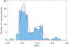 |
Fig. 1 Distribution of the median |


2 Stellar sample and stellar parameters
We started by considering the stars comprising the sample of France et al. (2018): 104 F-, G-, K-, and M-type stars lying within about 50 pc.For each star, France et al. (2018) estimated the EUV emission flux in the 90–360 Å wavelength range on the basis of FUV observations, in particular the NV and SiIV lines as well as the stellar bolometric flux at Earth (Fbol). These EUV estimates have an accuracy of about a factor of two and are based on relationships between the fractional FUV emission line luminosity and the fractional EUV luminosity they obtained from moderate-to-high quality EUV spectra in the 90–360 Å wavelength range collected by the EUVE satellite.
For each star in the France et al. (2018) sample, we collected measurements of the  activity parameter from the literature and retained only the stars for which we found at least one measurement (Isaacson & Fischer 2010; Boro Saikia et al. 2018; Jenkins et al. 2011, 2006; Caillault et al. 1991; Mamajek & Hillenbrand 2008; Gray et al. 2006, 2003; Moutou et al. 2014; Arriagada 2011; Robertson et al. 2012; Anderson et al. 2014; Wittenmyer et al. 2009; Laws et al. 2003; Henry et al. 1996; Canto Martins et al. 2011; Pace 2013; Astudillo-Defru et al. 2017; Hinkel et al. 2017; Ment et al. 2018; Wright et al. 2004; Hall et al. 2009; Morris et al. 2017). The total number of collected
  measurements is 498. The distribution of the median
  values used in this work is shown in Fig. 1. The distribution appears to be bimodal, with peaks at
  values of about −5.0 and −4.5, and hence it is similar to the overall distribution of
  values of stars in the solar neighbourhood (e.g. Vaughan & Preston 1980; Gray et al. 2003).
For each star, we identified and removed outlier  values by employing a two-step approach. First, we removed all
  values lower than − 5.1 (a total of 28 removed measurements for 17 different stars of spectral types G, K, and M), which is the minimum
  value (i.e. usually called “basal level”) possible for main sequence late-type stars (Wright et al. 2004). However, we remark that the sample from Wright et al. (2004) was mostly composed of F-, G-, and K-type stars and that several M dwarfs present
  values below the basal level of −5.1 (e.g. Astudillo-Defru et al. 2017); this may be due to the fact that Astudillo-Defru et al. (2017) focused on planet-hosting stars that are typically inactive because of selection biases and/or the fact that M-type stars may have a basal level different from that of hotter solar-like stars. Second, we excluded further outliers by identifying the
  values that deviate by more than three times the median absolute deviation (MAD) from the median value. We then calculated the average and median from the remaining
  measurements (Table 1). Figure 1 presents the distribution of median
  values obtained for each star following the removal of the outliers and compares it with the original distribution. It shows that the removal of the outliers has not significantly modified the underlying distribution, which remains bimodal. We confirmed the bimodality of the distribution by fitting it employing a double-peaked Gaussian (shown in Fig. 1) and by running a Kolmogorov-Smirnov test on the two resultant Gaussian distributions; we found that, at high significance, they are indeed drawn from distinct samples. Furthermore, because of the close distance of the stars in our sample, the
  values are not systematically depressed by interstellar medium absorption (Fossati et al. 2017b). This process led to a sample comprising 96 stars.
Figure 2 presents the standard deviation of the  values for each star, following the removal of the outliers, as a function of the median
  value. Except for one star, HD 106516, the standard deviation is smaller than 0.1 and the median value of the standard deviation is about 0.04. Since the scatter on the standard deviation does not increase with increasing
  values, the scatter is most likely driven by measurement uncertainties rather than by stellar variability. Therefore, for each star, we took the standard deviation as the uncertainty on the median
  value, and, for the stars with only one measured
  value, we considered the median value of the standard deviation (i.e. ~0.04) as the uncertainty on the measured
  value. By taking the median
  value, we mitigate the effects on the results of the intrinsic stellar variability and non-simultaneity of the
  and EUV measurements.
Figure 3 presents the distribution of the median  values as a function of the stellar effective temperature (Teff) obtained from the Gaia DR2 catalogue (Gaia Collaboration 2018). Stellar temperature values from France et al. (2018) were retained for stars where temperature information was absent in the Gaia DR2 catalogue. This plot further shows the uncertainty as well as the minimum and maximum values associated with each point. Following the outlier removal based on the MAD, the median
  value for most stars lies roughly in the middle between the minimum and maximum values, as expected. The majority of the stars are G-type, but M-types and late F-types are also well represented; there are relatively few early or mid K-type stars.
For each considered star, we updated Teff, the stellar distance (d), and the stellar radius, hence the bolometric flux at Earth, using the values given in the Gaia DR2 catalogue (Gaia Collaboration 2018). The stellar radii were updated using the Gaia stellar magnitudes, effective temperatures, and distances as follows:
 (1)
(1)
where Rstar is the stellar radius, Rsun is the solar radius, Teff,sun is the solar effective temperature(5777 K), Teff,star is the stellar effective temperature, dstar is the distance to the star, dsun is the distance to the Sun, msun is the solar apparent V -band magnitude (−26.73), and mstar is the apparent stellar V -band magnitude. This equation assumes that the stellar apparent magnitude is not affected by interstellar extinction, which we assume to be the case given the close distance to the stars in our sample.
Our reference sample of stars is that of France et al. (2018), which is also our source for the stellar EUV fluxes at Earth. However, for most stars, we updated both the Teff and radius, hence the bolometric fluxes at Earth. For this reason, except for the stars for which the EUV flux originates from EUVE observations, we employed the scaling relations from France et al. (2018, their Eqs. (4)–(6)) as well as their NV flux measurements to update the stellar EUV fluxes that are listed in Table 1. For the stars without an NV flux measurement, we employed the SiIV flux measurement. Figure 4 shows the difference between the EUV fluxes given by France et al. (2018) and those we obtained following the update of the bolometric fluxes at Earth. The median difference is about 2%, and, for most stars, the difference lies within 10%.
List of selected targets in order of spectral type from F- to M-type, as well as their basic parameters,  values, and EUV fluxes.
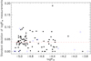 |
Fig. 2 Standard deviation obtained from the |


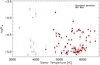 |
Fig. 3 Median |


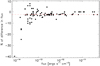 |
Fig. 4 Difference in EUV flux at Earth values in the 90–360 Å wavelength range between those given by France et al. (2018) and those obtained by employing the scaling relation in France et al. (2018, Eqs. (4)–(6)) as well as the stellar parameters derived from the Gaia DR2 catalogue. The median difference is about 2% (red dashed line). Except for stars with low EUV fluxes (below 2 × 10⁻¹⁴ erg cm−2 s−1) the difference is within 10%. |
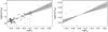 |
Fig. 5 Correlation between the stellar activity index ( |

3 Results
Figure 5 shows the stellar EUV flux as a function of the median  value for the stars in our sample and the best linear fit through these points. The linear fit was achieved with a minimised chi-square approach that accounts for the uncertainties on both EUV fluxes and
  values. To improve the robustness of the fits, we employed an iterative sigma clipping algorithm to remove stars that deviated by more than 1.5 times the root mean square (RMS) value from the fit. We ran separate fits for stars belonging to different spectral types. We found that the EUV flux versus
  value correlation is comparable for F-, G-, and K-type stars and therefore considered all three for the joint fit; however, the M-type stars appearto follow a different scaling relation. We remark, though, that M dwarfs later than M3.5 are fully convective and may not behave like the earlier M dwarfs in terms of chromospheric and coronal emission, but the excessively small sample does not allow us to identify statistically significant differences when performing separate fits.
We find that the correlation between the stellar activity index ( ) and the EUV flux in the 90−911 Å wavelength range can be described by a linear fit of the form
 (2)
(2)
where the c1 and c2 coefficients are listed in Table 2. We further compute the Pearson correlation coefficients (PCCs) for  versus log (EUV∕Fbol), finding that the linear correlations are indeed significant (see values in Table 2). The results indicate that the correlation for F-, G-, and K-type stars is significantly steeper than that for M-type stars, which is in agreement with what has previously been found (see e.g. Linsky et al. 2013, 2014; France et al. 2018). These results also indicate that our scaling relations provide EUV fluxes with an accuracy of about a factor of three, which is slightly higher than that of other similar methodsbased on FUV or X-ray measurements. The scatter present in the line fits has the largest contribution to the uncertainties in the EUV flux estimates.
4 Discussion and conclusion
We presented here a linear correlation between the  stellar activity index and the EUV flux emitted by late-type stars in the 90−911 Å wavelength range, which is responsible for most of the heating in upper planetary atmospheres. This correlation enables one to convert the chromospheric emission at the core of the Ca II H&K lines, parameterised by the
  value and measurable from the ground, into stellar high-energy emission that can then be used to estimate, for example, exoplanetary atmosphericmass-loss rates.
Before this work, one could have also combined the scaling relations published by Linsky et al. (2013, 2014) to convert the chromospheric emission at the line core into EUV fluxes, though this would have implied first converting the  value into Ca II H&K chromospheric emission and then passing it through the estimation of the Lyα fluxes. Therefore, we compared the
  versus EUV fluxes obtained following that approach as well as this work’s method (presented in Sect. 3). To this end, we first converted the
  values into disk-integrated chromospheric emission flux in erg cm−2 s−1 following Fossati et al. (2017b) and Sreejith et al. (2019). In short, the disk-integrated Ca II H&K chromospheric line emission at a distance of 1 AU (FHK(1 AU)) is (see Sect. 2 of Fossati et al. 2017b):
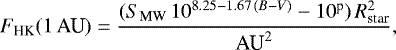 (3)
(3)
where SMW is the S-index activity indicator in the Mount-Wilson system (Noyes et al. 1984; Mittag et al. 2013), Rstar is the stellar radius in cm, and AU is one astronomical unit in cm. The exponent p in Eq. (3) is equal to 7.49 − 2.06 (B − V) for main sequence stars with 0.44 ≤ B − V < 1.28 and is equal to 6.19 − 1.04 (B − V) for main sequence stars with 1.28 ≤ B − V < 1.60 (Mittag et al. 2013), while the SMW index is defined as:
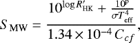 (4)
(4)
where Ccf is (Rutten 1984)
 (5)
(5)
The parameters employed to derive FHK(1 AU) are listed in Table 1, and the B − V values were obtained from the stellar effective temperature by interpolating Table 51 from Pecaut & Mamajek (2013).
We then set an array of  values, converted them to FHK(1 AU) as described above, and used the scaling relations from Linsky et al. (2013) to obtain the Lyα fluxes, which we then converted into EUV fluxes in the 100 to 912 Å range by employing the scaling relations from Linsky et al. (2014). We followed this procedure separately for F5, G5, K5, and M0 stars. Figure 6 shows a comparison between the EUV
 correlations obtained by combining the scaling relations from Linsky et al. (2013, 2014) and the two linear fits derived in this work, including the uncertainties on the fits.
We find that our fit for F-, G-, K-, M-type stars is significantly steeper than that obtained by combining the scaling relations from Linsky et al. (2013, 2014). For active stars, the two correlations lead to comparable results, while, as a consequence of the different slopes, a difference of up to about 1.5 orders of magnitude can be observed for inactive F-, G-, K-type stars, and a difference of the order of less than one magnitude can be observed in the case of inactive M-type stars. We also followed the original formalism described by Noyes et al. (1984) to compute FHK(1 AU) from the  values and found no significant differences from the results described above.
In an attempt to understand the origin of these differences, we took from Linsky et al. (2014) the EUV fluxes of the stars that are also part of our sample and plot their position in Fig. 6, finding that they follow our EUV versus  fits. To further trace the origin of this difference, we compared the Ca II H&K chromospheric emission flux at 1 AU, which was calculated from
  using the method described above and the values given by Linsky et al. (2013, their Table 4). The comparison is shown in Fig. 7. Indeed, Eq. (3) appears to overestimate the Ca II H&K chromospheric emission flux at 1 AU, particularly for the less active stars. This further comparison suggests that the difference may be due to the fact that Eq. (3) does not account for the extra chromospheric emission flux that falls outside the band employed to measure SMW values, and hence the
  values (Hartmann et al. 1984). In other words, the wavelength bands used to estimate the
  values differ from the FHK(1 AU) values employed by Linsky et al. (2013). Therefore, deriving FHK(1 AU) from the
  value and then employing the Linsky et al. (2013, 2014) scaling relations may significantly overestimate the EUV fluxes, and hence our Eq. (2) should be used instead. Our results can therefore be used to estimate wavelength-integrated stellar EUV fluxes for stars for which X-ray or FUV observations are either not available or not possible, hence enabling one to more accurately study, for example, the upper atmospheres of planets orbiting late-type stars and their interaction with their host stars.

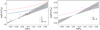 |
Fig. 6 Correlation between EUV and |


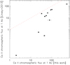 |
Fig. 7 Comparison between Ca II H&K chromospheric emission flux at 1 AU calculated from
|

Acknowledgements
A.G.S. and L.F. acknowledge financial support from the Austrian Forschungsförderungsgesellschaft FFG project CONTROL P865968. We thank the anonymous referee for the comments that led to improving the manuscript. This research has made use of the VizieR catalogue access tool, CDS, Strasbourg, France (DOI: 10.26093/cds/vizier). The original description of the VizieR service was published in Ochsenbein et al. (2000).
References
- Anderson, D. R., Collier Cameron, A., Delrez, L., et al. 2014, MNRAS, 445, 1114 [NASA ADS] [CrossRef] [Google Scholar]
- Arriagada, P. 2011, ApJ, 734, 70 [NASA ADS] [CrossRef] [Google Scholar]
- Astudillo-Defru, N., Delfosse, X., Bonfils, X., et al. 2017, A&A, 600, A13 [NASA ADS] [CrossRef] [EDP Sciences] [Google Scholar]
- Baliunas, S. L., Donahue, R. A., Soon, W. H., et al. 1995, ApJ, 438, 269 [NASA ADS] [CrossRef] [Google Scholar]
- Boro Saikia, S., Marvin, C. J., Jeffers, S. V., et al. 2018, A&A, 616, A108 [NASA ADS] [CrossRef] [EDP Sciences] [Google Scholar]
- Bourrier, V., Lecavelier des Etangs, A., Ehrenreich, D., et al. 2018, A&A, 620, A147 [NASA ADS] [CrossRef] [EDP Sciences] [Google Scholar]
- Caillault, J.-P., Vilhu, O., & Linsky, J. L. 1991, ApJ, 383, 594 [CrossRef] [Google Scholar]
- Canto Martins, B. L., Das Chagas, M. L., Alves, S., et al. 2011, A&A, 530, A73 [NASA ADS] [CrossRef] [EDP Sciences] [Google Scholar]
- Cecchi-Pestellini, C., Ciaravella, A., Micela, G., & Penz, T. 2009, A&A, 496, 863 [NASA ADS] [CrossRef] [EDP Sciences] [Google Scholar]
- Chadney, J. M., Galand, M., Unruh, Y. C., Koskinen, T. T., & Sanz-Forcada, J. 2015, Icarus, 250, 357 [NASA ADS] [CrossRef] [Google Scholar]
- Cubillos, P., Erkaev, N. V., Juvan, I., et al. 2017, MNRAS, 466, 1868 [NASA ADS] [CrossRef] [Google Scholar]
- Cubillos, P. E., Fossati, L., Koskinen, T., et al. 2020, AJ, 159, 111 [Google Scholar]
- Duncan, D. K., Vaughan, A. H., Wilson, O. C., et al. 1991, ApJS, 76, 383 [NASA ADS] [CrossRef] [Google Scholar]
- Ehrenreich, D., & Désert, J. M. 2011, A&A, 529, A136 [NASA ADS] [CrossRef] [EDP Sciences] [Google Scholar]
- Ehrenreich, D., Bourrier, V., Wheatley, P. J., et al. 2015, Nature, 522, 459 [Google Scholar]
- Fossati, L., Haswell, C. A., Froning, C. S., et al. 2010, ApJ, 714, L222 [Google Scholar]
- Fossati, L., France, K., Koskinen, T., et al. 2015, ApJ, 815, 118 [NASA ADS] [CrossRef] [Google Scholar]
- Fossati, L., Erkaev, N. V., Lammer, H., et al. 2017a, A&A, 598, A90 [NASA ADS] [CrossRef] [EDP Sciences] [Google Scholar]
- Fossati, L., Marcelja, S. E., Staab, D., et al. 2017b, A&A, 601, A104 [NASA ADS] [CrossRef] [EDP Sciences] [Google Scholar]
- Fossati, L., Koskinen, T., France, K., et al. 2018a, AJ, 155, 113 [NASA ADS] [CrossRef] [Google Scholar]
- Fossati, L., Koskinen, T., Lothringer, J. D., et al. 2018b, ApJ, 868, L30 [NASA ADS] [CrossRef] [Google Scholar]
- France, K., Arulanantham, N., Fossati, L., et al. 2018, ApJS, 239, 16 [CrossRef] [Google Scholar]
- France, K., Fleming, B. T., Drake, J. J., et al. 2019, SPIE Conf. Ser., 11118, 1111808 [Google Scholar]
- Gaia Collaboration (Brown, A. G. A., et al.) 2018, A&A, 616, A1 [NASA ADS] [CrossRef] [EDP Sciences] [Google Scholar]
- García Muñoz, A., & Schneider, P. C. 2019, ApJ, 884, L43 [CrossRef] [Google Scholar]
- Gray, R. O., Corbally, C. J., Garrison, R. F., McFadden, M. T., & Robinson, P. E. 2003, AJ, 126, 2048 [NASA ADS] [CrossRef] [Google Scholar]
- Gray, R. O., Corbally, C. J., Garrison, R. F., et al. 2006, AJ, 132, 161 [NASA ADS] [CrossRef] [Google Scholar]
- Hall, J. C., Henry, G. W., Lockwood, G. W., Skiff, B. A., & Saar, S. H. 2009, AJ, 138, 312 [NASA ADS] [CrossRef] [Google Scholar]
- Hartmann, L., Soderblom, D. R., Noyes, R. W., Burnham, N., & Vaughan, A. H. 1984, ApJ, 276, 254 [NASA ADS] [CrossRef] [Google Scholar]
- Haswell, C. A., Fossati, L., Ayres, T., et al. 2012, ApJ, 760, 79 [Google Scholar]
- Henry, T. J., Soderblom, D. R., Donahue, R. A., & Baliunas, S. L. 1996, AJ, 111, 439 [NASA ADS] [CrossRef] [Google Scholar]
- Hinkel, N. R., Mamajek, E. E., Turnbull, M. C., et al. 2017, ApJ, 848, 34 [NASA ADS] [CrossRef] [Google Scholar]
- Isaacson, H., & Fischer, D. 2010, ApJ, 725, 875 [NASA ADS] [CrossRef] [Google Scholar]
- Jenkins, J. S., Jones, H. R. A., Tinney, C. G., et al. 2006, MNRAS, 372, 163 [NASA ADS] [CrossRef] [Google Scholar]
- Jenkins, J. S., Murgas, F., Rojo, P., et al. 2011, A&A, 531, A8 [NASA ADS] [CrossRef] [EDP Sciences] [Google Scholar]
- Jin, S., & Mordasini, C. 2018, ApJ, 853, 163 [NASA ADS] [CrossRef] [Google Scholar]
- Jin, S., Mordasini, C., Parmentier, V., et al. 2014, ApJ, 795, 65 [Google Scholar]
- Johnstone, C. P., Güdel, M., Brott, I., & Lüftinger, T. 2015, A&A, 577, A28 [NASA ADS] [CrossRef] [EDP Sciences] [Google Scholar]
- Koskinen, T. T., Harris, M. J., Yelle, R. V., & Lavvas, P. 2013a, Icarus, 226, 1678 [Google Scholar]
- Koskinen, T. T., Yelle, R. V., Harris, M. J., & Lavvas, P. 2013b, Icarus, 226, 1695 [NASA ADS] [CrossRef] [Google Scholar]
- Kubyshkina, D., Fossati, L., Erkaev, N. V., et al. 2018a, A&A, 619, A151 [NASA ADS] [CrossRef] [EDP Sciences] [Google Scholar]
- Kubyshkina, D., Lendl, M., Fossati, L., et al. 2018b, A&A, 612, A25 [NASA ADS] [CrossRef] [EDP Sciences] [Google Scholar]
- Kubyshkina, D., Cubillos, P. E., Fossati, L., et al. 2019a, ApJ, 879, 26 [NASA ADS] [CrossRef] [Google Scholar]
- Kubyshkina, D., Fossati, L., Mustill, A. J., et al. 2019b, A&A, 632, A65 [CrossRef] [EDP Sciences] [Google Scholar]
- Lammer, H., Selsis, F., Ribas, I., et al. 2003, ApJ, 598, L121 [Google Scholar]
- Lammer, H., Erkaev, N. V., Fossati, L., et al. 2016, MNRAS, 461, L62 [NASA ADS] [CrossRef] [Google Scholar]
- Lammer, H., Zerkle, A. L., Gebauer, S., et al. 2018, A&ARv, 26, 2 [NASA ADS] [CrossRef] [Google Scholar]
- Lammer, H., Leitzinger, M., Scherf, M., et al. 2020, Icarus, 339, 113551 [CrossRef] [Google Scholar]
- Laws, C., Gonzalez, G., Walker, K. M., et al. 2003, AJ, 125, 2664 [NASA ADS] [CrossRef] [Google Scholar]
- Lecavelier des Etangs, A., Bourrier, V., Wheatley, P. J., et al. 2012, A&A, 543, L4 [NASA ADS] [CrossRef] [EDP Sciences] [Google Scholar]
- Linsky, J. L., Yang, H., France, K., et al. 2010, ApJ, 717, 1291 [Google Scholar]
- Linsky, J. L., France, K., & Ayres, T. 2013, ApJ, 766, 69 [NASA ADS] [CrossRef] [Google Scholar]
- Linsky, J. L., Fontenla, J., & France, K. 2014, ApJ, 780, 61 [NASA ADS] [CrossRef] [Google Scholar]
- Lopez, E. D., & Fortney, J. J. 2013, ApJ, 776, 2 [Google Scholar]
- Louden, T., Wheatley, P. J., & Briggs, K. 2017, MNRAS, 464, 2396 [NASA ADS] [CrossRef] [Google Scholar]
- Mamajek, E. E., & Hillenbrand, L. A. 2008, ApJ, 687, 1264 [NASA ADS] [CrossRef] [Google Scholar]
- Mansfield, M., Bean, J. L., Oklopčić, A., et al. 2018, ApJ, 868, L34 [Google Scholar]
- Ment, K., Fischer, D. A., Bakos, G., Howard, A. W., & Isaacson, H. 2018, AJ, 156, 213 [NASA ADS] [CrossRef] [Google Scholar]
- Mitani, H., Nakatani, R., & Yoshida, N. 2020, ApJ, submitted [arXiv:2005.08676] [Google Scholar]
- Mittag, M., Schmitt, J. H. M. M., & Schröder, K. P. 2013, A&A, 549, A117 [NASA ADS] [CrossRef] [EDP Sciences] [Google Scholar]
- Morris, B. M., Hawley, S. L., Hebb, L., et al. 2017, ApJ, 848, 58 [NASA ADS] [CrossRef] [Google Scholar]
- Moutou, C., Hébrard, G., Bouchy, F., et al. 2014, A&A, 563, A22 [NASA ADS] [CrossRef] [EDP Sciences] [Google Scholar]
- Murray-Clay, R. A., Chiang, E. I., & Murray, N. 2009, ApJ, 693, 23 [Google Scholar]
- Noyes, R. W., Hartmann, L. W., Baliunas, S. L., Duncan, D. K., & Vaughan, A. H. 1984, ApJ, 279, 763 [NASA ADS] [CrossRef] [Google Scholar]
- Ochsenbein, F., Bauer, P., & Marcout, J. 2000, A&AS, 143, 23 [NASA ADS] [CrossRef] [EDP Sciences] [Google Scholar]
- Owen, J. E., & Wu, Y. 2013, ApJ, 775, 105 [Google Scholar]
- Owen, J. E., & Wu, Y. 2016, ApJ, 817, 107 [NASA ADS] [CrossRef] [Google Scholar]
- Owen, J. E., & Wu, Y. 2017, ApJ, 847, 29 [Google Scholar]
- Pace, G. 2013, A&A, 551, L8 [NASA ADS] [CrossRef] [EDP Sciences] [Google Scholar]
- Pecaut, M. J., & Mamajek, E. E. 2013, ApJS, 208, 9 [Google Scholar]
- Penz, T., Micela, G., & Lammer, H. 2008, A&A, 477, 309 [NASA ADS] [CrossRef] [EDP Sciences] [Google Scholar]
- Ribas, I., Guinan, E. F., Güdel, M., & Audard, M. 2005, ApJ, 622, 680 [NASA ADS] [CrossRef] [Google Scholar]
- Robertson, P., Endl, M., Cochran, W. D., et al. 2012, ApJ, 749, 39 [NASA ADS] [CrossRef] [Google Scholar]
- Rutten, R. G. M. 1984, A&A, 130, 353 [NASA ADS] [Google Scholar]
- Salz, M., Czesla, S., Schneider, P. C., & Schmitt, J. H. M. M. 2016, A&A, 586, A75 [NASA ADS] [CrossRef] [EDP Sciences] [Google Scholar]
- Sanz-Forcada, J., Micela, G., Ribas, I., et al. 2011, A&A, 532, A6 [NASA ADS] [CrossRef] [EDP Sciences] [Google Scholar]
- Sing, D. K., Lavvas, P., Ballester, G. E., et al. 2019, AJ, 158, 91 [Google Scholar]
- Sreejith, A. G., Fossati, L., Fleming, B. T., et al. 2019, J. Astron. Telesc. Instrum. Syst., 5, 018004 [CrossRef] [Google Scholar]
- Tu, L., Johnstone, C. P., Güdel, M., & Lammer, H. 2015, A&A, 577, L3 [NASA ADS] [CrossRef] [EDP Sciences] [Google Scholar]
- Vaughan, A. H., & Preston, G. W. 1980, PASP, 92, 385 [NASA ADS] [CrossRef] [Google Scholar]
- Vidal-Madjar, A., Lecavelier des Etangs, A., Désert, J. M., et al. 2003, Nature, 422, 143 [Google Scholar]
- Vidotto, A. A., Lichtenegger, H., Fossati, L., et al. 2018, MNRAS, 481, 5296 [NASA ADS] [CrossRef] [Google Scholar]
- Watson, A. J., Donahue, T. M., & Walker, J. C. G. 1981, Icarus, 48, 150 [NASA ADS] [CrossRef] [Google Scholar]
- Wilson, O. C. 1978, ApJ, 226, 379 [NASA ADS] [CrossRef] [Google Scholar]
- Wittenmyer, R. A., Endl, M., Cochran, W. D., Levison, H. F., & Henry, G. W. 2009, ApJS, 182, 97 [NASA ADS] [CrossRef] [Google Scholar]
- Wright, J. T., Marcy, G. W., Butler, R. P., & Vogt, S. S. 2004, ApJS, 152, 261 [NASA ADS] [CrossRef] [Google Scholar]
- Yelle, R. V. 2004, Icarus, 170, 167 [NASA ADS] [CrossRef] [Google Scholar]
All Tables
List of selected targets in order of spectral type from F- to M-type, as well as their basic parameters, values, and EUV fluxes.
All Figures
|
Fig. 1 Distribution of the median |
| In the text | |
|
Fig. 2 Standard deviation obtained from the |
| In the text | |
|
Fig. 3 Median |
| In the text | |
|
Fig. 4 Difference in EUV flux at Earth values in the 90–360 Å wavelength range between those given by France et al. (2018) and those obtained by employing the scaling relation in France et al. (2018, Eqs. (4)–(6)) as well as the stellar parameters derived from the Gaia DR2 catalogue. The median difference is about 2% (red dashed line). Except for stars with low EUV fluxes (below 2 × 10⁻¹⁴ erg cm−2 s−1) the difference is within 10%. |
| In the text | |
|
Fig. 5 Correlation between the stellar activity index ( |
| In the text | |
|
Fig. 6 Correlation between EUV and |
| In the text | |
|
Fig. 7 Comparison between Ca II H&K chromospheric emission flux at 1 AU calculated from
|
| In the text | |
Current usage metrics show cumulative count of Article Views (full-text article views including HTML views, PDF and ePub downloads, according to the available data) and Abstracts Views on Vision4Press platform.
Data correspond to usage on the plateform after 2015. The current usage metrics is available 48-96 hours after online publication and is updated daily on week days.
Initial download of the metrics may take a while.