| Issue |
A&A
Volume 644, December 2020
|
|
|---|---|---|
| Article Number | A60 | |
| Number of page(s) | 12 | |
| Section | Stellar structure and evolution | |
| DOI | https://doi.org/10.1051/0004-6361/202038992 | |
| Published online | 01 December 2020 | |
Common-envelope evolution with an asymptotic giant branch star
1
Heidelberger Institut für Theoretische Studien, Schloss-Wolfsbrunnenweg 35, 69118 Heidelberg, Germany
e-mail: This email address is being protected from spambots. You need JavaScript enabled to view it.
2
Max Planck Computing and Data Facility, Gießenbachstr. 2, 85748 Garching, Germany
3
Zentrum für Astronomie der Universität Heidelberg, Astronomisches Rechen-Institut, Mönchhofstr. 12-14, 69120 Heidelberg, Germany
4
Max-Planck-Institut für Astrophysik, Karl-Schwarzschild-Str. 1, 85748 Garching, Germany
5
Zentrum für Astronomie der Universität Heidelberg, Institut für Theoretische Astrophysik, Philosophenweg 12, 69120 Heidelberg, Germany
Received:
21
July
2020
Accepted:
9
October
2020
Abstract
Common-envelope phases are decisive for the evolution of many binary systems. Cases with asymptotic giant branch (AGB) primary stars are of particular interest because they are thought to be progenitors of various astrophysical transients. In three-dimensional hydrodynamic simulations with the moving-mesh code AREPO, we study the common-envelope evolution of a 1.0 M⊙ early-AGB star with companions of different masses. Although the stellar envelope of an AGB star is less tightly bound than that of a red giant, we find that the release of orbital energy of the core binary is insufficient to eject more than about twenty percent of the envelope mass. Ionization energy that is released in the expanding envelope, however, can lead to complete envelope ejection. Because recombination proceeds largely at high optical depths in our simulations, it is likely that this effect indeed plays a significant role in the considered systems. The efficiency of mass loss and the final orbital separation of the core binary system depend on the mass ratio between the companion and the primary star. Our results suggest a linear relation between the ratio of final to initial orbital separation and this parameter.
Key words: hydrodynamics / methods: numerical / stars: AGB and post-AGB / binaries: close
© ESO 2020
1. Introduction
Common envelope (CE) phases, which were first proposed by Paczyński (1976), pose great challenges to binary stellar evolution models. The physical mechanism of these short episodes, where two stellar cores orbit each other inside a giant star’s envelope, is still not well understood. Due to tidal drag, the core binary system transfers orbital energy to the envelope material. This may lead to envelope ejection leaving behind cataclysmic variables, close white-dwarf main-sequence binaries, double white-dwarfs, or other close binary systems of compact stellar cores. Phenomena arising from post-CE binaries include Type Ia supernovae (Iben & Tutukov 1984; Ruiter et al. 2009; Toonen et al. 2012), and also classical novae (Livio et al. 1990), X-ray binaries (Kalogera & Webbink 1998; Taam & Sandquist 2000; Taam & Ricker 2010), white-dwarf mergers (Pakmor et al. 2010; Ruiter et al. 2013), and gravitational wave sources (Belczynski et al. 2002). Moreover, the CE phase is thought to be responsible for the shapes of some planetary nebulae (de Kool 1990; Nordhaus et al. 2007; Hillwig et al. 2016; Bermúdez-Bustamante et al. 2020).
Parameterized descriptions that are typically employed in classical stellar-evolution theory and population-synthesis calculations introduce large uncertainties in the predicted rates of these fundamentally important events. This situation calls for an improved modeling of common-envelope evolution (CEE), which requires a better understanding of the underlying physics and, in particular, the mechanism of envelope ejection that eludes one-dimensional modeling.
We note that CEE (for a review, see Ivanova et al. 2013) starts out with unstable mass transfer and the loss of co-rotation in the progenitor binary system, followed by a rapid inspiral of the secondary star toward the core of the primary star. In this phase, which is sometimes referred to as “plunge-in”, large parts of the orbital energy are thought to be transferred to the envelope. Numerical simulations, however, fail to achieve envelope ejection during the plunge-in when only orbital energy release is considered (e.g., Livio & Soker 1988; Terman et al. 1994; Rasio & Livio 1996; Sandquist et al. 1998, 2000; Passy et al. 2012; Ricker & Taam 2012; Kuruwita et al. 2016; Ohlmann et al. 2016a,b; Staff et al. 2016; Iaconi et al. 2017). A gradual transfer of orbital energy over longer time scales in a subsequent “self-regulated spiral-in” has been proposed to eventually expel all envelope material (Meyer & Meyer-Hofmeister 1979; Podsiadlowski 2001). This phase, however, is difficult to model and to date its efficiency, and even its very existence, remains uncertain.
The CEE is widely accepted as a mechanism for the formation of observed close binary systems (Izzard et al. 2012), but simulations indicate that envelope ejection is probably not powered by the release of orbital energy alone. It seems likely that other energy sources are tapped or other mechanisms of energy transfer to the envelope gas come into play. Ionization energy has been identified as an important contribution to the overall energy budget of stellar envelopes (e.g., Biermann 1938; Paczyński & Ziółkowski 1968). Han et al. (1994) discussed the ionization energy of H and He as part of the internal energy of the envelope of asymptotic giant branch (AGB) stars, which was soon after applied to the study of CEE (Han et al. 1995). In the CE phase, the stellar envelope expands and recombination processes progressively liberate the ionization energy. This has been proposed as a mechanism leading to successful envelope ejection (Nandez et al. 2015; Nandez & Ivanova 2016; Prust & Chang 2019; Reichardt et al. 2020). Sabach et al. (2017), Grichener et al. (2018) and Soker et al. (2018), however, question its relevance because instead of being converted locally into kinetic energy of the gas, the recombination energy might be transported away by convection (Wilson & Nordhaus 2019, 2020) or radiation (see Ivanova 2018). Other mechanisms such as dust formation (Glanz & Perets 2018; Iaconi et al. 2020; Reichardt et al. 2020), accretion onto the in-spiraling star (Chamandy et al. 2018), and the formation of jets (Shiber et al. 2019) have been proposed to aid envelope ejection.
Three-dimensional hydrodynamic simulations strive to elucidate CEE, but they pose a severe multi-scale, multi-physics problem. In particular, the wide range of spatial scales ranging from the stellar core to the giant star’s envelope renders it difficult to achieve sufficient numerical resolution. For this reason, past simulations focused on scenarios involving red-giant (RG) primary stars, where the scale challenges are less severe than in the case of AGB primaries. CEE involving AGB stars is particularly interesting, because the resulting close binary star contains a carbon-oxygen white dwarf, which is key, for example, to the Type Ia supernovae. At the same time, the envelope of an AGB star is less tightly bound than that of a RG, where an envelope removal due to transfer of orbital energy of the cores to the gas during the plunge-in phase of CEE is not achieved. We investigate whether this change in the case of AGB primaries and what determines the final orbital separation of the stellar cores in such scenarios.
These questions remain unanswered. Only a few three-dimensional simulations of CEE with AGB primaries have been published, and, because of the numerical difficulties, low-mass AGB stars have largely been avoided. The restricted computational resources available at the time limited the numerical resolution of the simulations presented by Sandquist et al. (1998), who report little unbound envelope mass. Staff et al. (2016) more recently found about a quarter of the envelope mass to become unbound in the interaction. From simulating the first twenty orbits of the inspiral, Chamandy et al. (2020) extrapolate that the envelope of an AGB system might be ejected within ten years. None of these studies accounted for the release of ionization energy in the expanding envelope.
Here, we present high-resolution simulations of CEE with a low-mass AGB primary star that follow the evolution up to over one hundred orbits. We compare the limiting case in which recombination energy is assumed to be completely transferred to the envelope gas with models where this effect is ignored. We confirm earlier results that suggest that when ignoring ionization effects, a larger fraction of the envelope mass is ejected in CEE with an AGB primary compared to the case of an RG primary. When accounting for recombination energy release, most of the envelope is ejected during our simulations and complete envelope removal is possible. In a series of simulations, we study the impact of the mass ratio between the primary and the secondary star on the evolution. Based on our results, we discuss the energy formalism that is often employed to parameterize CEE with AGB primaries.
The structure of the paper is as follows: we introduce the physical model and numerical methods in Sect. 2. Results from hydrodynamical simulations are presented in Sect. 3. After a discussion in Sect. 4, we conclude in Sect. 5.
2. Methods
The simulations in this paper are carried out with the hydrodynamics code AREPO (Springel 2010), which we briefly describe in Sect. 2.1. The initial model for the AREPO simulation is created with the stellar-evolution code MESA (Paxton et al. 2011, 2013, 2015, Sect. 2.2). Because of the large sound speed and hence short dynamical time scale in the central region of the star, the stellar core is removed from our simulations (Sect. 2.3). Discretization uncertainties lead to an initial deviation from hydrostatic equilibrium, which is why we relax the initial model on the AREPO grid (Sect. 2.4) before carrying out CE simulations. The resulting binary set-up is presented in Sect. 2.5.
2.1. Moving-mesh hydrodynamics code
We use the finite volume hydrodynamics code AREPO (Springel 2010) with a moving unstructured mesh based on a Voronoi tessellation of space. The Euler equations are solved on this mesh with a finite volume approach, based on a second-order unsplit Godunov scheme. In principle, the motion of mesh-generating points can be arbitrary. Setting their velocities to the fluid velocities in the corresponding cells (plus a regularization component) leads to a nearly Lagrangian scheme for which the truncation error is Galilean invariant. By adaptively refining the mesh, the resolution can be adjusted according to predefined criteria. The main criterion for refinement is to enforce a constant mass of the cells. Self-gravity of the stellar-envelope gas cells is included with a tree-based algorithm. In our simulations, however, we make use of AREPO’s capability to include a different kind of particles: point masses that interact only via gravitation. These are used to represent the core of the primary star and the entire companion star. Although the latter may not be a bare stellar core, we refer to these particles as “core particles” in the following. All gravitational interactions involving them are not treated with a tree-based approximation, but exactly. Magnetic fields are not considered in this work.
We compare simulations that assume an ideal-gas equation of state (EoS) without radiation pressure and the tabulated OPAL EoS (Rogers et al. 1996; Rogers & Nayfonov 2002), which also accounts for the ionization state of the gas. Ionization effects are thought to play an important role in CE ejection, because the plasma recombines when the material expands and cools down. How much of the recombination energy contributes to envelope ejection depends on whether it thermalized locally and ultimately converted into kinetic energy of the envelope gas or, instead, released in optically thin regions close to the photosphere and radiated away. In our models, we do not consider radiation transport, which implies that released ionization simply adds to the thermal energy at the place where recombination happens. This treatment potentially overestimates the amount of recombination energy that is absorbed by the envelope. Our simulation with an ideal-gas EoS tests the opposite limiting case of no recombination energy contributing to envelope removal.
2.2. Initial stellar model
We use the one-dimensional stellar-evolution code MESA (Paxton et al. 2011, 2013, 2015) in version 7624 to evolve a 1.2 M⊙ zero-age main sequence (ZAMS) mass star with metallicity Z = 0.02 to the AGB stage. Otherwise, we use default settings, for instance, a mixing-length parameter alpha of 2.0. As in Paxton et al. (2013), stellar wind mass loss is included via the Reimers prescription (Reimers 1975) with η = 0.5 for RG winds and the Blöcker prescription (Blöcker 1995) with η = 0.1 for AGB winds.
This model for the primary star in the subsequent CEE simulations is evolved until its radius on the AGB exceeds that at the tip of the RGB such that a CE phase would not have occurred already during the RGB evolution. By the time we end the stellar evolution calculation on the AGB at an age of 6.3 × 10⁹ yr, the original 1.2 M⊙ ZAMS model has reached a radius of R = 173 R⊙ and its remaining mass is M1 = 0.97 M⊙ because some material is lost in stellar winds. The model is an AGB star undergoing He-shell burning and there have been no thermal pulses yet. Throughout this paper, we refer to this primary star by the mass M1 it has at the onset of the CEE.
2.3. Set-up of initial AREPO model
The MESA model of the primary star is mapped onto the grid of the AREPO code. To avoid the restrictively small numerical time steps required in the dense material of the stellar core, we remove the central region up to a cut-off radius, rcut = 0.05R = 8.7 R⊙, and replace it by a core particle of mass Mc = 0.545 M⊙. The envelope mass of the primary star model is thus Me = 0.425 M⊙.
In order to obtain a stable, hydrostatic envelope structure (hydrostatic equilibrium for ρg − ∇p = 0), we use a modified Lane-Emden equation with an additional term accounting for the core, following Ohlmann et al. (2017). Around the central core particle, mass is assigned to spherical shells with a HEALPix distribution (Górski et al. 2005). We map density, internal energy, and chemical composition. Unlike the gas of the envelope, the core particles interact only gravitationally. Therefore, they do not have internal energy in our simulations, that is to say we implicitly assume that the internal energy of the stellar core does not change during the CEE. We integrate density, thus ensuring that the mechanical profile (i.e., its density and pressure structure) is unaltered. Other quantities, however, may differ between the original and the mapped models. In particular, for the ideal-gas EoS, the thermal structure is not preserved and convection properties change (see Sect. 2.4).
For achieving stability in the ideal-gas model, a lower resolution with N = 3 × 10⁶ hydrodynamic cells is sufficient while N = 6.75 × 10⁶ cells are necessary in the OPAL-EoS model. Cells are larger at larger radii since densities are lower.
About 1.6% of the star’s envelope mass (0.02 M⊙) is assigned to the core particle. This is caused by cutting off at 5% of the stellar radius below which there is still mass belonging to the envelope. The resulting difference in the binding energy of the envelope compared to the MESA model is about 0.7%.
The total energy of the AGB AREPO models including internal energy is −1.5 × 1046 erg with the ideal gas and −0.3 × 1046 erg with the OPAL EoS (including 1.2 × 1046 erg recombination energy). Both model stars are bound, whereby the envelope of the ideal-gas model is more tightly bound than in the OPAL EoS case.
2.4. Relaxation
The mapping procedure does not guarantee a stellar structure that is in hydrostatic equilibrium. To obtain a stable configuration, a relaxation following Ohlmann et al. (2017) is performed for ten acoustic timescales of the envelope (720 d). This ensures that flows in the subsequent binary simulations develop only from the interaction with the companion star and are not a result of an unstable setup. Velocities are damped for half the duration of the relaxation run, the rest of the time is used for verification of stability. During the run, cells are refined and de-refined in order to keep the mass per cell approximately evenly distributed.
Simulations with AGB stars so far encountered problems setting up a stable envelope (see Ohlmann et al. 2017). Simply increasing the global resolution does not guarantee stability. Instead, Ohlmann et al. (2016a) showed the importance of resolving the region around the core particle within the cut-off radius with a certain number of cells in order to construct stable models. For ensuring hydrostatic equilibrium, the pressure gradient that balances gravity has to be resolved, which requires a certain minimum number of cells in the radial direction. In the simulations of Ohlmann et al. (2016a), 20 cells within the cut-off radius rcut were sufficient to obtain a stable model of an RGB star in hydrostatic equilibrium. However, because of a steeper pressure gradient around the core in our AGB model, this resolution is insufficient. A resolution of 40 cells per cut-off radius is needed in our case to obtain a stable model.
The structure of the primary AGB star after relaxation is illustrated in Fig. 1. The density of the original MESA model is well-reproduced down to the cut-off radius. Inside rcut, the profiles deviate because the core particle replaces some of the material. The internal energy of the ideal-gas model is reduced by the ionization energy. Therefore it deviates from the original MESA model, that includes this energy component. Our OPAL EoS-based model, in contrast, matches the internal energy structure very well.
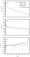 |
Fig. 1. Comparison of the initial profiles of the initial MESA model for the primary star (blue) and the modified models with ideal-gas (yellow) and OPAL (red) equations of state before the relaxation. The gray area indicates the region inside the cut-off radius rcut. The density ρ is shown in panel a (the density profile of the MESA model is hidden behind that of the ideal-gas and OPAL model). The green dots are averaged values of cells in the OPAL model after the relaxation. The specific internal energy u is shown in panel b. The difference between the temperature gradient ∇ and the adiabatic gradient ∇ad is shown in panel c. |
With a resolution of 40 cells per cut-off radius, the maximum Mach numbers inside the star are about 1.0 and 0.1 for the OPAL and ideal-gas EoS, respectively. The deviations from the initial density (and pressure) distribution are small inside the relevant part of the model star’s envelope; the material expanding beyond the initial radius comprises about 1% of the stellar mass. The mass-averaged mean difference of both sides of the hydrostatic equilibrium equation (|ρg − ∇p|/max(|ρg|,|∇p|)) is about 2% for the OPAL model and about 1% for the ideal-gas model. The deviations of the total energy during the relaxation are on the order of a few percent with a maximum in the potential energy of the OPAL model of 3%.
The envelope of the giant is convectively unstable in the MESA model. Mass-averaged mean Mach numbers on the grid after mapping and relaxation are about 0.01 for the ideal-gas models and 0.10 for the OPAL models. These flows are attributed to convection. We reconstruct the mechanical model with its density and pressure profiles. With the same EoS, the thermal structure of the original MESA model is retained, but when changing the EoS, it is not necessarily reproduced. This behavior is illustrated by the superadiabaticity ∇ − ∇ad in Fig. 1c. For the model with the ideal-gas EoS, the mean deviation in the mapped temperature gradient from that of an adiabatic stratification, (∇−∇ad) ∼ − 0.05, is negative in the stellar interior. Thus, we do not expect convection. In contrast, in the model with the OPAL EoS, we obtain (∇−∇ad) ∼ 0. Convection is expected and can indeed be observed to develop in our relaxation simulations (Fig. 2).
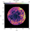 |
Fig. 2. Mach number of the flow at the end of the relaxation of the OPAL model. Cells are larger at larger radii since densities are lower. The region outside the star (ρ < 10−9 g cm−3) is blacked out. |
We calculate the structural parameter λ (Webbink 1984; de Kool et al. 1987) of the AGB star models. The binding energy can be approximated by
 (1)
(1)
where the total mass of the giant star M1 equals the sum of the core and envelope masses, M1 = Mc + Me. In the integral in Eq. (1), we are following Dewi & Tauris (2000) when including the fraction αth (Han et al. 1995) of the internal energy. Using the right-hand side of Eq. (1), we calculate two different values of λ: λg for αth = 0 and λb for αth = 1 (Table 1). Without the internal energy, λg ≈ 0.32 for the OPAL EoS and λg ≈ 0.31 for the ideal-gas EoS. This is consistent with De Marco et al. (2011), whose fit gives λ = 0.28 ± 0.03 for a 1.0 M⊙ AGB star. An additional factor of 1/2 in their definition of λ, however, leads to a systematic offset of −22% compared to our values of λ. Including the internal energy, the envelope is less tightly bound, λb ≈ 2.83 for the OPAL EoS and λb ≈ 0.60 for the ideal-gas EoS.
Envelope structure parameter λ for the 1.0 M⊙ primary.
2.5. Binary setup
We use the initial stellar models discussed above to set up our binary-evolution simulations of the hydrodynamics of CE phases. The relaxed model is placed into a box large enough for the expelled matter not to leave the simulation domain during the runtime (a box size of 1.1 × 10⁵ R⊙ is chosen). The AGB primary star model is placed into a binary system with a less massive companion star of mass M2, which could be a main-sequence star or a white dwarf. Here, we consider mass ratios q = M2/M1 of 0.25, 0.5 and 0.75. The companion star is represented by a point mass. To properly resolve the region around point masses (i.e., the core of the AGB star and the secondary star), we prescribe a spatial resolution of 40 cells per cut-off radius (Sect. 2.4). The gravitational force of the gas particles and point masses is smoothed at a length of h ≈ 1.6 × 10⁻² R⊙ and h ≈ 3.1 R⊙, respectively, following the spline function given in Springel (2010).
The Roche-lobe radius RL of a binary-star system of mass ratio q and orbital separation a is approximately (Eggleton 1983)
 (2)
(2)
Mass transfer starts when the primary AGB star fills its Roche lobe. Subsequently, the orbital separation is expected to shrink and the primary’s radius to increase. Since we cannot follow this initially slow process in our hydrodynamic simulations, we artificially reduce the initial orbital separation, ai, to 60% of the separation for which the AGB star would overflow its Roche lobe (i.e., ai = 0.6 R/rL), assuming RL ≈ R, the primary star’s radius.
In the resulting binary configuration, the companion star is well above the surface of the primary (cf. Table 2). The companion is set up rotating with the orbital period given by Kepler’s law, ![Mathematical equation: $ P = 2 \pi\, [G(M_1+M_2)/a_i^3]^{-1/2} $](/articles/aa/full_html/2020/12/aa38992-20/aa38992-20-eq3.gif) . We set up solid body rotation of the AGB star envelope with 95% of the angular frequency of co-rotation with the companion to facilitate the inspiral.
. We set up solid body rotation of the AGB star envelope with 95% of the angular frequency of co-rotation with the companion to facilitate the inspiral.
Setups for binary runs with mean number of cells N, mass ratio q, initial orbital separations ai and initial orbital periods P.
The initial orbital separations of the CE simulations with the different mass ratios depend on the mass ratio q. This has little effect on the initial orbital energy Eorb and the amount of orbital energy used to eject envelope material, ΔEorb, is mostly determined by the final orbital separation, af. A list of all models presented in this paper and their respective parameters is given in Table 2.
3. Common-envelope simulations
We present the results of the binary simulations: in Sect. 3.1, we start by comparing in detail two reference runs with q = 0.5 for the ideal-gas and the OPAL EoS. Mass unbinding is analyzed in Sect. 3.2 and recombination-energy usage in Sect. 3.3. We discuss the results for different companion masses in Sect. 3.4, the final-to-initial-separation ratio in Sect. 3.5, and the α-formalism in Sect. 3.6.
3.1. Reference runs
A first CEE simulation with q = 0.5 is conducted for both the OPAL-EoS (O.50) and the ideal-gas (I.50) models. The total energy of the systems, defined as the sum of the potential, kinetic and internal energies of the cores (respective primary star core and companion) and the envelopes, is still negative: −0.6 × 1046 erg for the OPAL-EoS and −1.8 × 1046 erg for the ideal-gas model. Therefore, the envelopes of both systems can become entirely unbound only by the additional release of orbital energy. We run the O.50 (I.50) model for about 2500 d (2000 d), amounting to 1.3 × 10⁶ (1.1 × 10⁶) time-step integrations. We follow about 60.4 (70.0) binary orbits, of which 51.2 (56.1) are after the end of the plunge-in, where we define the plunge-in phase as |ȧP|/a > 0.01, in contrast to Ivanova & Nandez (2016) who require |ȧP|/a ≳ 0.1). In Fig. 3, we show the orbital evolution of model O.50.
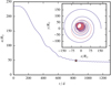 |
Fig. 3. Orbital evolution of the O.50 reference run. The oscillations are due to eccentricity in the inspiral, the star symbol marks the end of the plunge-in phase. In the inset we show the trajectory of the primary in red and that of the secondary star in blue. |
In Fig. 4, we show the evolution of density and Mach number of the OPAL reference run in the orbital (x–y) plane (similar evolution for the ideal-gas EoS). The O.50 (I.50) run starts with an initial orbital period of 346 d (347 d) in the left panels of Fig. 4; the dynamical timescale of the envelope is 30 d and the acoustic timescale is 72 d. The secondary star is enclosed in the common envelope after about 68 d. The cores are surrounded by overdense material and compress material by moving through the now common envelope, forming two spiral arms moving outward. The orbital frequency increases during the inspiral, and, after one orbit, shear instabilities arise within the spiral arms (middle panels of Fig. 4); best visible in the Mach number plot in the lower row). The spiral arms themselves also move outward with higher velocities than previously so that subsequent shock layers hit previous layers. The second arm collides with the first after about 1.6 orbits (400 d) at a distance of about 700 R⊙ from the center of mass. After four orbits (600 d, right panels in Fig. 4), the radius at which consecutive layers hit each other has shrunk to about 200 R⊙ and instabilities form inside this radius where the density is decreased due to the expansion of the AGB primary star.
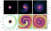 |
Fig. 4. Density and Mach number of model O.50 in the orbital plane at the beginning of the simulation, after one and after four orbits. The core of the primary star is marked by a plus symbol (+) and the secondary star by a cross symbol (×). The regions between the supersonic shocks are transonic, outside of the spiral structure it is supersonic due to the rotation in the setup, the low density and the pressure. |
In the case of the O.50 (I.50) run, 840 d (766 d) after the start of the plunge-in, this phase is terminated at an orbital separation of 50 R⊙ (41 R⊙) and period 39 d (29 d). The slower inspiral in case of the OPAL-EoS run is probably due to the expansion of the envelope accelerated by the release of recombination energy. At the end of the run, after 2500 d (2000 d), the remaining orbital separation has reduced to 41 R⊙ (34 R⊙) and the period is 31 d (23 d). The final orbit has a low eccentricity of e ≈ 0.038 (≈0.010). We measure the eccentricity with the technique proposed by Ohlmann et al. (2016a) by fitting ellipses. At the end of the ideal-gas run, the mass ejection has stagnated; in case of the OPAL EoS, it is still going on. Although increasingly affected by the instabilities, the spiral pattern can still be recognized at late times (Fig. 5), where – as visible in the inset – the two cores still create new shock waves and maintain the spiral structure. We summarize the orbital evolution of the ideal-gas and OPAL-EoS runs for the total run and the plunge-in phase separately in Table 3.
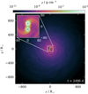 |
Fig. 5. Density in the orbital plane of O.50 at the end of the run. The preserved spiral structure from the inspiral is visible. The core of the primary is marked by a plus symbol (+) and that of the secondary by a cross symbol (×). |
Orbital evolution with different companions.
The angular momentum of the cores as well as their kinetic energy are continuously transferred to the envelope during the plunge-in phase. The transfer of energy of the cores to the envelope mainly acts via the (tidal) drag force in close vicinity of the cores. The error on the angular momentum increases with simulation time to a maximum of 1.1% (1.3%) at the end of the simulation using the OPAL (ideal-gas) EoS.
3.2. Unbound mass
Orbital energy transferred from the cores to the envelope is only one contribution to the overall process powering mass ejection, in particular in case of the OPAL EoS. In fact, it is chiefly the thermal and internal energies of the envelope itself that are converted into kinetic energy (see Table 4). This becomes evident in particular after the plunge-in, when the orbital separation approaches its final value in the simulations. The error in the total energy at the end of plunge-in phase is only 2.0%. Unfortunately, after 2500 d (ΔEtot = 1.91 × 1045 erg, equivalent to a gain of 5.3% of the initial potential energy), the energy error rate of 1.0 × 1037 ergs−1 is larger than the recombination-energy-release rate in the O.50 run and we can no longer reasonably decide whether material becomes unbound or not. We thus choose t = 2500 d as the end of the reference run. We finish the I.50 run after 2000 d with ΔEtot = 0.76 × 1045 erg, that is a gain of 2.1% of the initial potential energy.
Fractions of unbound mass, fej = Mej/Me, and energies for the different companions at the end of the runs.
The unbound mass is defined as the sum of the masses of cells having a positive energy. It is not readily clear how different forms of energy can contribute to the unbinding and we thus consider different criteria (Table 4): fej, kin is the fraction of the envelope mass unbound when only accounting for kinetic energy to balance gravitational binding energy, fej, therm is the fraction unbound when comparing the potential energy of the material to the sum of its kinetic and thermal energies, and fej, OPAL is the fraction unbound when accounting for kinetic plus total internal (thermal and recombination) energy in case of the OPAL EoS. The save conservative definition is to regard as unbound only material for which the kinetic energy exceeds its gravitational potential energy. Ultimately, however, thermal energy will be converted into kinetic energy and also recombination energy may increase it. Because the total energy error in the simulations exceeds the recombination-energy release at late times, we cannot follow the recombination until the unbound mass fraction saturates in our OPAL-EoS based simulations. Instead, we determine the unbound mass fraction by including the recombination energy still stored in the gas in the criterion fej, OPAL. If energy errors could be avoided, this is what our simulations are bound to arrive at. Of course, there is the possibility that energy is lost by radiation before the envelope is completely removed. This effect is currently not accounted for in our modeling (see Sect. 3.3).
For the two reference runs, the unbound mass fractions are plotted versus time in Fig. 6. For I.50, it saturates at about 20% and we can follow the conversion of thermal energy, while in O.50 almost the entire mass is unbound when accounting for the stored internal (ionization) energy. Here, recombination occurs as matter from the envelope cools down when expanding. This leads to further unbinding of material on longer timescales. Most of the recombination energy is only released at rather late times, see Fig. 6. Still, not the entire conversion can be followed in our simulation. We reach 86% unbound mass after 2500 d when accounting for kinetic energy alone and the unbound mass according to this criterion is still increasing when we terminate our simulation. After the plunge-in, about 10% of the envelope’s mass is still inside the orbit of the two cores, but the final mass fraction within the orbit of the two cores, finorb, is only about 2%. Unless there is a change in the overall structure of the remaining envelope, no further dynamical spiral-in is possible due to the low ambient density and the co-rotation of the material leading to a small relative velocity and a vanishing drag force. We discuss the possible fate of the system in Sect. 4.
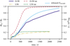 |
Fig. 6. Fraction of ejected mass, Mej, over time for the O.50 (dark blue and red) and the I.50 (yellow and green line) models. It is plotted with kinetic energy only (dark blue and yellow line) and including internal energy (red and green line), respectively, for I.50 (where internal means thermal energy) and O.50 (where internal means thermal plus recombination energy), respectively. The released recombination energy is shown in light blue on the right-hand axis. |
3.3. Recombination energy
We observe similar dynamics for the ideal-gas and OPAL runs, but the ejected mass is larger when including recombination energy. Ions recombine once the envelope has cooled and expanded sufficiently. The released recombination energy can lead to further mass unbinding even after the plunge-in phase has terminated. Because no radiation transport is implemented in our simulations, all of the released recombination energy is thermalized and absorbed locally. This may overestimate the unbound mass, because some radiation may escape in low opacity regions and would therefore not be available to help unbind mass.
In Fig. 7, we show in a time series the remaining recombination energy and an approximation of the position of the photosphere. The latter is determined by integrating the optical depth τ along the x, y and z directions from outside in until reaching τ = 1. Regions inside the spiral structure (between the layers) have a lower remaining ionization energy (see Fig. 7), meaning energy has been released by recombination. This indicates that recombination acts behind the spiral shocks where the gas cools, boosting the expansion.
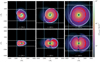 |
Fig. 7. Available ionization energy of Model O.50 in the orbital plane at the beginning of the simulation, after one and after four orbits. The white and light blue lines represent projections of the photosphere along the axes (i.e., they outline the opaque region). The red, green and dark blue contours enclose regions with ionization fractions of H, HeI, and HeII larger than 0.2, respectively. |
Regions with an ionization fraction of > 0.2 for H, HeI and HeII are indicated by isocontours. The remaining recombination energy is mainly inside the photosphere. The approximated photosphere encloses the region up to an ionization fraction of about 0.1 for hydrogen. This suggests that most of the recombination energy is released inside the photosphere such that it can thermalize quickly and thus be used for unbinding the envelope. At the times shown in Fig. 7, 0.9%, 2.4% and 6.1%, respectively, of the recombination energy is outside of the photosphere and thus cannot be completely used for envelope unbinding. It is, however, about 20% at the end of the simulation (2500 d). Comparing the initially available recombination energy (1.2 × 1046 erg, Sect. 2.3) to the recombination energy released by then (0.95 × 1046 erg, Table 4), we note that this share may not be needed to achieve full envelope ejection.
Dust is expected to form at the end of the plunge-in (Iaconi et al. 2020), which would significantly increase the opacity of the material. One requirement for condensation and formation of dust is a temperature below about 2000 K (Nozawa & Kozasa 2013). At the times specified in Fig. 7 (296 d, 600 d and 1000 d), the innermost cell with a temperature below 2000 K is at distance of 1350 R⊙, 2350 R⊙ and 3875 R⊙ to the center, that is about the radius of the photosphere, with densities up to 2 × 10⁻¹³ g cm−3. After 2500 d, it is 8500 R⊙. The condensation radius according to Glanz & Perets (2018) for 1500 K (effective temperature  for our AGB model) is 586 R⊙. After 2500day, about 6% of the envelope mass are still bound each inside and outside this condensation radius measured by the kinetic energy criterion. Because the background temperature on our grid is 1870 K, we cannot follow gas down to the 1500 K assumed by Glanz & Perets (2018). The condensation radius for 2000 K, however, is 329 R⊙, much smaller than the radius of 8500 R⊙ we found after 2500 d. Even when ignoring dust formation, most of the recombination energy is released in optically thick regions, but potential dust formation further supports our assumption that at least large parts of the recombination energy can be used for envelope ejection at late times.
3.4. Different companion stars
We now compare CE simulations of binary systems with the same AGB primary star as before, but mass ratios between the two interacting stars of q= 0.25, 0.5 and 0.75. The key parameters of the orbital evolution in the different runs are summarized in Table 3.
For the ideal-gas EoS, a more massive companion leads to a slower plunge-in, while there is no such clear trend for the OPAL-EoS runs (see values for tpi in Table 3). In terms of release of orbital energy, however, the ideal gas and OPAL-EoS runs are qualitatively similar (see Fig. 8). In case of O.25, the energy release is delayed but higher values from 1300 d on (corresponding to 36.4 [O.25], 22.3 [O.50] and 12.6 [O.75] orbits). Considering the total run, less massive companions spiral in deeper (Podsiadlowski 2001) and release more orbital energy (when measured at the same time; see Table 4). This trend is not unexpected: according to Paczyński (1976), the drag force is weaker for a lower secondary mass, thus transfer of orbital energy to the envelope is less efficient and a deeper inspiral is possible. We find that the spiral-in is deeper by 17%–23% when not including recombination energy compared to the final separations in the simulations that include recombination energy. This can be explained by the fact that without recombination energy release the expansion of the envelope is slower and the transfer of orbital energy terminates later when little mass is within the orbit of the cores. The eccentricity of the orbit is larger for more massive companions because the inspiral is quicker; vice-versa, it is smaller for less massive companions where more orbits are required to reach the final separation and thus the motion circularizes.
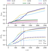 |
Fig. 8. Ejected mass and energy budget for different companions. In the upper panel, the unbound mass fraction over time accounting for kinetic energy only is shown. Dark blue, yellow and light blue lines (OPAL EoS), red, green and purple lines (ideal-gas EoS) are for q = 0.25, q = 0.5 and q = 0.75, respectively. In the lower panel, the released internal (continuous) and orbital energies (dashed lines) are plotted as fractions of the gravitational binding energy for the OPAL runs. The vertical dotted lines indicate tpi from Table 3. |
In Table 4, we compare the unbound mass fractions for different energy contributions with different companions at the end of the runs. For the OPAL EoS, less massive companions can unbind more of the envelope’s mass until the end of the run, but all fractions are still increasing at that time (Fig. 8). For the ideal-gas EoS, the unbound mass fraction has saturated when the simulations are terminated. For the OPAL-EoS runs, the release of orbital energy stagnates and the release rate of internal energy decreases at about tpi, leading to a change of slope in the curve of the unbound mass fraction (Fig. 8). Our criterion for the plunge-in phase, |ȧP|/a > 0.01, captures the instant of slope change accurately for O.25 and O.50; however, the change of slope is not very pronounced in case of O.75 and therefore the criterion is not precise.
The different amounts of released orbital and internal energy due to the slower and deeper inspiral explain the trend in the unbound mass: at the same elapsed physical time, the system with the smallest mass ratio has expelled the largest fraction of envelope material. However, as the mass unbinding still continues by the end of our simulations, this is a statement about the efficiency of mass ejection rather than its overall success. We observe a stronger dynamical response of the envelope for higher companion masses. This leads to rapid expansion and therefore the transfer of orbital energy from the companion onto the envelope gas by tidal drag is less efficient. For very low companion masses, however, the dynamical response may eventually become so weak that the envelope expands only little and insufficient recombination energy is released for envelope ejection (see Kramer et al. 2020). We therefore anticipate an optimal envelope removal efficiency at intermediate mass ratios. Extrapolating from our data, we expect complete envelope ejection in all considered cases. It will be achieved 7.4 yr (O.25), 8.2 yr (O.50) and 9.4 yr (O.75) after the beginning of the simulation.
3.5. Final-to-initial-separation ratio
The ratio of the final to the initial orbital separation given by the formalism in Eq. (4) of Dewi & Tauris (2000) is
 (3)
(3)
A fit of this relation to the data of our OPAL EoS-based simulations with αλ = 2.1 is shown in Fig. 9. Surprisingly, however, a linear relation seems to fit the simulation data better. We perform a linear regression on the ratio of the orbital separations depending on q, the initial mass ratio at the onset of the CE, and find for the OPAL-EoS runs
 (4)
(4)
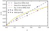 |
Fig. 9. Final orbital configuration as a function of q. Linear fits (dashed lines) to the three data points per EoS (stars) are shown in blue (OPAL EoS) and red (ideal-gas EoS). A fit to Eq. (3) with αλ = 2.1 is shown in yellow. |
whereas we obtain
 (5)
(5)
for the ideal-gas EoS runs. A comparison run with q = 0.5 and a larger initial separation (p = 0.8) was performed, leading to a ratio of af/ai = 48 R⊙/314 R⊙ = 0.15. This is in the range of our fit and confirms that it works well also for different initial separations.
3.6. α-formalism
For the OPAL-EoS runs, we anticipate that the entire envelope is ejected such that we can employ the α-formalism of Webbink (1984). In population synthesis models, the envelope-ejection efficiency αCE of CE phases is usually parametrized in terms of the released orbital energy ΔEorb and the binding energy of the envelope of the primary star Ebin,
 (6)
(6)
This parametrization serves for determining the final orbital separations of compact binary systems formed in CEE. The binding energy Ebin is usually described using the structural parameter λ (see Sect. 2.4). The released orbital energy is approximately given by
![Mathematical equation: $$ \begin{aligned} \Delta E_{\rm orb} \approx - G \left[ \frac{M_c M_2}{2 a_f} - \frac{(M_c + M_e)M_2}{2 a_i} \right], \end{aligned} $$](/articles/aa/full_html/2020/12/aa38992-20/aa38992-20-eq11.gif) (7)
(7)
and thus
![Mathematical equation: $$ \begin{aligned} - G \frac{M_e \left( \frac{1}{2}M_e + M_c \right) }{\lambda R} \approx - \alpha _{\rm CE} G \left[ \frac{M_c M_2}{2 a_f} - \frac{(M_c + M_e)M_2}{2 a_i} \right]. \end{aligned} $$](/articles/aa/full_html/2020/12/aa38992-20/aa38992-20-eq12.gif) (8)
(8)
With an ad-hoc choice of αCE a value for af can be determined.
Our simulations allow to directly determine a value α = Ebin/ΔEorb. We choose the definition of α as in Eq. (6) so that we are as close as possible to population-synthesis models. Therefore, α primarily serves to determine the final orbital separations and has – in this form – little significance for the envelope ejection. The resulting values for α are calculated either using the potential energy only or using the potential and the entire internal energy (i.e., Eg and Eb from Table 1). They are given in Table 5. When only accounting for the gravitational energy, the ejection seems to need more energy than taken from the orbit (αg > 1), but when taking into account also the internal energy, the efficiency αb is less than one. Since we assume complete envelope ejection, computing α is meaningful only for the OPAL-EoS models.
4. Discussion
Previous high-resolution three-dimensional simulations with AREPO by Ohlmann et al. (2016a), conducted with a 2 M⊙ RG star as primary, observe shear instabilities between the individual layers of the spiral structure characteristic for CE interaction. In their simulations, the instability-driven flow patterns grow in size and eventually large-scale flow instabilities wash out the spiral structure completely. Our simulations including the release of recombination energy, however, show no large-scale flow instabilities, only small-scale instabilities arise within the spiral arms. The spiral structure is preserved until large parts of the envelope are ejected. We interpret this effect as a suppression of the instabilities due to a stronger expansion of the envelope gas.
In our simulations without recombination energy, only up to about 20% of the envelope material is expelled. A comparison with the mere 8% mass loss in the simulation of Ohlmann et al. (2016a) with a RG primary star (but an otherwise identical numerical approach) confirms the expected effect of a more efficient envelope ejection for a less tightly bound AGB primary. Differences in the setup of the models, the numerical methods, and the achieved numerical resolutions render a quantitative comparison with other studies difficult. Nonetheless, the 23–31% envelope ejection found by Sandquist et al. (1998) in simulations with more massive AGB primaries of 3 M⊙ and 5 M⊙ and the 25% of unbound envelope mass with an AGB primary of 3.05 M⊙ (3.5 M⊙ ZAMS mass) reported by Staff et al. (2016) fall into the same ballpark.
Chamandy et al. (2020) follow CEE in a simulation with an AGB primary star for 20 orbital revolutions and find an envelope ejection of about 11%. By the end of their simulation, however, the unbound mass is still increasing. They extrapolate that a complete envelope ejection is possible in less than ten years, provided the mass loss rate does not change significantly. Our simulation I.50 (which, like that of Chamandy et al. 2020, ignores recombination energy release) follows the evolution up to 70 orbits. By then, the mass loss rate has decreased substantially. The unbound mass still grows slightly, but with a decreasing rate. It seems questionable if an ejection of more than ∼25% of the envelope mass is possible. The reason for the strong decrease in mass loss after the plunge-in phase is an expansion of envelope gas so that little material is left inside the orbit of the stellar cores. This makes the transfer of orbital energy to the gas inefficient. We cannot, however, exclude the establishment of a self-regulated inspiral phase (Meyer & Meyer-Hofmeister 1979; Podsiadlowski 2001), where the envelope contracts on a thermal time scale and episodes of more efficient energy transfer followed by another phase of expansion and contraction lead to a slow loss of the envelope.
As for the case of CEE with RG primary stars (Nandez et al. 2015; Prust & Chang 2019; Reichardt et al. 2020), the question of accounting for the release of recombination energy turns out to be decisive for the success of envelope ejection also with AGB primaries. Our simulations strongly indicate that a complete envelope removal is possible provided this energy is indeed transferred to the envelope material. Contrary to Grichener et al. (2018), Ivanova (2018) argues that only a negligible fraction of recombination energy is radiated away and most of it can be used to eject the envelope. This is supported by our simulations, where we find that during the evolution most of the remaining ionization energy is located in regions of high optical depths.
Fragos et al. (2019) simulated the complete evolution of a binary system with a 12 M⊙ red supergiant primary star using a 1D hydrodynamic MESA model. Including recombination energy, they conclude that most of the envelope is unbound. However, as in our case, the thermal energy contribution is more important than recombination. Ricker et al. (2019) studied CEE with 82.1 M⊙ red supergiant stars with and without radiative transfer in 3D for the first time and found that for these specific objects recombination energy does not help in envelope removal. This is no contradiction to our result as the structures of the primary stars in the considered mass ranges are quite different (see, e.g., Fig. 5 in Kruckow et al. 2016).
Outflow and unbinding of envelope gas driven by recombination continue after the plunge-in phase in our case. Other mechanisms, such as pre-plunge-in ejection and ejection triggered by a contraction of the circum-binary envelope (Ivanova & Nandez 2016), accretion onto the companion, and dust formation are not necessarily required for successful envelope ejection, but may still play a role. The mass loss rate at the end of our simulations with the OPAL EoS is stable over many orbits. A simple extrapolation yields complete envelope removal within about ten years. The similarity to the value estimated by Chamandy et al. (2020) is probably sheer coincidence, because the physical effects responsible for envelope ejection are different in the models: Chamandy et al. (2020) do not account for recombination effects and extrapolate the mass unbinding found in the initial plunge-in phase.
In our simulations, the core system approaches a final and steady orbital separation. The orbital evolution is similar in the runs accounting for the release of ionization energy and those ignoring this effect. It is largely determined by the initial plunge-in phase. Later recombination processes occur primarily in the outer parts of the envelope and are important for mass ejection, but have less (although not negligible) effect on the inner core binary. Being a key quantity for the future evolution of the eventually formed close compact binary system, we attempt to determine how the final core separation depends on parameters of the initial setup. Remarkably, our simulations suggest a linear relation between the final-to-initial-separation ratio and the mass ratio in the original binary. However, there is no such simple linear relation between the eccentricity and the mass ratio. We provide values for α from our simulations employing the OPAL EoS. We find agreement when comparing our values from the OPAL simulations resulting in λα values of 0.96, 1.06, and 1.46 to the range of 0.75–1.27 reported by Nandez & Ivanova (2016). As discussed by Iaconi & De Marco (2019), our values for the final separations and α are upper limits. In contrast to the hypothesis of Iaconi & De Marco (2019) and Reichardt et al. (2020), however, the final separations determined in our simulation are systematically larger when ionization effects are accounted for. This is explained by the fact that recombination energy is already released during the inspiral and the resulting envelope expansion stalls the orbital shrinking earlier.
The mass ratios q considered in our study have been chosen without referring to a particular model of CE initialization thus raising the question of whether the corresponding systems would enter CEE in the first place. Ge et al. (2010, 2015, 2020a) use an adiabatic mass-loss model to systematically determine critical q values for mass transfer to proceed on a dynamical timescale. They assume conservation of mass and orbital angular momentum, and neglect stellar winds. Ge et al. (2020b) conclude that q = 3/4 may be close to the threshold beyond which stable mass transfer is expected instead of a CE episode for a star like ours. This indicates that our study covers the relevant range in q. The outcome of their CEE with a 3.2 M⊙ AGB primary star (Fig. 7 of Ge et al. 2010) appears similar to a binary system with a 12 M⊙ red supergiant primary star as shown in Fig. 4 of Fragos et al. (2019).
The final orbital separations determined from observations of post-CE binaries show a significant scatter, and deriving the initial system parameters is challenging and introduces uncertainties. Although our simulation results are close to some observed systems (see Iaconi & De Marco 2019), the general tendency in those seems to point toward smaller af than obtained here. This certainly warrants further study. In particular, higher-mass AGB primary stars are expected to lead to a deeper inspiral of the companion because more envelope material has to be ejected.
The final core separations are smaller for lower mass ratios in the AGB systems studied by Sandquist et al. (1998). Our results confirm this trend. Starting at a core distance of 124 R⊙ in a system with mass ratio q = 0.55, Chamandy et al. (2020) find a final separation of 16 R⊙. The resulting af/ai = 0.13 is close to our fit for the ideal-gas runs, even though further spiral-in is probable. Staff et al. (2016) find no convergence with resolution when comparing their runs “4” and “4h”, but their separation ratio falls below our fit.
Our results raise the question of the final fate of the simulated systems. The unbound mass fraction is larger for smaller q by the end of the respective simulations, but it is still increasing in all OPAL runs. We cannot follow the evolution for longer with confidence with our current numerical methods, because the energy-error rate exceeds the recombination-energy-release rate in the system and we can no longer decide whether a further envelope unbinding is physical or caused by numerical errors. Moreover, additional physical effects may become important in the late phases of the evolution modeled here. With further envelope expansion, recombination may not proceed in optically thick regions and the energy may be radiated away instead of aiding mass ejection. A counteracting effect would be the above-mentioned dust formation that may revive energy transfer to envelope material. If the envelope ejection remains incomplete, recurrent CE episodes seem possible until full removal of the material is achieved. In this case, the orbital separation may again shrink (although probably not by much since the binding energy of the remaining material is low) and this would affect its relation to the initial mass ratio and the α values determined here.
5. Conclusions
We present simulations of common envelope interactions of a low-mass AGB primary star (1.2 M⊙ ZAMS mass; 173 R⊙ radius at onset of common-envelope evolution) with different companions using the AREPO code. Our simulations follow the common-envelope evolution up to about 100 orbits of the core binary.
Despite the lower binding energy of the AGB star compared to a RG, envelope ejection stalls below 20% of its mass when not accounting for ionization energy release. By employing the OPAL EoS, we include this effect in our simulations, effectively assuming that the recombination energy liberated in the expanding envelope is thermalized locally. In this case, our simulations indicate that complete envelope ejection is possible.
Comparing simulations with different companion masses, we find that less massive companions spiral in deeper into the envelope. By the time our simulations terminate, they have led to a more complete envelope ejection in our simulations accounting for ionization effects. However, because the unbound mass fraction keeps increasing almost linearly in our simulations including ionization effects, the final envelope ejection is expected to be complete in all cases under the assumption of local thermalization of released recombination energy. Because of the stronger dynamical response of the envelope for more massive companions and the lack of expansion and recombination energy release for too low-mass companions, we expect an optimal envelope removal efficiency at intermediate mass ratios of the two stars.
At least in the important early phases recombination energy is released in optically thick regions, such that it cannot be radiated away and is bound to support mass loss. This supports the assumptions made in our simulations. For a final verdict on envelope ejection, however, a proper treatment of the release of energy from recombination processes and the associated radiation requires the inclusion of radiative transfer.
Our simulations indicate that a simple linear relation may provide a satisfactory fit to the dependence of the final orbital separation of the core binary on the initial mass ratio between secondary and primary star. This has to be confirmed with further simulations exploring a wider parameter space.
Acknowledgments
The work of C. S. and F. K. R. was supported by the Klaus Tschira Foundation. Parts of this work were performed on the computational resource ForHLR I funded by the Ministry of Science, Research and the Arts Baden-Württemberg and DFG (“Deutsche Forschungsgemeinschaft”). For data processing and plotting, NumPy (Oliphant 2006) and SciPy (Virtanen et al. 2020), IPython (Pérez & Granger 2007), and Matplotlib (Hunter 2007) were used. We thank the anonymous referee, Noam Soker and Matthias Kruckow for helpful comments.
References
- Belczynski, K., Kalogera, V., & Bulik, T. 2002, ApJ, 572, 407 [NASA ADS] [CrossRef] [Google Scholar]
- Bermúdez-Bustamante, L. C., García-Segura, G., Steffen, W., & Sabin, L. 2020, MNRAS, 493, 2606 [NASA ADS] [CrossRef] [Google Scholar]
- Biermann, L. 1938, ZAp, 16, 29 [Google Scholar]
- Blöcker, T. 1995, A&A, 297, 727 [NASA ADS] [Google Scholar]
- Chamandy, L., Frank, A., Blackman, E. G., et al. 2018, MNRAS, 480, 1898 [NASA ADS] [CrossRef] [Google Scholar]
- Chamandy, L., Blackman, E. G., Frank, A., Carroll-Nellenback, J., & Tu, Y. 2020, MNRAS, [Google Scholar]
- de Kool, M. 1990, ApJ, 358, 189 [NASA ADS] [CrossRef] [Google Scholar]
- de Kool, M., van den Heuvel, E. P. J., & Pylyser, E. 1987, A&A, 183, 47 [NASA ADS] [Google Scholar]
- De Marco, O., Passy, J.-C., Moe, M., et al. 2011, MNRAS, 411, 2277 [NASA ADS] [CrossRef] [Google Scholar]
- Dewi, J. D. M., & Tauris, T. M. 2000, A&A, 360, 1043 [NASA ADS] [Google Scholar]
- Eggleton, P. P. 1983, ApJ, 268, 368 [NASA ADS] [CrossRef] [Google Scholar]
- Fragos, T., Andrews, J. J., Ramirez-Ruiz, E., et al. 2019, ApJ, 883, L45 [NASA ADS] [CrossRef] [Google Scholar]
- Ge, H., Hjellming, M. S., Webbink, R. F., Chen, X., & Han, Z. 2010, ApJ, 717, 724 [NASA ADS] [CrossRef] [Google Scholar]
- Ge, H., Webbink, R. F., Chen, X., & Han, Z. 2015, ApJ, 812, 40 [NASA ADS] [CrossRef] [Google Scholar]
- Ge, H., Webbink, R. F., Chen, X., & Han, Z. 2020a, ApJ, 899, 132 [CrossRef] [Google Scholar]
- Ge, H., Webbink, R. F., & Han, Z. 2020b, ApJS, 249, 9 [CrossRef] [Google Scholar]
- Glanz, H., & Perets, H. B. 2018, MNRAS, 478, L12 [NASA ADS] [CrossRef] [Google Scholar]
- Górski, K. M., Hivon, E., Banday, A. J., et al. 2005, ApJ, 622, 759 [NASA ADS] [CrossRef] [Google Scholar]
- Grichener, A., Sabach, E., & Soker, N. 2018, MNRAS, 478, 1818 [CrossRef] [Google Scholar]
- Han, Z., Podsiadlowski, P., & Eggleton, P. P. 1994, MNRAS, 270, 121 [NASA ADS] [CrossRef] [Google Scholar]
- Han, Z., Podsiadlowski, P., & Eggleton, P. P. 1995, MNRAS, 272, 800 [Google Scholar]
- Hillwig, T. C., Jones, D., De Marco, O., et al. 2016, ApJ, 832, 125 [NASA ADS] [CrossRef] [Google Scholar]
- Hunter, J. D. 2007, Comput. Sci. Eng., 9, 90 [NASA ADS] [CrossRef] [Google Scholar]
- Iaconi, R., & De Marco, O. 2019, MNRAS, 490, 2550 [CrossRef] [Google Scholar]
- Iaconi, R., Reichardt, T., Staff, J., et al. 2017, MNRAS, 464, 4028 [NASA ADS] [CrossRef] [Google Scholar]
- Iaconi, R., Maeda, K., Nozawa, T., De Marco, O., & Reichardt, T. 2020, MNRAS, 497, 3166 [CrossRef] [Google Scholar]
- Iben, I., Jr, & Tutukov, A. V. 1984, ApJS, 54, 335 [NASA ADS] [CrossRef] [Google Scholar]
- Ivanova, N. 2018, ApJ, 858, L24 [NASA ADS] [CrossRef] [Google Scholar]
- Ivanova, N., & Nandez, J. L. A. 2016, MNRAS, 462, 362 [NASA ADS] [CrossRef] [Google Scholar]
- Ivanova, N., Justham, S., Chen, X., et al. 2013, A&ARv, 21, 59 [Google Scholar]
- Izzard, R. G., Hall, P. D., Tauris, T. M., & Tout, C. A. 2012, IAU Symp., 283, 95 [Google Scholar]
- Kalogera, V., & Webbink, R. F. 1998, ApJ, 493, 351 [NASA ADS] [CrossRef] [Google Scholar]
- Kramer, M., Schneider, F. R. N., Ohlmann, S. T., et al. 2020, A&A, 642, A97 [CrossRef] [EDP Sciences] [Google Scholar]
- Kruckow, M. U., Tauris, T. M., Langer, N., et al. 2016, A&A, 596, A58 [NASA ADS] [CrossRef] [EDP Sciences] [Google Scholar]
- Kuruwita, R. L., Staff, J., & De Marco, O. 2016, MNRAS, 461, 486 [CrossRef] [Google Scholar]
- Livio, M., & Soker, N. 1988, ApJ, 329, 764 [NASA ADS] [CrossRef] [Google Scholar]
- Livio, M., Shankar, A., Burkert, A., & Truran, J. W. 1990, ApJ, 356, 250 [NASA ADS] [CrossRef] [Google Scholar]
- Meyer, F., & Meyer-Hofmeister, E. 1979, A&A, 78, 167 [NASA ADS] [Google Scholar]
- Nandez, J. L. A., & Ivanova, N. 2016, MNRAS, 460, 3992 [NASA ADS] [CrossRef] [Google Scholar]
- Nandez, J. L. A., Ivanova, N., & Lombardi, J. C. 2015, MNRAS, 450, L39 [NASA ADS] [CrossRef] [Google Scholar]
- Nordhaus, J., Blackman, E. G., & Frank, A. 2007, MNRAS, 376, 599 [NASA ADS] [CrossRef] [Google Scholar]
- Nozawa, T., & Kozasa, T. 2013, ApJ, 776, 24 [NASA ADS] [CrossRef] [Google Scholar]
- Ohlmann, S. T., Röpke, F. K., Pakmor, R., & Springel, V. 2016a, ApJ, 816, L9 [NASA ADS] [CrossRef] [Google Scholar]
- Ohlmann, S. T., Röpke, F. K., Pakmor, R., Springel, V., & Müller, E. 2016b, MNRAS, 462, L121 [NASA ADS] [CrossRef] [Google Scholar]
- Ohlmann, S. T., Röpke, F. K., Pakmor, R., & Springel, V. 2017, A&A, 599, A5 [NASA ADS] [CrossRef] [EDP Sciences] [Google Scholar]
- Oliphant, T. E. 2006, A guide to NumPy, 1 (USA: Trelgol Publishing) [Google Scholar]
- Paczyński, B. 1976, in Structure and Evolution of Close Binary Sytems, eds. P. Eggleton, S. Mitton, & J. Whelan, IAU Symp., 73, 75 [CrossRef] [Google Scholar]
- Paczyński, B., & Ziółkowski, J. 1968, Acta Astron., 18, 255 [Google Scholar]
- Pakmor, R., Kromer, M., Röpke, F. K., et al. 2010, Nature, 463, 61 [NASA ADS] [CrossRef] [PubMed] [Google Scholar]
- Passy, J.-C., De Marco, O., Fryer, C. L., et al. 2012, ApJ, 744, 52 [NASA ADS] [CrossRef] [Google Scholar]
- Paxton, B., Bildsten, L., Dotter, A., et al. 2011, ApJS, 192, 3 [Google Scholar]
- Paxton, B., Cantiello, M., Arras, P., et al. 2013, ApJS, 208, 4 [NASA ADS] [CrossRef] [Google Scholar]
- Paxton, B., Marchant, P., Schwab, J., et al. 2015, ApJS, 220, 15 [Google Scholar]
- Pérez, F., & Granger, B. E. 2007, Comput. Sci. Eng., 9, 21 [Google Scholar]
- Podsiadlowski, P. 2001, in Evolution of Binary and Multiple Star Systems, eds. P. Podsiadlowski, S. Rappaport, A. R. King, F. D’Antona, & L. Burderi, ASP Conf. Ser., 229, 239 [NASA ADS] [Google Scholar]
- Prust, L. J., & Chang, P. 2019, MNRAS, 486, 5809 [CrossRef] [Google Scholar]
- Rasio, F. A., & Livio, M. 1996, ApJ, 471, 366 [NASA ADS] [CrossRef] [Google Scholar]
- Reichardt, T. A., De Marco, O., Iaconi, R., Chamandy, L., & Price, D. J. 2020, MNRAS, 494, 5333 [CrossRef] [Google Scholar]
- Reimers, D. 1975, Mem. Soc. Roy. Liège, 8, 369 [Google Scholar]
- Ricker, P. M., & Taam, R. E. 2012, ApJ, 746, 74 [NASA ADS] [CrossRef] [Google Scholar]
- Ricker, P. M., Timmes, F. X., Taam, R. E., & Webbink, R. F. 2019, in IAU Symposium, eds. L. M. Oskinova, E. Bozzo, T. Bulik, & D. R. Gies, 346, 449 [Google Scholar]
- Rogers, F. J., & Nayfonov, A. 2002, ApJ, 576, 1064 [Google Scholar]
- Rogers, F. J., Swenson, F. J., & Iglesias, C. A. 1996, ApJ, 456, 902 [NASA ADS] [CrossRef] [Google Scholar]
- Ruiter, A. J., Belczynski, K., & Fryer, C. 2009, ApJ, 699, 2026 [NASA ADS] [CrossRef] [Google Scholar]
- Ruiter, A. J., Sim, S. A., Pakmor, R., et al. 2013, MNRAS, 429, 1425 [NASA ADS] [CrossRef] [Google Scholar]
- Sabach, E., Hillel, S., Schreier, R., & Soker, N. 2017, MNRAS, 472, 4361 [NASA ADS] [CrossRef] [Google Scholar]
- Sandquist, E. L., Taam, R. E., Chen, X., Bodenheimer, P., & Burkert, A. 1998, ApJ, 500, 909 [NASA ADS] [CrossRef] [Google Scholar]
- Sandquist, E. L., Taam, R. E., & Burkert, A. 2000, ApJ, 533, 984 [NASA ADS] [CrossRef] [Google Scholar]
- Shiber, S., Iaconi, R., De Marco, O., & Soker, N. 2019, MNRAS, 488, 5615 [CrossRef] [Google Scholar]
- Soker, N., Grichener, A., & Sabach, E. 2018, ApJ, 863, L14 [NASA ADS] [CrossRef] [Google Scholar]
- Springel, V. 2010, MNRAS, 401, 791 [NASA ADS] [CrossRef] [Google Scholar]
- Staff, J. E., De Marco, O., Macdonald, D., et al. 2016, MNRAS, 455, 3511 [NASA ADS] [CrossRef] [Google Scholar]
- Taam, R. E., & Ricker, P. M. 2010, New Astron. Rev., 54, 65 [NASA ADS] [CrossRef] [Google Scholar]
- Taam, R. E., & Sandquist, E. L. 2000, ARA&A, 38, 113 [NASA ADS] [CrossRef] [Google Scholar]
- Terman, J. L., Taam, R. E., & Hernquist, L. 1994, ApJ, 422, 729 [CrossRef] [Google Scholar]
- Toonen, S., Nelemans, G., & Portegies Zwart, S. 2012, A&A, 546, A70 [NASA ADS] [CrossRef] [EDP Sciences] [Google Scholar]
- Virtanen, P., Gommers, R., Oliphant, T. E., et al. 2020, Nat. Methods [Google Scholar]
- Webbink, R. F. 1984, ApJ, 277, 355 [NASA ADS] [CrossRef] [Google Scholar]
- Wilson, E. C., & Nordhaus, J. 2019, MNRAS, 485, 4492 [CrossRef] [Google Scholar]
- Wilson, E. C., & Nordhaus, J. 2020, MNRAS, 497, 1895 [CrossRef] [Google Scholar]
All Tables
Setups for binary runs with mean number of cells N, mass ratio q, initial orbital separations ai and initial orbital periods P.
Fractions of unbound mass, fej = Mej/Me, and energies for the different companions at the end of the runs.
All Figures
|
Fig. 1. Comparison of the initial profiles of the initial MESA model for the primary star (blue) and the modified models with ideal-gas (yellow) and OPAL (red) equations of state before the relaxation. The gray area indicates the region inside the cut-off radius rcut. The density ρ is shown in panel a (the density profile of the MESA model is hidden behind that of the ideal-gas and OPAL model). The green dots are averaged values of cells in the OPAL model after the relaxation. The specific internal energy u is shown in panel b. The difference between the temperature gradient ∇ and the adiabatic gradient ∇ad is shown in panel c. |
| In the text | |
|
Fig. 2. Mach number of the flow at the end of the relaxation of the OPAL model. Cells are larger at larger radii since densities are lower. The region outside the star (ρ < 10−9 g cm−3) is blacked out. |
| In the text | |
|
Fig. 3. Orbital evolution of the O.50 reference run. The oscillations are due to eccentricity in the inspiral, the star symbol marks the end of the plunge-in phase. In the inset we show the trajectory of the primary in red and that of the secondary star in blue. |
| In the text | |
|
Fig. 4. Density and Mach number of model O.50 in the orbital plane at the beginning of the simulation, after one and after four orbits. The core of the primary star is marked by a plus symbol (+) and the secondary star by a cross symbol (×). The regions between the supersonic shocks are transonic, outside of the spiral structure it is supersonic due to the rotation in the setup, the low density and the pressure. |
| In the text | |
|
Fig. 5. Density in the orbital plane of O.50 at the end of the run. The preserved spiral structure from the inspiral is visible. The core of the primary is marked by a plus symbol (+) and that of the secondary by a cross symbol (×). |
| In the text | |
|
Fig. 6. Fraction of ejected mass, Mej, over time for the O.50 (dark blue and red) and the I.50 (yellow and green line) models. It is plotted with kinetic energy only (dark blue and yellow line) and including internal energy (red and green line), respectively, for I.50 (where internal means thermal energy) and O.50 (where internal means thermal plus recombination energy), respectively. The released recombination energy is shown in light blue on the right-hand axis. |
| In the text | |
|
Fig. 7. Available ionization energy of Model O.50 in the orbital plane at the beginning of the simulation, after one and after four orbits. The white and light blue lines represent projections of the photosphere along the axes (i.e., they outline the opaque region). The red, green and dark blue contours enclose regions with ionization fractions of H, HeI, and HeII larger than 0.2, respectively. |
| In the text | |
|
Fig. 8. Ejected mass and energy budget for different companions. In the upper panel, the unbound mass fraction over time accounting for kinetic energy only is shown. Dark blue, yellow and light blue lines (OPAL EoS), red, green and purple lines (ideal-gas EoS) are for q = 0.25, q = 0.5 and q = 0.75, respectively. In the lower panel, the released internal (continuous) and orbital energies (dashed lines) are plotted as fractions of the gravitational binding energy for the OPAL runs. The vertical dotted lines indicate tpi from Table 3. |
| In the text | |
|
Fig. 9. Final orbital configuration as a function of q. Linear fits (dashed lines) to the three data points per EoS (stars) are shown in blue (OPAL EoS) and red (ideal-gas EoS). A fit to Eq. (3) with αλ = 2.1 is shown in yellow. |
| In the text | |
Current usage metrics show cumulative count of Article Views (full-text article views including HTML views, PDF and ePub downloads, according to the available data) and Abstracts Views on Vision4Press platform.
Data correspond to usage on the plateform after 2015. The current usage metrics is available 48-96 hours after online publication and is updated daily on week days.
Initial download of the metrics may take a while.