| Issue |
A&A
Volume 683, March 2024
|
|
|---|---|---|
| Article Number | A65 | |
| Number of page(s) | 17 | |
| Section | Stellar structure and evolution | |
| DOI | https://doi.org/10.1051/0004-6361/202347397 | |
| Published online | 06 March 2024 | |
Going from 3D to 1D: A 1D approach to common-envelope evolution
1
Heidelberger Institut für Theoretische Studien, Schloss-Wolfsbrunnenweg 35, 69118 Heidelberg, Germany
e-mail: This email address is being protected from spambots. You need JavaScript enabled to view it.
2
Zentrum für Astronomie der Universität Heidelberg, Astronomisches Rechen-Institut, Mönchhofstr. 12-14, 69120 Heidelberg, Germany
3
University of Oxford, St Edmund Hall, Oxford OX1 4AR, UK
4
Zentrum für Astronomie der Universität Heidelberg, Institut für Theoretische Astrophysik, Philosophenweg 12, 69120 Heidelberg, Germany
Received:
7
July
2023
Accepted:
1
November
2023
Abstract
The common-envelope (CE) phase is a crucial stage in binary star evolution because the orbital separation can shrink drastically while ejecting the envelope of a giant star. Three-dimensional (3D) hydrodynamic simulations of CE evolution are indispensable to learning about the mechanisms that play a role during the CE phase. While these simulations offer great insight, they are computationally expensive. We propose a one-dimensional (1D) model to simulate the CE phase within the stellar-evolution code MESA by using a parametric drag force prescription for dynamical drag and adding the released orbital energy as heat into the envelope. We computed CE events of a 0.97 M⊙ asymptotic giant branch star and a point-mass companion with mass ratios of 0.25, 0.50, and 0.75, and compared them to 3D simulations of the same setup. The 1D CE model contains two free parameters, which we demonstrate are both needed to fit the spiral-in behavior and the fraction of ejected envelope mass of the 1D method to the 3D simulations. For mass ratios of 0.25 and 0.50, we find well-fitting 1D simulations, while for a mass ratio of 0.75, we do not find a satisfactory fit to the 3D simulation as some of the assumptions in the 1D method are no longer valid. In all our simulations, we find that the released recombination energy is needed to accelerate the envelope and drive the ejection.
Key words: hydrodynamics / methods: numerical / stars: AGB and post-AGB / binaries: close / stars: mass-loss
© The Authors 2024
 Open Access article, published by EDP Sciences, under the terms of the Creative Commons Attribution License (https://creativecommons.org/licenses/by/4.0), which permits unrestricted use, distribution, and reproduction in any medium, provided the original work is properly cited.
This article is published in open access under the Subscribe to Open model. This email address is being protected from spambots. You need JavaScript enabled to view it. to support open access publication.
1. Introduction
Common-envelope (CE) evolution, originally proposed by Paczyński (1976), is a phase in binary star evolution during which a giant star engulfs its more compact companion, leading to the formation of a shared envelope around the core of the giant star and the companion. Frictional forces cause the binary orbit to shrink. The released orbital energy expands the envelope, which can result in complete or partial envelope ejection while forming a close binary or a merger of the two stars if the envelope cannot be fully ejected (for reviews, see Ivanova et al. 2013; De Marco & Izzard 2017; Röpke & De Marco 2023). Today, it is believed that CE evolution is the main mechanism for converting wide binary star systems into close binaries (Ivanova et al. 2013). Therefore, CE evolution plays an important, often essential role in our understanding of the formation channels of close binary systems, such as the CE channel for gravitational-wave sources (Tutukov & Yungelson 1993; Belczynski et al. 2002; Voss & Tauris 2003; Eldridge & Stanway 2016; Stevenson et al. 2017; Kruckow et al. 2018; Vigna-Gómez et al. 2018; Spera et al. 2019; for a more complete summary of references, see, e.g., Mandel & Broekgaarden 2022), possibly the progenitors of type Ia supernovae (Iben & Tutukov 1984; Webbink 1984; Whelan & Iben 1973), X-ray binaries (Tauris & van den Heuvel 2006), cataclysmic variables (Warner 1995), short-period hot subdwarfs (Heber 2009), and even potentially gamma-ray burst sources (Fryer & Woosley 1998; Izzard et al. 2004; Detmers et al. 2008.
Soon after CE evolution was proposed, one-dimensional (1D) simulations were carried out by Taam et al. (1978) and Meyer & Meyer-Hofmeister (1979). Using 1D hydrodynamic simulations, Podsiadlowski (2001) found that the CE evolution can be divided into distinct phases. During the “initial phase”, the co-rotation between the binary star and the envelope of the giant star is lost. Frictional forces then lead to the rapid spiral-in of the binary star during the “plunge-in phase”, which is the shortest phase during CE evolution, happening on the dynamical timescale of the binary. As the CE expands, the spiral-in slows down, which might then lead to the “self-regulated spiral-in phase”, its “termination”, and the “post-CE evolution”, during which the changes in the orbital separation are small compared to the plunge-in phase (see Ivanova et al. 2013 for the definitions of the final stages). In this study, we followed the approach of Röpke & De Marco (2023) and combined all stages after the plunge-in phase into the “post-plunge-in phase”.
Three dimensional (3D) (magneto)hydrodynamic simulations of CE events (Ricker & Taam 2008, 2012; Passy et al. 2012; Nandez et al. 2014; Ohlmann et al. 2016a,b; Iaconi et al. 2017; Chamandy et al. 2018; Prust & Chang 2019; Reichardt et al. 2019; Sand et al. 2020; Ondratschek et al. 2022; Lau et al. 2022a,b; Moreno et al. 2022) are currently the best tool for studying the physical mechanisms that cause the spiral-in of the binary and the ejection of the envelope. These simulations are computationally expensive and easily need more than 105 core-hours. They allow us to study CE events case by case, but they are infeasible when studying larger populations of systems undergoing CE evolution.
An energy formalism was introduced to predict the outcome of a CE event (Webbink 1984; Livio & Soker 1988): the released orbital energy is compared to the binding energy of the envelope, where the CE efficiency, αCE, determines the fraction of the orbital energy that is used to unbind the envelope. Classically, an efficiency of αCE ≤ 1 is assumed to account for energy conservation. However, energy sources other than the orbital energy might be available, for example the ionization energy from the recombination of hydrogen and helium (Han et al. 1995; Ivanova et al. 2015), accretion on the companion (Chamandy et al. 2018), the formation of jets (Shiber et al. 2019), and dust formation (Glanz & Perets 2018; Iaconi et al. 2020; Reichardt et al. 2020). These extra energy sources allow physical scenarios with αCE > 1. Therefore, the energy formalism cannot be used directly by itself to predict the outcome of a CE event, since the efficiency parameter, αCE, varies from system to system (Iaconi & De Marco 2019). Recent efforts have been made by Marchant et al. (2021) and Hirai & Mandel (2022) to improve on the energy formalism.
Even though 3D simulations are constantly improving and more computational power is available, 1D simulations of the CE phase remain a useful tool (cf. Ivanova & Nandez 2016; Clayton et al. 2017; Fragos et al. 2019; Trani et al. 2022). The comparatively low computational costs of 1D simulations compared to 3D simulations open the opportunity to study a larger number of CE systems and explore the possible parameter space (Ivanova et al. 2013). This makes 1D simulations more versatile than 3D simulations. Semi-analytic models calibrated on 3D simulations (e.g., Trani et al. 2022) have similar advantages.
As outlined above, it is still a difficult task to predict the outcome of CE events, because the input physics of 1D methods is incomplete, prohibiting accurate simulations of CE evolution, while 3D simulations are computationally too expensive. In this paper we introduce a new 1D method for efficiently computing CE events. The assumptions made in 1D models, such as spherical symmetry and energy deposition in shells, do not capture the physical processes involved in CE events. To compensate for this, we introduced free parameters, which we calibrated on the characteristics of 3D simulations (e.g., the orbital separation and the mass of the ejected envelope). We tested to see how many parameters are needed for the 1D simulation to reproduce the characteristics of 3D simulations. Our method needs to be calibrated on 3D simulations to obtain the most accurate results while still retaining the computational advantages of a 1D simulation. If possible, the calibrated method can be used to simulate CE events and predict their outcome.
This paper is structured as follows. In Sect. 2 we describe our new 1D CE method. Then, we apply this method to simulate CE events of a 0.97 M⊙ asymptotic giant branch (AGB) star and point-mass companions. Detailed results of the simulation with a mass ratio of 0.25 are shown in Sect. 3, and the results for simulations with mass ratios of 0.50 and 0.75 are presented in Sect. 4. Finally, we discuss our proposed model and the results in Sect. 5, and conclude in Sect. 6.
2. Methods
We modeled the 3D CE simulation of Sand et al. (2020) in the 1D stellar-evolution MESA revision 12778 (Paxton et al. 2011, 2013, 2015, 2018, 2019). We describe how to obtain the same pre-CE giant star as Sand et al. (2020) in Sect. 2.1 and our general hydro setup in Sect. 2.2. For numerical reasons, we first performed a relaxation run of the pre-CE model, which we explain in Sect. 2.3. Frictional forces are hindering the motion of the companion inside the envelope and cause the orbit to decay. In Sect. 2.4, we introduce a parametric prescription of this drag force and show how the drag force modifies the equations of motion that we integrated to obtain the binary orbit. The mass of the companion modifies the gravitational potential of the giant star, which we describe in Sect. 2.5. In Sect. 2.6, we show how we modeled the back reaction of the companion on the envelope by artificially heating the envelope layers around the companion. The unbound layers at the surface of the CE are removed from the simulation, as explained in Sect. 2.7. Within this model, we used two calibration parameters; one parameter determines the strength of the drag force, and the other sets the size of the artificially heated zone. In Sect. 2.8 we show how we calibrate these parameters by comparing our 1D simulations to 3D hydrodynamic simulations of CE events of Sand et al. (2020).
2.1. Initial model
We evolved an initially 1.2 M⊙ star with metallicity Z = 0.02 from the zero-age main sequence to the AGB phase and stop the evolution once the model reaches a mass of 0.97 M⊙. For this run, we used the default MESA settings, except for changing the wind-loss parameters in the Reimers prescription to ηR = 0.5 (Reimers 1975) and in the Blöcker prescription to ηB = 0.1 (Blöcker 1995). Additionally, we disabled the MESA “gold tolerances” to evolve the model through the helium flash, and we used a mixing-length parameter of αMLT = 2.
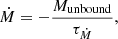
Our initial model of the AGB star has a radius of 166 R⊙. This is similar to the radius of 172 R⊙ for the initial model of Sand et al. (2020). The density in the envelope of our initial model is ∼5 − 10% higher compared to the initial model for the 3D simulations (Fig. 1), with deviations of up to 45% close to the surface. We attribute this to the older MESA revision 7624 used to construct the initial pre-CE model in Sand et al. (2020), which makes it difficult to reproduce the exact same model.
 |
Fig. 1. Initial density profile ρini, 1D of the AGB star in comparison to the initial density profile ρini, 3D of the AGB star in Sand et al. (2020), as well as the 1D and 3D density profiles after the relaxation run, ρrelax, 1D and ρrelax, 3D. Relative deviations between the density profiles are shown along the secondary ordinate. |
2.2. Hydrodynamic setup in MESA
We simulated the CE evolution in MESA using its single star module star together with an artificial heating source to account for the presence of a companion star. We switched to the implicit hydrodynamics in MESA by using the Harten-Lax-van Leer-Contact (HLLC; Toro et al. 1994) approximate Riemann solver (Paxton et al. 2018). With implicit hydrodynamics, we can study the dynamical evolution of the CE and also capture potential shocks. To better resolve shocks near the surface of the envelope, we imposed a vanishing compression gradient for the surface boundary condition that sets the surface density (Paxton et al. 2015; Grott et al. 2005). For the other surface boundary condition, here the temperature, we used a black body.
We used an adaptive mesh refinement in the velocity, optimized for hydrodynamic simulations in MESA (Paxton et al. 2018), with uniform spacing in log r for the cells. The number of cells was chosen to be similar to the number of cells in the initial hydrostatic model. As this mesh refinement does not support rotation of the star, we simulated the CE without accounting for rotation in the stellar structure equations.
The hydrodynamic equations with MESA’s HLLC scheme are solved implicitly in time. Thus, the timesteps of our simulations are not limited by the Courant-Friedrichs-Lewy (CFL) criterion (Courant et al. 1928; Paxton et al. 2018). However, to resolve shock waves that travel through the envelope, we limited the timesteps to 45% of the maximum timestep given by the CFL criterion. Furthermore, we find that limiting the timesteps to < 10−4 yr helps with the numerical stability of the simulations. All the 1D CE simulations were run for as long as possible and stop for numerical reasons, for example too short timesteps.
2.3. Relaxation run
Before starting the CE simulation, we performed a relaxation, where we switched from the standard hydrostatic solver to the implicit hydrodynamic solver and changed the surface boundary conditions. The relaxation run lasted for 2 yr, or about 15 dynamical timescales1. During the final 0.2 yr of the relaxation run, the maximum timestep was linearly decreased to a value of 10−7 yr. We find that this helps start the CE simulation from the relaxed model without numerical artifacts.
During the relaxation run, the envelope expands to 189 R⊙. The density profile of the envelope of the AGB star changes by less than 5% during the relaxation run (Fig. 1). At the end of the relaxation run, the density close to the surface of the star decreased by 60%. This shows that mostly the surface layers of the star expand during the relaxation run, leaving the envelope structure unchanged. Figure 1 also compares the density profile after the relaxation run to the relaxed density profile of Sand et al. (2020). Throughout most parts of the envelope, the density profiles deviate by less than 10%, except for larger deviations toward the surface. The deviations toward smaller radii originate from the cut-out core in the 3D simulation.
2.4. Orbital evolution
We integrated the equations of motion of the classical two-body problem consisting of an extended sphere at location x1, representing the giant star, and a point-mass particle at location x2, representing the companion, to compute the orbital evolution of the binary star. In general, quantities with index 1 refer to the giant star, while index 2 refers to the companion. As the companion is revolving within the giant star during the CE event, only the mass of the giant star enclosed by the orbit M1, aorb needs to be considered in the equations of motion,
 (1)
(1)
 (2)
(2)
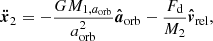
where the orbital separation (i.e., the distance from the center of the giant star to the point-mass companion) is given by aorb = x2 − x1. The mass of the companion is given by M2 and G is the gravitational constant. Vector quantities in non-bold notation denote the absolute value of that quantity and  is a unit vector in the direction of x. Because the companion moves within the envelope of the giant star, it is subject to a drag force
  caused by dynamical friction, opposing the relative velocity vrel of the companion to the envelope.
We used the semi-analytic formalism of Kim (2010) and Kim & Kim (2007) to calculate the drag force. Kim & Kim (2007) extended the classical model of dynamical friction of Ostriker (1999) to perturbers moving in circular orbits with radius r through a homogeneous background medium of density ρ. Kim (2010) then extended the model further to account for possible nonlinear effects arising from the circular motion of the perturber. They define the two dimensionless parameters
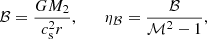 (3)
(3)
with M2 the mass of the perturber (i.e., the companion in our case), cs the sound speed, and ℳ = vrel/cs the Mach number. They find a correction term fρ for the density to account for nonlinear effects,
 (4)
(4)
Together, the drag force is then given by
![Mathematical equation: $$ \begin{aligned} F_\mathrm{d} = {\left\{ \begin{array}{ll} {C_\mathrm{d} } \dfrac{4 \pi \rho _\mathrm{nl} {(G M_2)}^2}{v_\mathrm{rel} ^2} \left( \dfrac{0.7}{\eta _\mathcal{B} ^{0.5}} \right) \quad&\mathrm{for} \ \ \ \eta _\mathcal{B} > 0.1 \wedge \mathcal{M} > 1.01, \\ [1em] {C_\mathrm{d} } \dfrac{4 \pi \rho {(G M_2)}^2}{v_\mathrm{rel} ^2} I&\mathrm{else} , \end{array}\right.} \end{aligned} $$](/articles/aa/full_html/2024/03/aa47397-23/aa47397-23-eq7.gif) (5)
(5)
where the condition ηB > 0.1 and ℳ > 1.01 corresponds to a regime in which nonlinear effects are present that modify the drag force, as opposed to the classical linear regime for ηℬ < 0.1 or ℳ < 1.01. The drag-force parameter Cd is introduced as a free parameter in our model and modifies the strength of the drag force. We modified the original condition by Kim (2010) for the nonlinear regime from ℳ > 1 to ℳ > 1.01 in Eq. (5) to avoid divergence issues in the definitions of ηℬ and ρnl. According to Kim & Kim (2007), the Coulomb logarithm I in the linear regime is given by
![Mathematical equation: $$ \begin{aligned} I = {\left\{ \begin{array}{ll} 0.7706 \ln \left(\dfrac{1 + \mathcal{M} }{1.0004 - 0.9185\, \mathcal{M} } \right) - 1.473\, \mathcal{M} \quad \mathrm{for} \ \ \mathcal{M} < 1.0, \\ [1em] \ln \left(330 \dfrac{r}{r_\mathrm{min} } \dfrac{(\mathcal{M} - 0.71)^{5.72}}{\mathcal{M} ^{9.58}}\right) \quad \mathrm{for} \ \ 1.0 \le \mathcal{M} < 4.4, \\ [1em] \ln \left( \dfrac{r / r_\mathrm{min} }{0.11\,\mathcal{M} + 1.65}\right) \quad \mathrm{for} \ \ 4.4 \le \mathcal{M} . \end{array}\right.} \end{aligned} $$](/articles/aa/full_html/2024/03/aa47397-23/aa47397-23-eq8.gif) (6)
(6)
We chose rmin = 3.1 R⊙, a measure of the size of the companion, which is the same value as the softening-length of the gravitational potential of the companion in the simulations of Sand et al. (2020).
The initial orbital separation aorb, ini in Sand et al. (2020) was chosen such that the giant star overfills its Roche lobe, initiating the CE event. In particular, the companion is initially outside of the giant star (i.e., aorb, ini > R1). This setup of the initial orbit would not lead to a CE event in our 1D model on a dynamical timescale, because the companion does not exert a tidal force on the giant star. Additionally, we assumed a vanishing density around the giant star, which leads to a vanishing drag force and no spiral-in behavior. Therefore, to initiate the CE event, we chose aorb, ini = 160 R⊙; that is to say, we placed the companion well inside the giant’s envelope of 166 R⊙ before the relaxation. The initial orbit is set up to be circular, following the setup in Sand et al. (2020).
The giant star in the simulations of Sand et al. (2020) is initially set up to rotate rigidly at 95% of the initial orbital frequency with the angular velocity vector Ω pointing perpendicular to the orbital plane. We used the same Ω for our 1D simulations as in Sand et al. (2020), which means in particular that Ω varies with the mass ratio q = M2/M1.
The relative velocity of the companion to the envelope of the giant star is given by
 (7)
(7)
where vr(aorb) is the (radial) expansion velocity of the CE at the location of the companion. While the giant star in the MESA simulation does not rotate (Sect. 2.2), a rigidly rotating envelope with a constant angular velocity Ω in time is assumed for calculating the relative velocity. The magnitude of the relative velocity enters the calculation of the drag force via Eq. (5).
The equations of motion (Eqs. (1) and (2)) are integrated in parallel with the MESA simulation using a fifth-order explicit Runge-Kutta method with an embedded fourth-order error estimation (Cash & Karp 1990). Relative and absolute error tolerances are set to 10−10, and the maximum integration timestep is set so that at least ten orbit-integration steps are taken during one MESA timestep.
2.5. Modified gravitational potential
For the simulations of the CE evolution with our 1D model, we used the single-star module star of MESA to model the giant star. However, because of the mass of the companion, which is revolving inside the envelope of the giant star, the gravitational potential can no longer be approximated by that of a single star. To account for the change in the gravitational potential, we modified the gravitational constant G to a radius-dependent gravitational constant  with
with
 (8)
(8)
where M1, r is the mass of the giant star within radius r (Podsiadlowski et al. 1992). This ensures that the layers outside the orbit are bound more strongly to the system because of the additional mass of the companion. Layers within the orbit are not affected. Changing the gravitational constant modifies not only the binding energy of the outer layers but also the entire envelope profile, for example density and pressure.
2.6. CE heating
The drag force acting on the companion inside the CE dissipates the orbital energy of the binary system, causing the orbital separation to shrink. The rate at which orbital energy is dissipated is given by Ėdis = Fd · vrel. We added the dissipated energy from the binary orbit by artificially increasing the internal energy of the envelope, that is, heating with the same rate as the orbital energy is lost (i.e., Ėheat = −Ėdis).
The range over which energy is injected is approximated by the accretion radius of the Bondi-Lyttleton-Hoyle accretion model (Hoyle & Lyttleton 1941; Bondi & Hoyle 1944). The accretion radius profile Ra(r) inside the envelope is given by
 (9)
(9)
where Δv(r) is the relative velocity of the spherical shell at coordinate r with respect to the companion, and cs(r) is the sound speed. The relative velocity is given by
 (10)
(10)
where
 (11)
(11)
 (12)
(12)
In the above equations, vorb = ẋ2 − ẋ1 is the orbital velocity and vr(r) is the (radial) expansion velocity of the envelope. The quantities vorb, r and vorb, φ are the projections of the orbital velocity vector along the r direction and the φ direction.
The accretion radius defines the area of influence of the companion in the giant’s envelope. We chose to heat all the envelope layers with a radial coordinate between  and
and  , which are determined by solving
 (13)
(13)
 (14)
(14)
The heating parameter Ch is introduced as a free parameter in our models and determines the extent of the heating zone by modifying the upper and lower boundary for the heating zone via Eqs. (13) and (14). If there are multiple solutions2 for Eqs. (13) and (14), we used the largest one for  and the smallest one for
  (i.e., the solutions closest to aorb). This definition ensures that for all layers with
  , the radial separation from the companion is smaller than the local accretion radius; in other words, these layers are gravitationally deflected and focused behind the companion. The heating rate
  then follows
![Mathematical equation: $$ \begin{aligned} \dot{\epsilon }_\mathrm{heat} \sim {\left\{ \begin{array}{ll} \exp \left[-\left(\dfrac{a_\mathrm{orb} - r}{a_\mathrm{orb} - r^\mathrm{heat} _{\min }}\right)^2 \right] \quad&\mathrm{for} \ r^\mathrm{heat} _{\min } \le r < a_\mathrm{orb} , \\ [1em] \exp \left[-\left(\dfrac{a_\mathrm{orb} - r}{a_\mathrm{orb} - r^\mathrm{heat} _{\max }}\right)^2 \right]&\mathrm{for} \ a_\mathrm{orb} \le r \le r^\mathrm{heat} _{\max },\\ [1em] 0&\mathrm{else} , \end{array}\right.} \end{aligned} $$](/articles/aa/full_html/2024/03/aa47397-23/aa47397-23-eq24.gif) (15)
(15)
which is normalized so that the total heating rate matches the dissipation rate of the orbital energy (i.e.,  ). In the case where
  is undefined by Eq. (14) because r ≠ aorb + Ra(r) for aorb ≤ r ≤ R1, we chose
  . The lower heating limit
  is always well defined because the sound speed increases by orders of magnitude toward the giant’s core, causing the accretion radius to decrease.
2.7. Dynamical envelope ejection
The heating perturbs the hydrostatic equilibrium of the envelope, causing it to expand on the dynamical timescale. Envelope layers exceeding the local escape velocity vesc are formally unbound. The local escape velocity is given by
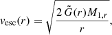 (16)
(16)
where  is the modified gravitational constant defined by Eq. (8). We removed all surface layers with vr > vesc in our CE simulations to avoid numerical difficulties in the unbound layers. If a continuous layer of unbound mass3, Munbound, (i.e., vr > vesc for all shells in this layer) reaches the outer boundary of the simulation domain, we removed the layer exponentially by adopting a mass-loss rate
 (17)
(17)
where τṀ is the mass-loss timescale. In all our simulations, we chose τṀ = 0.01 yr, which is shorter than both the dynamical timescale and the thermal timescale of the envelope. The applied mass-loss prescription is the same as that in Clayton et al. (2017).
2.8. Comparison to 3D CE simulations
We compared and fit our 1D results to those of Sand et al. (2020). In particular, we compared the time evolution of the orbital separation aorb(t), hereafter called the spiral-in curve, and the mass fraction of the ejected envelope, fej,
 (18)
(18)
where Menv = M1 − M1, core is the envelope mass, M1 is the mass of the giant star and M1, core = 0.545 M⊙4. In contrast to this, Sand et al. (2020) defined the total unbound mass, and hence the mass fraction of the ejected envelope, as the sum of all cells with positive total energy (i.e., the sum of the potential and kinetic energy). To better match this quantity, we defined a second envelope-ejection fraction,
 (19)
(19)
 (20)
(20)
where Munbound is the total mass of all layers in the envelope with vr > vesc. The difference between fej and fej, all is that fej, all also includes the layers with vr > vesc within the envelope.
We incorporated two free parameters in our model. The drag-force parameters Cd modifies the strength of the drag force via Eq. (5) and the heating parameter Ch modifies the extent of the heated layers via Eqs. (13) and (14). Both parameters are used to fit the spiral-in curves and the mass fraction of the ejected envelope material from the 1D CE simulations to the results of the corresponding 3D simulations in Sand et al. (2020).
The initial orbital separations of our 1D simulations deviate from the initial separations used by Sand et al. (2020; see Sect. 2.4). Therefore, the spiral-in curve of the 3D simulation is shifted by Δt with respect to the spiral-in curve of the 1D simulation. The optimal time shift Δtmin for fixed Cd and Ch is found by minimizing the mean relative deviation (MRD) between the spiral-in curves,
 (21)
(21)
where T is the total simulated time, δti is the timestep and  are the orbital separations in the 1D and 3D simulation. For the calculation of the MRD, only the plunge-in phase is considered (i.e., the phase during which the orbital separation changes dynamically5). The end of the plunge-in phase is determined by
 (22)
(22)
where the time average is computed over one full orbit. This defines the end of the plunge-in phase when the average change in orbital separation during one orbit is less than 1%. At the beginning of the CE phase in the 3D simulations, a transition of the initially circular orbit toward the dynamical spiral-in is observed. These first 100 d are omitted in the MRD calculations in Eq. (21).
The best fit of the 1D simulation to the 3D simulation is determined manually. We find the best-fitting simulation by computing 1D CE models with varying values for Cd and Ch. For each simulation, we find Δtmin and then compare by eye the spiral-in curve and the mass fraction of ejected envelope to the 3D simulation.
We tested the above described method at different spacial and temporal resolutions and present the results in Appendix A.
3. Results for mass ratio q = 0.25
In this section, we show the results of our 1D CE simulations with mass ratio q = 0.25 and compare our results with the 3D hydrodynamic simulations of Sand et al. (2020). First, we present the best-fitting 1D CE simulations in Sect. 3.1. We then show how the drag-force parameter Cd and the heating parameter Ch affect the outcome of the simulations in Sect. 3.2. In Sect. 3.3, the dynamical processes taking place in the envelope are discussed, before we describe recombination processes in Sect. 3.4. The energy budget during the CE phase and the evolution of the drag force are shown in Sects. 3.5 and 3.6, respectively.
3.1. Best-fitting 1D simulation for q = 0.25
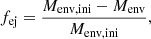
The spiral-in curve of the best-fitting 1D simulation with parameters Cd = 0.23 and Ch = 4.0 for a mass ratio of q = 0.25 is shown in Fig. 2. The spiral-in curve of the 3D benchmark model of Sand et al. (2020) for the same mass ratio is also shown. We find Δtmin = −58 d to best account for the difference in the initial separation (see Sect. 2.8). The plunge-in phase is well reproduced by the 1D simulation. The orbital separation of the 1D simulation after the plunge-in phase is smaller than in the 3D simulation. In both the 1D and the 3D simulations, the post-plunge-in orbit shows a nonzero eccentricity. The eccentricity, e, of the orbit can be approximated as
 (23)
(23)
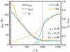 |
Fig. 2. Best-fitting 1D CE simulation for q = 0.25 when comparing to the 3D CE simulation of Sand et al. (2020). Full lines show the orbital separation, and the dotted and dash-dotted lines show the mass fraction of ejected envelope fej and fej, all, respectively. The results of the 3D simulations are shown in orange, and the results from this work are shown in blue. The vertical dashed gray line indicates the end of the dynamical plunge-in phase as determined by Eq. (22). The 3D simulation results are all shifted by Δtmin = −58 d to compensate for the difference in the initial separation. The gray shaded region shows t < 0 d, for which we cannot compare the 1D simulation to the 3D simulation. |
where A is the apastron distance and P is the periastron distance. This approximation is valid as long as the orbital separation is not changing significantly during one orbit, for example during the post-plunge-in phase of the CE evolution. In the 1D simulation, we find an eccentricity of 0.005, which is approximately equal to the eccentricities of 0.006 in the 3D simulation (for a summary, see Table 1). In both cases, the eccentricity is evaluated at the end of the plunge-in phase as determined by Eq. (22), and averaged over five orbits.
Fitting parameters of the three 1D CE simulations.
The fraction of unbound envelope material fej is also shown in Fig. 2. For the 1D simulation, two descriptions (fej and fej, all) are used to determine the fraction of the unbound envelope (Sect. 2.8). In the 3D simulation, the envelope ejection starts at t < 0 d and reaches 0.1 at t = 0 d (Fig. 2). As the companion starts to enter the envelope, it causes one large spiral arm where mass is immediately ejected (Sand et al. 2020). In the 1D simulation, envelope ejection sets in later during the simulations. When considering fej, all, the envelope ejection starts at t = 700 d compared to t = 850 d based on fej. This is expected since fej, all captures all the unbound mass that is considered for fej and, additionally, all layers with vr > vesc inside the envelope. At the end of the 1D simulation, about 70% of the envelope is unbound, and fej ≈ fej, all; in other words, there are only unbound layers at the outer boundary of the CE, not within the CE. It is important to note that the slopes of the fraction of the ejected envelope (i.e., the envelope-ejection rate) at the end of the simulations are similar in both the 1D and 3D case, possibly suggesting a similar ejection mechanism. The envelope ejection in the 1D simulations relies on the energy released from the recombination of hydrogen and helium and will be analyzed in more detail in Sect. 3.3.
The 1D simulation ended because of too short timesteps. However, it seems appropriate to assume that the envelope ejection will be sustained if the simulation is run for longer, possibly leading to a full envelope ejection. At the end of the 3D simulation at 4000 d, 91% of the envelope is ejected (cf. Table 4 in Sand et al. 2020).
Although there are small quantitative differences between the 1D CE simulation in this work and the 3D CE simulations of Sand et al. (2020), it is remarkable that it is possible to achieve such similar results with our 1D model.
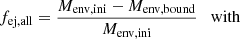
3.2. Role of Cd and Ch for the orbital spiral-in and envelope ejection
In Fig. 3 we show how Cd and Ch affect the orbital separation and the mass fraction of the ejected envelope by varying Cd between 0.1 and 1.0 at the best-fiting Ch (i.e., Ch = 4.00), and by varying Ch between 1.0 and 10.0 at the best-fitting Cd (i.e., Cd = 0.23). For simplicity, we only show fej in Fig. 3. However, we find for all simulations that fej ≈ fej, all during the late phases of the simulations, where the envelope-ejection rate is constant (Figs. 2 and 9).
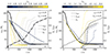 |
Fig. 3. Effects of Cd and Ch on the spiral-in curves, aorb, and the envelope-ejection fraction, fej. In panel a the heating parameter is held constant at Ch = 4.00 and the drag-force parameter, Cd, is varied. In panel b the drag-force parameter is held constant at Cd = 0.23 and the heating parameter, Ch, is varied. The thick black lines in both panels show the results from the 3D hydrodynamic CE simulation of Sand et al. (2020), which are shifted by Δtmin = −58 d, the time shift determined using the best-fitting 1D simulation with Cd = 0.23 and Ch = 4.00. |
The slope of the spiral-in is mostly determined by the strength of the drag force via Cd (Fig. 3a). When varying Cd between 0.1 and 1.0 at fixed Ch, the spiral-in timescale decreases from more than 1500 d to less than 200 d. Additionally, the envelope ejection starts earlier for larger Cd while also ejecting a larger fraction of the envelope. The start of the rapid envelope ejection occurs at similar orbital separations of about 30 R⊙ throughout the different simulations. The post-plunge-in separation changes only slightly when varying the drag-force parameter Cd.
We find that the heating parameter Ch plays an important role in determining the mass fraction of the ejected envelope, but not so much in setting the post-plunge-in separation (Fig. 3b). Increasing the heating parameter causes a slightly deeper spiral-in of the companion and a higher fraction of ejected envelope. The behavior of fej for Cd = 0.23 and varying Ch between 3.2 and 4.2 is noteworthy. In this range, a changing Ch results in a large change in fej while the orbital separation at the end of the plunge-in changes only between 22.9 R⊙ for Ch = 3.2 and 21.3 R⊙ for Ch = 4.2. For the same models, the envelope-ejection curves show a rapid ejection event at the beginning, after which a steadier envelope ejection settles in. In this second phase, the envelope-ejection rates seem to be the same for all the simulations, which are also in agreement with the 3D simulation. This is another indicator that the envelope ejection, especially in the later phase of the simulation, is mainly caused by recombination processes because the recombination rate is comparable between the models (Sect. 3.4). Only the timing and strength of the initial rapid ejection event is changing when varying Ch. Therefore, the heating parameter Ch is important to set the envelope ejection in the 1D CE simulation.
From these experiments, we conclude that the drag-force parameter, Cd, mostly affects the orbital separation during the plunge-in phase by determining the spiral-in timescale. The final mass-fraction of the ejected envelope is determined by both the heating parameter, Ch, and the drag-force parameter, Cd. The orbital separation after the plunge-in phase changes only slightly when varying Cd and Ch. This suggests that there is a more fundamental principle that sets the post-plunge-in separation and that does not depend on the details of the plunge-in-phase. When comparing the 1D model to the 3D simulation, we cannot match the results with only one of the two parameters. Therefore, two parameters are needed in 1D CE models similar to ours to reproduce the spiral-in curve as well as the envelope ejection.
3.3. Dynamical evolution of the envelope
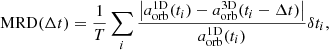
The dynamical evolution of the envelope is shown by several Kippenhahn diagrams in Figs. 4 and 5. During the first ∼200 d, the envelope oscillates radially. These oscillations are artifacts of the change to the hydrodynamic mode in MESA as well as the change in the boundary condition, which are not yet fully damped during the relaxation run (see Sect. 2.3). As the velocities in these oscillations are small compared to the expected expansion velocity, which is comparable to the escape velocity, they do not affect the further evolution of the CE.
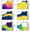 |
Fig. 4. Kippenhahn diagrams of the simulation with q = 0.25, Cd = 0.23, and Ch = 4.0. In panel a, the radial velocity is shown in terms of the local escape velocity; layers colored in red have a radial velocity higher than the local escape velocity. Panels b, c, and d show the ionization fractions of H II, HeII, and He III, respectively. The heating kernel as described in Eq. (15) is shown in panel e, and the specific heating rate in panel f. The red line indicates the orbital separation between the companion and the core of the giant star. The dotted gray region is heated during the CE simulation. The dashed cyan line shows Rτ = 10, which traces the hydrogen-recombination radius. The dashed gray lines represent envelope-mass fractions of 0.95, 0.9, 0.8, 0.6, 0.4, 0.2, 0.1, 0.06, 0.04, and 0.03 from the surface toward the center, and visualize the expansion of the envelope. The white patches in panel a show layers that have an inward (negative) radial velocity. |
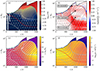 |
Fig. 5. Kippenhahn diagrams (similar to Fig. 4) of the simulation with q = 0.25, Cd = 0.23, and Ch = 4.0, showing the Mach number (ℳ= vr/cs) in panel a, velocity divergence (dv/dr) in panel b, specific entropy (s) in panel c, and opacity (κ) in panel d. The white hatched zones in panel c indicate convective mixing. For a better visualization of the velocity divergence, the log modulus transformation, logmod(x) = sgn(x)log10(|x|+1), is used (John & Draper 1980). The arrows in panel b roughly indicate the recombination zones of H I, He I, and He II (see also Figs. 4b–d). |
After this initial phase, the envelope begins to expand, as more and more heat is injected into the outer layers (see Fig. 7). The partial ionization zones of hydrogen and helium are expanding together with the envelope, as can be seen in Figs. 4b–d, and no recombination is happening yet.
For t < 700 d, we find  , that is, the upper boundary of the heating zone coincides with the outer boundary of the simulation domain. Once
  for t > 700 d, the specific heating rate
  increases by about one order of magnitude because the mass of the material that is heated is decreasing significantly (Figs. 4e,f). As the upper heating radius moves deeper in the envelope, the partial ionization zones of singly ionized hydrogen and helium are no longer heated and recombination sets in. The beginning of recombination and the end of heating in these zones are causally connected, as the heating provides an energy source that keeps the atoms ionized. This is also the reason why Ch determines the ejection of the envelope so strongly.
The layer in which hydrogen recombination takes place moves outward in radius at a typical optical depth of τ = 10 (Rτ = 10), hereafter referred to as the hydrogen-recombination radius, below the outer boundary of the simulation. We find that Rτ = 10 stays always close to the hydrogen recombination front because, above the hydrogen recombination layer, the opacity drops dramatically (Fig. 5d). In fact, this layer expands faster than the local escape velocity (Fig. 4a). This demonstrates that the energy released from hydrogen recombination provides an important acceleration mechanism in expanding and ejecting the envelope. Even though the recombination spatially takes place close to the photosphere (with τ ∼ 1), it is still in the optically thick region where the recombination photons cannot freely escape6 (also see Ivanova & Nandez 2016; Clayton et al. 2017). On top of this fast layer at 700 d ≤ t ≤ 1000 d, there is a slower-moving layer that prevents the fast-expanding layer from becoming unbound and being removed. As the fast material crashes in the slower layer on top, a shock wave is produced, seen by the large negative velocity divergence dv/dr in Fig. 5b.
Layers exceeding vesc reach the outer simulation boundary at t = 1000 d. Then, a rapid mass-loss event removes ∼30% of the envelope mass in a short period of time, followed by continuous steady envelope ejection. The sudden mass-loss event can also be seen in Fig. 2, as the mass fraction of ejected envelope fej increases rapidly at t = 1000 d.
We find that Rτ = 10 stays constant for 700 − 1200 d, after which Rτ = 10 decreases as the hydrogen recombination front moves to smaller radii. At about t = 1400 d, the singly ionized helium-recombination front is located at the hydrogen-recombination radius, which means that hydrogen and singly ionized helium recombine at approximately the same physical location. The released recombination energy accelerates the envelope material, which can be seen by the increase in the slope of the lines of constant mass in Fig. 4.
Along the hydrogen-recombination radius, there is a layer of positive velocity divergence dv/dr (Fig. 5b). This is another indicator that the energy from hydrogen recombination contributes to accelerate the envelope. The recombination of singly and doubly ionized helium also causes layers of positive velocity divergence but with a smaller magnitude compared to the recombination of hydrogen. Because the partial ionization zones of singly and doubly ionized helium are more radially extended than the partial ionization zone of hydrogen, the increase in the velocity divergence is less pronounced. Once the upper heating radius decreases at t = 700 d, the velocity divergence inside the heating zone (i.e., all layers with  ) increases significantly (Fig. 5b). This is an immediate consequence of the increase in the specific heating rate as a result of the decrease in the total envelope mass that is heated (Fig. 4f). Therefore, the localized heating source causes the envelope to expand rapidly. At the same time, there is an outward-traveling feature defined by a lower velocity divergence compared to the surroundings (Fig. 5b). This feature is launched at t = 750 d at the top of the heating zone and reaches the outer boundary at t = 1000 d. The cause of this feature, possibly a pressure/acoustic wave, is likely connected to the decrease in the size of the heating layers.
The neutral layers outside the hydrogen-recombination radius expand supersonically (Fig. 5a). The sound speed of the outer layers is significantly lower due to adiabatic and photon cooling in the neutral layers (Fig. 5c). These outward moving layers show alternating positive and negative velocity divergence (Fig. 5b), that is, there are alternating layers with faster and slower expansion velocities compared to the average expansion velocity of the envelope. The details of the origin of this pattern are unclear. The large negative velocity divergence at the end of the simulation between 200 − 300 R⊙ indicates a shock wave, but we cannot observe any direct consequences arising from the shock.
The white hatching in Fig. 5c shows layers in the CE that are unstable against convection. Initially, the entire envelope is convective, that is, the entropy gradient is less than or equal to zero. Heating stops the convective energy transport after about 200 d, at the same time as the envelope begins to expand. For t < 200 d, the injected energy is transported almost instantaneously to the outer boundary, without affecting the entropy structure of the envelope. As the heating rate increases with time (Fig. 4f) because of the increase in the drag force, the injected energy stops convection. Consequently, the energy cannot be transported away by convection but rather leads to an expansion of the envelope. As energy is injected into the heating zone, the specific entropy in the heating zone increases. The gradient of the heating rate  is positive between
  and aorb (Eq. (15)). Hence, the entropy gradient is also expected to be positive for
  , implying that these layers become stable against convection. While for
  the heating rate decreases (Eq. (15)) and most of these layers are also stable against convection for t > 750 d. They have a positive entropy gradient because the heat/entropy of the inner layers is transported outward. Outside the hydrogen-recombination radius, the transport of energy by radiation is more efficient than convection due to the lower opacity. Some smaller convective zones are visible close to the companion and the outer boundary of the CE at the end stages of the simulations. They are not expected to affect the evolution of the CE because of their limited radial extent.
At the end of the simulation, the opacity close to the outer boundary of the CE increases (Fig. 5f). This increase is caused by the appearance of hydrogen molecules that can form at such low temperatures and densities. At these temperatures, dust formation close to the outer boundary might be possible as well, but it is not included in our simulations (dust formation is expected at a temperature ∼1200 − 2100 K; Iaconi et al. 2020).
3.4. Recombination energy
To study the effects of recombination on envelope ejection, we calculated the amount of released recombination energy. For this, the ionization potentials of hydrogen (H II), singly ionized helium (He II), and doubly ionized helium (He III) are taken from Kramida et al. (2021),
 (24)
(24)
 (25)
(25)
 (26)
(26)
and the atomic masses from Prohaska et al. (2022),
 (27)
(27)
 (28)
(28)
The potentially available energy from the recombination of hydrogen and helium, usually referred to as the recombination energy, is then given by
![Mathematical equation: $$ \begin{aligned}&E_\mathrm{rec} = \int \limits _{M_\mathrm{1,core} }^{M_1}\left[ \frac{X}{m_\mathrm{H} }E_{{\text{ H}}{\small {\uppercase {\text{ ii}}}}} f_{{\text{ H}}{\small {\uppercase {\text{ ii}}}}} \right.\nonumber \\&\qquad \left. + \frac{Y}{m_\mathrm{He} }\Big (E_{{\text{ He}}{\small {\uppercase {\text{ ii}}}}} f_{{\text{ He}}{\small {\uppercase {\text{ ii}}}}} + (E_{{\text{ He}}{\small {\uppercase {\text{ iii}}}}} + E_{{\text{ He}}{\small {\uppercase {\text{ ii}}}}}) f_{{\text{ He}}{\small {\uppercase {\text{ iii}}}}} \Big ) \right]\mathrm{d} m, \end{aligned} $$](/articles/aa/full_html/2024/03/aa47397-23/aa47397-23-eq56.gif) (29)
(29)
where X and Y are the mass fractions of hydrogen and helium, and fH II, fHe II, and fHe III are the ionization fractions of H II, HeII, and HeIII, respectively7. The recombination energies of elements more massive than helium are not taken into account, because their contribution to the total recombination energy is negligible (Ivanova & Nandez 2016).
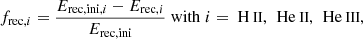
In Fig. 6, we show the fractions frec, total and frec, i of released recombination energy,
 (30)
(30)
 (31)
(31)
 |
Fig. 6. Fraction of released recombination energy (frec) and contributions of hydrogen (H II), singly ionized helium (He II), and doubly ionized helium (He III) for the simulation with q = 0.25, Cd = 0.23, and Ch = 4.0. The total fraction of released recombination energy is shown in black. The horizontal dashed colored lines show the initially available recombination energy in each species. The vertical dashed gray line indicates the end of the dynamical plunge-in phase as determined by Eq. (22). |
where Erec, i is computed by integrating each term in Eq. (29) individually.
The released recombination energy is negligible for t < 700 d. This can be understood with the help of Fig. 5, which shows that the partial ionization zones of hydrogen and helium remain at constant mass coordinates during this time. At the end of the simulation, more than 98% of the initially available recombination energy is released, and about 70% of the released energy is due to hydrogen recombination. The reason for this is the high abundance of hydrogen in the envelope (Xini = 0.7). For 600 d ≤ t ≤ 750 d, we find frec, He II < 0, because doubly ionized helium recombines to form singly ionized helium such that the recombination energy available from singly ionized helium is higher than the initial recombination energy stored in singly ionized helium.
Our calculations show that recombination energy is likely to provide an important contribution to the envelope ejection process. Hydrogen recombination occurs well below the photosphere (at a typical optical depth τ = 10), where photons cannot escape directly. This results in a positive velocity divergence at the location where hydrogen recombines, causing further acceleration of the envelope (Fig. 5b). The recombination front of singly ionized helium is deeper in the envelope compared to the recombination front of hydrogen. Around this recombination zone, the velocity divergence is positive. It is not as large as in the case of hydrogen recombination but much more extended radially. A similar behavior can be observed for the recombination zone of doubly ionized helium. There is a layer of negative velocity divergence around the He III recombination zone for t > 1300 d. As most of the doubly ionized helium has already recombined at this point (see Fig. 6), the energy released might not be enough to further accelerate the envelope.
At the end of the plunge-in phase, about 50% of the available recombination energy is released, while only ∼40% of the envelope is ejected. Hereafter, the energy that drives the envelope ejection is mostly from recombination and no longer from the heating, as by definition the orbital separation decreases slowly in the post-plunge-in phase, which means that the drag force and hence the heating are much lower than during the plunge-in phase (see also Sects. 3.5 and 3.6). At the end of the simulation, more than 70% of the envelope is ejected, which suggests that the recombination energy contributes significantly to the ejection, especially in the post-plunge-in phase. For a comparison, at the end of the 3D simulation at t = 2500 d, 91% of the envelope mass is ejected (Sand et al. 2020).
3.5. Energy budget
Major energy sources and sinks during the 1D CE simulation are shown in Fig. 7. The energies are shown in units of the initial binding energy8 of the envelope,
 (32)
(32)
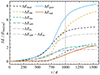 |
Fig. 7. Major energy sources (dashed lines) and sinks (solid lines) during the CE simulation with q = 0.25, Cd = 0.23, and Ch = 4.0. Shown are the total injected energy, ΔEheat, the change in internal energy, ΔEint, the total released recombination energy, ΔErec (the recombination energy is part of the internal energy and is only shown separately to highlight the contribution from recombination), the change in orbital energy, ΔEorb, according to Eq. (34), the extra term ΔEm defined by Yarza et al. (2022), the change in the gravitational energy, ΔEgrav, and the energy that is carried away by radiation, ΔErad. The vertical dashed gray line indicates the end of the dynamical plunge-in phase as determined by Eq. (22). The energies are shown in units of the initial binding energy of the envelope with Ebind, ini = −4.03 × 1045 erg, calculated via Eq. (32). The lines showing contributions from ΔEorb and ΔEm are dash-dotted as they show source terms for the heating ΔEheat but are not direct energy sources in the MESA simulation. |
where u is the internal energy. The total energy injected via heat is determined from the drag force and the relative velocity by
 (33)
(33)
The source of the heating energy is the orbital energy of the two stars in the CE phase. The released orbital energy is classically given by
 (34)
(34)
where M1, aorb is the mass of M1 enclosed by the orbit with separation aorb. From Fig. 7, it is clear that ΔEheat is approximately a factor of 2 larger than −ΔEorb. This discrepancy is expected in our CE formalism because we mix both 1D and 3D treatments of physical mechanisms. For example, we evolved the binary orbit in 3D but were bound to use 1D approximations to calculate the change in potential energy. Therefore, we cannot expect to conserve energy in our CE formalism; in other words, we do expect ΔEheat ≠ −ΔEorb.
In addition, Eq. (34) only applies to systems, where the envelope is completely ejected, and the ejecta has zero velocity at infinity. In our simulations, the abovementioned criteria are not fulfilled, and, therefore, Eq. (34) is insufficient to capture all the relevant effects. This means that there is a need for extra terms in Eq. (34) to correctly calculate ΔEorb in 1D CE treatments similar to ours. One such term arises from the change in potential energy because of the change in the enclosed mass. In the limit M2 ≪ M1, aorb, Yarza et al. (2022) suggest this term to be
 (35)
(35)
where M1, r is the mass of the giant star enclosed by the radius r. We tested the effect of adding the term ΔEm in the calculation of the orbital energy in Eq. (34) for our simulation to see if it can resolve the observed mismatch between ΔEheat and −ΔEorb. Even when considering the contribution of ΔEm to the change in orbital energy, there is more energy injected in the envelope than is released (Fig. 7). We note that in our simulation the condition M2 ≪ M1, aorb is not fulfilled. Further reasons for the discrepancy are that the change in the orbital energy is not only caused by the change in the orbital separation but also by the envelope expansion. As the envelope expands, the mass enclosed by the orbit M1, aorb decreases and thus the potential energy of the companion. This means that the orbital energy of a companion at a constant aorb inside an expanding envelope increases because of the decrease in the enclosed mass by the orbit. This effect is not included in the term ΔEm proposed by Yarza et al. (2022).
Additionally, the energy loss via radiation at the outer boundary of the envelope is shown in Fig. 7 as well as the energy release from the recombination of hydrogen and helium. The losses from radiation are about half of the energy injected via heat. Both the losses via radiation and the energy gain from recombination start to become significant for t > 700 d, after which they increase almost synchronously. This does not mean that the energy released from recombination is immediately radiated away, but rather that it contributes to accelerate the envelope material, for example as shown by the kink in the lines of constant mass at the hydrogen recombination front (Fig. 4b) as well as by the positive velocity divergence (Fig. 5b). This acceleration can even cause the layers to expand faster than the local escape velocity (Fig. 4a).
3.6. Drag force evolution
The drag force acting on the companion is calculated by Eq. (5) following the results of Kim (2010) and Kim & Kim (2007). In Fig. 8, we show the individual components that enter the drag force as well as the ratio of the drag force and the gravitational force Fg. The drag force increases for t < 750 d. From Fig. 8 it is apparent that the drag force is mostly influenced by the density ρ and the relative velocity vrel as they vary the most compared to the other components of the drag force. For t < 750 d, the density increases, which causes the drag force to increase. The relative velocity increases throughout the entire simulation because the orbital velocity increases with  and the rotational velocity decreases with ∼aorb as the orbit separation aorb decreases (compare Eq. (7)). Hence, the drag force, which is proportional to
  , decreases. For t < 750 d, the increase in ρ dominates over the decrease in
  , causing the drag force to increase. For t > 750 d, the drag force decreases, because both the ρ and
  decrease.
 |
Fig. 8. Time evolution of the drag force and its components for q = 0.25, Cd = 0.23, and Ch = 4.0. The visualization of these quantities represents how each of them enters the drag force according to Eq. (5). The drag force is in the nonlinear regime, i.e., ℳ > 1.01 and ηℬ > 0.1, during the whole simulation. The ratio between the drag force and the gravitational force, Fg, is also shown. The vertical dashed gray line indicates the end of the dynamical plunge-in phase as determined by Eq. (22). |
The ratio Fd/Fg is an indicator for the relative strength of the drag force compared to the gravitational force; for example, a larger value of Fd/Fg shows a high drag force and hence we expect a larger orbital decay compared to a lower value of Fd/Fg. At t = 250 d, Fd/Fg starts to decrease, indicating that the relative strength of the drag force decreases (Fig. 8). This is at approximately at same time as the envelope starts to expand (Fig. 4). Initially, we find values for Fd/Fg between 10−1.8 and 10−1.5. At t = 750 d, the drag force peaks and then decreases. This change in behavior of Fd translates into the change in slope of Fd/Fg. At the end of the plunge-in phase at t = 1000 d, we find Fd/Fg = 10−3, which decreases to 10−4 at the end of the simulation. This shows that indeed the drag force becomes small compared to gravity during the post-plunge-in phase, which is the main reason, why the dynamical plunge-in ends.
4. Results for mass ratios q = 0.50 and q = 0.75
The spiral-in and envelope-ejection curves for our 1D simulations with mass ratios q = 0.5 and q = 0.75 are shown in Fig. 9. For a mass ratio of q = 0.5, the spiral-in curve as well as the mass fraction of the ejected envelope capture well the results of the 3D simulation of Sand et al. (2020). Similar to the case with mass ratio q = 0.25, the envelope-ejection rate in the later phases of the simulation is very similar to the 3D simulation. Additionally, both the 1D and the 3D simulation show a comparable post-plunge-in eccentricity of 0.020 and 0.017, respectively (see Table 1).
 |
Fig. 9. Similar to Fig. 2, but showing the best-fitting 1D simulation compared to the 3D simulation of Sand et al. (2020) for mass ratios q = 0.5 (panel a) and q = 0.75 (panel b). |
For a mass ratio of q = 0.75, however, it is more difficult to find values of Cd and Ch with which the 1D simulation reproduces the spiral-in and the envelope ejection of the 3D simulation well. Both the post-plunge-in orbital separation and the final envelope-ejection rate are lower than in the 3D simulation. This suggests that we have reached the limitations of our model as the companion for mass ratio q = 0.75 is no longer a small perturber, but rather comparable in mass to the initial AGB star and even more massive than its helium core of 0.54 M⊙. The eccentricity of the post-plunge-in orbit decreases after about 1250 d (Fig. 9) because parts of the envelope material fall back below the orbit of the companion, causing a spike in the drag force that, in turn, alters the orbit.
The best-fit parameters Cd and Ch as well as the post-plunge-in orbital separations and eccentricities of the three simulations with mass ratios q = 0.25, 0.5 and 0.75 are summarized in Table 1. In all cases, the post-plunge-in orbital separation of the 1D simulations is smaller than that of the 3D simulation. Possible reasons are discussed in Sect. 5. For q = 0.25 and 0.5, the eccentricity of both the 1D and the 3D simulations are comparable while for q = 0.75 the eccentricity in the 1D simulations is twice as large as in the 3D simulation. The drag-force parameter Cd stays almost the same for all simulations with Cd ∼ 0.25. The heating parameter Ch decreases with increasing mass ratio q. However, the results for a mass ratio q = 0.75 may not be accurate, as the simulation does not fit the 3D simulation as well as for the lower mass ratios.
The results for q = 0.25 discussed in Sect. 3 regarding the role of the recombination energy in ejecting the envelope, the behavior of the drag force and the energy budget qualitatively also apply for the simulations with higher mass ratios. We find that the recombination energy is important in driving the envelope ejection. The behavior of the drag force is mostly determined by the change in relative velocity and density. Both cause the drag force to drop at the end of the plunge-in phase.
5. Discussion
In this section, we discuss our 1D CE method as well as the results that we described above. First, we show the limitations as well as the advantages of our 1D CE method in Sects. 5.1 and 5.2, respectively. Then, we compare our 1D CE method to other proposed 1D methods for simulations of the CE phase within the context of 3D simulations (Sect. 5.3). Finally, we physically motivate the necessity of the two free parameters used in our model (Sect. 5.4).
5.1. Limitations of the 1D CE model
In our 1D CE model, the drag force acts only on the companion and not on the core of the giant star (Eqs. (1) and (2)). For low mass ratios, this assumption is valid, as the center of mass (CM) of the binary is close to the core of the giant star. For higher mass ratios, the CM is located in between the companion and the core of the giant star. Hence, both the core of the giant star and the companion are orbiting inside the CE around the CM and experience a drag because of dynamical friction. To some extent, this effect is compensated by using a free parameter for the drag-force calculations. For our 1D CE simulation with a mass ratio of 0.75, it is no longer valid to use this assumption, because the mass of the companion (0.73 M⊙) is higher than the mass of the helium core of the AGB star (0.54 M⊙); in other words, the CM is located closer to the companion than to the core of the AGB star.
Additionally, the CE is simulated as the perturbed envelope of a giant single star. Similarly to the argument above, the CE is not centered on the core of the giant star, but rather on the CM of the binary. Therefore, the pressure, density, and sound speed at the location of the companion are different from the predictions in our model, which consequently causes the drag force to be different as well. Again, for low mass ratios, this assumption is valid, because the CM is located closer to the core of the giant star. However, this simplification breaks down for larger mass ratios.
In 3D simulations of CE events similar to the simulations in Sand et al. (2020), spiral arms emerge as the companion plunges into the CE and the companion and the core of the giant star orbit each other inside the CE. There are usually two spiral arms observed, one originating at the companion at the other originating at the core of the giant star. These spiral arms might transport orbital energy from the companion and the giant’s core to the CE as they induce shocks in the envelope. This hypothesis needs further testing using 3D CE simulations. If true, an energy transport mechanism where the orbital energy is transferred to the envelope via shocks in the spiral arms would imply that the entire envelope could be heated in a 1D CE model. Additionally, there might be a time delay as the energy needs to be transported via the spiral arms first, before thermalizing in the envelope. Within our 1D model, we assume that all the released energy from the orbit is converted into heat. However, some of the orbital energy might also be converted into rotational energy (i.e., spinning up the envelope). We ignored this effect and only allowed energy conversion into heat. Ivanova & Nandez (2016) argue that in 1D CE simulations, energy should not be added as heat but rather as kinetic energy. The spiral arms that are present in the simulations in Sand et al. (2020) convert some of the kinetic energy into thermal energy. Therefore, it seems reasonable to inject heat into the envelope to effectively simulate the response of the envelope to the spiral-in instead of kinetic energy.
During the early plunge-in phase, there is a difference in the envelope ejection mechanism between our 1D CE method and the 3D CE simulations in Sand et al. (2020). In the 1D model, a large part of the envelope is slowly heated up. The injected internal energy is converted into kinetic energy and almost the entire envelope starts to expand. It takes a certain time until the surface of the envelope exceeds the escape velocity and becomes unbound. In the 3D simulations, the outer layers are dynamically flung out and become immediately unbound; in other words, orbital energy is directly converted to kinetic energy rather than heat. As our 1D model does not include energy injection as kinetic energy, the initial differences in the mass fractions of the ejected envelope are expected (see Figs. 2 and 9).
To account for the mass of the companion inside the envelope, we modified the gravitational constant outside the orbit of the companion (Sect. 2.5). This is equivalent to modeling the companion as a thin shell with radius aorb, as such a thin shell has a constant potential for r < aorb and a ∼1/r potential for r > aorb. When comparing this approximation to 3D CE simulations, Ivanova & Nandez (2016) find a deeper potential in 3D simulations close to the orbit and a shallower potential far outside, with a relative deviation of up to 50% between the 1D potential with the thin shell approximation and the 3D simulations for a similar CE configuration. This approximation could be improved with a different potential form for the companion, but it works well to the first order. Inconsistencies might also arise as we sometimes modeled the companion as a point-particle, for example for evaluating the drag force and integrating the orbits (Sect. 2.4), and sometimes as a shell, for example for modeling the influence of the companion on the structure of the CE (Sect. 2.5).
5.2. Advantages of the 1D CE model
The main reason for creating a 1D CE model is to reduce the computational cost of simulations, which enables larger parameter studies. Our 1D CE simulations take ∼10 core-hours to simulate a physical time of 2000 d, while the computational cost for the 3D simulation is on the order of 105 core-hours. This means that the 1D CE simulation can be run easily on a desktop computer and does not rely on high-performance computing facilities. Therefore, a larger parameter space of systems that evolve through a CE phase can be explored with such 1D models.
In the simulation of Sand et al. (2020), the core of the giant star is cut out and replaced by a point-mass to allow for sufficiently large timesteps (Ohlmann et al. 2016a; Sand et al. 2020). The cut-out core of the giant star cannot respond to the dynamic changes in the envelope. In Sand et al. (2020), the core is cut at 5% of the initial radius of the giant star (i.e., the cut-out core is larger than the helium core and contains hydrogen-rich layers). As the CE expands and is subsequently ejected, the core in the 3D simulation is expected to expand on the dynamical timescale to react to the loss of pressure by the CE. Our 1D simulations can resolve the core throughout the whole CE simulation and can capture the expansion of the layers that are considered to be inside the excised core in the 3D simulations. We find that the mass of the core, as defined in Sand et al. (2020), decreases by ∼3% during our 1D CE simulations because the core expands. If the core is allowed to expand, we expect a deeper spiral-in as more envelope material needs to be ejected. This is a possible explanation for why we consistently find lower post-plunge-in separations compared to the 3D models Sand et al. (2020).
In addition, the 1D simulations in MESA include energy transport via photons and photosphere cooling, which is more difficult to implement 3D simulations. This also means that the release and transport of the recombination energy is better handled in the 1D model, which is another possible reason why we find lower post-plunge-in separations compared to the 3D simulations.
5.3. Comparison to other 1D and 3D CE simulations
Several 1D CE models were proposed in the past to simulate CEs. The model of Fragos et al. (2019) is similar to our model in the sense that they assume a drag force acting on the companion, which removes orbital energy that is then injected as heat into the envelope. In contrast to our model, they assume a circular orbit for the companion, and the released energy is injected into a region defined by one local accretion radius (i.e., heating within aorb ± Ra(aorb) using the terminology of our model). We find that the extent of the heating zone directly affects the envelope ejection, and we need to tune the extent of the heated zone via Ch to obtain the same amount of envelope ejection as in the 3D simulations. A similar model compared to Fragos et al. (2019) is used by O’Connor et al. (2023) to study the envelope’s response to a planetary engulfment. In our model, we have the advantage of comparing the predictions from the 1D simulation to 3D simulations of the same initial CE setup and tuning the free parameters of our model accordingly.
Sand et al. (2020) find in their 3D CE simulations that the energy from recombination is necessary to eject significant amounts of the envelope during the simulation by comparing different equations of state, which either include or do not include recombination energy. In our 1D simulations, we also find that the envelope ejection is only triggered once hydrogen recombines. A significant fraction of the recombination energy accelerates the envelope, which is subsequently ejected. Once recombination starts, the hydrogen recombination front stays at a constant radius (700 d ≤ t ≤ 1300 d in Fig. 4b). This process is similar to the “steady recombination outflow” described by Ivanova & Nandez (2016). The recombination energy expands and ejects the envelope. Therefore, the inner layers adjust to the decrease in pressure by expanding. As these inner layers expand, they cool down until recombination expands them further, causing the even deeper layers to expand, and so on. Ivanova & Nandez (2016) argue that this leads to the recombination at a constant radial coordinate. In the late stages of the simulations, we find, however, that the radius of the recombination front of hydrogen and also helium decreases. This might be caused by the envelope running out of material, since more than 97% of the initial envelope recombined at the end of the simulations.
5.4. Physical motivation for two free parameters
We used the drag force models from Kim (2010) and Kim & Kim (2007) for all of our 1D CE simulations. Both models assume a perturber moving on a circular orbit through a gaseous background medium. While Kim & Kim (2007) assume a low-mass perturber, the model of Kim (2010) also applies to high-mass perturbers. In both cases, the background medium is assumed to be homogeneous in density. Kim (2010) argues that density gradients can be ignored if the Bondi radius is much smaller than the pressure scale height (i.e., ℳ ≪ (M1, aorb/M2)1/4). In our 1D CE simulations, we find that this condition is not always fulfilled, especially during the plunge-in phase. Additionally, Kim (2010) assumes that the centrifugal force and the Coriolis force can be ignored. This assumption is valid if ℬ/ℳ2 ≪ 1. We also find that this condition is not satisfied during our simulations. Because our simulations disagree with these assumptions, we do not expect the drag force given by the models of Kim (2010) and Kim & Kim (2007) to provide the correct values for our simulation without considering a calibration factor. Hence, it seems appropriate to introduce a calibration factor Cd for the drag force, which we adjusted by comparing our 1D to the 3D CE simulations. From the three comparisons between 1D and 3D simulations, we find that Cd ≈ 0.25 (Table 1).
The Bondi-Lyttleton-Hoyle model for accretion (Hoyle & Lyttleton 1939; Bondi & Hoyle 1944) also assumes a homogeneous background density. We used the accretion radius of the Bondi-Lyttleton-Hoyle model to estimate the heating zone (i.e., the layers where the material is gravitationally deflected and focused by the companion). Because we assume spherical symmetry in the 1D CE model, we always heated a spherical shell defined by the accretion radius. In a real CE scenario, only a region around the companion might be gravitationally affected, and not a spherical shell centered on the core of the giant star. Introducing a second calibration factor Ch for the accretion radius and therefore also for the size of the heating zone seems reasonable. From the results of our simulations, we find the trend of decreasing Ch for increasing q (Table 1). We also analyzed the quantities qRa(aorb)/aorb and 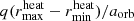 to see if we can find a calibration for the extent of the heating zone. For the three 1D models we computed, we could not see a better calibration with these quantities. Therefore, we kept using the heating parameter Ch as a free parameter in our model.
From the simulations discussed in Sect. 3.2, it is necessary to have two free parameters in our 1D CE model. If we restrict our model to only one free parameter, we cannot reproduce the results of the 3D CE simulations of Sand et al. (2020). Many approximations of our 1D model are captured by the free parameters Cd and Ch. Therefore, the best-fitting values do not directly carry any physical meaning and cannot be immediately used to constrain the physics during CE events.
6. Conclusions
We have presented a 1D approach to simulating the CE evolution within the stellar-evolution code MESA using its hydrodynamic capabilities. The CE is modeled by the envelope of a giant star, in which a point-mass companion is placed on a circular orbit. The viscous forces hinder the motion of the companion because of the dynamical drag by the CE. These extra forces are included in the equations of motion of the companion via a parametric drag-force prescription, allowing us to integrate the orbital evolution of the binary star. The energy lost because of the drag force is added as heat to the envelope. We trace the layers expanding faster than the escape velocity and remove them from the simulated domain. To fit our results to the 3D CE simulations, we include two free parameters, which we use as optimization parameters for the fits.
We simulated the CE phase of a 0.97 M⊙ AGB star and a point-mass companion with mass ratios q = 0.25, 0.50, and 0.75. When comparing and fitting these simulations to the 3D CE simulations of Sand et al. (2020), we come to the following conclusions:
-
It is possible to reproduce the spiral-in curve and the mass fraction of the ejected envelope when using both free parameters for q = 0.25 and 0.50. With one parameter alone, this is not possible. Therefore, 1D CE models similar to ours probably require at least two free parameters to reproduce 3D CE computations. We find that the spiral-in timescale is mostly determined by Cd, while the mass fraction of the ejected envelope is determined by both Cd and Ch.
-
We are unable to find satisfactory fits with the 1D CE model for q = 0.75. This might be an extreme case where the assumptions and approximations of our 1D CE model are no longer valid and do not result in a physical solution.
-
For all mass ratios, we find the post-plunge-in separation in the best-fitting 1D simulation to be smaller than those of the 3D simulation.
-
Regardless of Cd and Ch, the post-plunge-in separation is almost always similar and only depends on the mass ratio. This suggests a deeper physical mechanism that determines the post-plunge-in separation.
-
The recombination energy released from hydrogen and helium likely plays an important role in accelerating and ejecting the envelope.
In a future study, we plan to simulate CE events with different initial configurations (i.e., different masses and evolutionary stages of the giant star) and compare them to 3D CE simulations to investigate whether a global calibration of the two free parameters based on the mass and evolutionary stage of the giant star as well as the mass ratio is possible. If we can find such a calibration, this CE model can be used to predict the outcome of CE events, that is, the post-plunge-in orbital separations and the ejecta mass if the envelope is ejected successfully.
We started the relaxation run with an initial timestep of 10−7 yr and set the maximum timestep during the relaxation run to 10−3 yr.
We only used the radial velocity, vr, in the criterion for envelope ejection, i.e., we neglected the kinetic energy in the rotation of the envelope. We find that excluding the kinetic energy in rotation changes the fraction of the ejected envelope mass in the 3D simulations of Sand et al. (2020) by less than 2% after the end of the dynamical plunge-in phase.
The value of M1, core is taken from Sand et al. (2020) to ensure a meaningful comparison.
We did not simulate the initial phase where the binary star loses co-rotation, but rather started the simulation at the beginning of the plunge-in phase. This was done because the stars have already lost co-rotation according to our setup.
At an optical depth of τ = 10, only e−10 ≈ 0.005% of the photons are expected to escape without any scattering event, compared to ≈ 37% at the photosphere around τ ∼ 1. Initially, Rτ = 1 and Rτ = 10 are spatially separated by ≲10 R⊙, which increases to ≳1000 R⊙ around t = 1500 d. This illustrates the significant difference between τ = 1 and τ = 10. It is worth noting that in 3D simulations, this transition region is difficult to resolve.
The envelope material that is removed during the simulation has fully recombined before reaching velocities higher than the escape velocity (Fig. 4). Thus, the envelope ejection does not remove any potential recombination energy from the system.
The definition of the core mass, M1, core, is arbitrary and can have a huge effect on the value of the binding energy (Tauris & Dewi 2001). For consistency, we used the definition of M1, core = 0.545 M⊙ from Sand et al. (2020) throughout this paper. When using M1, core = 0.540 M⊙, the helium core mass defined by a hydrogen mass fraction less than 0.1, the binding energy of the envelope increases to −5.67 × 1046 erg. Hence, the fractions ΔE/|Ebind, ini| in Fig. 7 should not be used for absolute comparisons.
Acknowledgments
We thank the anonymous referee for their feedback, which helped to improve the quality of the paper. We thank C. Sand for providing the data for the simulations described in Sand et al. (2020). V.A.B., F.R.N.S., Ph.P., and F.K.R. acknowledge support from the Klaus Tschira Foundation. This work has received funding from the European Research Council (ERC) under the European Union’s Horizon 2020 research and innovation programme (Grant agreement No. 945806). This work is supported by the Deutsche Forschungsgemeinschaft (DFG, German Research Foundation) under Germany’s Excellence Strategy EXC 2181/1-390900948 (the Heidelberg STRUCTURES Excellence Cluster). V.A.B. acknowledges support from the International Max Planck Research School for Astronomy and Cosmic Physics at the University of Heidelberg (IMPRS-HD).
References
- Belczynski, K., Kalogera, V., & Bulik, T. 2002, ApJ, 572, 407 [NASA ADS] [CrossRef] [Google Scholar]
- Blöcker, T. 1995, A&A, 299, 755 [Google Scholar]
- Bondi, H., & Hoyle, F. 1944, MNRAS, 104, 273 [Google Scholar]
- Cash, J. R., & Karp, A. H. 1990, ACM Trans. Math. Softw., 16, 201 [CrossRef] [Google Scholar]
- Chamandy, L., Frank, A., Blackman, E. G., et al. 2018, MNRAS, 480, 1898 [NASA ADS] [CrossRef] [Google Scholar]
- Clayton, M., Podsiadlowski, P., Ivanova, N., & Justham, S. 2017, MNRAS, 470, 1788 [NASA ADS] [CrossRef] [Google Scholar]
- Courant, R., Friedrichs, K., & Lewy, H. 1928, Math. Ann., 100, 32 [Google Scholar]
- De Marco, O., & Izzard, R. G. 2017, PASA, 34, e001 [Google Scholar]
- Detmers, R. G., Langer, N., Podsiadlowski, P., & Izzard, R. G. 2008, A&A, 484, 831 [NASA ADS] [CrossRef] [EDP Sciences] [Google Scholar]
- Eldridge, J. J., & Stanway, E. R. 2016, MNRAS, 462, 3302 [Google Scholar]
- Fragos, T., Andrews, J. J., Ramirez-Ruiz, E., et al. 2019, ApJ, 883, L45 [Google Scholar]
- Fryer, C. L., & Woosley, S. E. 1998, ApJ, 502, L9 [NASA ADS] [CrossRef] [Google Scholar]
- Glanz, H., & Perets, H. B. 2018, MNRAS, 478, L12 [NASA ADS] [CrossRef] [Google Scholar]
- Grott, M., Chernigovski, S., & Glatzel, W. 2005, MNRAS, 360, 1532 [NASA ADS] [CrossRef] [Google Scholar]
- Han, Z., Podsiadlowski, P., & Eggleton, P. P. 1995, MNRAS, 272, 800 [NASA ADS] [Google Scholar]
- Heber, U. 2009, ARA&A, 47, 211 [Google Scholar]
- Hirai, R., & Mandel, I. 2022, ApJ, 937, L42 [NASA ADS] [CrossRef] [Google Scholar]
- Hoyle, F., & Lyttleton, R. A. 1939, Proc. Cambridge Philos. Soc., 35, 405 [Google Scholar]
- Hoyle, F., & Lyttleton, R. A. 1941, MNRAS, 101, 227 [NASA ADS] [Google Scholar]
- Iaconi, R., & De Marco, O. 2019, MNRAS, 490, 2550 [Google Scholar]
- Iaconi, R., Reichardt, T., Staff, J., et al. 2017, MNRAS, 464, 4028 [NASA ADS] [CrossRef] [Google Scholar]
- Iaconi, R., Maeda, K., Nozawa, T., De Marco, O., & Reichardt, T. 2020, MNRAS, 497, 3166 [NASA ADS] [CrossRef] [Google Scholar]
- Iben, I., Jr., & Tutukov, A. V. 1984, ApJS, 54, 335 [NASA ADS] [CrossRef] [Google Scholar]
- Ivanova, N., & Nandez, J. L. A. 2016, MNRAS, 462, 362 [NASA ADS] [CrossRef] [Google Scholar]
- Ivanova, N., Justham, S., Chen, X., et al. 2013, A&A Rev, 21, 59 [NASA ADS] [CrossRef] [Google Scholar]
- Ivanova, N., Justham, S., & Podsiadlowski, P. 2015, MNRAS, 447, 2181 [Google Scholar]
- Izzard, R. G., Ramirez-Ruiz, E., & Tout, C. A. 2004, MNRAS, 348, 1215 [NASA ADS] [CrossRef] [Google Scholar]
- John, J. A., & Draper, N. R. 1980, J. Roy. Stat. Soc.: Ser. C (Appl. Stat.), 29, 190 [Google Scholar]
- Kim, W.-T. 2010, ApJ, 725, 1069 [NASA ADS] [CrossRef] [Google Scholar]
- Kim, H., & Kim, W.-T. 2007, ApJ, 665, 432 [NASA ADS] [CrossRef] [Google Scholar]
- Kramida, A., Ralchenko, Y., Reader, J., & NIST ASD Team 2021, NIST Atomic Spectra Database (ver. 5.9), [Online, 2022, August 10] (Gaithersburg, MD: National Institute of Standards and Technology) [Google Scholar]
- Kruckow, M. U., Tauris, T. M., Langer, N., Kramer, M., & Izzard, R. G. 2018, MNRAS, 481, 1908 [CrossRef] [Google Scholar]
- Lau, M. Y. M., Hirai, R., González-Bolívar, M., et al. 2022a, MNRAS, 512, 5462 [NASA ADS] [CrossRef] [Google Scholar]
- Lau, M. Y. M., Hirai, R., Price, D. J., & Mandel, I. 2022b, MNRAS, 516, 4669 [NASA ADS] [CrossRef] [Google Scholar]
- Livio, M., & Soker, N. 1988, ApJ, 329, 764 [Google Scholar]
- Mandel, I., & Broekgaarden, F. S. 2022, Liv. Rev. Relat., 25, 1 [Google Scholar]
- Marchant, P., Pappas, K. M. W., Gallegos-Garcia, M., et al. 2021, A&A, 650, A107 [NASA ADS] [CrossRef] [EDP Sciences] [Google Scholar]
- Meyer, F., & Meyer-Hofmeister, E. 1979, A&A, 78, 167 [NASA ADS] [Google Scholar]
- Moreno, M. M., Schneider, F. R. N., Röpke, F. K., et al. 2022, A&A, 667, A72 [NASA ADS] [CrossRef] [EDP Sciences] [Google Scholar]
- Nandez, J. L. A., Ivanova, N., & Lombardi, J. C., Jr 2014, ApJ, 786, 39 [NASA ADS] [CrossRef] [Google Scholar]
- O’Connor, C. E., Bildsten, L., Cantiello, M., & Lai, D. 2023, ApJ, 950, 128 [CrossRef] [Google Scholar]
- Ohlmann, S. T., Röpke, F. K., Pakmor, R., & Springel, V. 2016a, ApJ, 816, L9 [Google Scholar]
- Ohlmann, S. T., Röpke, F. K., Pakmor, R., Springel, V., & Müller, E. 2016b, MNRAS, 462, L121 [NASA ADS] [CrossRef] [Google Scholar]
- Ondratschek, P. A., Röpke, F. K., Schneider, F. R. N., et al. 2022, A&A, 660, L8 [NASA ADS] [CrossRef] [EDP Sciences] [Google Scholar]
- Ostriker, E. C. 1999, ApJ, 513, 252 [Google Scholar]
- Paczyński, B. 1976, in Structure and Evolution of Close Binary Systems, eds. P. Eggleton, S. Mitton, & J. Whelan, 73, 75 [NASA ADS] [CrossRef] [Google Scholar]
- Passy, J.-C., De Marco, O., Fryer, C. L., et al. 2012, ApJ, 744, 52 [NASA ADS] [CrossRef] [Google Scholar]
- Paxton, B., Bildsten, L., Dotter, A., et al. 2011, ApJS, 192, 3 [Google Scholar]
- Paxton, B., Cantiello, M., Arras, P., et al. 2013, ApJS, 208, 4 [Google Scholar]
- Paxton, B., Marchant, P., Schwab, J., et al. 2015, ApJS, 220, 15 [Google Scholar]
- Paxton, B., Schwab, J., Bauer, E. B., et al. 2018, ApJS, 234, 34 [NASA ADS] [CrossRef] [Google Scholar]
- Paxton, B., Smolec, R., Schwab, J., et al. 2019, ApJS, 243, 10 [Google Scholar]
- Podsiadlowski, P. 2001, in Evolution of Binary and Multiple Star Systems, eds. P. Podsiadlowski, S. Rappaport, A. R. King, F. D’Antona, & L. Burderi, ASP Conf. Ser., 229, 239 [NASA ADS] [Google Scholar]
- Podsiadlowski, P., Joss, P. C., & Hsu, J. J. L. 1992, ApJ, 391, 246 [Google Scholar]
- Prohaska, T., Irrgeher, J., Benefield, J., et al. 2022, Pure Appl. Chem., 94, 573 [CrossRef] [Google Scholar]
- Prust, L. J., & Chang, P. 2019, MNRAS, 486, 5809 [NASA ADS] [CrossRef] [Google Scholar]
- Reichardt, T. A., De Marco, O., Iaconi, R., Tout, C. A., & Price, D. J. 2019, MNRAS, 484, 631 [NASA ADS] [CrossRef] [Google Scholar]
- Reichardt, T. A., De Marco, O., Iaconi, R., Chamandy, L., & Price, D. J. 2020, MNRAS, 494, 5333 [NASA ADS] [CrossRef] [Google Scholar]
- Reimers, D. 1975, Mémoires of the Société Royale des Sciences de Lièege, 8, 369 [Google Scholar]
- Ricker, P. M., & Taam, R. E. 2008, ApJ, 672, L41 [NASA ADS] [CrossRef] [Google Scholar]
- Ricker, P. M., & Taam, R. E. 2012, ApJ, 746, 74 [Google Scholar]
- Röpke, F. K., & De Marco, O. 2023, Liv. Rev. Comput. Astrophys., 9, 2 [CrossRef] [Google Scholar]
- Sand, C., Ohlmann, S. T., Schneider, F. R. N., Pakmor, R., & Röpke, F. K. 2020, A&A, 644, A60 [NASA ADS] [CrossRef] [EDP Sciences] [Google Scholar]
- Shiber, S., Iaconi, R., De Marco, O., & Soker, N. 2019, MNRAS, 488, 5615 [NASA ADS] [CrossRef] [Google Scholar]
- Spera, M., Mapelli, M., Giacobbo, N., et al. 2019, MNRAS, 485, 889 [Google Scholar]
- Stevenson, S., Vigna-Gómez, A., Mandel, I., et al. 2017, Nat. Commun., 8, 14906 [Google Scholar]
- Taam, R. E., Bodenheimer, P., & Ostriker, J. P. 1978, ApJ, 222, 269 [NASA ADS] [CrossRef] [Google Scholar]
- Tauris, T. M., & Dewi, J. D. M. 2001, A&A, 369, 170 [NASA ADS] [CrossRef] [EDP Sciences] [Google Scholar]
- Tauris, T. M., & van den Heuvel, E. P. J. 2006, Compact Stellar X-ray Sources (Cambridge, UK: Cambridge University Press), 39, 623 [NASA ADS] [CrossRef] [Google Scholar]
- Toro, E. F., Spruce, M., & Speares, W. 1994, Shock Waves, 4, 25 [Google Scholar]
- Trani, A. A., Rieder, S., Tanikawa, A., et al. 2022, Phys. Rev. D, 106, 043014 [NASA ADS] [CrossRef] [Google Scholar]
- Tutukov, A. V., & Yungelson, L. R. 1993, MNRAS, 260, 675 [Google Scholar]
- Vigna-Gómez, A., Neijssel, C. J., Stevenson, S., et al. 2018, MNRAS, 481, 4009 [Google Scholar]
- Voss, R., & Tauris, T. M. 2003, MNRAS, 342, 1169 [Google Scholar]
- Warner, B. 1995, Cataclysmic Variable Stars (Cambridge Atmospheric Space Science Series), 28 [CrossRef] [Google Scholar]
- Webbink, R. F. 1984, ApJ, 277, 355 [NASA ADS] [CrossRef] [Google Scholar]
- Whelan, J., & Iben, I., Jr. 1973, ApJ, 186, 1007 [Google Scholar]
- Yarza, R., Everson, R. W., & Ramirez-Ruiz, E. 2022, arXiv e-prints [arXiv:2210.00010] [Google Scholar]
Appendix A: Resolution study
To prove the robustness of the results we obtained with our 1D CE method described in Sect. 2, we performed a small resolution study. We reran the simulations for q = 0.25, presented in Sect. 3. For one simulation, we increased the time resolution by a factor of 2, and for a second simulation we decreased the spatial resolution by a factor of 1.6. The results of these simulations are shown in Fig. A.1.
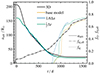 |
Fig. A.1. Similar to Fig. 2, but also showing the simulation at a lower spatial resolution and at a higher time resolution. |
The spiral in the behavior of the companion is mostly unchanged when compared to the original simulation. There are, however, some differences in the envelope ejection between the different simulations. The exact timing of the main envelope-ejection event varies by about 100 d. In addition, the shape of the ejection curve also depends on the resolution. Once a more continuous ejection is established after the main ejection events at t = 900 − 1000 d, the values of fej only vary by 5%, which is within our expected tolerances.
The reason for the differences in the envelope ejection originates mostly from differences in the surface properties between the simulations. As described in Sect. 2.3, we performed a relaxation run before the CE simulations where we switched the outer boundary condition and turned on the hydro mode. These changes cause small amplitude oscillations close to the surface of the CE (see also Fig. 4a). The oscillations are stochastic and therefore so are some of the surface properties, for example the surface velocity. This means that the exact timing of when the surface velocity exceeds the escape velocity has a minor dependence on the initial oscillations. This causes the difference in the starting time of the ejection. The total ejected mass toward the end of the simulations, the quantity in which we are mostly interested varies within our tolerances.
Based on this resolution study, we conclude that the final values for the orbital separation do not depend on the resolution. The total ejecta mass has a minor dependence on the resolution but varies within our tolerances of a few percent.
All Tables
All Figures
|
Fig. 1. Initial density profile ρini, 1D of the AGB star in comparison to the initial density profile ρini, 3D of the AGB star in Sand et al. (2020), as well as the 1D and 3D density profiles after the relaxation run, ρrelax, 1D and ρrelax, 3D. Relative deviations between the density profiles are shown along the secondary ordinate. |
| In the text | |
|
Fig. 2. Best-fitting 1D CE simulation for q = 0.25 when comparing to the 3D CE simulation of Sand et al. (2020). Full lines show the orbital separation, and the dotted and dash-dotted lines show the mass fraction of ejected envelope fej and fej, all, respectively. The results of the 3D simulations are shown in orange, and the results from this work are shown in blue. The vertical dashed gray line indicates the end of the dynamical plunge-in phase as determined by Eq. (22). The 3D simulation results are all shifted by Δtmin = −58 d to compensate for the difference in the initial separation. The gray shaded region shows t < 0 d, for which we cannot compare the 1D simulation to the 3D simulation. |
| In the text | |
|
Fig. 3. Effects of Cd and Ch on the spiral-in curves, aorb, and the envelope-ejection fraction, fej. In panel a the heating parameter is held constant at Ch = 4.00 and the drag-force parameter, Cd, is varied. In panel b the drag-force parameter is held constant at Cd = 0.23 and the heating parameter, Ch, is varied. The thick black lines in both panels show the results from the 3D hydrodynamic CE simulation of Sand et al. (2020), which are shifted by Δtmin = −58 d, the time shift determined using the best-fitting 1D simulation with Cd = 0.23 and Ch = 4.00. |
| In the text | |
|
Fig. 4. Kippenhahn diagrams of the simulation with q = 0.25, Cd = 0.23, and Ch = 4.0. In panel a, the radial velocity is shown in terms of the local escape velocity; layers colored in red have a radial velocity higher than the local escape velocity. Panels b, c, and d show the ionization fractions of H II, HeII, and He III, respectively. The heating kernel as described in Eq. (15) is shown in panel e, and the specific heating rate in panel f. The red line indicates the orbital separation between the companion and the core of the giant star. The dotted gray region is heated during the CE simulation. The dashed cyan line shows Rτ = 10, which traces the hydrogen-recombination radius. The dashed gray lines represent envelope-mass fractions of 0.95, 0.9, 0.8, 0.6, 0.4, 0.2, 0.1, 0.06, 0.04, and 0.03 from the surface toward the center, and visualize the expansion of the envelope. The white patches in panel a show layers that have an inward (negative) radial velocity. |
| In the text | |
|
Fig. 5. Kippenhahn diagrams (similar to Fig. 4) of the simulation with q = 0.25, Cd = 0.23, and Ch = 4.0, showing the Mach number (ℳ= vr/cs) in panel a, velocity divergence (dv/dr) in panel b, specific entropy (s) in panel c, and opacity (κ) in panel d. The white hatched zones in panel c indicate convective mixing. For a better visualization of the velocity divergence, the log modulus transformation, logmod(x) = sgn(x)log10(|x|+1), is used (John & Draper 1980). The arrows in panel b roughly indicate the recombination zones of H I, He I, and He II (see also Figs. 4b–d). |
| In the text | |
|
Fig. 6. Fraction of released recombination energy (frec) and contributions of hydrogen (H II), singly ionized helium (He II), and doubly ionized helium (He III) for the simulation with q = 0.25, Cd = 0.23, and Ch = 4.0. The total fraction of released recombination energy is shown in black. The horizontal dashed colored lines show the initially available recombination energy in each species. The vertical dashed gray line indicates the end of the dynamical plunge-in phase as determined by Eq. (22). |
| In the text | |
|
Fig. 7. Major energy sources (dashed lines) and sinks (solid lines) during the CE simulation with q = 0.25, Cd = 0.23, and Ch = 4.0. Shown are the total injected energy, ΔEheat, the change in internal energy, ΔEint, the total released recombination energy, ΔErec (the recombination energy is part of the internal energy and is only shown separately to highlight the contribution from recombination), the change in orbital energy, ΔEorb, according to Eq. (34), the extra term ΔEm defined by Yarza et al. (2022), the change in the gravitational energy, ΔEgrav, and the energy that is carried away by radiation, ΔErad. The vertical dashed gray line indicates the end of the dynamical plunge-in phase as determined by Eq. (22). The energies are shown in units of the initial binding energy of the envelope with Ebind, ini = −4.03 × 1045 erg, calculated via Eq. (32). The lines showing contributions from ΔEorb and ΔEm are dash-dotted as they show source terms for the heating ΔEheat but are not direct energy sources in the MESA simulation. |
| In the text | |
|
Fig. 8. Time evolution of the drag force and its components for q = 0.25, Cd = 0.23, and Ch = 4.0. The visualization of these quantities represents how each of them enters the drag force according to Eq. (5). The drag force is in the nonlinear regime, i.e., ℳ > 1.01 and ηℬ > 0.1, during the whole simulation. The ratio between the drag force and the gravitational force, Fg, is also shown. The vertical dashed gray line indicates the end of the dynamical plunge-in phase as determined by Eq. (22). |
| In the text | |
|
Fig. 9. Similar to Fig. 2, but showing the best-fitting 1D simulation compared to the 3D simulation of Sand et al. (2020) for mass ratios q = 0.5 (panel a) and q = 0.75 (panel b). |
| In the text | |
|
Fig. A.1. Similar to Fig. 2, but also showing the simulation at a lower spatial resolution and at a higher time resolution. |
| In the text | |
Current usage metrics show cumulative count of Article Views (full-text article views including HTML views, PDF and ePub downloads, according to the available data) and Abstracts Views on Vision4Press platform.
Data correspond to usage on the plateform after 2015. The current usage metrics is available 48-96 hours after online publication and is updated daily on week days.
Initial download of the metrics may take a while.