| Issue |
A&A
Volume 644, December 2020
|
|
|---|---|---|
| Article Number | A84 | |
| Number of page(s) | 35 | |
| Section | Interstellar and circumstellar matter | |
| DOI | https://doi.org/10.1051/0004-6361/202038966 | |
| Published online | 02 December 2020 | |
The GUAPOS project: G31.41+0.31 Unbiased ALMA sPectral Observational Survey
I. Isomers of C2H4O2★
1
Dipartimento di Fisica e Astronomia, Università degli Studi di Firenze,
Via Sansone 1,
50019
Sesto Fiorentino, Italy
e-mail: chiara.mininni.astro@gmail.com; chiara.mininni@unifi.it
2
INAF Osservatorio Astrofisico di Arcetri,
Largo E. Fermi 5,
50125
Firenze, Italy
3
Centro de Astrobiología (CSIC, INTA),
Ctra. de Ajalvir, km. 4,
Torrejón de Ardoz,
28850
Madrid, Spain
4
I. Physikalisches Institut, Universität zu Köln,
Zülpicher Str. 77,
50937
Köln, Germany
5
Leiden Observatory, Leiden University, PO Box 9513,
NL-2300 RA
Leiden, The Netherlands
6
European Southern Observatory (ESO),
Karl-Schwarzschild-Str. 2,
85748
Garching, Germany
7
Department of Physics and Astronomy, UCL,
Gower Place,
London
WC1E 6BT, UK
Received:
18
July
2020
Accepted:
22
September
2020
Context. One of the goals of astrochemistry is to understand the degree of chemical complexity that can be reached in star-forming regions, along with the identification of precursors of the building blocks of life in the interstellar medium. To answer such questions, unbiased spectral surveys with large bandwidth and high spectral resolution are needed, in particular, to resolve line blending in chemically rich sources and identify each molecule (especially for complex organic molecules). These kinds of observations have already been successfully carried out, primarily towards the Galactic Center, a region that shows peculiar environmental conditions.
Aims. We present an unbiased spectral survey of one of the most chemically rich hot molecular cores located outside the Galactic Center, in the high-mass star-forming region G31.41+0.31. The aim of this 3mm spectral survey is to identify and characterize the physical parameters of the gas emission in different molecular species, focusing on complex organic molecules. In this first paper, we present the survey and discuss the detection and relative abundances of the three isomers of C2H4O2: methyl formate, glycolaldehyde, and acetic acid.
Methods. Observations were carried out with the ALMA interferometer, covering all of band 3 from 84 to 116 GHz (~32 GHz bandwidth) with an angular resolution of 1.2′′ × 1.2′′ (~ 4400 au × 4400 au) and a spectral resolution of ~0.488 MHz (~1.3−1.7 km s−1). The transitions of the three molecules have been analyzed with the software XCLASS to determine the physical parameters of the emitted gas.
Results. All three isomers were detected with abundances of (2 ± 0.6) × 10−7, (4.3−8) × 10−8, and (5.0 ± 1.4) × 10−9 for methyl formate, acetic acid, and glycolaldehyde, respectively. Methyl formate and acetic acid abundances are the highest detected up to now, if compared to sources in the literature. The size of the emission varies among the three isomers with acetic acid showing the most compact emission while methyl formate exhibits the most extended emission. Different chemical pathways, involving both grain-surface chemistry and cold or hot gas-phase reactions, have been proposed for the formation of these molecules, but the small number of detections, especially of acetic acid and glycolaldehyde, have made it very difficult to confirm or discard the predictions of the models. The comparison with chemical models in literature suggests the necessity of grain-surface routes for the formation of methyl formate in G31, while for glycolaldehyde both scenarios could be feasible. The proposed grain-surface reaction for acetic acid is not capable of reproducing the observed abundance in this work, while the gas-phase scenario should be further tested, given the large uncertainties involved.
Key words: astrochemistry / ISM: molecules / stars: formation / ISM: individual objects: G31.41+0.31
Tables C.1–C.3 are only available at the CDS via anonymous ftp to cdsarc.u-strasbg.fr (130.79.128.5) or via http://cdsarc.u-strasbg.fr/viz-bin/cat/J/A+A/644/A84
© ESO 2020
1 Introduction
Hot molecular cores (HMCs), the birthplaces of massive stars, are the sources that show the highest level of chemical complexity in the Galaxy (Herbst & van Dishoeck 2009). Their spectra include emission from a large variety of molecules, starting from the simplestdiatomic species up through complex organic molecules (COMs), which are molecules containing carbon withsix or more atoms. In recent years, our view and comprehension of the chemistry of the interstellar medium (ISM) has improved substantially and species with up to 13 atoms have been unambiguously detected (c-C6 H5CN, McGuire et al. 2018). The advent of more sensitive instruments with high spectral and spatial resolution, such as ALMA (Atacama Large Millimeter Array), has allowed the detection of emission from faint molecular species, particularly heavy COMs sincethese typically emit a large number of transitions that could be faint or blended with those of other molecules.
This chemically rich environment and the presence of several COMs is thought to be the result of the evaporation of the products of grain-surface reactions thanks to the presence of an already formed proto-stellar object(s), which starts to heat up the surrounding medium, and of the subsequent hot gas-phase chemistry. The detection of COMs in cold environments as well (Öberg et al. 2010; Bacmann et al. 2012; Vastel et al. 2014; Jiménez-Serra et al. 2016) has opened up new scenarios and other possible chemical routes in cold gas-phase have been proposed to explain these observations (i.e., Vasyunin & Herbst 2013; Balucani et al. 2015; Vasyunin et al. 2017). Thus, it is possible that in HMCs, some of the observed COMs emission is also inherited from the cold chemistry at early stages of the star-formation process. Hence, these new routes need to be considered in chemical models.
To investigate the maximum degree of chemical complexity in star-forming regions, spectral surveys have been carried out towards a few sources, of both high-mass and low-mass cores (Kalenskii & Johansson 2010; Belloche et al. 2016; Jørgensen et al. 2016). One of the most studied sources is SgrB2 (Belloche et al. 2013, 2016, 2019; Sánchez-Monge et al. 2017), although the environmental conditions of this source, cataloged as a mini-starbust region, cannot be considered as typical of HMCs because its peculiar environment is likely to have had an impact on the chemistry.
With this in mind, we decided to perform a spectral survey covering the entire ALMA band 3 towards one of the most chemically rich HMCs outside the Galactic Center (GC), G31.41+0.31 (hereafter G31), where glycolaldehyde (CH2 OHCHO, GA) has been detected for the first time outside the GC (Beltrán et al. 2009).
The target of the G31.41+0.31 Unbiased ALMA sPectral Observational Survey (GUAPOS) is a well-known and studied HMC located at a distance of 3.75 kpc (Immer et al. 2019) with a luminosity of 4.4 × 10⁴ L⊙ (from Osorio et al. 2009)and a mass M ~ 70 M⊙ (Cesaroni 2019), after rescaling to the new distance estimate (the previous distance estimate was of 7.9 kpc). The source was first detected in NH3(4, 4) (Cesaroni et al. 1994a), whose emission was co-spatial to the distribution of water masers (Hofner & Churchwell 1993), and separated by ~ 5′′ from an already known ultra compact (UC) HII region. Cesaroni et al. (1994b) discovered a velocity gradient of ~ 400 km s−1 pc−1 across the core in the emission of methyl cyanide (CH3CN) at 3 mm, along the SW-NE direction. The nature of this velocity gradient was further investigated in more recent studies and is most likely associated with a rotating toroid with a spin up toward the center (Beltrán et al. 2004, 2005, 2018; Cesaroni et al. 2010, 2011, 2017). Although another interpretation in terms of expansion was proposed (Gibb et al. 2004; Araya et al. 2008), this is inconsistent with recent polarization observations (Beltrán et al. 2019). These studies revealed also the presence of several outflows, traced by CO and SiO emission (Cesaroni et al. 2011; Beltrán et al. 2018), of infalling material (firstly found by Girart et al. 2009; see also Mayen-Gijon et al. 2014 and Beltrán et al. 2018) and of two free–free sources at 0.7 and 1.3 cm separated by 0′′.19 embedded in the core (Cesaroni et al. 2010).
G31 has also been studied in polarized emission at mm wavelengths by Girart et al. (2009) and, recently, by Beltrán et al. (2019). The reconstructed shape of the magnetic field follows an hourglass morphology, with the best model of Beltrán et al. (2019) suggesting a predominant poloidal field, oriented perpendicular to the SW-NE velocity gradient previously detected in G31, lending strong support to the rotating toroid scenario, as already mentioned.
G31 has also been studied from a chemical point of view, revealing one of the most striking features of this HMC: its chemical richness. As previously mentioned, the first detection of glycolaldehyde outside the GC was obtained towards G31 (Beltrán et al. 2009), and confirmed by Calcutt et al. (2014) and Rivilla et al. (2017). Other heavy COMs such as ethyl cyanide C2 H5 CN, dimethyl ether CH3OCH3, ethanol C2H5OH, and ethylene glycol  (nine, nine, nine, and ten atoms respectively) were also detected here (Beltrán et al. 2005; Fontani et al. 2007; Isokoski et al. 2013; Rivilla et al. 2017; Coletta et al. 2020). The chemical richness of this HMC has been quantified by Cesaroni et al. (2017), who reported that the fraction of channels with line emission was 0.74 (the largest in the sample of high-mass young stellar objects studied by these authors) in the 217–237 GHz range. G31 is, thus, one of the best candidates for investigating the degree of chemical complexity that can be reached in typical high-mass star-forming regions.
Among COMs, a special class of molecules is made up of isomers, which are molecules with the same chemical composition, but with a different molecular structure. These molecules can be used to explore which chemical formation pathway is more efficient, leading to a predominance of one isomer with respect to the other(s) and helping to constrain the chain of chemical reactions involved in their formation. Among isomers, those of C2 H4 O2 (see Fig. 1), namely glycolaldehyde (CH2OHCHO, hereafter GA), methyl formate (CH3OCHO, hereafter MF), and acetic acid (CH3COOH, hereafter AA), are especially interesting because of their relevance for the formation of prebiotic molecules. In fact, GA is the simplest sugar-related molecule and can react with propenal to form ribose, an essential constituent of RNA. The three molecules were all firstly detected towards SgrB2 (Brown et al. 1975; Mehringer et al. 1997; Hollis et al. 2000). MF has been detected in a large number of objects including high-mass star-forming regions (Beuther et al. 2007; Fontani et al. 2007; Favre et al. 2014; Sakai et al. 2015; Belloche et al. 2016), low-mass star-forming regions (Cazaux et al. 2003; Bottinelli et al. 2007; Jørgensen et al. 2012; Jacobsen et al. 2019), prestellar cores (Bacmann et al. 2012; Jiménez-Serra et al. 2016), cold envelopes around protostars (Öberg et al. 2010; Cernicharo et al. 2012), and outflow and shock regions (Arce et al. 2008; Csengeri et al. 2019). On the other hand, the number of detections of GA and AA is limited compared to that of methyl formate, despite the presence of dedicated surveys (e.g., Remijan et al. 2003). In the literature, there are few star-formingregions in which all three isomers have been detected: SgrB2(N)-LMH (Hollis et al. 2001; Belloche et al. 2013; Xue et al. 2019), the two HMCs NGC 6334I MM1 & MM2 (El-Abd et al. 2019), and the low-mass sources IRAS16293-2422B and IRAS16293-2422A (Jørgensen et al. 2012, 2016; Manigand et al. 2020). To better constrain and compare thepredictions of the chemical models with observations, more sources with all three isomers detected are needed.
GA was firstly detected outside the GC towards G31 (Beltrán et al. 2009), where Isokoski et al. (2013), Calcutt et al. (2014), and Rivilla et al. (2017) detected MF.
The aim of this work is to present the GUAPOS project1 and to focus on the simulaneous analysis of the 3 C2 H4O2 isomers: GA, MF, and AA. In Sect. 2, we describe the observations and the data reduction process for obtaining the final spectra. In Sect. 3, we analyze the continuum emission and describe the methodology for the spectral analysis of the three isomers of C2H4O2. In Sect. 4, we show the result for MF, AA, and GA. In Sect. 5, we discuss the abundances and the column density ratios among the three isomers and compare them with previous values in the literature and with the predictions of different chemical models to better understand how this COMs are formed in the ISM of star-forming regions. Finally in Sect. 6, we summarize our conclusions.
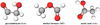 |
Fig. 1 Chemical structures of the three isomers of C2H4O2. |
2 Observations and data reduction
2.1 Observations
The observations were carried out with ALMA during Cycle 5, between 18 January and 7 September 2018 (project 2017.1.00501.S, P.I.: M. T. Beltrán), using 43 antennas. The coordinates of phase center, together with other properties of G31, are given in Table 1. More details about the spectral setup, the baselines, and the flux and phase calibrators are given in Table 2. The survey covers the complete spectral range of ALMA band 3, between 84.05 and 115.91 GHz (~ 32 GHz bandwidth), with a spectral resolution of ~0.488 MHz (~ 1.3−1.7 km s−1). We used nine correlator configurations (spec) and for each of them, four contiguous basebands of ~ 937 MHz were observed simultaneously. In order to create a single spectrum starting from the 36 spectra of the respective basebands, an overlap in frequency ranging from ~7.3 to ~ 29 MHz was chosen for each pair of adjacent basebands. The original angular resolution requested in the proposal (1′′) was not achieved for two out of nine specs (spec 3 and 4) during the observations between January and March 2018. Although we were granted additional observing time for these two specs, the new observations did not reach the angular resolution required either, achieving only ~ 1.′′2. We decided to degrade the angular resolution of all the specs to the lowest one (~ 1.′′2) to have the same spatial resolution for all of them. For all the specs, the source used as flux and bandpass calibrator isJ1751+0939, while J1851+0035 is the phase calibrator. The uncertainties in the flux calibration are ~ 5% (from Quality Assesment 2 reports), which is in good agreement with flux uncertainties of other ALMA band 3 calibrators reported in Bonato et al. (2018).
The data were calibrated and imaged with Common Astronomy Software Applications2 (CASA package, McMullin et al. 2007). The maps were created using a robust parameter of Briggs (1995) set equal to 0 and a restoring synthesized beam of 1′′.2 × 1.′′2. The root mean square (rms) of the maps varies between 0.5 and 1.9 mJy beam−1.
Coordinates used for the observations and main parameters of the source G31.
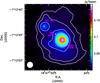 |
Fig. 2 Continuum map of the HMC G31.41+0.31 and the nearby UC HII region. Contour levels are at 5, 10, 20, 40, 60, 100, and 200 times the value of rms = 0.8 mJy beam−1. The three white triangles indicate the coordinates of the Main Core and NE core by Beltrán et al. (2018), and of the UC HII region by Cesaroni et al. (1998). The beam is shown in white in the lower left corner. |
2.2 Continuum determination
Due to the large number of lines in the spectra, it was not possible to find a sufficient number of channels without line emission that could be used to obtain a map of the continuum emission. To overcome this problem we used STATCONT (Sánchez-Monge et al. 2018), a python-based tool designed to determine the continuum emission level in spectral data, particularly for sources with a very rich spectrum. This tool determines the continuum level by using a statistical approach on the intensity distribution of the spectrum and produces a continuum map. We obtained the continuum map (Fig. 2) from the line+continuum map of the spec5 BB1 (see Table 2, ν : 98 499.749−99 436.626 MHz) in order to have the continuum extracted from a frequency close to the center of the frequency range covered by the GUAPOS observations (~ 84−116 GHz).
Spectral setup of observations.
2.3 Combination of the spectral windows
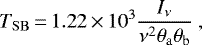
From each baseband, we extracted the mean spectrum inside an area equal to the beam, centered at the position of the continuum peak of the HMC (see coordinates in Sect. 3.1). This area is smaller than the size of the continuum core (see Sect. 3.1 and Fig. 2). In the Rayleigh-Jeans approximation, the relation between the synthesized beam brightness temperature TSB [K] and the flux Iν [mJy beam−1] is:
 (1)
(1)
where ν is the frequency in units GHz and θa and θb are the major and minor axes of the synthesized beam in arcsec. The discrepancy between the TSB and the physical temperature of a thermalized, beam-filling source emitting the same Iν, is of the order of ~ 15% for the channels with only continuum emission, and only of the ~3% for the channels with bright-line emission. Adjacent spectra have been merged to produce a single final spectrum thanks to the overlapping regions between each pair of adjacent basebands. Since jumps up to 3 K are present between partially overlapping adjacent spectra, we adopt the following procedure to create the merged spectrum. We align the spectra from the different basebands using the spectrum at longer λ (spec1 BB1, see Table 2) as reference. In practice, we forced the channels of spec1 BB2 in the overlapping region to match those of spec1 BB1 by subtracting from spec1 BB2 the mean value of the difference between spec1 BB2 and spec1 BB1. We define this mean value as b1. Then the procedure was repeated for all the other pairs (spec1 BB2 and spec1 BB3, spec1BB3 and spec1 BB4,spec1 BB4, and spec2 BB1 etc.) thus obtaining a single spectrum without artificial jumps and the values, bi, of the baselines of the spectra of all the basebands with respect to the reference one. As a last step, we shifted the final spectrum without jumps by a value equal to the mean of bi to obtain a final spectrum without jumps with a baseline equal to the mean value of the baselines of the original spectra. Figure 3 summarizes and graphically illustrates the main steps described above.
We converted the spectra to rest frequency, assuming a velocity of the source of 96.5 km s−1, and rebinned the spectra to a constant value of the bin width equal to 0.48840 MHz using Herschel Interactive Processing Environment3 (HIPE, Ott 2010) since the small differences in the bandwidth of different basebands lead to differences in the channel widths (see Table 2), which span between 0.48837 and 0.48845 MHz (after the conversion to rest frequency). This was done also considering the possibility of analyzing the spectrum with different software since some of the commonly used software to analyze spectra (e.g., CLASS or MADCUBA4) need a unique frequency width to import the data.
We remark that the procedure we used did not, in principle, affect the slope of the baseline in each baseband in any way. Considering the artificial nature of the jumps in adjacent spectra, we expect the slope of the baseline not to be shifted considerablyfrom its true value.
The rms at the level of the baseline, calculated as the rms of the differences between the original baseline in each baseband and the baseline in the final spectrum, is 1.2 K (~ 12% of the continuum level, see Sect. 3.1). This 12% error on the continuum level is included as additional error on theparameters derived from the fit to the spectrum. The rms of the spectra has been derived from the rms of the maps (see Table 2) and vary from 7 to 27 mK, for the different basebands, but we consider a conservative value of 27 mK for the entire final spectrum. The fluctuations in the rms of the maps are the result of different atmospheric conditions in different days of observations and of the presence of bright lines in some of the basebands (therefore, a dynamic range effect). Figure 4 shows the total final spectrum.
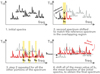 |
Fig. 3 Graphic scheme of the steps followed to obtain the final spectrum. |
3 Analysis
3.1 Continuum
The map of the continuum (see Fig. 2) shows the presence of two compact sources. The brightest source is our target, HMC G31.41+0.31, which peaks at RA 18h 47m 34.321s Dec − 01° 12′ 45.977′′ (J2000). Located at a distance of ~ 4.′′5 in the NE direction, there is a fainter continuum source that peaks at RA 18h 47m 34.56s Dec − 01°12′ 43.35′′ (J2000), which is consistent with the position of the nearby UC HII region observed by Cesaroni et al. (1998) in the continuum at 1.3 cm with the VLA. The NE core, identified by Beltrán et al. (2018) with high resolution observations, is not resolved in our data at 1′′.2, resolution.
We fitted a 2D Gaussian to the continuum emission of the main core using the task imfit of CASA and obtained the source size of the HMC, reported in Table 3. The source is barely resolved, with the deconvolved size of the continuum being 1′′.41 × 1.′′22.
The flux of the continuum inside the area from which we extracted the spectrum is of 0.1 Jy at the mean frequency of 99.0 GHz (see Sect. 2.2). Assuming a dust temperature of 150 K, β = 2.0, a dust opacity coefficient k0 = 0.8 cm2 g−1 at 220 GHz (Ossenkopf & Henning 1994), a mean molecular weight of 2.33, and a gas-to-dust ratio of 100, we have a column density of H2 is N(H2) = 1.0 × 1025 cm−2. This value is consistent within a factor ~4 with the previous estimate by Rivilla et al. (2017).
We have fitted by eye the continuum level of the spectrum assuming a power law,
 (2)
(2)
where ν0 is the reference frequency, TSB(ν0) is the level of the continuum at the arbitrary reference frequency, and β is the dust emissivity spectral index. The parameters of the continuum are given in Table 4. The dust emissivity spectral index β is related to α, the flux spectral index (Sν ∝ να), by
 (3)
(3)
The value of β = 0.4 (α = 2.4) is smaller than the expected value for dust thermal emission from small grains (β ∈ [1;2]). However, it is consistent with the thermal emission by dust in the case of the presence of larger grains together with possibly differents grain chemical composition (see Beckwith & Sargent 1991; Galametz et al. 2019; Ysard et al. 2019 and references therein). Based on the fluxes at 7 mm and 1.3 cm of the two unresolved radio sources found within the HMC by Cesaroni et al. (2010), the contribution of free-free emission to the continuum flux should vary in a range of a few percent to a maximum value of 8%, assuming a spectral index for the free-free emission of 0.6 and 1.3 (maximum spectral index found by Cesaroni et al. 2010), respectively. The vast majority of the flux of the continuum is thus due to thermal emission from dust grains, with possibly larger grains already present.
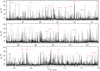 |
Fig. 4 Full final spectrum from 84 to 116 GHz. In red is reported the name of the molecular species associated to some of the most common or bright lines. |
3.2 Spectral analysis
The line identification and the fit to the C2H4O2 isomers have been obtained with the software XCLASS5 (eXtended CASA Line Analysis Software Suite – Möller et al. 2017), which makes use of the Cologne Database for Molecular Spectroscopy6 (CDMS, Müller et al. 2001, 2005) and Jet Propulsion Laboratory7 (JPL, Pickett et al. 1998) catalogs, via the Virtual Atomic and Molecular Data Centre (VAMDC, Endres et al. 2016). The spectroscopic data of acetic acid, from the work of Ilyushin et al. (2013), were introduced into the CDMS in May 2019 to perform the analysis presented in this work. A complete documentation of the spectroscopic works the entries of the catalogs for MF, AA, and GA are based on, is given in Appendix A. For each molecular species the software computes a synthetic spectrum assuming LTE (the software also allows non-LTE analysis) using as possible free parameters the excitation temperature, Tex, the total column density, Ntot, of the molecule, the line FWHM, Δv, the velocity of the source, VLSR, and the angular diameter of the source θs. The LTE assumption is justified by the high density of hot cores; in fact, from the column density of H2 derived in Sect. 3.1, a rough estimate of the volume density of the core is n ~108 cm−3. The line analysis can be done without subtracting the continuum, which can be simulated simultaneously with the line emission. The fitting procedure varies the free parameters to minimize the χ2 between theobserved spectrum and the synthetic one. It is possible to select the frequency ranges for the fit, which allows us to limit the fit to a selected number of transitions. In order to estimate the degree of contamination in the observed transitions of AA, GA, and MF, due to emission by other species, we performed a preliminary line identification across the whole spectrum. Starting from the molecules responsible for the brightest lines, we carried out an investigation to identify as many species that can potentially contribute to the observed spectrum as possible. For the species identified in this way, we adjusted the parameters of the synthetic spectra until a reasonable fit (by visual inspection) was obtained. This preliminary identification was used to identify the transitions of the isomers of C2 H4O2, and among them, the most unblended, with the intention to use them in the XCLASS fitting procedure.
We followed three rules to identify a transition of one of the 3 C2 H4O2 isomers: (i) the intensity of the line should be higher than 3 × rms; (ii) blending of a line of another species, with a separated peak, should start at a distance larger than FWHM/2 from the peak; (iii) in the case of blending with separation <FWHM/2, the intensity of the line of the other species should be <15 % of the peak. In the case of AA, whose lines are more affected by blending, we included also lines with one of the two wings blended up to 60% of the peak (with respect to the baseline). The MF spectrum presents 196 identified lines, with brightness temperatures up to ~ 70 K. These include both ground state and vibrationally excited v18 = 1 transitions, with upper state energies (Eu) between ~10 and ~ 400 K. For GA we detected 20 lines, with brightness temperatures up to ~28 K. All the transitions are in the ground vibrational state and have energies Eu between ~ 25 and ~ 190 K. Lastly, we identified 26 lines of AA, with brightness temperatures up to ~ 23 K. These are ground state and vibrationally excited v18 = 1 transitions, with energies Eu between ~25 and ~ 400 K. To compare the best fit physical parameters of the three species in a consistent way, we performed the fit by selecting the most unblended transitions with energies Eu < 250 K. This energy constraint was due to GA not presenting identified unblended transitions of higher upper state energy. Beltrán et al. (2018) found a decrease in Tex of methyl formate with distance from the core center from Tex ~ 497 K at the inner radius of 0.′′22 to Tex ~ 110 K at a radius of 1′′.32. From these data, the average value of Tex of MF inside the main core is ~250 K. Despite the presence of this gradient in Tex, we decided to perform a single temperature component analysis, to reduce the number of free parameters as much as possible. For each molecule we selected the lines for the fitting procedure choosing the most unblended transitions and balancing the presence of low Eu and high Eu transition, to avoid possible biases. For MF we selected 25 lines, for GA 12 and for AA 14. We calculated the optical depth τ0 at the center of all the identified lines (see Appendix B) using the values listed in Table 5 and we find that all transitions are optically thin (τ0 ≪ 1). The identified transitions of the three molecules are listed in Tables C.1–C.3, together with τ0. The transitions selected for the XCLASS fit are listed in boldface. As only exception to the Eu < 250 K constraint, we have included in the fit the transition 24(14, 11)A2 → 24(13, 12)A1 of AA, which has Eu = 266 K, because it is blended with other transitions of the same species with Eu = 80 K. During the fit, the continuum, from Eq. (2), the FWHM and VLSR of the selected species were kept fixed to the values found by a preliminary fit (in which single transitions were selected and all the parameters were free to vary), while Tex and Ntot were free to vary.
Parameters of the continuum baseline.
Parameter of the best fit and abundances for MF, AA, and GA.
4 Results
In the following, we analyze the best fit physical parameters obtained from the line fitting performed with XCLASS for the three different isomers. The results of the fit are given in Table 5, while in Figs. 5–7 the transitions used to constrain the fit for MF, AA, and GA are reported, with the synthetic spectra obtained using the best fit parameters overlaid on the data. The total spectrum with the synthetic spectra of the three isomers obtained using the best fit parameters is given in Appendix D. The errors on Tex and Ntot take into account a 12% error, from the rms of the continuum baseline determination (see Sect. 2.3). To determine the abundances of the molecules we used the value of the column densities inside the 1′′.2 beam, divided by the value of column density of H2 found in Sect. 3.1, extracted from the same area, considering a 20% uncertainty. Figure 8 shows the integrated maps of 8 of the most unblended transitions of MF, AA, and GA with different values of upper state energy Eu (from ~25 to ~ 200 K). As seen in this figure, the emission of MF, AA, and GA comes only from the HMC and has a nearly circular shape in all the emission maps. To obtain a mean value of diameter of the emitting region of each molecule, the eight maps of a given molecule are normalized with respect to the peak intensity and averaged together. The result is shown in Fig. 9. The imfit task from CASA was used to fit a 2D Gaussian to these maps and thus obtain an estimate of the angular diameters of the emission, reported in Table 3. The column densities of the three isomers have been derived assuming a beam filling factor of 1.
The decrease in the normalized flux (F∕Fpeak) in the emission maps, as a function of the radius from the peak R, is shown in Fig. 10 for the mean maps (bold lines) and for the eight selected transitions (indicated in Table 3) at different values of Eu. These data were obtained by averaging the normalized flux inside circular rings centered on the mean map peak. As shown in Fig. 10, the emission of MF is the most extended among the three isomers, while AA is the most compact, even if with a small difference with respect to GA. In addition, we performed the fit of AA and MF including also the most unblended transitions of high-energy (Eu > 250 K) and discuss the results in Sect. 4.4.
4.1 Methyl formate
For methyl formate, we found an excitation temperature of Tex = 221 ± 27 K, a column density of Ntot = (2.0 ± 0.4) × 1018 cm−2, and an abundance X = (2.0 ± 0.6) × 10−7. The Tex is consistent with 250 K, the mean temperature of MF in the main core calculated using the temperature gradient found by Beltrán et al. (2018). From the total spectrum in Appendix D, we see that there are transitions of MF (not used for the fit) that are under-reproduced by more than 20% by the best fit synthetic spectrum. About a third of these transitions are indeed blended with other molecular species, such as NS, CH3CN, 13 CH3CN, C2 H5CN, and more. The others are mostly low-energy transitions, which would be better reproduced by a lower temperature component of the fit. However, a two-temperature component fit does not properly converge and does not significantly improve the fit, either in terms of χ2 or of visual comparison with the observed spectrum. These transitions will likely be better reproduced by a fit that takes into account the temperature gradient observed by the previous study of Beltrán et al. (2018). However, this is beyond the scope of this paper. In addition, we cannot exclude that some of these transitions may also be blended with still unidentified molecular species since the preliminary line identification does not explain the totality of the transitions in the spectrum.
The mean value of column density of MF inside 1.′′1 from the data of Beltrán et al. (2018) is of ~1.5 × 1018 cm−2, which is consistent with our results. The column density derived by us differs by only a factor 2.5 from the value of 5 × 1018 cm−2 found by Rivilla et al. (2017) from IRAM 30m data, considering a source size of 1′′.7, and is also consistent with the estimateof 3.4 × 1018 cm−2 of Calcutt et al. (2014), when rescaled to the same source size of this work. The distance between the peak of the continuum emission and the MF emission is only 0′′.09, which is smaller than the pixel size (0.′′15).
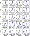 |
Fig. 5 Transitions used to fit methyl formate, with the LTE synthetic spectra simulated using the best fit parameters given in Table 5 in blue. |
4.2 Acetic acid
The best-fit parameters obtained with XCLASS for acetic acid are Tex = 299 ± 42 K, Ntot = (8.4 ± 1.4) × 1017 cm−2 and an abundance of X = (8 ± 3) × 10−8. The temperature is consistent within the errors with the mean temperature in the main core of ~ 250 K found from the relationship of Tex (MF) given in Beltrán et al. (2018). Nevertheless, the values of Tex for the three isomers cover a large range from ~130 to ~300 K (see Table 5). For this reason, to understand if the value of Tex of AA might be overestimated, we performed the fit to AA for a grid of fixed temperatures ranging from 100 K to 300 K. The only free parameter was the column density, Ntot. The results are given in Table 6 and shown in Fig. 11. From the plots it is possible to exclude Tex ≤ 150 K, but it is also clear that for seven transitions out of 14, there is a complete degeneracy between Tex and Ntot, for Tex ≥ 200 K. From this plot, we conclude that the excitation temperature of AA can be in the range 200-299 K (i.e., the value of best fit), leading to a range incolumn density of 4.3-8.4 × 1017 cm−2, with an uncertainty on Ntot of a factor ~2. This implies a range in abundance X between 4.3 × 10⁻⁸ and 8 × 10⁻⁸. The distance between the peak of the continuum emission and the AA emission is of 0′′.12, slightly larger with respect to MF but still smaller than the pixel size (0.′′15).
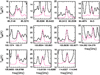 |
Fig. 6 Transitions used to fit acetic acid, with the LTE synthetic spectrum simulated using the best fit parameters given in Table 5 in pink. |
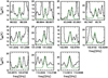 |
Fig. 7 Transitions used to fit glycolaldehyde, with the LTE synthetic spectra simulated using the best fit parameters given in Table 5 in green. |
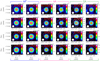 |
Fig. 8 Maps of integrated emission of 8 transitions with different Eu (from ~ 25 K to ~ 200 K) for MF (left panels), AA (middle panels) and GA (right panels) in color scale. Continuum emission is shown in withe contours, as in Fig. 2, and the beam is indicated in the left-bottom corner of the maps. |
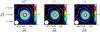 |
Fig. 9 Mean map for each molecule, obtained from the average of the 8 maps at different Eu in Fig. 8, rescaled to a peak of intensity 1 before averaging. The black dashed line is the contour where the emissionreaches the half the peak intensity. |
4.3 Glycolaldehyde
For GA, we found an excitation temperature of Tex = 128 ± 17 K, the lowest value for the three isomers, a column density of Ntot = (5.0 ± 0.7) × 1016 cm−2, and an abundance X = (5.0 ± 1.4) × 10−9. The low Tex can be due to the small number of detected transitions with Eu > 150 K (see Table B.3), and consequently the presence of only two high-energy transitions used for the fit, with Eu = 192 and 178 K, respectively. To understand if a higher Tex is compatible with the observed spectra, we performed the fit of GA for fixed values of Tex in the range 150 to 300 K, varying only the column density. The results of the fits are given in Table 7 and shown in Fig. 12. This figure shows that the transitions that are most sensitive to the value of Tex are those at frequency 93.048, 93.053 and 95.756 GHz. From the comparison of the spectra simulated and observed at these frequencies (Figs. 7 and 12), the best fit seems to be compatible with Tex ≤ 150 K, confirming the results of the XCLASS fit. The values of the column density found in G31 by Rivilla et al. (2017) and Calcutt et al. (2014) differ by a factor ~3.5 and ~0.8, respectively.The results for GA show the largest shift in position with respect to the peak of the continuum emission, with a distance of 0′′.22, which is still small compared to the angular resolution of the data.
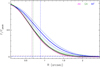 |
Fig. 10 Relative flux of emission maps shown in Figs. 8 (thin lines) and 9 (bold lines) as a function of R. The dashed vertical lines indicate the mean value between the two semiaxes of the elliptic 2D fit of the mean maps, calculated from the values given in Table 3. At these radii the emission of the mean maps differs slightly from 0.5 due to the fact that the fluxes plotted are calculated in circular rings, for simplicity. The horizontal dashed lines show the 3 × rms level for the mean emission maps. |
Ntot of the best fit for AA given a grid of fixed temperatures, with FWHM = 7.8 km s−1 and VLRS = 0.0 km s−1.
Ntot of the best fit for GA given a grid of fixed temperatures, with FWHM = 8.8 km s−1 and VLRS = 0.0 km s−1.
4.4 Methyl formate and acetic acid fit including Eu > 250 K
In Sects. 4.1 and 4.2, we reported the fit of MF and AA while taking into account only the most unblended transitions with Eu < 250 K. We imposedthis restriction to trace the same gas, with the same physical conditions, for all the three isomers. Thus, we did not include highenergy transitions (higher than the highest energy transition of GA available) that are, in principle, possibly emitted by a warmer gas. For completeness, we present the fit of AA and MF, including also the most unblended transitions of energy Eu > 250 K. We selected four transitions for AA ranging from 260 to 510 K, and 7 for MF ranging from 250 to 420 K, to add to the previously selected transitions for the fit. These new transitions are indicated by an asterisk in Tables C.1 and C.2.
The results of the new fit for AA are an excitation temperature Tex = 290 ± 40 K and a column density of Ntot = (8.0 ± 1.2) × 1017 cm−2, whereas for MF, we find Tex = 229 ± 28 K and a column density of Ntot = (2.1 ± 0.3) × 1018 cm−2. Based on a comparison with the values in Table 5, the results are very consistent within the errors. This indicates that for MF and AA in G31, even the highest energy transitions have the same excitation conditions as lower energy transitions and, thus, they are emitted by gas with the same physical conditions.
5 Discussion
5.1 Comparison with other sources
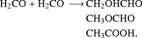
Figure 13 shows the abundances with respect to H2 (upper panel) and the column density ratios (lower panel) of the three isomers of C2 H4O2 in G31 and in the sources in literature for which all three isomers have been observed and at least two of them detected. The upper panel shows a very restricted sample, with respect to the lower panel, because it was for only four sources that we found an estimate of N(H2) on an angular scale comparable to the size of the region over which the column densities of the three isomers have been derived. The column density ratios, the abundances and the N(H2) adopted, and the corresponding references are given in Table 8. Here, G31 has the highest values of abundance of MF and AA among the four sources shown, with a difference of one and two orders of magnitude, respectively, from the second-highest values in the sample. The abundances in G31 are calculated using N(H2) = (1.0 ± 0.2) × 1025 cm−2 (see Sect. 3.1). Even considering this value as a lower limit – Rivilla et al. (2017) found a value four times larger – and adopting a value of one order of magnitude higher, the abundance of AA would still be the largest in the sample, at least one order of magnitude above the others. From the upper panel, a unique behavior for the three isomers in both high-mass and low-mass sources does not seem to exist. This is confirmed by the column density ratios in the extended sample shown in the lower panel.For IRAS 16293-2422A, Rivilla et al. (2019) found a column density of GA towards the peak one order of magnitude larger than the one in Table 8 and in Fig. 13 by Manigand et al. (2020). Manigand et al. (2020) selected an off-peak position to extract the spectrum, shifted by an amount comparable (by eye) with the emission size of AA and GA, thus possibly leading to underestimated values of these column densities.
The lower panel in Fig. 13 confirms the large fraction of acetic acid in G31, with respect to the extended sample. In fact, in only three sources (four including the lower limit in NGC 1333 IRAS 4A) MF/AA<10: G31, SgrB2(N), and the position “v” in NGC 6334I MM1. The column density ratios of the isomers are plotted in Fig. 14, which are useful for the search for possible correlations. The first plot (upper-left) does not show a clear correlation between MF/AA and MF/GA, however, despite the large scatter, a hint of the dual distribution that was first seen by El-Abd et al. (2019) in the space NMF - NGA is still visible. On the other hand, there seems to be an anti-correlation (Pearson’s χ2 = 0.73) between MF/AA and AA/GA (upper-right), where we can also possibly see the same dual distribution – although not as clearly – and a faint correlation (Pearson’s χ2 = 0.51) between MF/GA and AA/GA (lower panel), even though with some spread. The bimodal distribution is not driven by a difference between high-mass sources and low-mass sources, but the origin must be related to particular physical or chemical conditions inside some sources (both high-mass and low-mass), as already stated by El-Abd et al. (2019).
Lastly, from our work we derived the size of the emission of the three isomers, confirming a difference in the extension and showing as AA and GA are more compact than MF. This result is consistent with what shown in the maps towards other sources by Remijan et al. (2002), Jørgensen et al. (2016), Xue et al. (2019), El-Abd et al. (2019) and Manigand et al. (2020). Towards G31, AA shows the most compact emission among the three isomers.
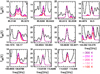 |
Fig. 11 Transitions used to fit acetic acid, with the LTE synthetic spectra simulated assuming different excitation temperatures, and leaving as free parameters only the column density. The value used are given in Table 6. |
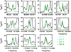 |
Fig. 12 Transitions used to fit glycolaldehyde, with the LTE synthetic spectra simulated assuming different excitation temperatures, and leaving as free parameters only the column density. The values we used are given in Table 7. |
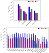 |
Fig. 13 Upper panel: abundances wrt H2 for the sources with an estimate in Table 8. For G31, the values of X(AA) given in the figure have been calculated from the mean value of the observed range in column density 4.3 × 10¹⁷−8.4 × 1017cm−2, while the error bars cover the entire range. For IRAS 16293 B, the value of N(H2) is a lower limit, leading to upper limits on the abundances, but not affecting the ratios between abundances. Lower panel: ratio of the column densities of the three isomers of C2 H4O2 for the sources listed in Table 8. For G31, the values of MF/AA and AA/GA have been calculated using the mean value of the observed range 4.3 × 10¹⁷−8.4 × 1017cm−2 for AA, while the error bars cover the ratios given by entire range. The sources labelled as MM1 i-viii and MM2 i-iii refer to NGC 6334I MM1, and NGC 6334I MM2, while the source labelled as NGC 1333 is NGC 1333 IRAS 4A. |
5.2 Comparison with chemical models and laboratory studies
For several years, the only efficient chemical pathways leading to the formation of the three isomers of C2 H4O2 were found to be on the surface of dust grains (Garrod & Herbst 2006; Garrod et al. 2008; Beltrán et al. 2009; Laas et al. 2011; Woods et al. 2012, 2013; Garrod 2013; Coutens et al. 2018; Rivilla et al. 2019). When temperatures are sufficiently high, radicals have enough energy to diffuse across the surface and react to form COMs. The main routes on warm dust grains for the formation of the three isomers from the aforementioned studies are:
 (4)
(4)
 (5)
(5)
 (6)
(6)
 (7)
(7)
 (8)
(8)
Laboratory studies have also investigated possible routes for the formation of MF and GA on the surface of dust grains at low temperatures (Fedoseev et al. 2015; Chuang et al. 2016), showing that the reactions can take place even at temperatures as low as ~10 K. This has also been confirmed by Simons et al. (2020) using microscopic kinetic Monte Carlo simulations to simulate ice chemistry. Nevertheless, the increase of temperature in more evolved sources, like G31, increases the mobility of radicals on the surface leading to higher efficiency of the routes (Eqs. (4)–(8)) than those proposed in the experiment at low temperatures.
Gas-phase chemical routes might be also efficient at low temperatures and, thus, capable of explaining the detection of COMs in a cold environment (Öberg et al. 2010; Bacmann et al. 2012; Jiménez-Serra et al. 2016). In the model by Vasyunin & Herbst (2013), the most efficient gas-phase pathway to the formation of MF in a cold environment (T ~ 10 K) is given by the radiative association reaction (Horn et al. 2004):
 (9)
(9)
followed by a dissociative recombination and an isomerization, that leads to the formation of MF. Balucani et al. (2015) proposed the following chain of reactions for the production of MF:
 (10)
(10)
 (11)
(11)
 (12)
(12)
 (13)
(13)
starting from the non-thermal desorption of methanol at low temperature. Vasyunin et al. (2017) included these new gas-phase reactions in their network to model abundances of complex organic species in the prestellar core L1544 including MF. Reaction (13) of the chain proposed by Balucani et al. (2015) is indeed themost efficient pathway for the formation of MF in this cold environment, accounting for two-thirds of the total production. Nevertheless, the production of the reactant CH3OCH2 is mainly dominated by the reaction studied by Shannon et al. (2014):
 (14)
(14)
rather than reaction (12), due to the low abundances of F and Cl. Approximately the remaining one third of total MF is generated by the ion-neutral reaction
 (15)
(15)
and the subsequent dissociative recombination of  . The abundances of COMs, such as MF, dimethyl ether, formamide, and acetaldehyde are of the order of 10−12−10−10, thus, gas-phase reactions can reproduce the observed abundances in cold low-mass objects. However, the abundance of MF derived in, for instance, L1544 or L1689B (Bacmann et al. 2012; Jiménez-Serra et al. 2016) is two to three orders of magnitude below that obtained for G31. Coutens et al. (2018) report that in their models for star-forming regions hosting a proto-star with mass from 1 to 60 M⊙ MF reaches abundances in the range 7 × 10⁻¹⁰−2.5 × 10⁻⁸, when the temperatures are high (100−300 K). These results are obtained with a network considering only gas-phase reactions for MF, including the ones in Balucani et al. (2015). They found that the peak of abundance of MF from gas-phase reactions only is a factor of two smaller than the value estimated in G31 by Rivilla et al. (2017), and the inclusion of route (4) on grain-surface is able to bridge this discrepancy. However, the new estimate presented in this work is a factor of five greater, implying that grain surface reactions are likely responsible for the majority of the abundance of MF detected in G31. Garrod (2013) found that reaction (4) can efficiently lead to abundances of ~ 1 × 10⁻⁷. From this, MF would behave in a similar way as other COMs such as formamide (see Quénard et al. 2018), whose production at low T is dominated by gas-phase chemistry, while its formation is governed by grain surface reactions in warm or hot sources such as hot corinos or hot cores.
For GA and AA, Skouteris et al. (2018) introduced a new chain of reactions that leads to the formation of these C2 H4O2 isomers:
 (16)
(16)
 (17)
(17)
 (18)
(18)
starting from the sublimation of ethanol in gas-phase. The GA abundance prediction of the model that simulates the chemistry in a hot corino, varies over a broad range ~ 10−10−10−8 and shows a strong dependence on the hydroxyl radical OH, on the rate coefficient of the reaction (16), and on the initial abundance of ethanol (CH3CH2OH). Assuming the most favorable rate coefficient and an abundance of ethanol of ~ 6 × 10⁻⁸ (wrt H2), the model of Skouteris et al. (2018) predicts an abundance of GA close to the one derived in this work, but the abundance of AA is about one order of magnitude lower than the new estimate towards G31. These values are derived before sublimated ethanol is fully consumed for a gas with temperature equal to 100 K and H nuclei density 2 × 108 cm−3. Nevertheless, Coutens et al. (2018) have shown that GA can efficiently form from reactions (6) and (8) on dust grains and reproduce the abundances in G31 observed by Rivilla et al. (2017) and the new estimate presented in this work. It must be noted that these calculations have been made assuming a mass of 25 M⊙ (from Osorio et al. 2009) for the proto-star embedded in G31, derived using the old estimates of distance of 7.9 kpc. The new estimate of the distance to G31, which affects the estimate of the mass and luminosity of the proto-star(s) embedded in G31, might lead to a change in the modeled abundances. Similarly to Coutens et al. (2018), Rivilla et al. (2019) have found that the main formation route for GA in IRAS 16293-2422 proto-stars is reaction (6), with possible contributions also from reaction (8). The formation of GA through grain-surface reactions in Rivilla et al. (2019) is strengthen by the fact that their grain-surface network reproduces both GA and that of its precursor HCO abundances.
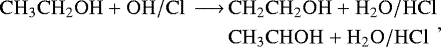
Unlike GA, the abundance of AA from gas-phase reactions as a function of ethanol abundance and the different rate coefficient possibilities is not given in Skouteris et al. (2018). If we assume that the ratio AA/GA ~ 10 (found in the aforementioned specific case of ethanol abundance ~6 × 10⁻⁸), is conserved, in principle the abundance of AA in this work could be covered by the wide range derived from multiplying for a factor 10 the given range ~10−10−10−8 of GA in Skouteris et al. (2018). However, this relies on many assumptions that need to be further tested. The observed abundance estimated this work cannot be reproduced with reaction (5) included in the chemical network of Garrod (2013). Further investigations of reaction (16) and of the abundance of ethanol in G31 is needed to constrain the formation route of AA in G31, which might also lead to completely discard the proposed gas-phase pathways (16)–(18).
The fact that the rate coefficients of reactions (17) and (18) have a dependence on temperature implies that both gas-phase and grain-surface reactions can possibly explain the more extended emission of MF with respect to AA and GA. In fact, the gas-phase reactions for AA and GA would be more efficient closer to the center of the core due to the increase in temperature. On the other hand, for grain-surface reactions, Burke et al. (2015) found that MF desorbs at lower temperature with respect to AA and GA, which follow the desorption of water ice. Recently, Ahmad et al. (2020) proposed a new pathway for the formation of the three isomers both in gas-phase and on grain surface, involving formaldehyde:
 (19)
(19)
All the three channels show high energy barriers that can be crossed thanks to quantum tunneling or thermal hopping. The study also reports that reaction (19), in all the three cases, is more efficient on grain-surface. However, no calculations have been made to predict the abundances that can be reached thanks to this pathway on grain surface in star-forming regions. Silva et al. (2020) simulated the channel of reaction (19) that leads to GA in the condition of a high-mass protostellar object in gas-phase, and the maximum abundance is of ~ 10−12, that is orders of magnitude below the value observed in G31 as well as SgrB2(N).
A summary of the reaction routes and the predictions of the different models is given in Table 9. In conclusion, for MF grain-surface reactions are likely responsible for its high abundance in G31. The results from GA and its precursor HCO in IRAS 16293-2422 A & B by Rivilla et al. (2019) could suggest a grain-surface formation for GA in hot sources like G31. However, the case of GA is not of straightforward interpretation as both gas-phase and grain-surface reactions could be at play considered the uncertainties in the chemical models aforementioned, and, as a results, both scenarios are able to explain the more compact morphology of GA with respect to MF. For AA, the routes included in Garrod (2013) are not able to reproduce the high-abundance found towards G31, while the gas-phase route proposed by Skouteris et al. (2018) could not be excluded and, rather, needs to be further tested in order to reduce the large uncertainties on their predictions. In case of any future discrepancy with the narrowed prediction of this route and the abundance found in G31, the main pathway(s) responsible for the high abundance of AA in G31 should be further investigated. Similarly to GA, both gas-phase and grain-surface reactions could explain the more compact morphology of AA with respect to MF.
Column density ratios between the 3 isomers of C2H4O2 and abundances from star-forming regions in this work and in literature.
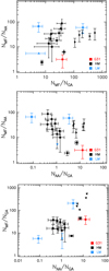 |
Fig. 14 Comparison of the ratios between the three isomers of C2H4O2 for the sources listed in Table 8. For G31, the values of MF/AA and AA/GA given in the figure are calculated using the mean value of the observed range 4.3 × 10¹⁷−8.4 × 1017cm−2 for AA, while the error bars have been estimated from the entire range. |
Summary of the chemical routes to the formation of the 3 isomers of C2 H4O2, and related reactions.
6 Conclusions
In this paper, we present the data of the GUAPOS survey, an unbiased spectral survey performed with ALMA towards G31.41+0.31, one of the most chemically rich HMC known, located outside the GC. The survey covered a ~ 32 GHz bandwidth with a spectral resolution of 0.488 MHz and an angular resolution of 1′′.2.
We detected, for the first time, all the three isomers of C2 H4O2 towards thisHMC. This increases the number of high-mass sources outside the GC, where the three isomers have been detected, to a total of three. The emission of all the isomers is compact towards the HMC and the most extended emission is from MF, while AA is the most compact. Here, MF is the most abundant of the isomers, confirming what has been seen in the other sources. Then, G31 shows the largest abundance of AA with respect to the other sources. From the comparison with the literature, it seems that a unique behavior of the three isomers does not exist both in high- and low-mass sources.
The comparison with chemical models suggests that the MF abundance found in G31 is not reproducible using only gas-phase routes, thus revealing the need for grain-surface reactions. On the other hand, the scenario for AA and GA does not have a straightforward interpretation. Both gas-phase and grain-surface reactions are able to reproduce the observed abundance of GA, with uncertainties. However, in the case of the gas-phase reactions proposed by Skouteris et al. (2018), the wide range of predicted abundances for GA is strictly related to the uncertainties in the reaction of CH3CH2OH with the hydroxyl radical, while the predictions from grain-surface reactions in Coutens et al. (2018) might be altered by the adoption of the new estimate of the distance to G31. For AA, the chemical model by Garrod (2013), including route (5) on grain-surface, is not able to reproduce the high abundance found in G31. On the other hand, the gas-phase route by Skouteris et al. (2018) should be further tested to reduce the uncertainties. Moreover, the more compact morphology of these two isomers with respect to MF can be explained in both scenarios (grain-surface and gas-phase) as well. To remove some of the uncertainties, laboratory and theoretical studies on reaction (16) are needed, together with an estimate of the abundance of the reactant CH3CH2OH in G31. If as a result, this route is not efficient enough to reproduce the abundance presented here, new formation routes should be investigated. To better understand and constrain whether the main chemical routes that lead to GA are in gas-phase or in grain-surface chemistry, or whether both reactions are necessary, a systematic study is needed, which would include the new routes by Skouteris et al. (2018), such as the one performed in Quénard et al. (2018) for formamide, in which the two types of chemistry were switched off alternatively.
Acknowledgements
The authors thank the referee Brett A. McGuire for the constructive comments which helped to improve the quality and readability of the paper. The authors wish to thank Holger S.P. Müller and Christian Endres for inserting acetic acid in the CDMS catalog. C.M. and L.C. acknowledge support from the Italian Ministero dell’Istruzione, Universitá e Ricerca through the grant Progetti Premiali 2012 – iALMA (CUP C52I13000140001). I.J.-S. has received partial support from the Spanish FEDER (project number ESP2017-86582-C4-1-R). V.M.R. has received funding from the European Union’s Horizon 2020 research and innovation programme under the Marie Skłodowska-Curie grant agreement No 664931. This paper makes use of the following ALMA data: ADS/JAO.ALMA#2017.1.00501.S. ALMA is a partnership of ESO (representing its member states), NSF (USA) and NINS (Japan), together with NRC (Canada), MOST and ASIAA (Taiwan), and KASI (Republic of Korea), in cooperation with the Republic of Chile. The Joint ALMA Observatory is operated by ESO, AUI/NRAO and NAOJ.
Appendix A Catalog entries documentation for the three isomers of C2 H4O2
A.1 Methyl Formate
The data set used in JPL catalog is based on Ilyushin et al. (2009) and includes data from Brown et al. (1975), Bauder (1979), Demaison et al. (1983), Plummer et al. (1984, 1986), Oesterling et al. (1999), Karakawa et al. (2001), Hitoshi et al. (2003), Ogata et al. (2004), Carvajal et al. (2007), Maeda et al. (2008b,a)8.
A.2 Acetic Acid
The data set used in the CDMS catalog is based on Ilyushin et al. (2013) and includes data from Krisher & Saegebarth (1971), van Eijck et al. (1981), Demaison et al. (1982, 1983), van Eijck & van Duijneveldt (1983), Wlodarczak & Demaison (1988), Ilyushin et al. (2001, 2003)9.
A.3 Glycolaldehyde
The data set used in JPL catalog is based on Marstokk & Møllendal (1970, 1973), Butler et al. (2001), Widicus Weaver et al. (2005), Carroll et al. (2010)10.
Appendix B Optical depth of the lines
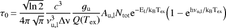
Equation (B.28) of Möller et al. (2017) gives the optical depth of a line as a function of frequency:
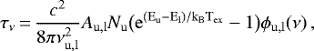 (B.1)
(B.1)
where c is the speed of light, νu,l is the frequency of the transition, Au,l is the Einstein’s coefficient of the transition, Nu is the column density of the molecule in the upper state of the transition, and Eu and El are the energy level of the upper and lower states of the transition and ϕu,l (ν) is the normalized line profile (i.e., ∫ ϕu,l(ν) dν = 1). Nu is related to the total column density of the molecule, Ntot, through the Boltzmann distribution,
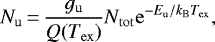 (B.2)
(B.2)
where gu is the degeneracy of the level u, Eu the corresponding and Q(Tex) the partition function of the molecular species, calculated at the temperature of excitation Tex. If we assume that τν has a Gaussian profile of the type
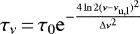 (B.3)
(B.3)
where τ0 is the opacity at the line center and Δν is the FWHM, then the integral of the optical depth over frequency will be related to the central opacity of the line by
 (B.4)
(B.4)
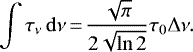
Integrating Eq. (B.1) on ν and using Eqs. (B.2) and (B.4) we obtain the espression for the optical depth at the center of the line
 (B.5)
(B.5)
where Δv is the FWHM in velocity units, namely Δv = Δν c∕νu,l.
Appendix C Tables of identified transitions
Tables C.1-C.3 are only available at the CDS.
Appendix D Full spectrum
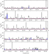 |
Fig. D.1 Total spectra of the GUAPOS project in black. In blue, we show the synthetic spectrum of the best fit of methyl formate (MF); in green the synthetic spectrum of the best fit of glycolaldehyde (GA); in pink the synthetic spectrum of the best fit of acetic acid (AA). The colored triangles indicate the transitions used to constrain the fitting procedure of the 3 different molecules. Closer views of those transitions are given in Figs. 5–7. |
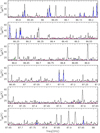 |
Fig. D.1 continued. |
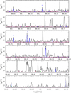 |
Fig. D.1 continued. |
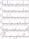 |
Fig. D.1 continued. |
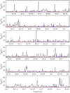 |
Fig. D.1 continued. |
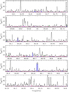 |
Fig. D.1 continued. |
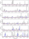 |
Fig. D.1 continued. |
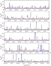 |
Fig. D.1 continued. |
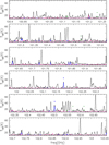 |
Fig. D.1 continued. |
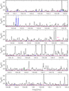 |
Fig. D.1 continued. |
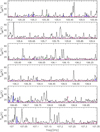 |
Fig. D.1 continued. |
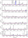 |
Fig. D.1 continued. |
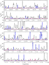 |
Fig. D.1 continued. |
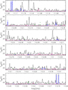 |
Fig. D.1 continued. |
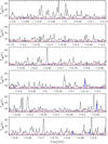 |
Fig. D.1 continued. |
References
- Ahmad, A., Shivani, Misra, A., & Tandon, P. 2020, Res. A&A, 20, 014 [Google Scholar]
- Araya, E., Hofner, P., Kurtz, S., Olmi, L., & Linz, H. 2008, ApJ, 675, 420 [NASA ADS] [CrossRef] [Google Scholar]
- Arce, H. G., Santiago-García, J., Jørgensen, J. K., Tafalla, M., & Bachiller, R. 2008, ApJ, 681, L21 [NASA ADS] [CrossRef] [Google Scholar]
- Bacmann, A., Taquet, V., Faure, A., Kahane, C., & Ceccarelli, C. 2012, A&A, 541, L12 [NASA ADS] [CrossRef] [EDP Sciences] [Google Scholar]
- Balucani, N., Ceccarelli, C., & Taquet, V. 2015, MNRAS, 449, L16 [Google Scholar]
- Bauder, A. 1979, J. Phys. Chem. Ref. Data, 8, 583 [NASA ADS] [CrossRef] [Google Scholar]
- Beckwith, S. V. W., & Sargent, A. I. 1991, ApJ, 381, 250 [NASA ADS] [CrossRef] [Google Scholar]
- Belloche, A., Müller, H. S. P., Menten, K. M., Schilke, P., & Comito, C. 2013, A&A, 559, A47 [NASA ADS] [CrossRef] [EDP Sciences] [Google Scholar]
- Belloche, A., Müller, H. S. P., Garrod, R. T., & Menten, K. M. 2016, A&A, 587, A91 [NASA ADS] [CrossRef] [EDP Sciences] [Google Scholar]
- Belloche, A., Garrod, R. T., Müller, H. S. P., et al. 2019, A&A, 628, A10 [NASA ADS] [CrossRef] [EDP Sciences] [Google Scholar]
- Beltrán, M. T., Cesaroni, R., Neri, R., et al. 2004, ApJ, 601, L187 [NASA ADS] [CrossRef] [Google Scholar]
- Beltrán, M. T., Cesaroni, R., Neri, R., et al. 2005, A&A, 435, 901 [NASA ADS] [CrossRef] [EDP Sciences] [Google Scholar]
- Beltrán, M. T., Codella, C., Viti, S., Neri, R., & Cesaroni, R. 2009, ApJ, 690, L93 [NASA ADS] [CrossRef] [Google Scholar]
- Beltrán, M. T., Cesaroni, R., Rivilla, V. M., et al. 2018, A&A, 615, A141 [NASA ADS] [CrossRef] [EDP Sciences] [Google Scholar]
- Beltrán, M. T., Padovani, M., Girart, J. M., et al. 2019, A&A, 630, A54 [CrossRef] [EDP Sciences] [Google Scholar]
- Beuther, H., Zhang, Q., Bergin, E. A., et al. 2007, A&A, 468, 1045 [NASA ADS] [CrossRef] [EDP Sciences] [Google Scholar]
- Bonato, M., Liuzzo, E., Giannetti, A., et al. 2018, MNRAS, 478, 1512 [NASA ADS] [CrossRef] [Google Scholar]
- Bottinelli, S., Ceccarelli, C., Williams, J. P., & Lefloch, B. 2007, A&A, 463, 601 [NASA ADS] [CrossRef] [EDP Sciences] [Google Scholar]
- Briggs, D. S. 1995, AAS Meeting Abstracts, 187, 112.02 [Google Scholar]
- Brown, R. D., Crofts, J. G., Gardner, F. F., et al. 1975, ApJ, 197, L29 [NASA ADS] [CrossRef] [Google Scholar]
- Burke, D. J., Puletti, F., Brown, W. A., et al. 2015, MNRAS, 447, 1444 [NASA ADS] [CrossRef] [Google Scholar]
- Butler, R. A. H., De Lucia, F. C., Petkie, D. T., et al. 2001, ApJS, 134, 319 [NASA ADS] [CrossRef] [Google Scholar]
- Calcutt, H., Viti, S., Codella, C., et al. 2014, MNRAS, 443, 3157 [NASA ADS] [CrossRef] [Google Scholar]
- Carroll, P. B., Drouin, B. J., & Widicus Weaver, S. L. 2010, ApJ, 723, 845 [NASA ADS] [CrossRef] [Google Scholar]
- Carvajal, M., Willaert, F., Demaison, J., & Kleiner, I. 2007, J. Mol. Spectr., 246, 158 [NASA ADS] [CrossRef] [Google Scholar]
- Cazaux, S., Tielens, A. G. G. M., Ceccarelli, C., et al. 2003, ApJ, 593, L51 [NASA ADS] [CrossRef] [Google Scholar]
- Cernicharo, J., Marcelino, N., Roueff, E., et al. 2012, ApJ, 759, L43 [NASA ADS] [CrossRef] [Google Scholar]
- Cesaroni, R. 2019, A&A, 631, A65 [CrossRef] [EDP Sciences] [Google Scholar]
- Cesaroni, R., Churchwell, E., Hofner, P., Walmsley, C. M., & Kurtz, S. 1994a, A&A, 288, 903 [NASA ADS] [Google Scholar]
- Cesaroni, R., Olmi, L., Walmsley, C. M., Churchwell, E., & Hofner, P. 1994b, ApJ, 435, L137 [NASA ADS] [CrossRef] [Google Scholar]
- Cesaroni, R., Hofner, P., Walmsley, C. M., & Churchwell, E. 1998, A&A, 331, 709 [Google Scholar]
- Cesaroni, R., Hofner, P., Araya, E., & Kurtz, S. 2010, A&A, 509, A50 [NASA ADS] [CrossRef] [EDP Sciences] [Google Scholar]
- Cesaroni, R., Beltrán, M. T., Zhang, Q., Beuther, H., & Fallscheer, C. 2011, A&A, 533, A73 [NASA ADS] [CrossRef] [EDP Sciences] [Google Scholar]
- Cesaroni, R., Sánchez-Monge, Á., Beltrán, M. T., et al. 2017, A&A, 602, A59 [NASA ADS] [CrossRef] [EDP Sciences] [Google Scholar]
- Chuang, K. J., Fedoseev, G., Ioppolo, S., van Dishoeck, E. F., & Linnartz, H. 2016, MNRAS, 455, 1702 [Google Scholar]
- Coletta, A., Fontani, F., Rivilla, V. M., et al. 2020, A&A, 641, A54 [CrossRef] [EDP Sciences] [Google Scholar]
- Coutens, A., Viti, S., Rawlings, J. M. C., et al. 2018, MNRAS, 475, 2016 [NASA ADS] [CrossRef] [Google Scholar]
- Csengeri, T., Belloche, A., Bontemps, S., et al. 2019, A&A, 632, A57 [NASA ADS] [CrossRef] [EDP Sciences] [Google Scholar]
- Demaison, J., Dubrulle, A., Boucher, D., Burie, J., & van Eijck, B. P. 1982, J. Mol. Spectr,, 94, 211 [NASA ADS] [CrossRef] [Google Scholar]
- Demaison, J., Boucher, D., Dubrulle, A., & Van Eijck, B. P. 1983, J. Mol. Spectr., 102, 260 [NASA ADS] [CrossRef] [Google Scholar]
- El-Abd, S. J., Brogan, C. L., Hunter, T. R., et al. 2019, ApJ, 883, 129 [CrossRef] [Google Scholar]
- Endres, C. P., Schlemmer, S., Schilke, P., Stutzki, J., & Müller, H. S. P. 2016, J. Mol. Spectr., 327, 95 [NASA ADS] [CrossRef] [Google Scholar]
- Favre, C., Carvajal, M., Field, D., et al. 2014, ApJS, 215, 25 [NASA ADS] [CrossRef] [Google Scholar]
- Fedoseev, G., Cuppen, H. M., Ioppolo, S., Lamberts, T., & Linnartz, H. 2015, MNRAS, 448, 1288 [NASA ADS] [CrossRef] [Google Scholar]
- Fontani, F., Pascucci, I., Caselli, P., et al. 2007, A&A, 470, 639 [NASA ADS] [CrossRef] [EDP Sciences] [Google Scholar]
- Galametz, M., Maury, A. J., Valdivia, V., et al. 2019, A&A, 632, A5 [NASA ADS] [CrossRef] [EDP Sciences] [Google Scholar]
- Garrod, R. T. 2013, ApJ, 765, 60 [Google Scholar]
- Garrod, R. T., & Herbst, E. 2006, A&A, 457, 927 [NASA ADS] [CrossRef] [EDP Sciences] [Google Scholar]
- Garrod, R. T., Widicus Weaver, S. L., & Herbst, E. 2008, ApJ, 682, 283 [NASA ADS] [CrossRef] [Google Scholar]
- Gibb, A. G., Wyrowski, F., & Mundy, L. G. 2004, ApJ, 616, 301 [NASA ADS] [CrossRef] [Google Scholar]
- Girart, J. M., Beltrán, M. T., Zhang, Q., Rao, R., & Estalella, R. 2009, Science, 324, 1408 [NASA ADS] [CrossRef] [PubMed] [Google Scholar]
- Herbst, E., & van Dishoeck, E. F. 2009, ARA&A, 47, 427 [NASA ADS] [CrossRef] [Google Scholar]
- Hitoshi, O., Kazumi, O., Kojiro, T., & Shozo, T. 2003, Molecules, 8 [Google Scholar]
- Hofner, P., & Churchwell, E. 1993, Astrophysical Masers (Berlin: Springer), 412, 164 [CrossRef] [Google Scholar]
- Hollis, J. M., Lovas, F. J., & Jewell, P. R. 2000, ApJ, 540, L107 [NASA ADS] [CrossRef] [Google Scholar]
- Hollis, J. M., Vogel, S. N., Snyder, L. E., Jewell, P. R., & Lovas, F. J. 2001, ApJ, 554, L81 [Google Scholar]
- Horn, A., Møllendal, H., Sekiguchi, O., et al. 2004, ApJ, 611, 605 [NASA ADS] [CrossRef] [Google Scholar]
- Ilyushin, V. V., Alekseev, E. A., Dyubko, S. F., et al. 2001, J. Mol. Spectr., 205, 286 [NASA ADS] [CrossRef] [Google Scholar]
- Ilyushin, V. V., Alekseev, E. A., Dyubko, S. F., & Kleiner, I. 2003, J. Mol. Spectr., 220, 170 [NASA ADS] [CrossRef] [Google Scholar]
- Ilyushin, V., Kryvda, A., & Alekseev, E. 2009, J. Mol. Spectr., 255, 32 [NASA ADS] [CrossRef] [Google Scholar]
- Ilyushin, V. V., Endres, C. P., Lewen, F., Schlemmer, S., & Drouin, B. J. 2013, J. Mol. Spectr., 290, 31 [NASA ADS] [CrossRef] [Google Scholar]
- Immer, K., Li, J., Quiroga-Nuñez, L. H., et al. 2019, A&A, 632, A123 [CrossRef] [EDP Sciences] [Google Scholar]
- Isokoski, K., Bottinelli, S., & van Dishoeck, E. F. 2013, A&A, 554, A100 [NASA ADS] [CrossRef] [EDP Sciences] [Google Scholar]
- Jacobsen, S. K., Jørgensen, J. K., Di Francesco, J., et al. 2019, A&A, 629, A29 [NASA ADS] [CrossRef] [EDP Sciences] [Google Scholar]
- Jiménez-Serra, I., Vasyunin, A. I., Caselli, P., et al. 2016, ApJ, 830, L6 [Google Scholar]
- Jørgensen, J. K., Favre, C., Bisschop, S. E., et al. 2012, ApJ, 757, L4 [NASA ADS] [CrossRef] [Google Scholar]
- Jørgensen, J. K., van der Wiel, M. H. D., Coutens, A., et al. 2016, A&A, 595, A117 [NASA ADS] [CrossRef] [EDP Sciences] [Google Scholar]
- Kalenskii, S. V., & Johansson, L. E. B. 2010, Astron. Rep., 54, 1084 [NASA ADS] [CrossRef] [Google Scholar]
- Karakawa, Y., Oka, K., Odashima, H., Takagi, K., & Tsunekawa, S. 2001, J. Mol. Spectr., 210, 196 [NASA ADS] [CrossRef] [Google Scholar]
- Krisher, L. C., & Saegebarth, E. 1971, J. Chem. Phys., 54, 4553 [NASA ADS] [CrossRef] [Google Scholar]
- Laas, J. C., Garrod, R. T., Herbst, E., & Widicus Weaver, S. L. 2011, ApJ, 728, 71 [NASA ADS] [CrossRef] [Google Scholar]
- Lykke, J. M., Favre, C., Bergin, E. A., & Jørgensen, J. K. 2015, A&A, 582, A64 [NASA ADS] [CrossRef] [EDP Sciences] [Google Scholar]
- Maeda, A., Medvedev, I. R., De Lucia, F. C., Herbst, E., & Groner, P. 2008a, ApJS, 175, 138 [NASA ADS] [CrossRef] [Google Scholar]
- Maeda, A., De Lucia, F. C., & Herbst, E. 2008b, J. Mol. Spectr., 251, 293 [NASA ADS] [CrossRef] [Google Scholar]
- Manigand, S., Jørgensen, J. K., Calcutt, H., et al. 2020, A&A 635, A48 [NASA ADS] [CrossRef] [EDP Sciences] [Google Scholar]
- Marstokk, K. M., & Møllendal, H. 1970, J. Mol. Struct., 5, 205 [NASA ADS] [CrossRef] [Google Scholar]
- Marstokk, K. M., & Møllendal, H. 1973, J. Mol. Struct., 16, 259 [NASA ADS] [CrossRef] [Google Scholar]
- Martín, S., Martín-Pintado, J., Blanco-Sánchez, C., et al. 2019, A&A, 631, A159 [NASA ADS] [CrossRef] [EDP Sciences] [Google Scholar]
- Mayen-Gijon, J. M., Anglada, G., Osorio, M., et al. 2014, MNRAS, 437, 3766 [NASA ADS] [CrossRef] [Google Scholar]
- McGuire, B. A., Burkhardt, A. M., Kalenskii, S., et al. 2018, Science, 359, 202 [Google Scholar]
- McMullin, J. P., Waters, B., Schiebel, D., Young, W., & Golap, K. 2007, ASP Conf. Ser., 376, 127 [Google Scholar]
- Mehringer, D. M., Snyder, L. E., Miao, Y., & Lovas, F. J. 1997, ApJ, 480, L71 [NASA ADS] [CrossRef] [Google Scholar]
- Möller, T., Endres, C., & Schilke, P. 2017, A&A, 598, A7 [NASA ADS] [CrossRef] [EDP Sciences] [Google Scholar]
- Müller, H. S. P., Thorwirth, S., Roth, D. A., & Winnewisser, G. 2001, A&A, 370, L49 [NASA ADS] [CrossRef] [EDP Sciences] [Google Scholar]
- Müller, H. S. P., Schlöder, F., Stutzki, J., & Winnewisser, G. 2005, J. Mol. Struct., 742, 215 [NASA ADS] [CrossRef] [Google Scholar]
- Öberg, K. I., Bottinelli, S., Jørgensen, J. K., & van Dishoeck, E. F. 2010, ApJ, 716, 825 [NASA ADS] [CrossRef] [Google Scholar]
- Oesterling, L. C., Albert, S., De Lucia, F. C., Sastry, K. V. L. N., & Herbst, E. 1999, ApJ, 521, 255 [NASA ADS] [CrossRef] [Google Scholar]
- Ogata, K., Odashima, H., Takagi, K., & Tsunekawa, S. 2004, J. Mol. Spectr., 225, 14 [NASA ADS] [CrossRef] [Google Scholar]
- Osorio, M., Anglada, G., Lizano, S., & D’Alessio, P. 2009, ApJ, 694, 29 [NASA ADS] [CrossRef] [Google Scholar]
- Ossenkopf, V., & Henning, T. 1994, A&A, 291, 943 [NASA ADS] [Google Scholar]
- Ott, S. 2010, ASP Conf. Ser., 434, 139 [Google Scholar]
- Pickett, H. M., Poynter, R. L., Cohen, E. A., et al. 1998, J. Quant. Spectr. Rad. Transf., 60, 883 [Google Scholar]
- Plummer, G. M., Herbst, E., De Lucia, F., & Blake, G. A. 1984, ApJS, 55, 633 [NASA ADS] [CrossRef] [Google Scholar]
- Plummer, G. M., Herbst, E., De Lucia, F. C., & Blake, G. A. 1986, ApJS, 60, 949 [NASA ADS] [CrossRef] [Google Scholar]
- Quénard, D., Jiménez-Serra, I., Viti, S., Holdship, J., & Coutens, A. 2018, MNRAS, 474, 2796 [NASA ADS] [CrossRef] [Google Scholar]
- Remijan, A., Snyder, L. E., Liu, S. Y., Mehringer, D., & Kuan, Y. J. 2002, ApJ, 576, 264 [NASA ADS] [CrossRef] [Google Scholar]
- Remijan, A., Snyder, L. E., Friedel, D. N., Liu, S. Y., & Shah, R. Y. 2003, ApJ, 590, 314 [NASA ADS] [CrossRef] [Google Scholar]
- Rivilla, V. M., Beltrán, M. T., Cesaroni, R., et al. 2017, A&A, 598, A59 [NASA ADS] [CrossRef] [EDP Sciences] [Google Scholar]
- Rivilla, V. M., Beltrán, M. T., Vasyunin, A., et al. 2019, MNRAS, 483, 806 [NASA ADS] [CrossRef] [Google Scholar]
- Sakai, Y., Kobayashi, K., & Hirota, T. 2015, ApJ, 803, 97 [CrossRef] [Google Scholar]
- Sánchez-Monge, Á., Schilke, P., Schmiedeke, A., et al. 2017, A&A, 604, A6 [NASA ADS] [CrossRef] [EDP Sciences] [Google Scholar]
- Sánchez-Monge, Á., Schilke, P., Ginsburg, A., Cesaroni, R., & Schmiedeke, A. 2018, A&A, 609, A101 [NASA ADS] [CrossRef] [EDP Sciences] [Google Scholar]
- Shannon, R. J., Caravan, R. L., Blitz, M. A., & Heard, D. E. 2014, Phys. Chem. Chem. Phys. 16, 3466 [CrossRef] [Google Scholar]
- Silva, S. G. S., Vichietti, R. M., Haiduke, R. L. A., Machado, F. B. C., & Spada, R. F. K. 2020, MNRAS, 497, 4486 [CrossRef] [Google Scholar]
- Simons, M. A. J., Lamberts, T., & Cuppen, H. M. 2020, A&A, 634, A52 [CrossRef] [EDP Sciences] [Google Scholar]
- Skouteris, D., Balucani, N., Ceccarelli, C., et al. 2018, ApJ, 854, 135 [Google Scholar]
- Taquet, V., López-Sepulcre, A., Ceccarelli, C., et al. 2015, ApJ, 804, 81 [NASA ADS] [CrossRef] [Google Scholar]
- van Eijck, B. P., & van Duijneveldt, F. B. 1983, J. Mol. Spectr., 102, 273 [NASA ADS] [CrossRef] [Google Scholar]
- van Eijck, B. P., van Opheusden, J., van Schaik, M. M. M., & van Zoeren, E. 1981, J. Mol. Spectr., 86, 465 [NASA ADS] [CrossRef] [Google Scholar]
- Vastel, C., Ceccarelli, C., Lefloch, B., & Bachiller, R. 2014, ApJ, 795, L2 [Google Scholar]
- Vasyunin, A. I., & Herbst, E. 2013, ApJ, 769, 34 [Google Scholar]
- Vasyunin, A. I., Caselli, P., Dulieu, F., & Jiménez-Serra, I. 2017, ApJ, 842, 33 [Google Scholar]
- Widicus Weaver, S. L., Butler, R. A. H., Drouin, B. J., et al. 2005, ApJS, 158, 188 [NASA ADS] [CrossRef] [Google Scholar]
- Wlodarczak, G., & Demaison, J. 1988, A&A, 192, 313 [NASA ADS] [Google Scholar]
- Woods, P. M., Kelly, G., Viti, S., et al. 2012, ApJ, 750, 19 [NASA ADS] [CrossRef] [Google Scholar]
- Woods, P. M., Slater, B., Raza, Z., et al. 2013, ApJ, 777, 90 [NASA ADS] [CrossRef] [Google Scholar]
- Xue, C., Remijan, A. J., Burkhardt, A. M., & Herbst, E. 2019, ApJ, 871, 112 [NASA ADS] [CrossRef] [Google Scholar]
- Ysard, N., Koehler, M., Jimenez-Serra, I., Jones, A. P., & Verstraete, L. 2019, A&A, 631, A88 [NASA ADS] [CrossRef] [EDP Sciences] [Google Scholar]
Webpage of the project: http://www.arcetri.astro.it/~guapos/
Madrid Data Cube Analysis (MADCUBA) is a software developed in the Center of Astrobiology (Madrid) to visualize and analyze data cubes and single spectra (Martín et al. 2019): https://cab.inta-csic.es/madcuba/
More information is available at https://spec.jpl.nasa.gov/ftp/pub/catalog/doc/d060003.pdf
More information is available at https://cdms.astro.uni-koeln.de/cdms/portal/catalog/1605/#
More information is available at https://spec.jpl.nasa.gov/ftp/pub/catalog/doc/d060006.pdf
All Tables
Ntot of the best fit for AA given a grid of fixed temperatures, with FWHM = 7.8 km s−1 and VLRS = 0.0 km s−1.
Ntot of the best fit for GA given a grid of fixed temperatures, with FWHM = 8.8 km s−1 and VLRS = 0.0 km s−1.
Column density ratios between the 3 isomers of C2H4O2 and abundances from star-forming regions in this work and in literature.
Summary of the chemical routes to the formation of the 3 isomers of C2 H4O2, and related reactions.
All Figures
|
Fig. 1 Chemical structures of the three isomers of C2H4O2. |
| In the text | |
|
Fig. 2 Continuum map of the HMC G31.41+0.31 and the nearby UC HII region. Contour levels are at 5, 10, 20, 40, 60, 100, and 200 times the value of rms = 0.8 mJy beam−1. The three white triangles indicate the coordinates of the Main Core and NE core by Beltrán et al. (2018), and of the UC HII region by Cesaroni et al. (1998). The beam is shown in white in the lower left corner. |
| In the text | |
|
Fig. 3 Graphic scheme of the steps followed to obtain the final spectrum. |
| In the text | |
|
Fig. 4 Full final spectrum from 84 to 116 GHz. In red is reported the name of the molecular species associated to some of the most common or bright lines. |
| In the text | |
|
Fig. 5 Transitions used to fit methyl formate, with the LTE synthetic spectra simulated using the best fit parameters given in Table 5 in blue. |
| In the text | |
|
Fig. 6 Transitions used to fit acetic acid, with the LTE synthetic spectrum simulated using the best fit parameters given in Table 5 in pink. |
| In the text | |
|
Fig. 7 Transitions used to fit glycolaldehyde, with the LTE synthetic spectra simulated using the best fit parameters given in Table 5 in green. |
| In the text | |
|
Fig. 8 Maps of integrated emission of 8 transitions with different Eu (from ~ 25 K to ~ 200 K) for MF (left panels), AA (middle panels) and GA (right panels) in color scale. Continuum emission is shown in withe contours, as in Fig. 2, and the beam is indicated in the left-bottom corner of the maps. |
| In the text | |
|
Fig. 9 Mean map for each molecule, obtained from the average of the 8 maps at different Eu in Fig. 8, rescaled to a peak of intensity 1 before averaging. The black dashed line is the contour where the emissionreaches the half the peak intensity. |
| In the text | |
|
Fig. 10 Relative flux of emission maps shown in Figs. 8 (thin lines) and 9 (bold lines) as a function of R. The dashed vertical lines indicate the mean value between the two semiaxes of the elliptic 2D fit of the mean maps, calculated from the values given in Table 3. At these radii the emission of the mean maps differs slightly from 0.5 due to the fact that the fluxes plotted are calculated in circular rings, for simplicity. The horizontal dashed lines show the 3 × rms level for the mean emission maps. |
| In the text | |
|
Fig. 11 Transitions used to fit acetic acid, with the LTE synthetic spectra simulated assuming different excitation temperatures, and leaving as free parameters only the column density. The value used are given in Table 6. |
| In the text | |
|
Fig. 12 Transitions used to fit glycolaldehyde, with the LTE synthetic spectra simulated assuming different excitation temperatures, and leaving as free parameters only the column density. The values we used are given in Table 7. |
| In the text | |
|
Fig. 13 Upper panel: abundances wrt H2 for the sources with an estimate in Table 8. For G31, the values of X(AA) given in the figure have been calculated from the mean value of the observed range in column density 4.3 × 10¹⁷−8.4 × 1017cm−2, while the error bars cover the entire range. For IRAS 16293 B, the value of N(H2) is a lower limit, leading to upper limits on the abundances, but not affecting the ratios between abundances. Lower panel: ratio of the column densities of the three isomers of C2 H4O2 for the sources listed in Table 8. For G31, the values of MF/AA and AA/GA have been calculated using the mean value of the observed range 4.3 × 10¹⁷−8.4 × 1017cm−2 for AA, while the error bars cover the ratios given by entire range. The sources labelled as MM1 i-viii and MM2 i-iii refer to NGC 6334I MM1, and NGC 6334I MM2, while the source labelled as NGC 1333 is NGC 1333 IRAS 4A. |
| In the text | |
|
Fig. 14 Comparison of the ratios between the three isomers of C2H4O2 for the sources listed in Table 8. For G31, the values of MF/AA and AA/GA given in the figure are calculated using the mean value of the observed range 4.3 × 10¹⁷−8.4 × 1017cm−2 for AA, while the error bars have been estimated from the entire range. |
| In the text | |
|
Fig. D.1 Total spectra of the GUAPOS project in black. In blue, we show the synthetic spectrum of the best fit of methyl formate (MF); in green the synthetic spectrum of the best fit of glycolaldehyde (GA); in pink the synthetic spectrum of the best fit of acetic acid (AA). The colored triangles indicate the transitions used to constrain the fitting procedure of the 3 different molecules. Closer views of those transitions are given in Figs. 5–7. |
| In the text | |
|
Fig. D.1 continued. |
| In the text | |
|
Fig. D.1 continued. |
| In the text | |
|
Fig. D.1 continued. |
| In the text | |
|
Fig. D.1 continued. |
| In the text | |
|
Fig. D.1 continued. |
| In the text | |
|
Fig. D.1 continued. |
| In the text | |
|
Fig. D.1 continued. |
| In the text | |
|
Fig. D.1 continued. |
| In the text | |
|
Fig. D.1 continued. |
| In the text | |
|
Fig. D.1 continued. |
| In the text | |
|
Fig. D.1 continued. |
| In the text | |
|
Fig. D.1 continued. |
| In the text | |
|
Fig. D.1 continued. |
| In the text | |
|
Fig. D.1 continued. |
| In the text | |
Current usage metrics show cumulative count of Article Views (full-text article views including HTML views, PDF and ePub downloads, according to the available data) and Abstracts Views on Vision4Press platform.
Data correspond to usage on the plateform after 2015. The current usage metrics is available 48-96 hours after online publication and is updated daily on week days.
Initial download of the metrics may take a while.