| Issue |
A&A
Volume 644, December 2020
|
|
|---|---|---|
| Article Number | A73 | |
| Number of page(s) | 29 | |
| Section | Astrophysical processes | |
| DOI | https://doi.org/10.1051/0004-6361/202038867 | |
| Published online | 02 December 2020 | |
Jiamusi pulsar observations
III. Nulling of 20 pulsars⋆
1
National Astronomical Observatories, Chinese Academy of Sciences, Jia-20 Datun Road, ChaoYang District, Beijing 100101, PR China
e-mail: This email address is being protected from spambots. You need JavaScript enabled to view it.
, This email address is being protected from spambots. You need JavaScript enabled to view it.
2
CAS Key Laboratory of FAST, NAOC, Chinese Academy of Sciences, Beijing 100101, PR China
3
School of Astronomy, University of Chinese Academy of Sciences, Beijing 100049, PR China
4
The State Key Laboratory of Astronautic Dynamics, Xi’an, Shaanxi 710043, PR China
5
Jiamusi Deep Space Station, China Xi’an Satellite Control Center, Jiamusi, Heilongjiang 154002, PR China
6
Qiannan Normal University for Nationalities, Duyun, Guizhou 558000, PR China
Received:
8
July
2020
Accepted:
21
September
2020
Abstract
Aims. Most pulsar nulling observations have been conducted at frequencies lower than 1400 MHz. We aim to understand the nulling behaviors of pulsars at relatively high frequencies, and to decipher whether or not nulling is caused by a global change in the pulsar magnetosphere.
Methods. We used the Jiamusi 66 m telescope to observe 20 bright pulsars at 2250 MHz with unprecedented lengths of time. We estimated the nulling fractions of these pulsars, and identified the null and emission states of the pulses. We also calculated the nulling degrees and scales of the emission-null pairs to describe the distributions of emission and null lengths.
Results. Three pulsars, PSRs J0248+6021, J0543+2329, and J1844+00, are found to null for the first time. The details of null-to-emission and emission-to-null transitions within the pulse window are observed for the first time for PSR J1509+5531, which is a low-probability event. A complete cycle of long nulls with timescales of hours is observed for PSR J1709−1640. For most of these pulsars, the K-S tests of nulling degrees and nulling scales reject the hypothesis that null and emission are caused by random processes at high significance levels. Emission-null sequences of some pulsars exhibit quasi-periodic, low-frequency or featureless modulations, which might be related to different origins. During transitions between emission and null states, pulse intensities have diverse tendencies for variation. Significant correlations are found between respectively nulling fraction, nulling cadence, and nulling scale and the energy loss rate of the pulsars. Combined with the nulling fractions reported in the literature for 146 nulling pulsars, we find that statistically large nulling fractions are more tightly related to pulsar period than to characteristic age or energy-loss rate.
Key words: pulsars: general
The pulse sequences of all pulsars are available at the CDS via anonymous ftp to cdsarc.u-strasbg.fr (130.79.128.5) or via http://cdsarc.u-strasbg.fr/viz-bin/cat/J/A+A/644/A73 and at http://zmtt.bao.ac.cn/psr-jms/
© ESO 2020
1. Introduction
Pulse profiles obtained by integrating tens of thousands of individual pulses are generally stable and represent a unique feature of each pulsar. However, individual pulses vary considerably in intensity and phase. For some pulsars, the pulse-by-pulse emission suddenly ceases and no radio emission can be detected, but after some periods (one to a few thousand) the emission is restored and the pulsar can be detected again. This phenomenon is called nulling and was first reported by Backer (1970). To date, 214 pulsars have been reported to null (e.g., Ritchings 1976; Biggs 1992; Wang et al. 2007; Gajjar et al. 2012; Basu et al. 2017), which is less than 10% of the known pulsars. The actual number of nulling pulsars may be more because observations are restricted by sensitivity and the length of observation sessions.
Pulsars may null over a wide range of timescales from one rotation to many hours and even as long as months. The most prevalent nulls last for just a single period, such as for example that of PSR B2021+51, which is generally considered as a stochastic process within the pulsar magnetosphere (e.g., Basu et al. 2017). Long nulls of PSR B1706−16 last for 2−5 h (Naidu et al. 2018), which might be related to changes in plasma processes within a pulsar magnetosphere. Nulling for much longer timescales of days to months has been found for intermittent pulsars, such as PSR B1931+24 (Kramer et al. 2006), which is closely related to the spin-down energy loss.
To quantify the degree of nulling of a pulsar, the nulling fraction, fn, has been used to describe the percentage of periods with no detectable emission (Ritchings 1976), which varies from about zero to more than 90% (e.g., Naidu et al. 2018). Nulling pulsars with a similar nulling fraction may have quite different nulling lengths (Gajjar et al. 2012). It is not clear if nulling is a random phenomenon. The nonrandomness of nulls suggests that the emission or null of a pulse is not independent of the state of the preceding pulse. The nonrandomness assumption can be tested either by the Waled-Wolframite statistic or using the Kolmogorov-Smirnov (K-S) test (e.g., Redman & Rankin 2009). Gajjar et al. (2012) argued that the occurrence of nulls is not random based on the statistics of the distributions of null lengths, but speculated that the duration of nulls is random. We believe that both the occurrence and duration of nulls should be tested for correlations or randomness. If the nulling of a pulsar is not random, could it be modulated by periodic processes? Some attempts were made in previous studies and the periodic nulling was identified for pulsars like PSR B1133+16 (Herfindal & Rankin 2007; Basu et al. 2017). Nulling degree and nulling scale were introduced by Yang et al. (2014) to represent the angle in a rectangular coordinate for the numbers of nulls and emission,  , and their square length,
  . A null–emission pair with a nulling degree of 45° means that the nulls and emission are of similar length on average within the nulling cycle, and a nulling degree of ∼0° or 90° means that a pulsar has no nulling or is dominated by nulling, respectively.
Despite the global features of nulling, a zoomed-in view of transitions between emission and nulls exhibits diverse variations. Pulse emission generally begins abruptly, but can either decay exponentially to the nulling state, such as in the case of for example PSR B0818−41 (Bhattacharyya et al. 2010), or cease abruptly, which is the case for PSR B0031−07 for example (Gajjar et al. 2014a). Alternatively, for pulsars like PSR J1727−2739, the transitions from emission to null can be either rapid or gradual (Wen et al. 2016). These features of nulling might be related to a failure to generate particles near the pulsar polar cap region, to a loss of coherence for emissions (Filippenko & Radhakrishnan 1982), to a change of emission mechanism (Zhang et al. 1997), or to the geometry of view (Herfindal & Rankin 2007).
Sensitive single-pulse observations with long observation times are needed to improve our understanding of pulsar nulling. But most of the previous observations were carried out at frequencies lower than 1400 MHz. Nulling behaviors at high frequencies may be different, because emission at high frequencies originates from the low altitude in the magnetosphere where relativistic particles responsible for the emission would be different from those for the low-frequency emission (e.g., Wang et al. 2013). Nulling observations at high frequencies can be used to verify the broadband feature and distinguish if nulling is physical or geometrical in origin and whether or not it is caused by global changes in the magnetosphere of a pulsar.
In this paper, we investigate the nulling behaviors of 20 pulsars from very long-duration pulsar observations carried out at 2250 MHz using the Jiamusi 66 m telescope. This paper is organized as follows. In Sect. 2, we briefly describe the observation details and data-reduction procedures. Nulling analysis methods and nulling behaviors of individual pulsars are presented in Sect. 3. Discussion and conclusions are given in Sect. 4.
2. Observations and data reduction
Observations of 20 pulsars were carried out using the Jiamusi 66 m telescope at Jiamusi Deep Space Station, China Xi’an Satellite Control Center from 2015 June to 2018 September. The receiver used for observations has a central frequency of 2250 MHz and a bandwidth of about 140 MHz. Intermediate-frequency signals of left- and right-hand polarization were sampled, channelized, and added together with a digital backend. Data products from the Jiamusi 66 m telescope generally have 256 spectral channels with a frequency resolution of 0.58 MHz and a time resolution of 0.2 ms, or 128 spectral channels with a frequency resolution of 1.16 MHz and a time resolution of 0.1 ms. More details can be found in Han et al. (2016).
Offline data processing was carried out as follows. The total power is first scaled with respect to flux-calibrator observations (e.g., 3C286, 3C48) for each frequency channel. The data are then de-dispersed and binned to form single pulses for each frequency channel according to the ephemeride of a pulsar with DSPSR (van Straten & Bailes 2011). Radio frequency interference (RFI) is then identified and excised from a 2D frequency and time domain through statistical analysis of off-pulse and whole-pulse intensities with PSRCHIVE (Hotan et al. 2004). Further, the dynamic spectra are formed from the data to estimate the influence of interstellar scintillation by following Wang et al. (2018). We note that most of the observations are affected by interstellar scintillation due to small dispersion measures (DMs), and decorrelation bandwidths of the scintillation of these pulsars are larger than or comparable to the observation bandwidth of 140 MHz. To reduce its influence on our results, only the scintillation-enhanced blocks of data are chosen for this nulling analysis.
Observational parameters of the 20 pulsars are listed in Table 1. The number of frequency channels Nch and time duration for each observation Tobs in minutes are listed in Cols. 5 and 6. For weak pulsars, consecutive 2n pulses are integrated. The number of subintegrations Nsub is listed in Col. 7 with the number of Nint (2n) pulses integrated in each subintegration indicated in Col. 8. If one data section is affected by broad-band RFIs or faded by interstellar scintillation, these corrupted data blocks are omitted. The number of total data blocks Nblk is listed in Col. 9. Plots of pulse sequences are presented in Appendix A and indicated in Col. 10.
Observational parameters of 20 pulsars.
An example of pulse sequences is shown in Fig. 1 for PSR J1709−1640, with some apparently long nulls. A long block of scintillation-enhanced data is chosen for the nulling analysis, as demonstrated in the middle and left plots.
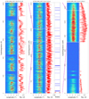 |
Fig. 1. Example of pulse sequence taken on 27 Oct 2017 for PSR J1709−1640. Left plots: part of the observation displayed with single pulses. Left panel: is for intensities of successive pulses. Right panel: is for the significance of on pulse (red) and off pulse (blue) emissions for each pulse. Middle plots: a much longer part of the observation taken for nulling analysis. The subintegrations are formed every two pulses, with its emission (1) or null (0) state indicated. Right plots: entire observation with subintegrations formed every 16 pulses. |
3. Nulling analysis
3.1. Emission-null sequences and nulling fraction
The emission and null states of pulsars are analyzed in a few steps. Although most of the intense RFIs have already been excised in a previous data-processing step, some pulsars are still affected by low levels of RFI. To get a flat baseline, we perform a least square fit of a fifth-order polynomial to the off-pulse regions for each subintegration, and subtract them from the data. An off-pulse window with the same number of bins (nbins) as the on-pulse window is selected. The significance of emission from both the on- and of-pulse windows is calculated for each subintegration:
 (1)
(1)
Here, σ is the standard deviation of off-pulse emission, Weq is the equivalent width of a top-hat pulse with the same area and peak height as the pulse profile integrated from all the subintegrations. The significance sequences are obtained for both the on and off pulses, which are then binned to form the histogram distributions. The distribution of off-pulse significance can be well modeled by a normal function with a mean of zero, an amplitude of A0, and a standard deviation of σoff:
 (2)
(2)
Any excess outside of this distribution for the on-pulse significance indicates that some pulses are in a nulling state. We fit the normal function with a mean of zero and a standard deviation σoff to the on-pulse distribution with significances less than zero to obtain the amplitude A1. The ratio is termed the nulling fraction fn = A1/A0, which has an uncertainty of
 (3)
(3)
Here, δA0 and δA1 represent the uncertainties obtained from the fitting. The scaled off-pulse distribution with fn is then subtracted from the distribution of on-pulse significance. The residual distribution generally follows a lognormal distribution,
![Mathematical equation: $$ \begin{aligned} D_{\rm on} (x)= \frac{B_0}{x} \exp \left[-\frac{(\ln x-\mu _{\rm on})^2}{2 \sigma _{\rm on}^2} \right], \end{aligned} $$](/articles/aa/full_html/2020/12/aa38867-20/aa38867-20-eq6.gif) (4)
(4)
where μon and σon are the mean and standard deviation of the normally distributed logarithm of the on-pulse significance. The value 3σoff represents the upper limit for the distribution of off-pulse significance. If exp(μon − 3σon) > 3σoff, then the pulses in the emission and null states are separated. The estimated fn represents a real fraction of pulses in nulling states. If exp(μon − 3σon) < 3σoff, the distributions for the emission and null pulses cannot be separated. The obtained fn is then overestimated, which represents an upper limit. When the possible short nulls are ignored, every 2n pulses are integrated for the pulse sequence until exp(μon − 3σon) > 3σoff. The fn obtained in this way represents a lower limit.
An example analysis of the nulling fraction is shown in Fig. 2 for PSR J0908−1739. The distribution of on-pulse significance is much broader, the lower three-sigma limit of which, exp(μon − 3σon), is smaller than 3σoff. The nulling pulses around zero are not well separated from the emission pulses, and the estimated fn of 29.2% represents an upper limit. In the bottom panels, every 32 pulses are integrated to improve the significance of pulses. The histograms for subintegrations with significance around zero are separated from those for the emission ones. The estimated fn = 18.8% represents a lower limit, because nulls shorter than 32 pulses cannot be resolved.
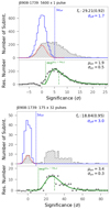 |
Fig. 2. Histograms of the significance of on-pulses (gray hatched step) and off-pulses (blue no hatched step) for PSR J0908−1739 taken on 23 May 2016. The upper plots are for statistics of single pulses, and the lower plots are for subintegrations of every 32 pulses. The distribution of the off-pulse significance can be modeled with a normal function with a mean of zero and a standard deviation of σoff. The normal function is scaled with fn and represented by a red dotted line; it is subtracted from the distribution of on-pulse significance with the residuals indicated by black “plus” symbols in the panel. The residual distribution is modeled by a lognormal function with a mean of μon and a standard deviation of σon. Green solid, dash-dotted, and dashed lines are for the modeled distribution, the mean, and the lower three-sigma limit. |
It should be noted that nulling fractions can be estimated either from the distributions of on and off pulse energy (e.g., Ritchings 1976; Gajjar et al. 2012) or from the distributions of their significance (Lynch et al. 2013). In previous studies, the on and off pulse energies were generally scaled by averages of energies for every 200 pulses to compensate for energy variation caused by interstellar scintillation, following Ritchings (1976). For long nulls (e.g., PSR J1709−1640), such robust correction biases the off-pulse energy distribution from the Gaussian, as noted by Vivekanand (1995). Identification of the emission or null state of a pulse or subintegration is often based on artificially setting a threshold significance, such as for example S/N = 3. If the energy distribution has a σoff > 1, the threshold S/N = 3 is not enough to discriminate the emission and null states. Our identification is based on the distribution of pulse significance with the following criteria:
(1) Any pulse with Son ≥ 4σoff is classified as an emission state;
(2) Any pulse with Son ≤ 2σoff is classified as a null for non-detection;
(3) If a pulse is of 2 σoff < Son ≤ 3σoff and the adjacent following and preceding pulses have Son > 3σoff, it is classified as an emission state, otherwise a null;
(4) If a pulse has 3 σoff < Son < 4σoff and the adjacent pulses have Son < 3σoff, it is classified as a null, otherwise an emission state.
The identified emission or null state for the example pulse sequence of PSR J1709−1640 is also shown in Fig. 1 with diverse nulling behaviors. The left and middle panels of the observation represent the normal states of the pulsar, which usually stays in an on state with short nulls of several to several tens of pulses. However, occasionally, the pulsar shows long nulls, as shown in the right panel of a long null of 6368 pulses for ∼1.2 h. Moreover, the sequence shows moderate nulls of 640 and 560 pulses before it goes into the long null, similar to those observed by Naidu et al. (2018).
Using this approach, we analyzed nulling fractions and states of 20 pulsars, as shown in Fig. B.1 and listed in Col. 3 of Table 2, with the number of pulses or subintegrations employed for the analysis listed in Col. 2. For five PSRs, namely J0332+5434, J1509+5531, J1932+1059, J2022+5154, and J2313+4253, the fn are obtained because their distributions of on- and off-pulse significance are separated with single pulses. For the other pulsars, only upper and lower limits of fn are estimated. The upper limits are obtained with single pulses whose distributions of on- and off-pulse significance are not resolved, and the lower limits are obtained with subintegrations with the separated distributions of on- and off-pulse significance. The cumulative probability, Pcri, for the modeled on-pulse distribution at 3σoff is calculated, as listed in Col. 4 in Table 2, which is the probability of misidentification of emission as null for the resolved on- and off-pulses or subintegrations.
Nulling statistics of 20 pulsars.
3.2. Emission and null lengths
The emission and null lengths represent the durations where a pulsar remains continuously at a given state. An emission–null (1–0) sequence is composed of interchanging emission and null states with lengths of (Ne1, Nn1, Ne2, Nn2, Ne3, ...). The number of state-changing cycles, Nc, is listed in Col. 5 of Table 2 for each pulsar. Its ratio, Nc/Nsub, represents the nulling cadence during one observation. Distributions of emission and null lengths vary significantly; their means, ⟨Ne⟩ and ⟨Nn⟩, together with standard deviations given in parentheses are listed in Cols. 6 and 7 of Table 2. Previously, it was suggested that emission and null states tend to be of short duration (to have small lengths) and exponential functions were usually employed to model both distributions (e.g., Gajjar et al. 2012).
The duration of an emission state might be related to the length of its prior or post nulls. From one emission–null sequence, the emission and the next null length pairs [(Ne1, Nn1), (Ne2, Nn2), ...], named EN, can be formed together with the emission and the pre-null length pairs [(Ne2, Nn1), (Ne3, Nn2), ...], named NE. As introduced by Yang et al. (2014), interaction between the states of emission and null can be demonstrated in terms of nulling degrees, α1 and α2, and nulling scales, s1 and s2, which correspond to emission and null length pairs from EN and NE. Their means and the standard deviations given in parentheses are listed in Cols. 8−11 of Table 2.
An example of the distributions of emission and null lengths is shown in Fig. 3 for PSR J1709−1640, with length pairs of EN and NE represented by red “o” symbols and blue crosses in the 2D length plan (bottom left). Histograms for the emission and null lengths are shown in the top and right panels and do not follow exponential functions. Figure 4 shows the distributions of nulling degrees and scales for both the EN and NE length pairs of PSR J1709−1640. It is apparent from the distribution of nulling degrees that nulls can have variable portions within a nulling cycle, but more cycles tend to have small nulling degrees. There are more cycles tending to have small nulling scales, but the distribution of these does not decay exponentially with the scale length.
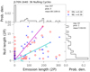 |
Fig. 3. Distributions of emission and null lengths of PSR J1709−1640. Pairs for the emission and the following null are denoted EN and are represented by red “o” symbol, while pairs for the emission and the pre-null are denoted NE and are represented by blue crosses. Nulling degrees, α1 and α2, and nulling scales, s1 and s2, are indicated for EN and NE. The correlation coefficients between emission and null lengths are shown in the top right corner. Histograms for the emission and null lengths are drawn in the top and right panels. Lengths of the longest emission or null state and their most probable and mean values are indicated in each panel. |
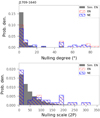 |
Fig. 4. Histograms of nulling degrees and nulling scales of emission–null length pairs of PSR J1709−1640. The left hatched red step and right hatched blue step represent distributions for the EN and NE length pairs, respectively. The gray bars are for the EN length pairs of randomly distributed emission–null sequence from simulation. |
We used this approach to analyze the emission and null lengths for 10 of the 20 pulsars that have well-distinguished emission and null states, as listed in Table 2 and shown in Fig. B.2. A few pulsars have dominant emission states and nulls generally last for short durations; for example, PSRs J1932+1059 and J2022+5154. The nulling degrees are in the range from about 1.4 to 26.3°. The nulling scales can have lengths from 27 to 353 pulses with comparable deviations. For most pulsars, the distributions of emission and null lengths cannot be well modeled by the exponential functions for the stochastic Poisson processes except for the emission lengths of PSRs J1509+5531 and J1932+1059.
3.3. Interactions between emission and null
For nulling pulsars, it was intuitively thought that the duration of an emission state might be dependent on the duration of the preceding nulling state, or vice versa. We examined correlations between the emission and null lengths, and correlation coefficients are listed in Cols. 2 and 3 of Table 3 for the EN and NE length pairs. The correlation coefficients for EN vary from −0.04 to 0.62 with a pair number weighted average of 0.03. While for NE length pairs, the coefficients vary from −0.14 to 0.36 with a weighted average of 0.07. This means that the duration of an emission or null state can be correlated with the duration of its preceding null or emission for some pulsars, but only with a marginal significance.
Results for correlations and randomness tests.
To further quantify the difference between the EN and NE, two sample K-S tests are carried out for both the nulling degrees (α1 vs. α2) and nulling scales (s1 vs. s2). Here, the tests are performed on the unbinned nulling degrees and scales, which return p-values and the statistic deviatives that represent the maximum difference of cumulative-distribution functions from α1 and α2, and those from s1 and s2, as listed in Cols. 4 and 7 of Table 3. If a p-value is larger than the significance level 0.1, the hypothesis that length pairs of EN and NE come from the same distribution cannot be rejected. For ten of the 20 pulsars with Nc > 10, the aforementioned statistics and K-S tests were performed. The K-S tests of α1 versus α2 of the ten pulsars have p-values larger than 0.51, this is much larger than the significance level of 0.1. The p-values of those tests of s1 versus s2 are larger than 0.71, which is also larger than the significance level. In summary, no significant difference is found between EN and NE length pairs from the distributions of α and s. Both the EN and NE may come from the same processes.
3.4. Randomness tests
To examine whether or not the emission and null interact randomly, the following statistical analysis was carried out. A sequence with the same size as observations of a pulsar is first simulated from a uniform distribution [0, 1). A threshold of nulling fraction is then set to the sequence; any value below that is denoted as null and vice visa for those above the threshold. The EN and NE length pairs are extracted from the simulated 1−0 sequence. If observations of a pulsar have more than 10 000 subintegrations or pulses, 1000 sets of randomly distributed 1−0 sequences are simulated to give average estimates for αs and ss. Otherwise, 10 000 sets of sequences are simulated for the estimation. From the EN and NE length pairs of these simulated sequences, nulling degrees and scales are calculated, which are termed as  ,
,  ,
,  , and
, and  .
.
Two sample K-S tests are taken on the observed and simulated sequences for α1 versus  and α2 versus
  for the occurrence of nulls. The statistic deviative and p-values are listed in Cols. 5 and 6 of Table 3 for the EN and NE length pairs. The same is done for s1 versus
  and s2 versus
  to test the duration of nulling cycles, as listed in Cols. 8 and 9 of Table 3. The simulated distributions are shown in Fig. 4 as an example and in Fig. B.2 for the ten pulsars.
(1) For the occurrence of nulls, the randomness hypothesis is rejected at high significance levels (p-values smaller than 0.1) for nine pulsars in Table 3 from both EN and NE except for PSR J0304+1932.
(2) For the duration of nulling cycles, the randomness hypothesis is rejected at high significance levels (p-values smaller than 0.1) for all ten of the pulsars from both EN and NE.
In summary, emission and null do not interact randomly for the occurrence and duration of the nine pulsars. The occurrence of a null can be random but its duration is not random for PSR J0304+1932.
3.5. Nulling periodicity
Blocks of emission and null pulses are generally arranged in a certain order within a sequence, some of which show quasi-periodic variations, as demonstrated in Fig. 1. To quantify this quasi-periodic pattern, a Fourier transform was performed on the emission–null (1–0) time sequence instead of the sequence for the total intensity. This is because the method concentrates only on the states of emission and eliminates the periodicities caused by subpulse drifting (e.g., Herfindal & Rankin 2007; Basu et al. 2017), mode-changing (e.g., Yan et al. 2020), and amplitude modulations (e.g., Basu et al. 2020). The discrete Fourier transformation (DFT) length depends on the length of an observation, which is chosen to ensure that the sequence has more than or equal to two but less than four DFT lengths. For a given sequence, the DFT process repeats by sliding 8, 16, or 32 points until the end. The power of all the DFTs from all the observations of a pulsar are finally averaged to form the entire spectra.
The DFT of the state sequence of one observation of PSR J1709−1640 is shown in Fig. 5 as an example. It is apparent that the 1−0 sequence is modulated across a broad range of periods. There might be a significant periodicity for part of the sequence, but it could be averaged out for the whole sequence and lead to the most probable modulations of about 200 periods. The 1−0 sequences of the ten pulsars show three kinds of periodic modulations, as shown in Fig. B.3:
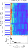 |
Fig. 5. Sliding Fourier transform of the emission–null (1–0) sequence for PSR J1709−1640. The emission or null state of each subintegration is indicated in the left panel. Discrete Fourier transformation power from a box car of 1024 points is plotted in the main panel, which slides across the state sequence every 32 points. The average power is shown in the bottom panel. |
(1) Four PSRs J0304+1932, J1509+5531, J1709−1640, and J2313+4253 have quasi-periodic nulling, with nulling frequencies listed in Col. 2 of Table 4. These behaviors might be related to the carousel beam patterns, and the nulls represent empty passes of sight lines through the patterns (e.g., Herfindal & Rankin 2007).
Nulling periodicity and intensity variations of ten pulsars.
(2) Emissions of PSRs J1239+2453, J2022+5154, and J2048−1616 are modulated by nulls with long periodicities, and the modulation is very strong for PSR J2321+6024. These pulsars occasionally exhibit frequent nulls, which might result from a change of pulsar emission mechanism. This can be caused either by a failure of particle production in the polar cap region of a pulsar magnetosphere or by loss of coherence for the relativistic particles (e.g., Filippenko & Radhakrishnan 1982; Zhang et al. 1997).
(3) PSRs J1136+1551 and J1932+1059 tend to have featureless modulations, that is, with a “white spectrum”. These pulsars null at a wide range of pulsar periods with no preferred periodicities.
3.6. Variation of pulse intensity during emission
Pulse intensities vary during an emission state. For emission states lasting for more than or equal to five pulses or subintegrations, the pulse intensity sequences are first normalized by the averages and sequence lengths, and then averaged across the normalized length. Systematic variation of pulse intensities, if it exists, should be revealed. Integrated pulse profiles are also obtained for the first, the second, and the last two subintegrations of emission on states, labeled E1, E2, E−2, and E−1, respectively. Intensity ratios, ⟨I2⟩/⟨I1⟩, for E2 to E1, and ⟨I−1⟩/⟨I−2⟩ for E−1 with respect to E−2, are listed in Cols. 2 and 3 of Table 4.
The tendencies of intensity variations for the emission states are shown in Fig. 6 for PSRs J1709−1640 and J2313+4253 as examples. PSR J2313+4253 is representative of most pulsars; its pulse intensity increases abruptly from a null at the beginning and diminishes quickly to null at the end, and the intensities of these pulses vary little during emission states. PSR J1709−1640 exceptionally rises to a higher intensity than the average at the start of the emission state, and gradually diminishes to null at the end.
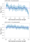 |
Fig. 6. Tendency of pulse intensity variation during the emission states for PSRs J1709−1640 and J2313+4253, normalized by its average intensity and emission length. Black dots with error bars represent the average pulse intensity. |
Variations of pulse shapes and intensities during the transitions from emission to null states and vice versa are shown in Fig. B.4. For PSRs J0304+1932, J1239+2453, J2048−1616, and J2321+6024, the first two subintegrations, E1 and E2, and the last two subintegrations, E−2 and E−1, are weaker than the average. For PSRs J1136+1551, J1932+1059, and J2022+5154, these pulses near the transitions are stronger than the average. PSRs J1709−1640 and J1509+5531 show exceptional transitions, as demonstrated in Fig. 7. The intensities of E1 and E2 of PSR J1709−1640 are stronger than the average, and E2 is even stronger than E1, but intensities of E−2 and E−1 are weaker than the average with E−1 weaker than E−2. Null-to-emission transition of PSR J1509+5531 starts with the leading component of the pulse profile emerging first, and emission-to-null transition also takes place first with the leading component, as shown in Fig. 8 for the four transitions. The phase dependency of transitions between emission and null implies that nulling of the pulsar is not caused by a global change of pulsar magnetosphere, but just by density patch changes of relativistic particles in parts of a magnetosphere.
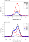 |
Fig. 7. Pulse profiles of PSRs J1709−1640 and J1509+5531 for the emission and nulls are represented by the thick solid and thin solid lines in black. Pulse profiles for the first and second subintegrations of the emission on states, E1 and E2, are represented by dashed lines in red, and those for the last and penultimate subintegrations, E−1 and E−2, are represented by dash-dotted lines in blue. |
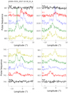 |
Fig. 8. Pulse sequences for the emission state setup (E1 − E4) and the transition to null (E−4 to E−1) for PSR J1509+5531. Null pulses are represented by the solid black lines. |
3.7. Notes for individual pulsars
3.7.1. PSR J0034–0721
PSR J0034−0721 is a famous pulsar with remarkable intensity and phase modulations. Its nulling state was first noticed by Huguenin et al. (1970). The nulls typically lasted for several tens to hundreds of periods, comparable with the duration of the emission states. There was at least one null separating two modes with different drifting rates (Smits et al. 2005; Ilie et al. 2020). Its nulling was found to be simultaneous across a broad range of frequencies (Gajjar et al. 2014b), with nulling fractions estimated to be 43% at 303 MHz (Gajjar et al. 2014b), 44.6% at 326.5 MHz (Vivekanand 1995), 31.3% at 333 MHz (Basu et al. 2017), 44% at 607 MHz (Gajjar et al. 2014b), 22.8% at 618 MHz (Basu et al. 2017), 37.7% at 645 MHz Biggs (1992), and 43% at 1380 MHz (Gajjar et al. 2014b). A periodicity of 75 rotations for the nulling was identified (Basu et al. 2017).
We made a long observation of 200 min at 2250 MHz, and integrated every 32 pulses to form subintegrations, as shown by two blocks of data in Fig. A.1. The nulling fraction is estimated to be in the range of 12.4% to 37.4%, which is consistent with the low-frequency estimates at 333 and 618 MHz, but smaller than those from Vivekanand (1995) and Gajjar et al. (2014b). The discrepancy is caused by the fact that their nulling fractions were estimated using extreme values instead of the total intensities of the pulses.
3.7.2. PSR J0248+6021
This is the first time that nulling is reported for this pulsar. Every 32 pulses are integrated to form subintegrations for two observations of 33 and 120 min, respectively, as shown in Fig. A.2. The nulling fraction is estimated to be in the range of 0.0% to 34.7%, as estimated from subintegrations of every 32 pulses and single pulses.
3.7.3. PSR J0304+1932
The pulse emission of PSR J0304+1932 is modulated by drifting subpulses and nulls. Its nulling fraction was found to be 13% and 14% from observations taken at 327 MHz (Redman & Rankin 2009; Herfindal & Rankin 2009), 8.7% at 333 MHz (Basu et al. 2017), 10% at 430 MHz (Rankin 1986), and 6.1% at 618 MHz (Basu et al. 2017). The nulling is not random (Redman & Rankin 2009), and has a periodicity of 128 ± 32 or 103 ± 34 rotations (Herfindal & Rankin 2009; Basu et al. 2017).
We made one observation at 2250 MHz for 56 min; every eight pulses are integrated to separate the emission and null pulses, as shown in Fig. A.3. PSR J0304+1932 typically nulls for about 16 pulses, and an estimated nulling fraction is in the range between 8.9% and 17.5%, consistent with those at low frequencies. Occurrence of its nulling is random, but the duration is not random as shown by the distributions of nulling scales, confirming the Wald-Wolfowitz run test results by Redman & Rankin (2009). Quasi-periodic modulation of about 90 rotations is marginally found, which agrees with the findings of Herfindal & Rankin (2009) and Basu et al. (2017).
3.7.4. PSR J0332+5434
The nulling of PSR J0332+5434 was first reported by Ritchings (1976) with a nulling fraction below 0.25% at 408 MHz. We made two observations for 180 and 84 min at 2250 MHz. Only two pulses may null among the 22 000 periods, as shown in Figs. A.4 and A.5. Hence, its nulling fraction is about 0%, consistent with the low frequency estimation.
3.7.5. PSR J0528+2200
PSR J0528+2200 has drifting and nulling behaviors, with nulling fractions of about 25% and 28% at 327 MHz (Herfindal & Rankin 2009; Redman & Rankin 2009), 14.4% at 333 MHz (Basu et al. 2017), and 25% at 610 MHz (Ritchings 1976). The nulls are not random (Redman & Rankin 2009), with two bright, probably harmonically related low-frequency structures as shown by Herfindal & Rankin (2009).
We made two observations for 29 and 32 min at 2250 MHz; every four pulses are integrated to form subintegrations. The significance distributions for the on- and off-pulses remain inseparable, as shown in Fig. A.6. The nulling fraction is estimated to be in the range of 8.1% to 22.3%, which is roughly consistent with those at low frequencies listed in Table C.1.
3.7.6. PSR J0543+2329
The nulling reported here is the first for this pulsar. We made two observations for 50 and 255 min at 2250 MHz. Every 16 pulses are folded to form subintegrations, as shown in Figs. A.7 and A.8. The nulling fraction is estimated to be in the range of 0.0% to 16.6%.
3.7.7. PSR J0826+2637
The nulling of PSR J0826+2637 was first found by Ritchings (1976) and was not random (Redman & Rankin 2009). The nulling fraction was estimated to be 7% at 327 MHz (Herfindal & Rankin 2009), but ≤5 at 430 MHz (Ritchings 1976). Recently, the prominent “quiet” and “bright” modes were identified, which might be related to the change of the plasma formation front (e.g., Sobey et al. 2015; Rankin et al. 2020). In the bright mode, the nulls had a fraction of a few percent, but more than 90% in the quiet mode (Basu & Mitra 2019).
We made three long observations at 2250 MHz, from which continuous blocks of pulses that are RFI-free and scintillation-enhanced (they might also be bright modes) are chosen for the nulling analysis. Every four pulses are integrated to form subintegrations, as shown in Figs. A.9–A.11. The lower and upper limits for the nulling fraction are estimated to be 0.0% and 3.4% from the entire 4745 subintegrations, which agrees with those at low frequencies for the bright mode, see Table C.1.
3.7.8. PSR J0908–1739
The nulling fraction of PSR J0908−1739 was found to be 26.8% at 333 MHz and 25.7% at 618 MHz (Basu et al. 2017). We made one observation for 37.4 min at 2250 MHz, and integrated every 32 pulses to form 175 subintegrations. The two significant nulls are shown in Fig. A.12. The nulling fraction is estimated to be in the range of 18.8% to 29.2%, consistent with those at low frequencies listed in Table C.1.
3.7.9. PSR J0922+0638
A nulling fraction below 0.05% was roughly estimated for PSR J0922+0638 at 430 MHz (Weisberg et al. 1986). We made three observations at 2250 MHz; every two pulses are folded, as shown in Figs. A.13 and A.14. The lower and upper limits of the nulling fraction are estimated to be 0.0% and 0.06%, respectively, from a total of 9600 subintegrations, consistent with those at low frequencies in Table C.1.
3.7.10. PSR J0953+0755
This pulsar has interpulse emission with a nulling fraction below 5% at 326.5 and 430 MHz (Ritchings 1976; Vivekanand 1995). We made one observation for 198 min at 2250 MHz; every eight pulses are integrated to form 5850 subintegrations, as shown in Fig. A.15. The lower and upper limits of the nulling fraction are estimated to be 0.1% and 11.8%, consistent with those at low frequencies in Table C.1.
3.7.11. PSR J1136+1551
Quasi-periodic intensity modulations were found for this bright pulsar (Taylor & Huguenin 1971), and the nulling was identified by Backer (1970). The nulling fractions are about 20% at 327 MHz (Bhat et al. 2007; Redman & Rankin 2009; Herfindal & Rankin 2009), 13.7% at 333 MHz (Basu et al. 2017), 14% at 408 MHz (Ritchings 1976) and 11.9% at 618 MHz (Basu et al. 2017). One of the double components of PSR J1136+1551 was missed at certain times, and the pulsar was otherwise noted as being partially nulling (Herfindal & Rankin 2009). The nulling is not random (Redman & Rankin 2009), and has a periodicity of about 30 rotations (Herfindal & Rankin 2007). Multi-frequency observations showed that the nulls do not always occur simultaneously; some pulses simply null at low frequencies (Bhat et al. 2007).
We made three observations at 2250 MHz. The second observation was affected by RFI and was split into four continuous blocks. Every four pulses of the observations are folded to form subintegrations, as shown in Figs. A.16–A.18. The nulling fraction is estimated to have a lower limit of 0.3% and an upper limit of 11.5%, roughly consistent with those at low frequencies. The occurrence and duration of nulls are not random, confirming the tests at low frequencies, but no significant periodicity of nulling is found, which means that the physical origins for its nulling should be frequency dependent.
3.7.12. PSR J1239+2453
PSR J1239+2453 is also among the first set of pulsars reported to null (Backer 1970). The amplitudes of its individual components were found to have different modulations (Taylor & Huguenin 1971), together with mode changing and sub-pulse drifting at multiple drift rates (e.g., Weltevrede et al. 2006; Naidu et al. 2017). The nulling fraction was estimated to be 7% at 325 MHz (Naidu et al. 2017), 6% at 327 MHz (Herfindal & Rankin 2009), 2% at 333 MHz (Basu et al. 2017), 6% at 408 MHz (Ritchings 1976), 4% at 610 MHz (Naidu et al. 2017), and 3.1% at 618 MHz (Basu et al. 2017). Observations at 325 and 610 MHz show that pulses null simultaneously at these two frequencies (Naidu et al. 2017), but no periodicity was found for the nulling (Basu et al. 2017).
We made four observations at 2250 MHz; every two pulses are integrated to form subintegrations, as shown in Figs. A.19 and A.20. Each observation demonstrates significant normal and abnormal states. The abnormal emissions are relatively strong, and are less affected by nulling. The most prevalent nulls are one or two pulses with a nulling fraction estimated to be in the range of 1.1% to 2.8%. The nulling fraction is consistent with those at 333 and 618 MHz from Basu et al. (2017). Fourier spectra of the emission-null sequences do not show any significant periodicity, which agrees with Basu et al. (2017).
3.7.13. PSR J1509+5531
The nulling of PSR J1509+5531 was first reported by Naidu et al. (2017) from simultaneous observations at 327 and 610 MHz, with a nulling fraction of 7% at 610 MHz. We made one long observation at 2250 MHz. To avoid RFI and interstellar scintillation, two blocks of single pulse data were chosen for the nulling analysis, as shown in Fig. A.21. Nulls occur for one or two pulses, with a nulling fraction estimated to be 2.0%, which is smaller than those at low frequencies. The profile components are not synchronous for null-to-emission and emission-to-null transitions, with the leading component emerging and diminishing first. The nulls are not random, and have a periodicity of about 23 rotations.
3.7.14. PSR J1709–1640
The nulling of this pulsar was first reported by Weltevrede et al. (2007). It usually stays in an active state with short nulls of less than 150 pulses. The nulling fraction is 3.7% at 333 MHz and 4.9% at 618 MHz (Basu et al. 2017). Occasionally, PSR J1709−1640 switches to an inactive state for long nulls of 1 to 4.7 h (Naidu et al. 2018). The nulls are found to be concurrent between 327 and 610 MHz.
We carried out a long observation of 220 min at 2250 MHz, which shows nulls for short (∼0.01 h), moderate (∼0.1 h), and long (∼1.2 h) durations; see Fig. A.22. Details of its nulling behaviors are discussed in Sect. 3. The nulling fraction is 35.6% for the whole dataset, but in the given scintillation-enhanced and RFI-free data this fraction is only between 2.1% and 3.4%, consistent with those at low frequencies in the active state. The nulls are not random, and have a periodicity of about 200 rotations.
3.7.15. PSR J1844+00
The nulling reported here is the first for this pulsar. We made one observation for 180 min at 2250 MHz; every 32 pulses are integrated to form subintegrations, as shown in Fig. A.23. Significant nulls of 256 pulses are detected. Its nulling fraction is estimated to be in the range between 0.3% and 34.0%.
3.7.16. PSR J1932+1059
PSR J1932+1059 has an interpulse, and was first reported to null by Backer (1970), with a nulling fraction below 1% at 408 MHz (Ritchings 1976). We made one long observation for 275 min at 2250 MHz, and data are separated into four blocks to avoid RFI, as shown in Figs. A.24 and A.25. PSR J1932+1059 typically nulls for one pulse and the duration of emission roughly follows exponential distributions. Its nulling fraction is estimated to be 0.03%, consistent with the low-frequency one. The occurrence and duration of nulls are not random. Its average emission remains stable and no nulling periodicity is found.
3.7.17. PSR J2022+5154
The nulling of PSR J2022+5154 was first reported by Ritchings (1976). The nulls generally last for one or two periods with a nulling fraction below 5% at 408 MHz (Ritchings 1976), or 1.4% at 610 MHz (Gajjar et al. 2012). We made three observations at 2250 MHz, as shown in Figs. A.26 and A.27. PSR J2022+5154 typically nulls for one pulse with a nulling fraction of 0.12%, consistent with that at 408 MHz but smaller than that at 610 MHz. The occurrence and duration of nulls are not random, but no periodicity of nulling can be identified.
3.7.18. PSR J2048–1616
The fluctuation of the three components of PSR J2048–1616 was investigated by Taylor & Huguenin (1971), which revealed sub-pulse drifting and nulling. The nulls were found to be broad band (Naidu et al. 2017) with a nulling fraction of 14% at 325 MHz (Naidu et al. 2017), 10% at 326.5 MHz (Vivekanand 1995), 8.3% at 333 MHz (Basu et al. 2017), 10% at 408 MHz (Ritchings 1976), 17% at 610 MHz (Naidu et al. 2017), 9.0% at 618 MHz (Basu et al. 2017) but 22% at 1308 MHz (Naidu et al. 2017). These nulls showed periodic variations of about every 51 rotations (Basu et al. 2017).
We made two observations for 30 and 300 min at 2250 MHz. The longer observation was seriously affected by RFI, and only one block of 116 pulses was chosen for the analysis. Every two pulses of the observations are folded, as shown in Fig. A.28. The nulls usually last for less than five pulses with a nulling fraction in the range between 2.1% and 6.4%, which is smaller than those at low frequencies. The nulls of PSR J2048−1616 are not random, but no significant periodicity is identified for the nulling.
3.7.19. PSR J2313+4253
PSR J2313+4253 was reported to null with a nulling fraction of 3.7% at 333 MHz by Basu et al. (2017), and the nulls have a periodicity of about every 32 rotations. We made one observation at 2250 MHz. Two blocks of data were chosen for the nulling analysis, as shown in Fig. A.29. PSR J2313+4253 typically nulls for one pulse with a nulling fraction of 5.2%, which is slightly larger than that at low frequency. Fourier spectra analysis demonstrates that the emission of PSR J2313+4253 is modulated by nulls with a periodicity of about 45 rotations, which agrees with the low-frequency measurement in Table C.1.
3.7.20. PSR J2321+6024
The frequent nulls of PSR J2321+6024 were first reported by Ritchings (1976), which correlated with the drifting and the mode-changing (Wright & Fowler 1981). The nulling fraction is about 35% at 303 MHz (Gajjar et al. 2014b), 25% at 408 MHz (Ritchings 1976), 33% at 607 MHz (Gajjar et al. 2014b), 29% at 610 MHz (Gajjar et al. 2012), 31% at 1380 MHz, and > 30% at 4850 MHz (Gajjar et al. 2014b). Simultaneous observations by Gajjar et al. (2014b) showed that the nulls were highly concurrent across a broad frequency range, and 1−3% of the pulses deviate from this behavior.
We made two observations for 5 and 7 h. The first observation and four blocks of the second observation were chosen for the nulling analysis, as shown in Figs. A.30–A.32. PSR J2321+6024 frequently nulls with a nulling fraction in the range between 8.5% and 18.5%, smaller than those previous estimates by about 30%. This is because the less significant emitting pulses cannot be modeled by the significance distributions of off-pulses, as shown by the excess of the residual distribution in Fig. B.1, but previous studies termed these as nulls. These nulls are not random, and the emission are modulated by nulls at long periodicities.
4. Discussion and conclusions
In this paper, we investigate the nulling behaviors of 20 pulsars by employing single-pulse observations at 2250 MHz made using the JMS 66 m telescope. This is the first time that nulling is reported for three pulsars, PSRs J0248+6021, J0543+2329, and J1844+00. A set of consistent methods is proposed for nulling analysis. The nulling fractions are first estimated for these pulsars at relatively high frequency. The emission-null (1–0) sequences are then constructed from which the emission and null lengths, their interactions, randomness, and the periodicity are analyzed.
In general, the distributions of emission and null lengths cannot be well modeled by exponential functions for most of the pulsars. No significant difference is found between the emission-null and null-emission length pairs from the tests of both the nulling degrees and nulling scales. The K-S tests of nulling degrees and scales from the simulated and observed sequences reject the hypothesis that the occurrence and duration of nulls are characterized by random variables at high significance levels (p-values smaller than 0.1) for most of the pulsars except PSR J0304+1932. Emission-null sequences of the pulsars exhibit quasi-periodic, low-frequency, and featureless modulations, which might be related to the carousel beam patterns, changes of emission mechanisms, and random nulls.
During the switching between emission and null states, pulse intensities show diverse variations, gradual rise with gradual decay, erratic rise with gradual decay, abrupt rise with abrupt ceasing, among others. PSR J1709−1640 shows the most significant rise together with prominent decaying. PSR J1509+5531 demonstrates significant null-to-emission and emission-to-null transitions within the pulse window. In the following, we discuss some of the fundamental characteristics of pulsar nulling.
4.1. Known nulling pulsars and the average nulling fraction
So far, 214 pulsars have been reported to null from observations from 303 to 4850 MHz, as collected from the literature detailed in Appendix C. Of these, 146 have nulling fraction measurements as listed in Table C.1, and nulling fractions of 79 pulsars were estimated at multiple frequencies with some from simultaneous observations (e.g., Gajjar et al. 2014b; Naidu et al. 2017). These nulling fractions are grouped into five frequency bands, 303−333, 408−430, 607−645, 1308−1518, and 2000−4850 MHz, and then averaged. For most pulsars, these nulling fractions are roughly consistent among observations (within a factor of two). However, nulling fractions vary significantly for PSRs J0630−2834, J0820−1350, J0828−3417, J1559−4438, J1709−1640, and J1901−0906.
Averages of the available nulling fractions at these frequency bands are calculated for each of the 146 nulling pulsars, as listed in Table C.1. The distribution of nulling fractions is shown in Fig. 9. It is apparent that more than half of the pulsars have nulling fractions of less than 10%.
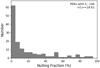 |
Fig. 9. Distribution of the average nulling fraction fn of 146 of the 214 known nulling pulsars. The averages are listed in Table C.1. |
4.2. Frequency dependence of nulling
For 22 pulsars for which nulling fractions are available for at least three frequency bands, their frequency dependencies are shown in Fig. 10. It is apparent that the nulling fractions are generally consistent across a wide rage of frequencies for PSRs J0814+7429, J0908−1739, J0953+0755, and J2018+2839, while for PSRs J0630−2834, J0820−1350, J1107−5907, J1709−1640, and J1946+1805, nulling fractions vary significantly across frequencies. For PSRs like J1136+1551 and J2048−1616, the estimated nulling fractions at high frequencies are smaller than the low-frequency ones. These diverse properties mean that the broad-band nulls are produced by physical processes with a global change of pulsar magnetosphere. During which, the distributions of relativistic particles may also have changed. The combined effects of the distributions of relativistic particles and pulsar geometry could lead to various nulling features.
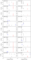 |
Fig. 10. Frequency dependencies of nulling fractions of 22 pulsars. Nulling fractions of these pulsars were estimated at least three frequencies. Red dots represent nulling fractions estimated at 2250 MHz from the present work, blue arrows are for the upper or lower limits. Values of nulling fractions and their references are listed in Table C.1. |
As emissions of different frequencies originate from different heights of pulsar magnetosphere (see, e.g., Wang et al. 2013). Relativistic particles emitting at different heights are generated from different polar cap regions through a sparking process. If nulls of a pulsar from simultaneous observations are frequency dependent, this means that parts of the polar cap region are inactive. In other words, frequency-dependent nulling can help us to distinguish the sparking polar cap regions. Any global change of pulsar magnetosphere will cause simultaneous nulling across a broad frequency band. PSR J1709−1640 has nulls lasting for minutes to hours, and observations over such limited time intervals can lead to different estimates of nulling fractions. Moreover, different modes might also cause different nulling fractions. For example, PSRs J0826+2637 and J1107−5907 have two modes with quite different nulling fractions (Young et al. 2014; Basu & Mitra 2019).
4.3. Dependence on pulsar parameters
Our observations of ten pulsars have multiple nulling cycles (Nc > 10), as listed in Table 2. Figure 11 shows correlations of nulling fraction, the cadence of occurrence of nulling Nc/Nsub, null-to-emission length ratios Nn/Ne, nulling degrees (α1 and α2), and nulling scales (s1 and s2) with respect to pulsar age and Edot for these pulsars. Here, nulling fractions and their uncertainties are taken as the mean and half range of upper and lower limits when both limits are available. Pulsars with large ages tend to have large nulling fractions with a correlation coefficient of 0.33, and to have small nulling scales with correlation coefficients of −0.30 and −0.35. Weak correlations are found for the other nulling parameters with respect to pulsar age. Pulsars with large energy loss rates tend to have small nulling fractions, small nulling cadence, and small null-to-emission length ratios with correlation coefficients of −0.69, −0.65, and −0.53, but tend to have large nulling scales with correlation coefficients of 0.49 and 0.61.
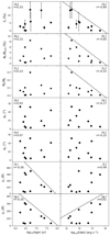 |
Fig. 11. Dependencies of nulling fraction, nulling cadence (Nc/Nsub), nulling to emission length ratios (Nn/Ne), nulling degrees (α1 and α2) and nulling scales (s1 and s2) on age and Edot for ten pulsars. Upper limits are plotted for fn, Nc/Nsub, Nn/Ne and s2 with respect to Edot, and for s1 and s2 with respect to age. Correlation coefficients are indicated in the corners of the panels. Values of fn, Nc, Nsub, Ne, Nn, α1, α2, s1 and s2 are listed in Table 2. |
Distribution of the nulling pulsars on the period and period derivative diagram is shown in Fig. 12. The periods of these nulling pulsars can be seen to range from 0.1 to 7 s and period derivatives to range from 10−18 to 10−12. The line with constant rate of loss of rotational kinetic energy (Edot) of 1030 erg s−1 roughly represents the lower boundary for these nulling pulsars, which is in parallel with the lines with constant accelerating potential above the pulsar polar cap. It is generally believed that pulsars are formed from the upper left part of the diagram and move down to the right by crossing the constant Edot lines when pulsars evolve. The particle acceleration process is reduced in the magnetosphere of aged pulsars, meaning that pulsars start to null with an increasing nulling fraction and eventually reach the off state. This scenario is supported by the distribution of pulsars with different nulling fractions in Fig. 12. It can be seen that pulsars with nulling fractions ≤1% are generally located in the upper left part of the diagram, and pulsars with nulling fractions > 30% are located in the lower right, as divided by the Edot line of 1032 erg s−1. The intermittent pulsars are exceptions (Lyne et al. 2017).
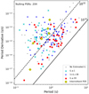 |
Fig. 12. Period derivative vs. period for 204 of the 214 known nulling pulsars for which a period and period derivative measurement are available. These pulsars are classified into five categories, that is, those without a nulling fraction estimation (small black dots), those with a nulling fraction of less than or equal to 1% (light blue “x”), those with a nulling fraction larger than 1% but less than 30% (blue “+”), those with a nulling fraction larger than or equal to 30% (large red dots), and intermittent pulsars. The two sloping lines are the constant rates of loss of rotational kinetic energy Edot = 1032, 1030 erg s−1. |
Figure 13 shows the correlations of nulling fraction with respect to pulsar period, period derivative, age, and Edot for this most complete sample of nulling pulsars to date. The nulling fraction is positively correlated with pulsar period with correlation coefficients of r = 0.26 and rl = 0.36 for both parameters in linear and logarithmic scales. No correlation is found for period derivatives. A marginal positive correlation is found between nulling fraction and pulsar age with r = 0.15 and rl = 0.12, which agrees with the understanding that old pulsars tend to have large nulling fractions. Moreover, the conventional understanding that pulsars with large Edot tend to have a small nulling fraction is also confirmed with correlation coefficients of r = −0.08 and rl = −0.30. In summary, large nulling fractions are more related to long periods than to large age and small Edot, which agrees with the conclusion obtained by Biggs (1992).
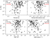 |
Fig. 13. Correlations of the nulling fraction with respect to pulsar period, period derivative, age, and Edot. Coefficients for linear and logarithmic correlations are indicated in each panel by r and rl. The nulling fraction of each pulsar is taken as the average as listed in Table C.1. Values of pulsar period, period derivative, age, and Edot are obtained from the ATNF pulsar catalog (Manchester et al. 2005). |
Acknowledgments
We thank the staff members of the Jiamusi deep space station and group members in NAOC for carrying out so many long observations. The authors are partially supported by the National Natural Science Foundation of China through grants (No. 11988101, No. 11873058), the Key Research Program of the Chinese Academy of Sciences (Grant No. QYZDJ-SSW-SLH021), and the Open Project Program of the Key Laboratory of FAST, NAOC, Chinese Academy of Sciences.
References
- Backer, D. C. 1970, Nature, 228, 42 [NASA ADS] [CrossRef] [Google Scholar]
- Basu, R., & Mitra, D. 2018, MNRAS, 476, 1345 [CrossRef] [Google Scholar]
- Basu, R., & Mitra, D. 2019, MNRAS, 487, 4536 [CrossRef] [Google Scholar]
- Basu, R., Mitra, D., & Melikidze, G. I. 2017, ApJ, 846, 109 [CrossRef] [Google Scholar]
- Basu, R., Mitra, D., & Melikidze, G. I. 2020, ApJ, 889, 133 [CrossRef] [Google Scholar]
- Bhat, N. D. R., Gupta, Y., Kramer, M., et al. 2007, A&A, 462, 257 [NASA ADS] [CrossRef] [EDP Sciences] [Google Scholar]
- Bhattacharyya, B., Gupta, Y., & Gil, J. 2010, MNRAS, 408, 407 [NASA ADS] [CrossRef] [Google Scholar]
- Biggs, J. D. 1992, ApJ, 394, 574 [NASA ADS] [CrossRef] [Google Scholar]
- Brinkman, C., Freire, P. C. C., Rankin, J., & Stovall, K. 2018, MNRAS, 474, 2012 [NASA ADS] [CrossRef] [Google Scholar]
- Burke-Spolaor, S., & Bailes, M. 2010, MNRAS, 402, 855 [NASA ADS] [CrossRef] [Google Scholar]
- Burke-Spolaor, S., Bailes, M., Johnston, S., et al. 2011, MNRAS, 416, 2465 [NASA ADS] [CrossRef] [Google Scholar]
- Burke-Spolaor, S., Johnston, S., Bailes, M., et al. 2012, MNRAS, 423, 1351 [NASA ADS] [CrossRef] [Google Scholar]
- Camilo, F., Ransom, S. M., Chatterjee, S., Johnston, S., & Demorest, P. 2012, ApJ, 746, 63 [NASA ADS] [CrossRef] [Google Scholar]
- Crawford, F., Altemose, D., Li, H., & Lorimer, D. R. 2013, ApJ, 762, 97 [CrossRef] [Google Scholar]
- Deich, W. T. S., Cordes, J. M., Hankins, T. H., & Rankin, J. M. 1986, ApJ, 300, 540 [NASA ADS] [CrossRef] [Google Scholar]
- Deneva, J. S., Stovall, K., McLaughlin, M. A., et al. 2016, ApJ, 821, 10 [NASA ADS] [CrossRef] [Google Scholar]
- Durdin, J. M., Large, M. I., Little, A. G., et al. 1979, MNRAS, 186, 39P [NASA ADS] [CrossRef] [Google Scholar]
- Faulkner, A. J., Stairs, I. H., Kramer, M., et al. 2004, MNRAS, 355, 147 [NASA ADS] [CrossRef] [Google Scholar]
- Filippenko, A. V., & Radhakrishnan, V. 1982, ApJ, 263, 828 [NASA ADS] [CrossRef] [Google Scholar]
- Force, M. M., & Rankin, J. M. 2010, MNRAS, 406, 237 [NASA ADS] [CrossRef] [Google Scholar]
- Gajjar, V., Joshi, B. C., & Kramer, M. 2012, MNRAS, 424, 1197 [NASA ADS] [CrossRef] [Google Scholar]
- Gajjar, V., Joshi, B. C., & Wright, G. 2014a, MNRAS, 439, 221 [NASA ADS] [CrossRef] [Google Scholar]
- Gajjar, V., Joshi, B. C., Kramer, M., Karuppusamy, R., & Smits, R. 2014b, ApJ, 797, 18 [NASA ADS] [CrossRef] [Google Scholar]
- Gajjar, V., Yuan, J. P., Yuen, R., et al. 2017, ApJ, 850, 173 [CrossRef] [Google Scholar]
- Han, J., Han, J. L., Peng, L.-X., et al. 2016, MNRAS, 456, 3413 [NASA ADS] [CrossRef] [Google Scholar]
- Herfindal, J. L., & Rankin, J. M. 2007, MNRAS, 380, 430 [NASA ADS] [CrossRef] [Google Scholar]
- Herfindal, J. L., & Rankin, J. M. 2009, MNRAS, 393, 1391 [NASA ADS] [CrossRef] [Google Scholar]
- Hotan, A. W., van Straten, W., & Manchester, R. N. 2004, PASA, 21, 302 [NASA ADS] [CrossRef] [Google Scholar]
- Huguenin, G. R., Taylor, J. H., & Troland, T. H. 1970, ApJ, 162, 727 [NASA ADS] [CrossRef] [Google Scholar]
- Ilie, C. D., Weltevrede, P., Johnston, S., & Chen, T. 2020, MNRAS, 491, 3385 [Google Scholar]
- Joshi, B. C., McLaughlin, M. A., Lyne, A. G., et al. 2009, MNRAS, 398, 943 [NASA ADS] [CrossRef] [Google Scholar]
- Kerr, M., Hobbs, G., Shannon, R. M., et al. 2014, MNRAS, 445, 320 [CrossRef] [Google Scholar]
- Kloumann, I. M., & Rankin, J. M. 2010, MNRAS, 408, 40 [CrossRef] [Google Scholar]
- Knispel, B., Eatough, R. P., Kim, H., et al. 2013, ApJ, 774, 93 [CrossRef] [Google Scholar]
- Kramer, M., Lyne, A. G., O’Brien, J. T., Jordan, C. A., & Lorimer, D. R. 2006, Science, 312, 549 [NASA ADS] [CrossRef] [PubMed] [Google Scholar]
- Lewandowski, W., Wolszczan, A., Feiler, G., Konacki, M., & Sołtysiński, T. 2004, ApJ, 600, 905 [NASA ADS] [CrossRef] [Google Scholar]
- Li, J., Esamdin, A., Manchester, R. N., Qian, M. F., & Niu, H. B. 2012, MNRAS, 425, 1294 [NASA ADS] [CrossRef] [Google Scholar]
- Lorimer, D. R., Camilo, F., & Xilouris, K. M. 2002, AJ, 123, 1750 [NASA ADS] [CrossRef] [Google Scholar]
- Lorimer, D. R., Lyne, A. G., McLaughlin, M. A., et al. 2012, ApJ, 758, 141 [NASA ADS] [CrossRef] [Google Scholar]
- Lynch, R. S., Boyles, J., Ransom, S. M., et al. 2013, ApJ, 763, 81 [NASA ADS] [CrossRef] [Google Scholar]
- Lyne, A. G., & Ashworth, M. 1983, MNRAS, 204, 519 [NASA ADS] [Google Scholar]
- Lyne, A. G., Stappers, B. W., Freire, P. C. C., et al. 2017, ApJ, 834, 72 [NASA ADS] [CrossRef] [Google Scholar]
- Manchester, R. N., Hobbs, G. B., Teoh, A., & Hobbs, M. 2005, AJ, 129, 1993 [NASA ADS] [CrossRef] [Google Scholar]
- Mitra, D., & Rankin, J. M. 2008, MNRAS, 385, 606 [CrossRef] [Google Scholar]
- Naidu, A., Joshi, B. C., Manoharan, P. K., & KrishnaKumar, M. A. 2017, A&A, 604, A45 [CrossRef] [EDP Sciences] [Google Scholar]
- Naidu, A., Joshi, B. C., Manoharan, P. K., & Krishnakumar, M. A. 2018, MNRAS, 475, 2375 [CrossRef] [Google Scholar]
- Rankin, J. M. 1986, ApJ, 301, 901 [NASA ADS] [CrossRef] [Google Scholar]
- Rankin, J. M., & Wright, G. A. E. 2007, MNRAS, 379, 507 [CrossRef] [Google Scholar]
- Rankin, J. M., & Wright, G. A. E. 2008, MNRAS, 385, 1923 [CrossRef] [Google Scholar]
- Rankin, J. M., Wright, G. A. E., & Brown, A. M. 2013, MNRAS, 433, 445 [NASA ADS] [CrossRef] [Google Scholar]
- Rankin, J. M., Olszanski, T. E. E., & Wright, G. A. E. 2020, ApJ, 890, 151 [CrossRef] [Google Scholar]
- Redman, S. L., & Rankin, J. M. 2009, MNRAS, 395, 1529 [NASA ADS] [CrossRef] [Google Scholar]
- Ritchings, R. T. 1976, MNRAS, 176, 249 [NASA ADS] [Google Scholar]
- Rosen, R., Swiggum, J., McLaughlin, M. A., et al. 2013, ApJ, 768, 85 [NASA ADS] [CrossRef] [Google Scholar]
- Smits, J. M., Mitra, D., & Kuijpers, J. 2005, A&A, 440, 683 [NASA ADS] [CrossRef] [EDP Sciences] [Google Scholar]
- Sobey, C., Young, N. J., Hessels, J. W. T., et al. 2015, MNRAS, 451, 2493 [NASA ADS] [CrossRef] [Google Scholar]
- Taylor, J. H., & Huguenin, G. R. 1971, ApJ, 167, 273 [NASA ADS] [CrossRef] [Google Scholar]
- van Straten, W., & Bailes, M. 2011, PASA, 28, 1 [NASA ADS] [CrossRef] [Google Scholar]
- Vivekanand, M. 1995, MNRAS, 274, 785 [NASA ADS] [Google Scholar]
- Wang, N., Manchester, R. N., & Johnston, S. 2007, MNRAS, 377, 1383 [NASA ADS] [CrossRef] [Google Scholar]
- Wang, P. F., Han, J. L., & Wang, C. 2013, ApJ, 768, 114 [CrossRef] [Google Scholar]
- Wang, P. F., Han, J. L., Han, L., et al. 2018, A&A, 618, A186 [CrossRef] [EDP Sciences] [Google Scholar]
- Weisberg, J. M., Armstrong, B. K., Backus, P. R., et al. 1986, AJ, 92, 621 [NASA ADS] [CrossRef] [Google Scholar]
- Weltevrede, P., Edwards, R. T., & Stappers, B. W. 2006, A&A, 445, 243 [NASA ADS] [CrossRef] [EDP Sciences] [Google Scholar]
- Weltevrede, P., Stappers, B. W., & Edwards, R. T. 2007, A&A, 469, 607 [NASA ADS] [CrossRef] [EDP Sciences] [Google Scholar]
- Wen, Z. G., Wang, N., Yuan, J. P., et al. 2016, A&A, 592, A127 [CrossRef] [EDP Sciences] [Google Scholar]
- Wright, G. A. E., & Fowler, L. A. 1981, A&A, 101, 356 [NASA ADS] [Google Scholar]
- Yan, W. M., Manchester, R. N., Wang, N., et al. 2020, MNRAS, 491, 4634 [CrossRef] [Google Scholar]
- Yang, A. Y., Han, J. L., & Wang, N. 2014, Sci. China Phys. Mech. Astron., 57, 1600 [CrossRef] [Google Scholar]
- Young, N. J., Weltevrede, P., Stappers, B. W., Lyne, A. G., & Kramer, M. 2014, MNRAS, 442, 2519 [CrossRef] [Google Scholar]
- Young, N. J., Weltevrede, P., Stappers, B. W., Lyne, A. G., & Kramer, M. 2015, MNRAS, 449, 1495 [CrossRef] [Google Scholar]
- Zhang, B., Qiao, G. J., & Han, J. L. 1997, ApJ, 491, 891 [NASA ADS] [CrossRef] [Google Scholar]
- Zhang, L., Li, D., Hobbs, G., et al. 2019, ApJ, 877, 55 [CrossRef] [Google Scholar]
Appendix A: Pulse sequences and null or emission states of 20 pulsars
We present plots here for observations of the 20 pulsars listed in Table 1. These plots show the pulse intensities of successive subintegrations formed every 2n pulses, the significance of on-pulse (red), and off-pulse (blue) emissions for each subintegration, and the emission (1) or null (0) state of the subintegration, as in Fig. 1. Here, n ranges from 0 to 5 depending on the significance of pulses.
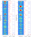 |
Fig. A.1. PSR J0034−0721 observed on 12 Dec 2015 (A and B) with every 32 pulses integrated. |
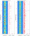 |
Fig. A.2. PSR J0248+6021 observed on 16 Jun 2015 and 11 Aug 2016 with every 32 pulses integrated. |
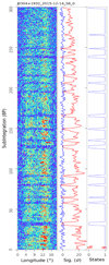 |
Fig. A.3. PSR J0304+1932 observed on 14 Dec 2015 with 8 pulse integrated for each subintegration. |
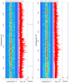 |
Fig. A.4. PSR J0332+5434 observed on 21 Feb 2016 (A and B) with single pulses. |
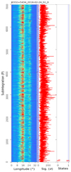 |
Fig. A.5. PSR J0332+5434 observed on 24 Feb 2016 with single pulses. |
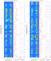 |
Fig. A.6. PSR J0528+2200 observed on 18 Jun 2015 and 17 Jan 2016 with subintegrations formed every 4 pulses. |
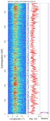 |
Fig. A.7. PSR J0543+2329 observed on 25 Jun 2015 with 16 pulses integrated for each subintegration. |
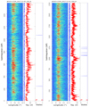 |
Fig. A.8. PSR J0543+2329 observed on 1 Nov 2017 (A and B) with 16 pulses integrated for each subintegration. |
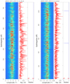 |
Fig. A.9. PSR J0826+2637 observed on 12 Nov 2015 (A and B) with every 4 pulses folded. |
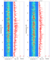 |
Fig. A.10. PSR J0826+2637 observed on 14 Nov 2015 (A and B) with every 4 pulses folded. |
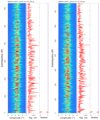 |
Fig. A.11. PSR J0826+2637 observed on 15 Nov 2015 (A and B) with every 4 pulses folded. |
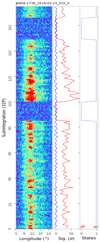 |
Fig. A.12. PSR J0908−1739 observed on 23 May 2016 and integrated every 32 pulses. |
 |
Fig. A.13. PSR J0922+0638 observed on 14 Jul 2015 and 17 Aug 2015 with subintegrations formed every 2 pulses. |
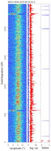 |
Fig. A.14. PSR J0922+0638 observed on 18 Aug 2015 with every 2 and pulses folded. |
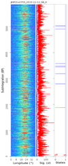 |
Fig. A.15. PSR J0953+0755 observed on 12 Dec 2015 with every 8 pulses folded. |
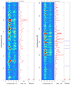 |
Fig. A.16. PSR J1136+1551 observed on 19 Sep 2015 and 16 Sep 2018 with 4 pulses folded for each subintegration. |
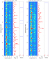 |
Fig. A.17. PSR J1136+1551 observed on 25 Oct 2017 (A and B) with 4 pulses folded for each subintegration. |
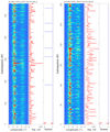 |
Fig. A.18. PSR J1136+1551 observed on 25 Oct 2017 (C and D) with 4 pulses folded for each subintegration. |
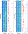 |
Fig. A.19. J1239+2453 observed on 12 Dec 2015 and 16 Dec 2015 with every 2 pulses folded. |
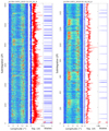 |
Fig. A.20. J1239+2453 observed on 19 Dec 2015 and 18 Feb 2016 with every 2 pulses folded. |
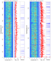 |
Fig. A.21. PSR J1509+5531 observed on 30 Oct 2017 (A and B) with single pulses. |
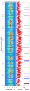 |
Fig. A.22. PSR J1709−1640 observed on 27 Oct 2017 with every 2 pulses folded. |
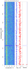 |
Fig. A.23. PSR J1844+00 observed on 9 Aug 2018 with 32 pulses folded for each subintegration. |
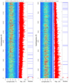 |
Fig. A.24. PSR J1932+1059 observed on 21 Feb 2016 (A and B) with single pulses. |
 |
Fig. A.25. PSR J1932+1059 observed on 21 Feb 2016 (C and D) with single pulses. |
 |
Fig. A.26. PSR J2022+5154 observed on 15 Jun 2015 and 1 Nov 2017 with single pulses. |
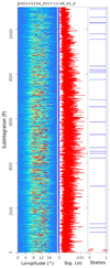 |
Fig. A.27. PSR J2022+5154 observed on 6 Nov 2017 with single pulses. |
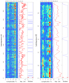 |
Fig. A.28. PSR J2048−1616 observed on 18 Jun 2015 and 8 Aug 2016 with every 2 pulses folded. |
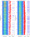 |
Fig. A.29. PSR J2313+4253 observed on 25 Oct 2017 (A and B) with single pulses. |
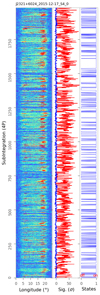 |
Fig. A.30. PSR J2321+6024 observed on 17 Dec 2015 with every 4 pulses folded. |
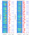 |
Fig. A.31. PSR J2321+6024 observed on 30 Oct 2017 (A and B) with every 4 pulses folded. |
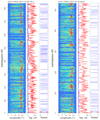 |
Fig. A.32. PSR J2321+6024 observed on 30 Oct 2017 (C and D) with every 4 pulses folded. |
Appendix B: Statistical analysis of nulling behaviors of the 20 pulsars
Statistical analysis on the nulling fractions are shown in Fig. B.1, emission and null lengths and their correlations in Fig. B.2, nulling periodicity in Fig. B.3, and intensity variations in Fig. B.4.
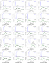 |
Fig. B.1. Histograms of the significance of on-pulses and off-pulses for the 20 pulsars. Normal functions with mean zero and standard derivation σoff are employed to model the distribution of off-pulse significance, scaled with fn and represented by a red dotted line. The residual distribution of on-pulse significance is plotted below and modeled by lognormal functions with mean μon and standard derivation σon. |
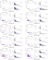 |
Fig. B.2. Emission and null lengths and their correlations for ten pulsars. Left panels: distributions of emission and null lengths. Length pairs for the emission and the following null are denoted as EN, and length pairs for the emission and its pre-null are denoted as NE. Correlation coefficients of emission lengths with respect to the null lengths are calculated and indicated in the top right corner for EN and NE. Histograms for the emission and null lengths are drawn in the top and right panels. Right panels: histograms of nulling degrees and scales of emission–null length pairs. The left hatched red step and right hatched blue step represent distributions for the EN and NE length pairs, respectively. The gray bars are for the simulated EN length pairs of randomly distributed emission–null sequence. |
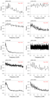 |
Fig. B.3. Average power spectrum for the ten pulsars, calculated from sliding Fourier transform of the emission–null (1–0) sequence in Appendix A. |
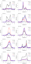 |
Fig. B.4. Integrated pulse profiles for ten pulsars. Profiles for the emission and nulls are represented by thick and thin black solid lines. For emission on states lasting for more than five pulses or subintegrations, profiles for the first and the second subintegration are represented by the thin and thick red dashed lines, and profiles for the last two subintegrations are represented by the thin and thick blue dash-dotted lines. |
Appendix C: Nulling pulsars reported hitherto
To date, 214 pulsars have been reported to null at various frequencies, including those collected from the literature and those presented in this work. These are classified into those with nulling fraction measurements, those without nulling fraction measurements, and intermittent pulsars. For each pulsar, the available nulling fractions are grouped into five frequency bands, 303−333, 408−430, 607−645, 1308−1518, and 2000−4850 MHz, as listed in Cols. (5)−(9). Column (10) presents the average nulling fractions, which are taken as half the upper limit if a pulsar has only an upper limit reported, or as 1.5 times the lower limit if a pulsar has only a lower limit.
Nulling fractions for 214 pulsars.
All Tables
All Figures
|
Fig. 1. Example of pulse sequence taken on 27 Oct 2017 for PSR J1709−1640. Left plots: part of the observation displayed with single pulses. Left panel: is for intensities of successive pulses. Right panel: is for the significance of on pulse (red) and off pulse (blue) emissions for each pulse. Middle plots: a much longer part of the observation taken for nulling analysis. The subintegrations are formed every two pulses, with its emission (1) or null (0) state indicated. Right plots: entire observation with subintegrations formed every 16 pulses. |
| In the text | |
|
Fig. 2. Histograms of the significance of on-pulses (gray hatched step) and off-pulses (blue no hatched step) for PSR J0908−1739 taken on 23 May 2016. The upper plots are for statistics of single pulses, and the lower plots are for subintegrations of every 32 pulses. The distribution of the off-pulse significance can be modeled with a normal function with a mean of zero and a standard deviation of σoff. The normal function is scaled with fn and represented by a red dotted line; it is subtracted from the distribution of on-pulse significance with the residuals indicated by black “plus” symbols in the panel. The residual distribution is modeled by a lognormal function with a mean of μon and a standard deviation of σon. Green solid, dash-dotted, and dashed lines are for the modeled distribution, the mean, and the lower three-sigma limit. |
| In the text | |
|
Fig. 3. Distributions of emission and null lengths of PSR J1709−1640. Pairs for the emission and the following null are denoted EN and are represented by red “o” symbol, while pairs for the emission and the pre-null are denoted NE and are represented by blue crosses. Nulling degrees, α1 and α2, and nulling scales, s1 and s2, are indicated for EN and NE. The correlation coefficients between emission and null lengths are shown in the top right corner. Histograms for the emission and null lengths are drawn in the top and right panels. Lengths of the longest emission or null state and their most probable and mean values are indicated in each panel. |
| In the text | |
|
Fig. 4. Histograms of nulling degrees and nulling scales of emission–null length pairs of PSR J1709−1640. The left hatched red step and right hatched blue step represent distributions for the EN and NE length pairs, respectively. The gray bars are for the EN length pairs of randomly distributed emission–null sequence from simulation. |
| In the text | |
|
Fig. 5. Sliding Fourier transform of the emission–null (1–0) sequence for PSR J1709−1640. The emission or null state of each subintegration is indicated in the left panel. Discrete Fourier transformation power from a box car of 1024 points is plotted in the main panel, which slides across the state sequence every 32 points. The average power is shown in the bottom panel. |
| In the text | |
|
Fig. 6. Tendency of pulse intensity variation during the emission states for PSRs J1709−1640 and J2313+4253, normalized by its average intensity and emission length. Black dots with error bars represent the average pulse intensity. |
| In the text | |
|
Fig. 7. Pulse profiles of PSRs J1709−1640 and J1509+5531 for the emission and nulls are represented by the thick solid and thin solid lines in black. Pulse profiles for the first and second subintegrations of the emission on states, E1 and E2, are represented by dashed lines in red, and those for the last and penultimate subintegrations, E−1 and E−2, are represented by dash-dotted lines in blue. |
| In the text | |
|
Fig. 8. Pulse sequences for the emission state setup (E1 − E4) and the transition to null (E−4 to E−1) for PSR J1509+5531. Null pulses are represented by the solid black lines. |
| In the text | |
|
Fig. 9. Distribution of the average nulling fraction fn of 146 of the 214 known nulling pulsars. The averages are listed in Table C.1. |
| In the text | |
|
Fig. 10. Frequency dependencies of nulling fractions of 22 pulsars. Nulling fractions of these pulsars were estimated at least three frequencies. Red dots represent nulling fractions estimated at 2250 MHz from the present work, blue arrows are for the upper or lower limits. Values of nulling fractions and their references are listed in Table C.1. |
| In the text | |
|
Fig. 11. Dependencies of nulling fraction, nulling cadence (Nc/Nsub), nulling to emission length ratios (Nn/Ne), nulling degrees (α1 and α2) and nulling scales (s1 and s2) on age and Edot for ten pulsars. Upper limits are plotted for fn, Nc/Nsub, Nn/Ne and s2 with respect to Edot, and for s1 and s2 with respect to age. Correlation coefficients are indicated in the corners of the panels. Values of fn, Nc, Nsub, Ne, Nn, α1, α2, s1 and s2 are listed in Table 2. |
| In the text | |
|
Fig. 12. Period derivative vs. period for 204 of the 214 known nulling pulsars for which a period and period derivative measurement are available. These pulsars are classified into five categories, that is, those without a nulling fraction estimation (small black dots), those with a nulling fraction of less than or equal to 1% (light blue “x”), those with a nulling fraction larger than 1% but less than 30% (blue “+”), those with a nulling fraction larger than or equal to 30% (large red dots), and intermittent pulsars. The two sloping lines are the constant rates of loss of rotational kinetic energy Edot = 1032, 1030 erg s−1. |
| In the text | |
|
Fig. 13. Correlations of the nulling fraction with respect to pulsar period, period derivative, age, and Edot. Coefficients for linear and logarithmic correlations are indicated in each panel by r and rl. The nulling fraction of each pulsar is taken as the average as listed in Table C.1. Values of pulsar period, period derivative, age, and Edot are obtained from the ATNF pulsar catalog (Manchester et al. 2005). |
| In the text | |
|
Fig. A.1. PSR J0034−0721 observed on 12 Dec 2015 (A and B) with every 32 pulses integrated. |
| In the text | |
|
Fig. A.2. PSR J0248+6021 observed on 16 Jun 2015 and 11 Aug 2016 with every 32 pulses integrated. |
| In the text | |
|
Fig. A.3. PSR J0304+1932 observed on 14 Dec 2015 with 8 pulse integrated for each subintegration. |
| In the text | |
|
Fig. A.4. PSR J0332+5434 observed on 21 Feb 2016 (A and B) with single pulses. |
| In the text | |
|
Fig. A.5. PSR J0332+5434 observed on 24 Feb 2016 with single pulses. |
| In the text | |
|
Fig. A.6. PSR J0528+2200 observed on 18 Jun 2015 and 17 Jan 2016 with subintegrations formed every 4 pulses. |
| In the text | |
|
Fig. A.7. PSR J0543+2329 observed on 25 Jun 2015 with 16 pulses integrated for each subintegration. |
| In the text | |
|
Fig. A.8. PSR J0543+2329 observed on 1 Nov 2017 (A and B) with 16 pulses integrated for each subintegration. |
| In the text | |
|
Fig. A.9. PSR J0826+2637 observed on 12 Nov 2015 (A and B) with every 4 pulses folded. |
| In the text | |
|
Fig. A.10. PSR J0826+2637 observed on 14 Nov 2015 (A and B) with every 4 pulses folded. |
| In the text | |
|
Fig. A.11. PSR J0826+2637 observed on 15 Nov 2015 (A and B) with every 4 pulses folded. |
| In the text | |
|
Fig. A.12. PSR J0908−1739 observed on 23 May 2016 and integrated every 32 pulses. |
| In the text | |
|
Fig. A.13. PSR J0922+0638 observed on 14 Jul 2015 and 17 Aug 2015 with subintegrations formed every 2 pulses. |
| In the text | |
|
Fig. A.14. PSR J0922+0638 observed on 18 Aug 2015 with every 2 and pulses folded. |
| In the text | |
|
Fig. A.15. PSR J0953+0755 observed on 12 Dec 2015 with every 8 pulses folded. |
| In the text | |
|
Fig. A.16. PSR J1136+1551 observed on 19 Sep 2015 and 16 Sep 2018 with 4 pulses folded for each subintegration. |
| In the text | |
|
Fig. A.17. PSR J1136+1551 observed on 25 Oct 2017 (A and B) with 4 pulses folded for each subintegration. |
| In the text | |
|
Fig. A.18. PSR J1136+1551 observed on 25 Oct 2017 (C and D) with 4 pulses folded for each subintegration. |
| In the text | |
|
Fig. A.19. J1239+2453 observed on 12 Dec 2015 and 16 Dec 2015 with every 2 pulses folded. |
| In the text | |
|
Fig. A.20. J1239+2453 observed on 19 Dec 2015 and 18 Feb 2016 with every 2 pulses folded. |
| In the text | |
|
Fig. A.21. PSR J1509+5531 observed on 30 Oct 2017 (A and B) with single pulses. |
| In the text | |
|
Fig. A.22. PSR J1709−1640 observed on 27 Oct 2017 with every 2 pulses folded. |
| In the text | |
|
Fig. A.23. PSR J1844+00 observed on 9 Aug 2018 with 32 pulses folded for each subintegration. |
| In the text | |
|
Fig. A.24. PSR J1932+1059 observed on 21 Feb 2016 (A and B) with single pulses. |
| In the text | |
|
Fig. A.25. PSR J1932+1059 observed on 21 Feb 2016 (C and D) with single pulses. |
| In the text | |
|
Fig. A.26. PSR J2022+5154 observed on 15 Jun 2015 and 1 Nov 2017 with single pulses. |
| In the text | |
|
Fig. A.27. PSR J2022+5154 observed on 6 Nov 2017 with single pulses. |
| In the text | |
|
Fig. A.28. PSR J2048−1616 observed on 18 Jun 2015 and 8 Aug 2016 with every 2 pulses folded. |
| In the text | |
|
Fig. A.29. PSR J2313+4253 observed on 25 Oct 2017 (A and B) with single pulses. |
| In the text | |
|
Fig. A.30. PSR J2321+6024 observed on 17 Dec 2015 with every 4 pulses folded. |
| In the text | |
|
Fig. A.31. PSR J2321+6024 observed on 30 Oct 2017 (A and B) with every 4 pulses folded. |
| In the text | |
|
Fig. A.32. PSR J2321+6024 observed on 30 Oct 2017 (C and D) with every 4 pulses folded. |
| In the text | |
|
Fig. B.1. Histograms of the significance of on-pulses and off-pulses for the 20 pulsars. Normal functions with mean zero and standard derivation σoff are employed to model the distribution of off-pulse significance, scaled with fn and represented by a red dotted line. The residual distribution of on-pulse significance is plotted below and modeled by lognormal functions with mean μon and standard derivation σon. |
| In the text | |
|
Fig. B.2. Emission and null lengths and their correlations for ten pulsars. Left panels: distributions of emission and null lengths. Length pairs for the emission and the following null are denoted as EN, and length pairs for the emission and its pre-null are denoted as NE. Correlation coefficients of emission lengths with respect to the null lengths are calculated and indicated in the top right corner for EN and NE. Histograms for the emission and null lengths are drawn in the top and right panels. Right panels: histograms of nulling degrees and scales of emission–null length pairs. The left hatched red step and right hatched blue step represent distributions for the EN and NE length pairs, respectively. The gray bars are for the simulated EN length pairs of randomly distributed emission–null sequence. |
| In the text | |
|
Fig. B.3. Average power spectrum for the ten pulsars, calculated from sliding Fourier transform of the emission–null (1–0) sequence in Appendix A. |
| In the text | |
|
Fig. B.4. Integrated pulse profiles for ten pulsars. Profiles for the emission and nulls are represented by thick and thin black solid lines. For emission on states lasting for more than five pulses or subintegrations, profiles for the first and the second subintegration are represented by the thin and thick red dashed lines, and profiles for the last two subintegrations are represented by the thin and thick blue dash-dotted lines. |
| In the text | |
Current usage metrics show cumulative count of Article Views (full-text article views including HTML views, PDF and ePub downloads, according to the available data) and Abstracts Views on Vision4Press platform.
Data correspond to usage on the plateform after 2015. The current usage metrics is available 48-96 hours after online publication and is updated daily on week days.
Initial download of the metrics may take a while.