| Issue |
A&A
Volume 697, May 2025
|
|
|---|---|---|
| Article Number | A198 | |
| Number of page(s) | 9 | |
| Section | Stellar structure and evolution | |
| DOI | https://doi.org/10.1051/0004-6361/202553813 | |
| Published online | 19 May 2025 | |
Simulation of the distribution of radio pulsar nulling fractions
1
Xinjiang Astronomical Observatory, Chinese Academy of Sciences, 150 Science 1-Street, Urumqi, Xinjiang 830011, China
2
Xinjiang Key laboratory of Radio Astrophysics, Chinese Academy of Sciences, 150 Science 1-Street, Urumqi, Xinjiang 830011, China
3
Key Laboratory of Radio Astronomy and Technology (Chinese Academy of Sciences), A20 Datun Road, Chaoyang District, Beijing 100101, PR China
4
SIfA, School of Physics, University of Sydney, Sydney, NSW 2006, Australia
⋆ Corresponding author: This email address is being protected from spambots. You need JavaScript enabled to view it.
Received:
20
January
2025
Accepted:
9
April
2025
Abstract
Aims. In this work, we aim to simulate the observed distribution of the pulse nulling fractions (NFs) in radio pulsars and to investigate the associated properties of the emission region.
Methods. We identified three conditions related to the occurrence of pulse nulling. From the traditional approach for correlation of the pulsed radio intensity and plasma density, a pulse cessation results from switching in the plasma density to zero. Second, recent observations have shown that the occurrence of a pulse cessation appears to favor certain emission conditions. Third, the observation of specific emission properties across different parts of a profile indicates that the emission region may be segmented. A detectable null would then correspond to the presence of a favorable condition, whereby the switching to zero plasma density occurs in all the emission segments visible to the observer. By dividing the emission region into equal segments around the magnetic axis, we simulated the distribution of NFs based on 5000 pulsar samples, each with 1000 rotations.
Results. Our results show that an emission region with 16 ± 4 segments gives the best-fit NF distribution for the recent observations. We find that while the number of nulling pulsars increases as their age increases, the NFs do not demonstrate a strong correlation with the obliquity angle, measured between the rotation and the magnetic axes. We show that the former relationship is related to the emission geometry, whereas the latter may be due to an additional mechanism on top of the traditional radio emission generation. The model predicts that nulling is expected to occur in all pulsars, although it is more common in pulsars of older ages.
Key words: stars: neutron / pulsars: general
© The Authors 2025
 Open Access article, published by EDP Sciences, under the terms of the Creative Commons Attribution License (https://creativecommons.org/licenses/by/4.0), which permits unrestricted use, distribution, and reproduction in any medium, provided the original work is properly cited.
This article is published in open access under the Subscribe to Open model. This email address is being protected from spambots. You need JavaScript enabled to view it. to support open access publication.
1. Introduction
One detectable feature found in more than 200 pulsars (Konar & Deka 2019; Wang et al. 2020) is manifested as a sudden cessation of the entire radio pulsed emission (Backer 1970; Rankin 1986; Wang et al. 2007; Young et al. 2015). Termed “pulse nulling”, the duration of the null pulses can vary significantly from several pulsar rotations to minutes (Konar & Deka 2019). Previous studies have shown that the occurrence of such emission cessation may be random in nature (Ritchings 1976; Biggs 1992; Wang et al. 2007). A useful quantification of the phenomenon is known as the nulling fraction (NF), which is a measure of the proportion of pulses without detectable emission in an observation (Gajjar et al. 2012). The NF is usually different for different pulsars (Wang et al. 2007; Gajjar et al. 2014a). This can be seen in the recent study by Wang et al. (2020), where they reported the distribution of the average NFs from 146 of the 214 known nulling pulsars. The data demonstrate a decrease in the number of pulsars as the NF increases, similarly to an exponential decay, which indicates certain underlying patterns for nulling. However, it is unclear how randomly occurring nulls could give rise to such an exponential distribution for the nulling fractions.
There are three pieces of information relevant to pulse cessation. The first is related to the intermittent pulsars. The emission of the pulsars changes quasi-periodically between radio “on” and “off” corresponding to pulses being detectable and undetectable (Kramer et al. 2006; Camilo et al. 2012; Lorimer et al. 2012; Lyne et al. 2017), respectively. This is similar to pulse nulling, but the nulls in the intermittent pulsars last for a much longer duration up to days and years. The phenomenon is interpreted as switching in the plasma density between two states of abundance and vacuum, with vacuum (zero plasma density) corresponding to the radio off (Kramer et al. 2006). The second information comes from the examination of pulse nulling. It shows that the occurrence of nulls may appear random, but the condition that is “favorable” for the phenomenon may be specific (Redman & Rankin 2009). This implies that certain conditions must be met for a pulsar to exhibit a null. The third piece of information comes from the observations of distinctive NF at different parts of an averaged profile in several pulsars. An example relates to PSR B2020+28, which displays different NFs between the leading and trailing components (Gajjar et al. 2012). Since observed emission features are linked to the emission properties (Ruderman & Sutherland 1975), these observations indicate that the emission properties are different at different parts of the profile (Rankin 1983). It also implies that different emission properties, correspond to different emission states, are allowed to co-exist in an emission region. We refer to an emission region (or open-field region) as locations where radio emission is generated and emitted (Ruderman & Sutherland 1975), similar to that depicted by Deshpande & Rankin (1999). By “emission state”, we refer to a specific value of the plasma charge density and a pulsar may jump suddenly between two or more different emission states (see Sect. 2.1). Furthermore, each of the emission states perform nulling differently, resulting in the NF being different over different parts of the emission region. However, it is unknown as to how the different emission states are arranged in an emission region. A possible arrangement can be inferred from the “partial” nulls in PSR J1819+1305, which shows that nulling can take place across only a smaller range of longitudinal phase within the pulse profile. It also indicates that changes in emission properties do not always occur concurrently across the whole radio emission region, but they are confined to segments in the region. From the rotating vector model (Radhakrishnan & Cooke 1969), emission observed at different parts of a profile may be considered to be coming from specific ranges of magnetic field line (Rankin 1983). The emission region may then be divided into segments, referred to as the emission segments (or just segments where there is no confusion), each of equal angular division and extending from the magnetic pole to the edge of an emission region. The emission segments fill up the emission region, and each possesses a particular emission state.
In this paper, we aim to simulate the distribution of nulling fractions as shown in the recent work by Wang et al. (2020). In Sect. 2, we adopt the same approach that we used previously for emission cessation (Han & Yuen 2022), based on switching in the plasma density to zero, and we extend it by introducing characteristics of the emission region and the restrictions for emission switching in relation to nulling. We assume that (i) pulse nulling is a manifestation of emission cessation across the whole profile; (ii) the cessation is due to switching in the plasma density to zero under favorable condition; and (iii) the emission region is divided into emission segments with the occurrence of point (ii) being separated in each segment. In Sect. 3, the procedures for our simulation are outlined and the resulting distribution is given in Sect. 4. Section 5 explores the implications of our results to the underlying mechanism. We discuss and present the conclusions to the paper in Sect. 6. The electromagnetic fields and the emission geometry are given in Appendices A and B, respectively, and the transformation matrices are given in Appendix C.
2. Modeling of pulse nulling
There is growing evidence to suggest that sudden changes in some pulsar magnetospheres can cause alterations in the observed radio emission features (e.g., Smits et al. 2005; Kramer et al. 2006; Lyne et al. 2017). These observations suggest that a pulsar magnetosphere can possess multiple emission states, each with distinct emission properties. A pulsar is also allowed to switch between different emission states, which then leads to changes in the observed emission features. In this section, we present the model for changes in the plasma charge density and its relation to emission cessation based on the model for pulsar magnetospheres of multiple emission states (Melrose & Yuen 2014). An essential feature of the model concerns the incorporation of obliquity, as opposed to an aligned rotator, and the inclusion of the inductive field (Cruz et al. 2021; Tolman et al. 2022).
2.1. Detectable changes in plasma charge density
We summarize the model for changes in the plasma charge density based on the works of Melrose & Yuen (2014) and Han & Yuen (2022). Most of the analysis in this section is derived from the two papers. The modeling of the pulsar radio emission process involves acceleration and pair production in gaps, and the associated screening of the electric field (Sturrock 1971; Ruderman & Sutherland 1975). For a pulsar magnetosphere that can exist in different emission states, the screening of the parallel electric field along the magnetic field lines implies a charge density, ρsn, given as (Melrose & Yuen 2014):
 (1)
(1)
where “sn” is short for synthesis of different emission states. Here, an emission state is denoted by the parameter y that takes a value between 0 and 1, with y = 0 representing the corotation charge density (Goldreich & Julian 1969) and y = 1 representing the minimal model (denoted by “min”) in which the charge density produces an electric field. The corotation charge density ρGJ is described by
 (2)
(2)
where Ecor is defined by Eq. (A.5). Setting y = 1 gives ρsn = ρmin, with
 (3)
(3)
where Eind∥ is the parallel component of the inductive electric field from an obliquely rotating magnetic dipole defined by Eq. (A.2), and b is the unit vector along the dipolar field lines. The minimal model in which the charge density produces an electric field gives a field of Emin, such that Emin = −Eind∥. In Eq. (1), a switch in the emission state is signified by a change in the y value, which leads to a change in ρsn.
The change is detectable provided that it occurs at locations visible to the observer and they can be specified in the geometry outlined in Appendix B. The geometry is defined by two angles, namely the viewing angle, ζ, between the rotation axis and the line of sight, and the obliquity angle, α, subtended from the rotation axis to the magnetic axis. Visible emission is then treated to originate from source points (or “visible points”) within the boundary of an open-field (emission) region and emit parallel to the line-of-sight direction and tangential to the dipolar field lines.
The polar angle for the visible point in the magnetic frame (subscript b), denoted by {θbV, ϕbV}, for a given rotational phase, ψ, can be determined using Eq. (B.1). The corresponding angles in the observer’s frame is signified by {θV, ϕV}. Figure 1 illustrates the geometry and the relative positions of the different angles. Figure 2 shows an example of the boundary for two emission regions at 0.2 rL using Eq. (B.4) by assuming that emission comes from the last closed field lines.
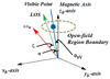 |
Fig. 1. Illustration of the pulsar viewing geometry in Cartesian coordinates using the angles of ζ = 25° and α = 35° in the magnetic frame. The magnetic axis is aligned with the zb-axis, and the line-of-sight (LOS) and the rotation axis are indicated by the green and red arrows, respectively. Also drawn is the boundary of an open-field region (dotted gray), centered at the magnetic pole. The orientation is chosen so that the magnetic axis, the rotation axis and the line-of-sight all lie in the xb − zb plane at ψ = 0°. At this phase, the visible point is located at {θbV, ϕbV}={6.7° , 0° }, as indicated by the blue dot. |
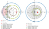 |
Fig. 2. Illustrations for two open-field (emission) regions at height 0.2 rL, bounded by dotted gray curve, are shown in the magnetic frame for α = 35° (left) and 10° (right). The size of the magnetosphere is assumed to be one unit. The rotation axis is stationary relative to the magnetic axis, with the location marked by the red triangle. Each emission region is divided into 20 equal emission segments around the magnetic pole that is located at the origin. Also illustrated, we have the null region in gray and the null area in pink (left-hand plot only). In the left-hand plot, three trajectories of the visible point are plotted using ζ = 65° (blue), 45° (green), and 25° (brown), while the location of the light-cylinder radius on the x-axis is indicated by a black vertical dotted line. In the right-hand plot, the two trajectories are obtained using ζ = 60° (blue), which does not cut the open-field region, and 20° (green). More details are given in the main text. |
Consider the left-hand plot, which contains three different trajectories of the visible point. Apart from an aligned rotator (α = 0°), the location of the visible point changes as the pulsar rotates. The visible point begins at ψ = 0° located on the x-axis closer to the origin when the magnetic and rotation axes and the line of sight are coplanar. Depending on the ζ and α, the visible point may or may not situate in the open-field region. Consider the blue trajectory, where the visible point is inside the open-field region, the location of the visible point changes with ψ tracing out a curve that traverses the open-field region, till the visible point exits at A2. The visible point continues to move intersecting the x-axis again when ψ = 180°, where the line of sight is on the far side of the magnetic axis. The visible point then completes the other half of the rotation entering the open-field region at A1 and, finally, back to ψ = 0°. From Eq. (B.1), it is apparent that trajectories of different ζ and α pairs are different, but the trajectories follow the similar pattern for every pulsar rotation. However, as shown in the left-hand and right-hand plots in Fig. 2, the trajectories will cut the open-field region differently or even miss it entirely, like the blue trajectory in the right-hand plot. A typical trajectory of the visible point is not circular and may (or may not) encompass the magnetic pole. Furthermore, the pulse window becomes a point (if only one pole is visible) at a particular ψ and from a minimum height, denoted by rmn with “mn” indicating minimum, where the trajectory is tangent to the boundary if emission comes only from the last closed field lines. This implies that the visible point is dependent on height, rV by Eq. (B.4), in the way that rV > rmn, for each open field line. The visible locations are situated at points designated by {rV, θV, ϕV} in the observer’s frame or in the magnetic frame as {rV, θbV, ϕbV} for given ζ and α. Since emission is assumed to occur only within the open-field region, only the part of a trajectory lying inside that region will the emission be detected. This leads to an increased intensity, forming a pulse profile, while being absent in other part of the trajectory, resulting in a “flat line” across those rotational phases. The similar condition applies to all the trajectories in Fig. 2. In this model, the pulse-width is the range of ψ on the trajectory that lies inside the emission region. For the blue trajectory in the left-hand plot, the range is between A1 and A2, while it is between B1 and B4 for the green trajectory, and between C1 and C2 for the brown trajectory. Assuming that the rotational phases at A1 and A2 on the blue trajectory are ψ1 and ψ2, respectively, would give the pulse-width as Δψ = ψ2 − ψ1. In the right-hand plot, the entire green trajectory lies inside the emission region, which means that emission is potentially detectable from the whole trajectory. The blue trajectory, being located outside of the open-field region, results in a flat line in the profile across the full rotational phase.
2.2. Emission cessation
From the traditional models, radio emission requires the production of secondary pairs characterized by a multiplicity, λ, that is greater than unity (Ruderman & Sutherland 1975; Beskin et al. 1993; Melrose & Yuen 2012). In this case, we would have λ = (n+ + n−)/nGJ ≫ 1 (Gurevich & Istomin 2007), where n± represents the number density of positrons and electrons and nGJ = ρGJ/e. In addition, radio radiation generated from highly relativistic plasma in two-stream instability suggests that the pulse intensity is proportional to the plasma density (Manchester & Taylor 1977; Cordes 1979; Lyubarskii 1996), given as ∝λρsn in our model. Assuming identical pair production in every emission state would imply that the pulse intensity is proportional to ρsn. Since our definition for the different allowed emission states is between y = 0 and y = 1 (inclusively), an emission cessation is considered legitimate, provided that the change in ρsn satisfies
![Mathematical equation: $$ \begin{aligned} \rho _{\rm sn}(y) = 0, y:=[0,1], \end{aligned} $$](/articles/aa/full_html/2025/05/aa53813-25/aa53813-25-eq4.gif) (4)
(4)
at a particular location in the emission region. All of the locations that satisfy Eq. (4) form the “null region”, illustrated in gray in Fig. 2. Only a subset of the whole emission region fulfills the switching described by Eq. (4), as illustrated in Fig. 2 by the gray shaded area. The dependence of the null region on α is also illustrated in the figure. As α decreases, the null region covers a large space in the emission region. This implies that trajectories of broader combinations of ζ and α will cut the null region (see Sect. 5). Hence, a detectable null corresponds to emission cessation satisfying Eq. (4) at every ψ across the range of the locations defined by Δψ along the trajectory of the visible point within the emission region.
The observation of partial nulls in PSR J1819+1305 (Rankin & Wright 2008) clearly suggests that pulse cessation can take place only in certain parts of the whole emission region. The emission of the pulsar appears to originate from two segments, between which only the one at later longitudinal phases goes to null. This implies that the emission region may be divided into segments each with its own properties of nulling. From the rotating vector model (Radhakrishnan & Cooke 1969), emission observed at different parts of a profile may be considered to be coming from specific magnetic field lines (Johnston & Weisberg 2006). In a dipolar structure, the equations for a field line are defined in the magnetic frame by r(θb) = r0sin2θb and Φ0 = ϕb, where r0 and Φ0 are the field line constant and the azimuthal position of the field line at the star’s surface, respectively. The arrangement of the open field lines is a function of the azimuthal angle about the magnetic axis and, hence, the boundary of the i-th segment may be defined by the angle subtended from ϕb1i to ϕb2i, with its size being proportional to Δϕbi = ϕb2i − ϕb1i (see Sect. 3). The two emission regions shown in Fig. 2 are each modeled with 20 segments, where Δϕbi = 18°, around the magnetic axis beginning from the negative x-axis. Emission switching represented by Eq. (4) can occur in the emission segments that overlap with the null region. For those segments that exhibit the switching, they together form the “null area” indicated in pink in the left-hand plot of Fig. 2. In the figure, switching occurs in consecutive segments giving one null area, However, switching segments can be separated and this will result in more than one null area in the emission region. Therefore, null areas are composed of different emission segments, where ρsn = 0. In addition, switching of ρsn = 0 takes place in a whole segment if the entire segment locates within the null region. There are emission segments that overlap only part of the null region, as shown by the segments on the right-hand side of the emission region in the right-hand plot in Fig. 2, where only their outer parts are in gray color. In this case, switching that satisfies Eq. (4) occurs only in the part of the segment that overlaps with the null region. Therefore, nulling is legitimate provided that the total range of ϕb, summed from consecutive segments with nulling, denoted by ΔϕbN, coincides with the part of the trajectory that lies inside the emission region, that is, ΔϕbN ≥ Δψ. In this way, the part of the normally emitting open region is said to undergo detectable null at the locations where the switching to ρsn = 0 occurs along the trajectory of the visible point that lies inside the open-field region.
An instance of null is shown in the left-hand plot in Fig. 2. The null area (pink) is consisted of six consecutive segments currently in null. The null area coincides with the blue trajectory inside the emission region indicating that the null is detectable. The similar emission cessation as seen by the green trajectory occurs only between B2 and B3 within the emission region and not the whole pulse from B1 to B4. According to our definition, the pulse cessation detected from the green trajectory does not count as a null. Part of the brown trajectory is located inside the emission region (between C1 and C2), but it is outside of the null area and the null region; this means that nulling is never detectable, thus making it a non-nulling pulsar from the perspective of the brown trajectory. Given that ϕb1i and ϕb2i are fixed but the condition for ρsn = 0 changes in each pulsar rotation, the frequency of nulling will also change as the pulsar rotates – and it may or may not be the same for different pulsars. The number occurrence of a null is defined by the number of times, n, that switching of ρsn = 0 occurs across the segments in the null region coinciding with the trajectory within the emission region. The nulling fraction is then given by the ratio of n to the total number of pulsar rotation, N, or NF = n/N.
2.3. Condition for pulse nulling
Studies show that the condition required for a null to occur may not be random and that it is perhaps related to certain emission features (Weltevrede et al. 2006; Redman & Rankin 2009). An example of the latter includes drifting subpulses, which exhibit as a systematic marching of subpulses across the pulse window (Manchester & Taylor 1977), and the occurrence of nulls appears to favor correlation with certain subpulse drift properties. This also implies that the exact condition favoring a pulse cessation is likely to be different for different pulsars. However, the exhibition of drifting subpulses or other emission features, such as giant pulses, in any pulsars is largely unpredictable. It follows that given a large sample of pulsars, the occurrence of the favorable condition for pulse nulling in a pulsar would appear random.
3. The simulation
We assume that the emission region can be divided into emission segments of equal size, with the number of segments being randomly selected between 1 and 45 for a sample pulsar. We also assume that each segment is capable of emission switching independent of each other. There are studies to show that the α values for radio pulsars tend to be small (Rookyard et al. 2015; Rankin 1990, 1993; Tauris & Manchester 1998). Here, we assign an α value to each pulsar sample, which is randomly generated from 1° ≤α ≤ 90° in steps of 0.5°. The sample is also given a ζ value, which is randomly selected from a range of 0° ≤ζ ≤ 90°, also in steps of 0.5°, with the restriction for the impact parameter |β|=|ζ − α|≤15° applied (Lyne & Manchester 1988; Wang et al. 2023a). A maximum emission height at 0.2 rL is also imposed (Johnston & Weisberg 2006). Next, the trajectory of the visible point and its part that lies within the emission region are determined. This gives ψ1 and ψ2, and hence Δψ. For a pair of {ζ, α} with 0 < Δψ ≤ 1, in steps of 0.1, the emission heights along the trajectory of the visible point between ψ1 and ψ2, in steps of 0.1°, are checked using Eq. (B.4) to ensure that they are all ≤0.2 rL. Then, the y values for ρsn = 0 for each ψ within Δψ are determined using Eq. (1) making sure that they satisfy Eq. (4). The above procedures are repeated until 5000 samples are obtained.
The next step in the simulation involves determining the nulling statistics for each sample pulsar. For particular values of {ζ, α}, nulling requires that the favorable condition for emission switching be present and that the actual switching of ρsn = 0 to occur in all the required segments cut by the trajectory of the visible point. Here, we assumed that the two processes are random and denote them as Q1 and Q2, respectively. The occurrence probability for each process is calculated based on an interval given by [0, sj], where sj is a value taken from the range between 0 and 1, in steps of 0.001, and j = 1 or 2 for Q1 or Q2, respectively. We can consider Q1 as an example. An interval is formed for each iteration in s1 resulting in 1001 different intervals. For each iteration in s1, another number denoted by n1 is generated randomly from the same range between 0 and 1. The condition for Q1 to occur requires fulfilling 0 ≤ n1 ≤ s1 for an iteration in s1. This is similar for Q2 for each of the emission segments cut by the trajectory of the visible point. The switching of ρsn = 0 will occur provided that 0 ≤ n2 ≤ s2. For a pulsar rotation, 0 ≤ n1 ≤ s1 for Q1 only needs to be met once, whereas 0 ≤ n2 ≤ s2 for Q2 needs to be satisfied for all the required segments. We further assumed that the default emission is radio-on in each pulsar rotation and the emission switching was determined separately for each segment in every rotation for 1000 pulsar rotations. A simulated distribution was then compared with the observed NF distribution obtained from the 146 known nulling pulsars, as presented by Wang et al. (2020). Two key features were identified from the observed distribution. When rounded to the nearest integer, they are (i) the peak occurs within the 5% NF followed by an immediate drop of about 70% and (ii) no NFs beyond about 90%. The two criteria were checked for each simulated distribution, while the matching distributions were visually examined to identify the best-fit candidate.
4. Distribution of the nulling fractions
The results of our simulation for the distribution of NFs from our samples are shown in Fig. 3. The normalized distribution is positively skewed towards higher NFs. It peaks at NF within 0.05 followed immediately by a drop of about 72% and then a gradual decrease until around NF = 0.2. After that, the number remains roughly constant before it begins to drop again at around NF = 0.6 and reaching zero beyond NF ≈ 0.9. The results are in close resemblance to our criteria. Since the pulse-width of normal pulsars ranges widely but likely to be about 0.1 in duty cycle, the trajectory of the visible point will likely cut more than one emission segment. In the simulation, the chance for having all the segments to null decreases as the number of segments increases. This leads to more samples with small NFs, but this number of samples gets smaller as the NF increases. We find that about 50% of the samples in our simulation possess NF of less than 0.07, consistent with the observations (Wang et al. 2020), and this increases to about 0.37 that covered by 80% of the samples. The average NF is 0.17. The normalized distribution for the length of the null pulses is shown in Fig. 4. It has a peak at around ten null pulses followed by an exponential decrease as the null length increases. The minimum and maximum null lengths are 1 and 641 pulses, respectively, with an average of 62.0 pulses in our sample.
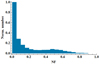 |
Fig. 3. Histogram showing the best-fit normalized distribution of the nulling fractions based on simulation of 5000 sample pulsars. |
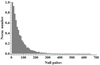 |
Fig. 4. Histogram showing the normalized distribution for the length of the null pulses. |
We find that an average of 16 ± 4 emission segments around the magnetic axis, combining with s1 = 0.03 and s2 = 0.5, give the best-fit distribution from our samples. Previous studies of drifting subpulses showed that the number of sub-beams may vary (Gil et al. 2003; Esamdin et al. 2005; Smits et al. 2005; Mitra & Rankin 2008) but it is roughly 20 (Deshpande & Rankin 1999; Gupta et al. 2004; Godoberidze et al. 2005; Bhattacharyya et al. 2009), which is consistent with our predicted number of emission segments. Our results show that while about 50% of the sample pulsars achieve ρsn = 0 for y ≈ 1, which is near vacuum in the magnetosphere, there are pulsars that give ρsn = 0 with lower y values. However, no nulls were detected with y = 0. This implies that pulse nulling (ρsn = 0) cannot occur in a corotating magnetosphere (y = 0).
Some studies suggest the existence of a “break” at approximately 40% in the NF distribution (Konar & Deka 2019). Subsequent investigations showed that such a “break” is statistically insignificant (Sheikh & MacDonald 2021). To optimally fit the observations, our distribution of NFs is continuous until it reaches zero at around NF = 0.9. However, we find that a local minimum would appear, becoming more prominent, and eventually forms a break in the distribution, as s1 in Q1 increases suggesting its relation to the necessary condition for switching in our model. In our simulation, decreasing the number of samples has impact on the distribution, which implies that a larger sample size may improve the observational results (Sheikh & MacDonald 2021).
5. Implications of the underlying mechanism
In the simulation, nulls are found in pulsars with different α values. Specifically, the number of nulling pulsars increases as α decreases, which suggests that nulling is more common in pulsars with small α. On the contrary, the NFs do not show a significant correlation with α, although slightly more pulsars with α ≲ 20° possess smaller NFs. From the consideration of energy loss through magnetic dipole radiation, pulsar braking decreases as α reduces (Manchester & Taylor 1977; Lyubarskii & Kirk 2001), which means that α changes from large to small. For pulsar braking owing to the longitudinal current flow and the production of secondary particles (Beskin et al. 1988), the plasma density decreases with increasing α (Goldreich & Julian 1969), implying that α evolves from small to large. In addition, radio emission is suggested in relation to an accelerating potential and the latter decreases as the rotation period increases leading to a pulsar’s death (Arons 2000; Zhang et al. 2000; Harding & Muslimov 2002). In both evolutionary models, the pulsar’s age and rotation period are related to α. The fact that more nulling pulsars are found at small α implies that the variation of the former is a function of the pulsar’s age and rotation period (Ritchings 1976; Biggs 1992). This also suggests that nulling is connected to the emission geometry. In our model (described in Sect. 2.2), the range of θ covered by a null region around ψ = 0 (the fiducial point) becomes narrower as α increases, while the restriction on β remains unchanged. Hence, the corresponding average emission height would be higher when we are assuming that the emission only comes from the last closed field lines. This, in turn, is not favorable to the assumption that radio emission comes from low emission heights. As for the NFs, the lack of a significant correlation with α implies that the former is not likely related to pulsar’s age (Rankin 1986). A trajectory of the visible point cutting a null region signifies that it is a nulling pulsar. The occurrence of a null also requires switching to take place in Q1 and Q2 irrespective of α. Both are assumed to be random in our model and, hence, the resulting NFs would also appear non-correlative with α. It implies that the frequency of null may be governed by a different mechanism in addition to the traditional radio generation, which is dependent on α.
Our assumption that an emission region is composed of multiple emission segments of equal size suggests the dependency of the emission properties on the longitudinal phase. It implies that the change in emission could be unique at different parts of the emission region. This is seen in other emission features, including drifting subpulses of different drift-rates across different parts of the same pulse window (Weltevrede et al. 2006; Weltevrede 2016; Gajjar et al. 2017; Szary & van Leeuwen 2017), and profile mode-changing, where distinct shape changes are observed at different parts of an averaged profile. In addition, our results show that the amount of detectable emission segments is dependent on the pulse-width. As shown in Fig. 2, a broader profile results from the trajectory of the visible point cutting a larger part of an emission region, which, in turn, contains multiple emission segments. Increasing number of segments means that a consistent emission feature would require similar emission properties across more adjacent segments. This would also imply that NF is likely be large in pulsars with narrow pulse-width because the trajectory now traversing a smaller part of the emission region and hence cutting lesser emission segments. The probability for all the required emission segments to switch to null changes with different pulse-widths. This is consistent with some observations that showed correlation between NF and pulse-width (Biggs 1992; Li & Wang 1995; Sheikh & MacDonald 2021). In general, radio profiles have duty cycles of less than 0.1 – or about two emission segments if a total of 20 segments is assumed. Therefore, it is more likely for a pulsar to have consistent emission features across the observable profile.
6. Discussion and conclusions
We performed simulations of the distribution of nulling fractions based on the assumption that nulling is a manifestation of pulse cessation due to a switching of the plasma density to zero. The occurrence of such switching is assumed to also rely on the presence of a favorable condition and both are thought to take place randomly. The detectability of pulse nulling is based on a purely geometric model defined by ζ and α, where the visible emission locations are specified by the locus along the trajectory of the visible point that cuts the emission region of a pre-defined maximum height. We assume that a pulsar emission region is composed of multiple emission segments, each of which can cause switching in the plasma charge density between zero and non-zero, with zero charge density signifying cessation in the emission. A sample in our simulation is said to exhibit a null when the favorable condition is met and switching occurs in all the segments that are traversed by the trajectory of the visible point. Our results indicate that the meeting of the favorable condition for switching is a lower probability event than that of switching to zero plasma density. We found that 16 ± 4 emission segments lead to a distribution of nulling fractions that offers the best fit to that obtained from the pulsar data.
Overall, there are two proposals for nulling. One proposal relates the phenomenon to emission geometry, such that nulling is the result of the line of sight no longer cutting the emission beams (Timokhin 2010). The suggested change is in the re-arrangement of the open field lines, causing the emission beams to become re-oriented (Filippenko & Radhakrishnan 1982). Pulse nulling occurs if the changes take place across the azimuthal angles (around the magnetic axis) that coincide with or larger than the part of the emission region detectable to the observer. However, more observations display accompanying changes in emission properties around nulls, which indicate that the cause of nulling is more than merely a geometric origin. For example, the exhibition of emission on and off in the intermittent pulsars is also seen to correlate with a change in the spin-down ratio (Kramer et al. 2006). This implies a causal link between the radio emission and the global current that transmits the torque on the star. Timokhin (2010) suggests that the polar cap can change affecting both the current (and hence the torque) and the field lines on which the emission occurs, thus causing variation in the visibility of the emission. The other proposal refers the phenomenon to the temporary loss of the coherent radio emission in relation to the plasma production in the polar gap (Deich et al. 1986; Daugherty & Harding 1986). There are also models that combine emission geometry (Timokhin 2010; Dyks 2021). In our model, nulling is due to switching in the emission state leading to a drop in the plasma density to zero in some or all of the emission segments in the emission region. Each of the emission segments occupies an equal range of ϕb around the magnetic axis. The emission segments that achieve ρsn = 0 will go to null, while others will continue to be emitting. This forms an emission-null pattern in the whole emission region. Since emission switching occurs in every pulsar rotation, any emission or null in each segment will change from pulse to pulse. Therefore, the corresponding emission-null pattern is constantly changing. Furthermore, since the trajectory of the visible point does not change for a combination of ζ and α, but the locations for null (or emission) change, the emission-null pattern will also change over the part of the trajectory that lies inside the emission region. An emitting segment will suddenly turn into null when switching occurs. From the observer’s perspective, this would appear as if the line of sight misses the emission beam. In addition, the emission switching as signified by a change in the plasma charge density is linked to the pair production (as discussed in Sect. 2.2). This is in agreement with the proposal for nulling being attributed to a momentary loss in the coherent radio emission (with ρsn switching between nonzero and zero) in relation to the plasma production. Thus, our modeling of pulse nulling combines ingredients from both the geometric origin and plasma production.
Single-pulse studies in some pulsars have shown that pulse nulling is correlated with the observing frequency (Taylor et al. 1975; Bartel & Sieber 1978; Bhat et al. 2007; Gajjar et al. 2014b). The assumption of radio emission from dipolar magnetic field lines leads to the suggestion of the radius-to-frequency mapping (RFM; Cordes 1978). It states that emissions at different frequencies may be associated with emitting sources locating at distinct heights. It follows that radiation at lower frequency comes from a greater height and vice versa. The emission geometry described in Appendix B implies that visible emission at a given frequency comes from only one height at r = rV. Hence, the emission height will be higher for emission that originates at a lower frequency. From Fig. 2, a larger r corresponds to the locus of a trajectory occupying larger values of xb and yb. Since an emission segment extends from the magnetic pole to the boundary of an open-field region located at certain height, the trajectory may still traverse the null area but at different locations. Furthermore, our model assumes that detectable nulls are due to changes in ρsn through switching in y and they should occur in the whole emission segment and simultaneously across all the required emission segments. This implies a correlation of the phenomenon with different frequencies. However, it is also possible that emission switching at different parts of a segment is not identical, which leads to the observed nulling being not correlated across different frequencies. The description for such asynchronous emission switching requires a generalization to allow y to be a function of height along a specific field line. A possible approach relates to the parallel electric field (E∥) not being zero everywhere in a pulsar magnetosphere, which gives rise to a region where E∥ ≠ 0; this is known as the vacuum gap, where the field lines are not equipotential. One implication, as interpreted in the Ruderman & Sutherland (1975) model, is the variation in the plasma flow that is different below and above the gap, with the former being closer to corotation (y ≈ 0). It follows that the value of y is different across the gap, thereby implying different switching at different heights. This may be the case for some pulsars and, thus, nulling correlated at different frequencies would require the emission switching to be coordinated among all the different emission states.
Our requirement for emission cessation across the whole pulse during nulling is not manifested in every trajectory of the visible point. For example, in the left-hand plot in Fig. 2, the green trajectory intersects the null region, which consists of 12 segments – but only 6 of them exhibit switching. In that particular case, the two parts of the trajectory near the entry and exit of the emission region are still emitting, thereby making the pulse a “partial” nulling. When the favorable condition is met again, switching occurs in different emission segments causing the locations of the null areas to change. This results in variations in the pulse shape and intensity, including the occurrence of a null. Since switching is assumed to occur in every segment, variations in the pulse will also be seen in the blue trajectory. The pulse would appear as sometimes emitting and sometimes a null, with occasional partial nulling.
Another scenario occurs with trajectories that cut through the emission region, but where only part of the trajectory lies in the null region. In this case, emission from the part that lies in the emission region (but not in the null region) will always continue to emit. However, the other part, which lies in the null region, may sometimes go to null. The pulse will appear as always emitting with occasional “partial” nulls. Since trajectories of different ζ and α values will cut the null region differently, the number of intersecting emission segments will also change. In the case when only a small number of segments is cut, the pulses may appear to simply be alternating between emission and nulling. There is another similar emission change, which demonstrates as sudden transition in the shape of the averaged pulse profile between different quasi-stable modes (Backer 1970; Wang et al. 2007; Chen et al. 2011). Coined as profile mode-changing, it defies the rule that summing a sufficient number (usually ≳ 500) of single pulses would yield a stable averaged profile (Manchester & Taylor 1977). While nulling is a single-pulse event for most pulsars, the occurrence of profile mode-changing is usually at longer timescales (Lyne 1971; Wang et al. 2007; Wen et al. 2020). In our model, if we consider merely the change in the profile shape between different profile modes, it would imply that the occurrences of Q1 and Q2 are at longer time intervals. Furthermore, this time interval would be different for different pulsars. It follows that while pulse nulling and profile mode-changing might share many similarities, there are also differences that would suggest there are distinct processes underlying the two phenomena.
Traditional models make no distinction between nulling and ordinary (non-nulling) pulsars. Our model for emission switching in relation to changes in the plasma charge density predicts that nulling can occur in pulsars with different α. If we ignore the emission geometry and assume the favorable condition is always present, this implies that the two types of pulsars differ only in terms of the switch rate. It also means that nulling pulsars would correspond to switching to an emission state of ρsn = 0 occurring frequently enough to have been observed. In our simulation, the maximum NF is more than five times greater than the average value. This may give the illusion that pulse nulling in some pulsars is relatively easier to detect. However, the recent discoveries of nulling pulsars by the Five-hundred-meter Aperture Spherical Telescope (FAST; Li et al. 2018) suggests otherwise. One example relates to the pulsar PSR J1900+4221 (Tedila et al. 2022), which possesses an NF of about 0.2, but with a relatively low estimated flux density of about 2 mJy at the peak of the averaged profile. It may be the case that some nulling pulsars show low flux density and high NFs, making them difficult to discover. This has impact to pulsar searching, as large NF in pulsars with low flux density will make the search challenging if the observing time per target is too short. Even pulsars with small NF would still require long observing times to collect a significant amount of null pulses. However, both in observations (Wang et al. 2020) and in our prediction (see Fig. 3), we see a higher number of nulling pulsars with low NFs. With the construction of the large and highly sensitive telescopes, such as the QiTai radio Telescope (QTT; Wang 2014; Wang et al. 2023b), and telescope arrays, including the Square Kilometer Array (SKA), there is no doubt that more nulling pulsars will be discovered. This will improve the sample, enabling future investigations of nulling properties to provide important additional details that will help resolve the mechanism that underlies pulse nulling.
Acknowledgments
We thank the XAO pulsar group for useful discussions. We also thank the referee for useful comments, which helped improve the presentation of the paper. We thank the second referee for comments. R.Y. is supported by the National Key Program for Science and Technology Research and Development No. 2022YFC2205201, the National SKA Program of China No. 2020SKA0120200, the National Natural Science Foundation of China (NSFC) project (No. 12041303, 12041304, 12288102), the Major Science and Technology Program of Xinjiang Uygur Autonomous Region No. 2022A03013-2, 2022A03013-4. This research is partly supported by the Operation, Maintenance and Upgrading Fund for Astronomical Telescopes and Facility Instruments, budgeted from the Ministry of Finance of China (MOF) and administrated by the CAS.
References
- Arons, J. 2000, in Pulsar Astronomy – 2000 and Beyond, eds. M. Kramer, N. Wex, & R. Wielebinski (San Francisco: Astronomical Society of the Pacific), Proc. IAU Colloq., 177, 449 [Google Scholar]
- Backer, D. C. 1970, Nature, 228, 42 [NASA ADS] [CrossRef] [Google Scholar]
- Bartel, N., & Sieber, W. 1978, A&A, 70, 307 [NASA ADS] [Google Scholar]
- Beskin, V., Gurevich, A. V., & Istomin, Y. N. 1988, Ap&SS, 146, 205 [NASA ADS] [CrossRef] [Google Scholar]
- Beskin, V., Gurevich, A. V., & Istomin, Y. N. 1993, Physics of the Pulsar Magnetosphere (CUP) [Google Scholar]
- Bhat, N. D. R., Gupta, Y., Kramer, M., et al. 2007, A&A, 462, 257 [NASA ADS] [CrossRef] [EDP Sciences] [Google Scholar]
- Bhattacharyya, B., Gupta, Y., & Gil, J. 2009, MNRAS, 398, 1435 [NASA ADS] [CrossRef] [Google Scholar]
- Biggs, J. D. 1992, ApJ, 394, 574 [NASA ADS] [CrossRef] [Google Scholar]
- Camilo, F., Ransom, S. M., Chatterjee, S., Johnston, S., & Demorest, P. 2012, ApJ, 746, 63 [Google Scholar]
- Chen, J. L., Wang, H. G., Wang, N., et al. 2011, ApJ, 741, 48 [Google Scholar]
- Cordes, J. M. 1978, ApJ, 222, 1006 [NASA ADS] [CrossRef] [Google Scholar]
- Cordes, J. M. 1979, Space Sci. Rev., 24, 567 [NASA ADS] [CrossRef] [Google Scholar]
- Cruz, F., Grismayer, T., & Silva, L. 2021, Phys. Rev. E, 103, L051201 [Google Scholar]
- Daugherty, J. K., & Harding, A. K. 1986, ApJ, 309, 362 [NASA ADS] [CrossRef] [Google Scholar]
- Deich, W. T. S., Cordes, J. M., Hankins, T. H., & Rankin, J. M. 1986, ApJ, 300, 540 [Google Scholar]
- Deshpande, A. A., & Rankin, J. M. 1999, ApJ, 524, 1008 [NASA ADS] [CrossRef] [Google Scholar]
- Dyks, J. 2021, A&A, 653, L3 [NASA ADS] [CrossRef] [EDP Sciences] [Google Scholar]
- Esamdin, A., Lyne, A. G., Graham-Smith, F., et al. 2005, MNRAS, 356, 59 [NASA ADS] [CrossRef] [Google Scholar]
- Filippenko, A. V., & Radhakrishnan, V. 1982, ApJ, 263, 828 [Google Scholar]
- Gajjar, V., Joshi, B. C., & Kramer, M. 2012, MNRAS, 424, 1197 [Google Scholar]
- Gajjar, V., Joshi, B. C., & Wright, G. 2014a, MNRAS, 439, 221 [CrossRef] [Google Scholar]
- Gajjar, V., Joshi, B. C., Kramer, M., Smith, R., & Karuppusamy, R. 2014b, ApJ, 797, 18 [Google Scholar]
- Gajjar, V., Yuan, J. P., Yuen, R., et al. 2017, ApJ, 850, 173 [NASA ADS] [CrossRef] [Google Scholar]
- Gangadhara, R. T. 2004, ApJ, 609, 335 [NASA ADS] [CrossRef] [Google Scholar]
- Gil, J. A., Melikidze, G. I., & Geppert, U. 2003, A&A, 407, 315 [NASA ADS] [CrossRef] [EDP Sciences] [Google Scholar]
- Godoberidze, G., Machabeli, G. Z., Melrose, D. B., & Luo, Q. 2005, MNRAS, 360, 669 [NASA ADS] [CrossRef] [Google Scholar]
- Goldreich, P., & Julian, W. H. 1969, ApJ, 157, 869 [Google Scholar]
- Gupta, Y., Gil, J., Kijak, J., & Sendyk, M. 2004, A&A, 426, 229 [NASA ADS] [CrossRef] [EDP Sciences] [Google Scholar]
- Gurevich, A. V., & Istomin, Y. N. 2007, MNRAS, 377, 1663 [NASA ADS] [CrossRef] [Google Scholar]
- Han, X. H., & Yuen, R. 2022, ApJ, 940, 110 [Google Scholar]
- Harding, A. K., & Muslimov, A. G. 2002, ApJ, 568, 862 [NASA ADS] [CrossRef] [Google Scholar]
- Hones, E. W., Jr., & Bergeson, J. E. 1965, J. Geophys. Res., 70, 4951 [NASA ADS] [CrossRef] [Google Scholar]
- Johnston, S., & Weisberg, J. M. 2006, MNRAS, 368, 1856 [NASA ADS] [CrossRef] [Google Scholar]
- Konar, S., & Deka, U. 2019, JApA, 40, 42 [Google Scholar]
- Kramer, M., Lyne, A. G., O’Brien, J. T., Jordan, C. A., & Lorimer, D. R. 2006, Science, 312, 549 [NASA ADS] [CrossRef] [Google Scholar]
- Li, X. D., & Wang, Z. R. 1995, ChA&A, 19, 302 [Google Scholar]
- Li, D., Wang, P., Qian, L., et al. 2018, IEEE Microw. Mag., 19, 112 [CrossRef] [Google Scholar]
- Lorimer, D. R., Lyne, A. G., McLaughlin, M. A., et al. 2012, ApJ, 758, 141 [NASA ADS] [CrossRef] [Google Scholar]
- Lyne, A. G. 1971, MNRAS, 153, 27P [Google Scholar]
- Lyne, A. G., & Manchester, R. N. 1988, MNRAS, 234, 477 [NASA ADS] [CrossRef] [Google Scholar]
- Lyne, A. G., Stappers, B. W., Freire, P. C. C., et al. 2017, ApJ, 834, 72 [NASA ADS] [CrossRef] [Google Scholar]
- Lyubarskii, Y. E. 1996, A&A, 308, 809 [NASA ADS] [Google Scholar]
- Lyubarskii, Y. E., & Kirk, J. G. 2001, ApJ, 547, 437 [NASA ADS] [CrossRef] [Google Scholar]
- Manchester, R. N., & Taylor, J. H. 1977, Pulsars (San Francisco: W. H. Freeman) [Google Scholar]
- Melrose, D. B. 1967, Planet. Space. Sci., 15, 381 [NASA ADS] [CrossRef] [Google Scholar]
- Melrose, D. B., & Yuen, R. 2012, ApJ, 745, 169 [NASA ADS] [CrossRef] [Google Scholar]
- Melrose, D. B., & Yuen, R. 2014, MNRAS, 437, 262 [NASA ADS] [CrossRef] [Google Scholar]
- Mitra, D., & Rankin, J. M. 2008, MNRAS, 385, 606 [NASA ADS] [CrossRef] [Google Scholar]
- Radhakrishnan, V., & Cooke, D. J. 1969, Astrophys. Lett., 3, 225 [NASA ADS] [Google Scholar]
- Rankin, J. M. 1983, ApJ, 274, 333 [NASA ADS] [CrossRef] [Google Scholar]
- Rankin, J. M. 1986, ApJ, 301, 901 [Google Scholar]
- Rankin, J. M. 1990, ApJ, 352, 247 [Google Scholar]
- Rankin, J. M. 1993, ApJS, 85, 145 [NASA ADS] [CrossRef] [Google Scholar]
- Rankin, J. M., & Wright, G. A. E. 2008, MNRAS, 385, 1923 [NASA ADS] [CrossRef] [Google Scholar]
- Redman, S. L., & Rankin, J. M. 2009, MNRAS, 395, 1529 [NASA ADS] [CrossRef] [Google Scholar]
- Ritchings, R. T. 1976, MNRAS, 176, 249 [NASA ADS] [Google Scholar]
- Rookyard, S. C., Weltevrede, P., & Johnston, S. 2015, MNRAS, 446, 3367 [NASA ADS] [CrossRef] [Google Scholar]
- Ruderman, M., & Sutherland, P. G. 1975, ApJ, 196, 51 [NASA ADS] [CrossRef] [Google Scholar]
- Sheikh, S. Z., & MacDonald, M. G. 2021, MNRAS, 502, 4669 [Google Scholar]
- Smits, J. M., Mitra, D., & Kuijpers, J. 2005, A&A, 440, 683 [NASA ADS] [CrossRef] [EDP Sciences] [Google Scholar]
- Sturrock, P. 1971, ApJ, 164, 529 [Google Scholar]
- Szary, A., & van Leeuwen, J. 2017, ApJ, 845, 95 [NASA ADS] [CrossRef] [Google Scholar]
- Tauris, T. M., & Manchester, R. N. 1998, MNRAS, 298, 625 [NASA ADS] [CrossRef] [Google Scholar]
- Taylor, J. H., Manchester, R. N., & Huguenin, G. R. 1975, ApJ, 195, 513 [NASA ADS] [CrossRef] [Google Scholar]
- Tedila, H. M., Yuen, R., Wang, N., et al. 2022, ApJ, 929, 171 [Google Scholar]
- Timokhin, A. N. 2010, MNRAS, 408, L41 [NASA ADS] [CrossRef] [Google Scholar]
- Tolman, E. A., Philippov, A. A., & Timokhin, A. N. 2022, ApJ, 933, L37 [CrossRef] [Google Scholar]
- Wang, N. 2014, Sci. Sin. Phys. Mech. Astron., 44, 783, (Chinese version) [Google Scholar]
- Wang, N., Manchester, R. N., & Johnston, S. 2007, MNRAS, 377, 1383 [Google Scholar]
- Wang, P. F., Han, J. L., Han, L., et al. 2020, A&A, 644, A73 [NASA ADS] [CrossRef] [EDP Sciences] [Google Scholar]
- Wang, P. F., Han, J. L., Xu, J., et al. 2023a, Res. Astron. Astrophys., 23, A02 [Google Scholar]
- Wang, N., Xu, Q., Ma, J., et al. 2023b, Sci. China Phys. Mech. Astron., 66, 289512 [Google Scholar]
- Weltevrede, P. 2016, A&A, 590, A109 [NASA ADS] [CrossRef] [EDP Sciences] [Google Scholar]
- Weltevrede, P., Edwards, R. T., & Stappers, B. 2006, A&A, 445, 243 [NASA ADS] [CrossRef] [EDP Sciences] [Google Scholar]
- Wen, Z. G., Yan, W. M., Yuan, J. P., et al. 2020, ApJ, 904, 72 [NASA ADS] [CrossRef] [Google Scholar]
- Young, N. J., Weltevrede, P., Stappers, B. W., Lyne, A. G., & Kramer, M. 2015, MNRAS, 449, 1495 [CrossRef] [Google Scholar]
- Yuen, R., & Melrose, D. B. 2014, PASA, 31, e039 [NASA ADS] [CrossRef] [Google Scholar]
- Zhang, B., Harding, A. K., & Muslimov, A. G. 2000, ApJ, 531, L135 [NASA ADS] [CrossRef] [Google Scholar]
Appendix A: The electric and magnetic fields
The vector potential, A, of an obliquely rotating time-dependent magnetic dipole, μ, is given by (Melrose & Yuen 2014):
 (A.1)
(A.1)
where r and x are the radial distance and position vector from the stellar center, respectively. This gives the inductive electric field of the form
 (A.2)
(A.2)
When expressed in spherical coordinates, Eq. A.2 has the form given by
 (A.3)
(A.3)
Note that Eind ∝ sin α and so it vanishes for α = 0. The magnetic field is defined by
![Mathematical equation: $$ \begin{aligned} \boldsymbol{B} = \frac{\mu _0}{4\pi } \Bigg [ \frac{3\boldsymbol{xx}\cdot \boldsymbol{\mu } - r^2\boldsymbol{\mu }}{r^5} + \frac{3\boldsymbol{xx}\cdot \dot{\boldsymbol{\mu }} - r^2 \dot{\boldsymbol{\mu }}}{r^4c} + \frac{\boldsymbol{x} \times ( \boldsymbol{x} \times \ddot{\boldsymbol{\mu }} )}{r^3 c^2} \Bigg ], \end{aligned} $$](/articles/aa/full_html/2025/05/aa53813-25/aa53813-25-eq8.gif) (A.4)
(A.4)
where term ∝1/r3 is dipolar (subscript dip), and terms ∝1/r2 and ∝1/r are radiative terms. Since μ is a function of α in the observer’s frame, all B, Epot and Eind are functions of α.
For negligible particle inertia and infinite conductivity in a plasma-filled magnetosphere, the electric field vanishes in the co-moving frame giving
 (A.5)
(A.5)
which is the corotation electric field (Goldreich & Julian 1969), and ω⋆ is rotation frequency of the star. Equation (A.5) for an obliquely rotating magnetosphere may be written in the form (Hones & Bergeson 1965; Melrose 1967)
 (A.6)
(A.6)
with Eind = −∂A/∂t. For dipolar field structure in spherical coordinates, Ecor has only components along the radial and polar directions and perpendicular to the field lines.
Appendix B: The geometry for visible emission
We adopt a geometry in which observable radiation is emitted parallel to the line-of-sight direction and tangential to the dipolar magnetic field lines. The position for visible point (subscript V) at a particular ψ for given ζ, α is specified in the observer’s frame by (θV, ϕV) or in the magnetic frame by (θbV, ϕbV) with (Gangadhara 2004; Yuen & Melrose 2014)
 (B.1)
(B.1)
where cos θm = cos α cos ζ + sin α sin ζcos(ϕ − ψ). The transformation to (θV, ϕV) is realized by using
 (B.2)
(B.2)
 (B.3)
(B.3)
The (θbV, ϕbV) relevant to our simulation give a path that traced by the visible point, referred here as the trajectory of the visible point, from the nearer of the two magnetic poles relative to ψ = 0 where the impact parameter, β = ζ − α, is minimum.
A unique height for the visible point, rV, is implied by assuming emission to come from the last closed field lines given by Yuen & Melrose (2014)
 (B.4)
(B.4)
where, the light cylinder radius is rL = c/ω⋆, and ω⋆ = 2π/P1 with P1 signifying the rotation period of the pulsar, and c is the speed of light. The angle for a point on the last closed field line is represented by θbL, while θL is the polar angle measured from the rotation axis to the point on the last closed field line, where it is tangent to the light cylinder. In this geometry, the near (far) side of the pulsar is around ψ = 0° (ψ = 180°), where rV is lowest (highest).
Appendix C: Coordinate transformations
We identify the arrangement of the rotation and magnetic axes of a pulsar in Cartesian coordinates in the way that  and
and  , respectively, with the corresponding unit vectors given by
  and
and  . Transformation between the unit vectors is given by
 (C.1)
(C.1)
where
 (C.2)
(C.2)
and ⨾ − paginationRRT is the transpose of ⨾ − paginationRR. The corresponding unit vectors for radial, polar and azimuthal in spherical coordinates are represented by  and
and  , and
, and
 (C.3)
(C.3)
with
 (C.4)
(C.4)
characterizes the transformation.
All Figures
|
Fig. 1. Illustration of the pulsar viewing geometry in Cartesian coordinates using the angles of ζ = 25° and α = 35° in the magnetic frame. The magnetic axis is aligned with the zb-axis, and the line-of-sight (LOS) and the rotation axis are indicated by the green and red arrows, respectively. Also drawn is the boundary of an open-field region (dotted gray), centered at the magnetic pole. The orientation is chosen so that the magnetic axis, the rotation axis and the line-of-sight all lie in the xb − zb plane at ψ = 0°. At this phase, the visible point is located at {θbV, ϕbV}={6.7° , 0° }, as indicated by the blue dot. |
| In the text | |
|
Fig. 2. Illustrations for two open-field (emission) regions at height 0.2 rL, bounded by dotted gray curve, are shown in the magnetic frame for α = 35° (left) and 10° (right). The size of the magnetosphere is assumed to be one unit. The rotation axis is stationary relative to the magnetic axis, with the location marked by the red triangle. Each emission region is divided into 20 equal emission segments around the magnetic pole that is located at the origin. Also illustrated, we have the null region in gray and the null area in pink (left-hand plot only). In the left-hand plot, three trajectories of the visible point are plotted using ζ = 65° (blue), 45° (green), and 25° (brown), while the location of the light-cylinder radius on the x-axis is indicated by a black vertical dotted line. In the right-hand plot, the two trajectories are obtained using ζ = 60° (blue), which does not cut the open-field region, and 20° (green). More details are given in the main text. |
| In the text | |
|
Fig. 3. Histogram showing the best-fit normalized distribution of the nulling fractions based on simulation of 5000 sample pulsars. |
| In the text | |
|
Fig. 4. Histogram showing the normalized distribution for the length of the null pulses. |
| In the text | |
Current usage metrics show cumulative count of Article Views (full-text article views including HTML views, PDF and ePub downloads, according to the available data) and Abstracts Views on Vision4Press platform.
Data correspond to usage on the plateform after 2015. The current usage metrics is available 48-96 hours after online publication and is updated daily on week days.
Initial download of the metrics may take a while.