| Issue |
A&A
Volume 643, November 2020
|
|
|---|---|---|
| Article Number | A78 | |
| Number of page(s) | 21 | |
| Section | Extragalactic astronomy | |
| DOI | https://doi.org/10.1051/0004-6361/202039008 | |
| Published online | 06 November 2020 | |
VALES
VII. Molecular and ionized gas properties in the pressure balanced interstellar medium of starburst galaxies at z ∼ 0.15
1
Kavli Institute for Astronomy and Astrophysics, Peking University, 5 Yiheyuan Road, Haidian District, Beijing 100871, PR China
e-mail: This email address is being protected from spambots. You need JavaScript enabled to view it.
2
Departamento de Astronomía (DAS), Universidad de Chile, Casilla 36, Santiago, Chile
3
Instituto de Física y Astronomía, Universidad de Valparaíso, Avda. Gran Bretaña 1111, Valparaíso, Chile
4
Núcleo Milenio de Formación Planetaria – NPF, Universidad de Valparaíso, Av. Gran Bretaña 1111, Valparaíso, Chile
5
Chinese Academy of Sciences South America Center for Astronomy, National Astronomical Observatories, CAS, Beijing 100101, PR China
6
CAS Key Laboratory of Optical Astronomy, National Astronomical Observatories, CAS, Beijing 100101, PR China
7
CAS Key Laboratory for Research in Galaxies and Cosmology, Department of Astronomy, University of Science and Technology of China, Hefei 230026, PR China
8
School of Astronomy and Space Science, University of Science and Technology of China, Hefei 230026, PR China
9
Sterrenkundig Observatorium, Universiteit Gent, Krijgslaan 281 S9, 9000 Gent, Belgium
10
Astronomical Observatory Institute, Faculty of Physics, Adam Mickiewicz University, ul. Słoneczna 36, 60-286 Poznań, Poland
11
Leiden Observatory, Leiden University, PO Box 9513, 2300 RA Leiden, The Netherlands
12
East Asian Observatory, 660 North A’ohoku Place, Hilo, Hawaii 96720, USA
Received:
23
July
2020
Accepted:
14
September
2020
Abstract
Context. Spatially resolved observations of the ionized and molecular gas are critical for understanding the physical processes that govern the interstellar medium (ISM) in galaxies. The observation of starburst systems is also important as they present extreme gas conditions that may help to test different ISM models. However, matched resolution imaging at ∼kpc scales for both ISM gas phases are usually scarce, and the ISM properties of starbursts still remain poorly understood.
Aims. We aim to study the morpho-kinematic properties of the ionized and molecular gas in three dusty starburst galaxies at z = 0.12−0.17 to explore the relation between molecular ISM gas phase dynamics and the star-formation activity.
Methods. We employ two-dimensional dynamical modelling to analyse Atacama Large Millimeter/submillimiter Array CO(1–0) and seeing-limited Spectrograph for INtegral Field Observations in the Near Infrared Paschen-α (Paα) observations, tracing the molecular and ionized gas morpho-kinematics at ∼kpc-scales. We use a dynamical mass model, which accounts for beam-smearing effects, to constrain the CO-to-H2 conversion factor and estimate the molecular gas mass content.
Results. One starburst galaxy shows irregular morphology, which may indicate a major merger, while the other two systems show disc-like morpho-kinematics. The two disc-like starbursts show molecular gas velocity dispersion values comparable with those seen in local luminous and ultra luminous infrared galaxies but in an ISM with molecular gas fraction and surface density values in the range of the estimates reported for local star-forming galaxies. We find that these molecular gas velocity dispersion values can be explained by assuming vertical pressure equilibrium. We also find that the star-formation activity, traced by the Paα emission line, is well correlated with the molecular gas content, suggesting an enhanced star-formation efficiency and depletion times of the order of ∼0.1−1 Gyr. We find that the star-formation rate surface density (ΣSFR) correlates with the ISM pressure set by self-gravity (Pgrav) following a power law with an exponent close to 0.8.
Conclusions. In dusty disc-like starburst galaxies, our data support the scenario in which the molecular gas velocity dispersion values are driven by the ISM pressure set by self-gravity and are responsible for maintaining the vertical pressure balance. The correlation between ΣSFR and Pgrav suggests that, in these dusty starbursts galaxies, the star-formation activity arises as a consequence of the ISM pressure balance.
Key words: galaxies: starburst / ISM: kinematics and dynamics / galaxies: star formation
© ESO 2020
1. Introduction
Understanding how galaxies build up their stellar mass content within dark matter haloes is a key goal in modern extragalactic astrophysics. One of the best constraints comes from studying the evolution of the star-formation rate density (SFRD) across cosmic time (Madau et al. 1996; Madau & Dickinson 2014). The overall decline in the SFRD in the last ∼10 Gyr coincides with the decrease in the average fraction of molecular gas mass in galaxies (Tacconi et al. 2010; Geach et al. 2012; Carilli & Walter 2013). A straightforward interpretation is that the molecular gas is the fuel that maintains the star-formation activity (Bigiel et al. 2008; Leroy et al. 2008). If the gas supply into galaxies is continuously smooth, then the formation of stars may be driven by internal dynamical processes within the interstellar medium (ISM; Kereš et al. 2005; Bournaud et al. 2007; Dekel et al. 2009; Spring & Michałowski 2017). It is therefore essential to identify the physical processes that govern the ISM properties to tackle galaxy evolution.
A complete characterization of the ISM involves the understanding of many complex processes that are driven and evolve on different spatial and time scales. The ISM models often assume a dynamic equilibrium (e.g. Thompson et al. 2005; Ostriker et al. 2010; Faucher-Giguère et al. 2013; Krumholz et al. 2018). In this “quasi-steady state”, the ISM gas pressure is set to maintain the vertical pull from galaxy self-gravity. The star-formation activity, parameterized by the Kennicutt-Schmidt law (Kennicutt 1998a), arises as a result of the pressure balance (e.g. Ostriker & Shetty 2011; Hayward & Hopkins 2017).
It is still unclear which mechanism is predominately responsible for setting the pressure support to stabilize the ISM gas against self-gravity. One possibility is stellar feedback (e.g. Ostriker & Shetty 2011; Kim et al. 2011). Another possibility comes from the energy released by gravitational instabilities and mass transport within galactic discs (Krumholz & Burkhart 2016; Krumholz et al. 2018). Local galaxy spatially resolved observations show trends in favour of the stellar-feedback regulated model (Sun et al. 2020). Unresolved observations for starbursts also agree with this model (Fisher et al. 2019). However, there is also evidence that additional sources of energy beyond stellar feedback may help support system self-gravity (Zhou et al. 2017; Molina et al. 2019a), especially for systems with high star-formation rates (SFRs; e.g. Varidel et al. 2020). Luminous and ultra luminous infrared galaxies (LIRGs; ULIRGs) seem also to be in vertical pressure equilibrium set by the release of gravitational energy (Wilson et al. 2019). In any case, to test the pressure balance-based ISM models, galaxy spatially resolved observations that trace the ISM gas phases, star-formation activity, and the stellar component are needed.
Obtaining such a dataset for large galaxy samples is generally time-consuming. While integral field unit (IFU) observations targeting the star-formation activity in galaxies are common (e.g. Sánchez et al. 2012; Bryant et al. 2015), molecular gas spatially resolved observations are relatively scarce. Observing the spatial distribution of the molecular gas content in star-forming galaxies (SFGs) is still, relative to the optical and near infrared (IR) observations, highly time-consuming. This is true even for the present times of Atacama Large Millimeter/submillimeter Array (ALMA) and the NOrthern Extended Millimetre Array (NOEMA). The hydrogen molecule (H2) is not easily detectable at low temperatures in the range of a few hundred Kelvin (e.g. Papadopoulos & Seaquist 1999; Bothwell et al. 2013), and the use of molecular gas tracers, such as the carbon monoxide molecule (12C16O, hereafter CO) emission of rotational low−J transitions (e.g. J = 1−0), is strictly necessary to indirectly observe this cold gaseous ISM phase (Solomon & Vanden Bout 2005; Bolatto et al. 2013).
In this work, we introduce new detailed ∼kpc-scale morpho-kinematics observations towards three starburst galaxies taken from the Valparaíso ALMA/APEX Emission Line Survey (VALES; Villanueva et al. 2017; Cheng et al. 2018) at z ∼ 0.12−0.18. The VALES survey is designed to target low-J CO emission line transitions in dusty galaxies extracted from the Herschel Astrophysical Terahertz Large Area Survey (H-ATLAS; Eales et al. 2010). VALES extracts sources from the equatorial Galaxy And Mass Assembly (GAMA) fields (Driver et al. 2016), which present wide broad-band imaging and photometry in multiple bands sampling the galaxy spectral energy distribution (SED) from far-ultraviolet (far-UV) to IR. The VALES survey covers the redshift range of 0.02 < z < 0.35, stellar masses (M⋆) from ≈6 to 11 × 1010 M⊙, and the IR-luminosity range of L8−1000 μm ≈ 1010−12 L⊙ (see Villanueva et al. 2017 for more details).
We characterize the molecular gas morpho-kinematics by observing the CO(J = 1−0, νrest = 115.271 GHz) molecule via ALMA. These sub-mm observations are complemented by spatially resolved seeing-limited ionized gas phase measurements taken by the Spectrograph for INtegral Field Observations in the Near Infrared (SINFONI) IFU located at the European Southern Observatory Very Large Telescope (ESO-VLT). The ionized gas ISM phase is traced by observing the nebular Paschen alpha (Paα) emission line (λrest = 1.8751 μm). Our observations are one of the few that use the CO and Paα emission lines to study the ISM dynamics in dusty starbursts.
We assume a Lambda cold dark matter (ΛCDM) cosmology with ΩΛ = 0.73, Ωm = 0.27, and H0 = 70 km s−1 Mpc−1. Thus, at a redshift range of z = 0.1−0.2, a spatial resolution of 0 6 corresponds to a physical scale between 1.0 and 1.8 kpc.
2. Observations and data reduction
2.1. The three targeted galaxies
We selected three galaxies taken from the VALES survey at z ≈ 0.12−0.18. These systems were selected based on their likelihood to be molecular gas-rich systems, that is, with expected molecular gas fractions fH2 ≡ MH2/(MH2 + M⋆) > 0.3 after assuming a Milky Way-like CO-to-H2 conversion factor αCO, MW = 4.6 M⊙ (K km s−1 pc2)−1 (Bolatto et al. 2013). Our “gas-rich” criterion takes into account two observational facts: (1) the negligible cosmic evolution of fH2 in the redshift range z = 0−0.2 (Villanueva et al. 2017; Tacconi et al. 2018); and (2) local galaxies have average molecular gas fractions of ∼0.1 (Leroy et al. 2009; Saintonge et al. 2017) with only a few of these presenting fH2 > 0.3 (≈1% based on XCOLD GASS survey MH2 measurements re-scaled by assuming αCO, MW; Saintonge et al. 2017).
In Fig. 1, we present the global properties for these three galaxies compared to full VALES and GAMA surveys. We adopt the SFG “main-sequence” parametrization suggested by Whitaker et al. (2012). The main sequence corresponds to the tight correlation between the galaxy stellar masses and SFRs. Our three targets are representative of the starburst galaxy population.
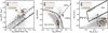 |
Fig. 1. Characterization of the three galaxies presented in this work in terms of stellar mass, SFRs, and AGN activity. Left: SFR–M⋆ plane. The solid and dashed lines represent the main-sequence (MS) parametrization suggested by Whitaker et al. (2012) and the 4 × SFR(MS) starburst threshold, respectively. Middle: BPT-diagram (Baldwin et al. 1981). The dashed curve shows the empirical star-forming threshold (Kauffmann et al. 2003), whereas the solid curve corresponds to the theoretical maximum starburst model (Kewley et al. 2001). These two lines encompass the SFGs-AGN “composite” zone. The dotted-dashed line indicates the division between AGNs and LINERs (Schawinski et al. 2007). Right: WISE mid-IR colour-colour diagram. The solid lines delimit the AGN-zone suggested by Mateos et al. (2012), whereas the dashed line represents the AGN threshold adopted by Stern et al. (2012). The WISE data 1-σ errorbars are smaller than the plotted symbol sizes. The GAMA data are taken from their data-release 3 (GAMA-DR3; Baldry et al. 2018), encompassing galaxies at z < 0.35 (the upper redshift limit for the VALES survey) and with 5-σ or higher flux estimates. These three panels indicate that the three galaxies presented in this work can be classified as starbursts, with one target (HATLAS114625−014511) likely to be classified as an obscured AGN host galaxy. |
Using the Baldwin-Phillips-Terlevich (BPT) diagram (Baldwin et al. 1981), we show that two systems lie just below the limit of the pure star-forming region (Kauffmann et al. 2003). The remaining target (HATLAS114625−014511) is located in the low ionization nuclear emission line region (LINER). The Hβ, [O III], Hα, and [N II] flux measurements are presented in Appendix A. By using the Wide-field Infrared Survey Explorer (WISE; Wright et al. 2010) mid-IR colour diagram (right-hand panel in Fig. 1; Stern et al. 2012; Mateos et al. 2012), HATLAS114625−014511 would be classified as an active galactic nucleus (AGN) host galaxy, while the other two targets are classified as SFGs in agreement with the BPT-diagram analysis.
2.2. ALMA observations
In this work, we describe an ALMA follow-up campaign (taken from project 2015.1.01012.S; P.I.: E. Ibar) for imaging three VALES galaxies for which we obtained the previous bright CO(1–0) detections presented in Villanueva et al. (2017). Observations were taken on Band-3 with the extended 12 m array to obtain higher spatial and spectral resolution imaging than previous observations.
The spectral setup was designed to target the redshifted CO(1–0) emission line (between 97 GHz and 103 GHz, depending on the source) using a spectral window in frequency division mode to cover 1.875 GHz of bandwidth at a native 3906.250 kHz resolution. The other three spectral windows were used in time division mode and were positioned to measure the continuum emission around the redshifted line. Observations were taken under relatively good weather conditions with precipitable water vapour (P.W.V.) ranging from 0.6 mm to 0.8 mm, and using 36 to 38 antennas with a maximum baseline of 1.5 km. The phase, bandpass, and flux calibrations are listed in Table 1.
ALMA observational setup for project 2015.1.01012.S.
Data reduction was carried out using the Common Astronomy Software Applications (CASA) and using the provided ALMA pipeline up to calibrated uv products. Data taken on different days were concatenated together after running the pipeline and before imaging. After exploring different imaging approaches using task TCLEAN, and guided by our scientific objectives, we decided to use a Briggs weighting (ROBUST = 0.4) to reach a major axis full width half maximum (FWHM) for the synthesized beam (θBMAJ) in a range between  . For each source, we applied a slight convolution (within TCLEAN) to obtain a circular beam. The pixel size was set to
  . All three sources were clearly detected at high significance, and the signal was interactively cleaned down to 2−3-σ in spectral channels with confident source emission.
Final images reach rms noises of ∼400−500 μJy beam−1 at ≈12 km s−1 channel width. The channel width was set to minimize spectral resolution effects (Molina et al. 2019a). The continuum emission image, obtained over 6 GHz bandwidth, reaches noise levels of 13 μJy beam−1. Two targets are detected as point sources with peak flux densities of ∼110 μJy beam−1, while HATLASJ121446.4−011155 remains undetected.
2.3. SINFONI observations
We observed the Paα emission line by using the SINFONI IFU (Eisenhauer et al. 2003) on the ESO-VLT in its seeing-limited mode (Project 099.B-0479(A); P.I. J. Molina). The SINFONI field-of-view (FOV) is 8″ × 8″ with a pixel angular size of  . The spectral resolution is λ/Δλ ∼ 3800, and OH sky lines have ∼5 Å FWHM (≈30 km s−1 at 2.1 μm). The observations were carried out in service mode between 2017 March 15 and 2017 December 11 in seeing and photometric conditions (point spread function – PSF
  in K-band). In addition, two different jittering patterns were used during the observing runs in order to boost the observation signal-to-noise ratio (S/N) in one galaxy.
2.3.1. “OSSO” jittering
To observe the HATLASJ1146251−014511 and HATLASJ121446.4−011155 galaxies (hereafter, HATLAS114625 and HATLAS121446, respectively), we used the traditional “ABBA” chop sequences, nodding  across the IFU. That means that the traditional jittering OBJECT-SKY-SKY-OBJECT (“OSSO”) pattern was implemented. We used one observing block (OB) per target, implying a total observing time of ≈3.2 ks per source. The raw datasets for these two sources were reduced by using the standard SINFONI ESOREX1 data reduction pipeline.
2.3.2. OOOO Jittering
We perform an on-source experimental jittering pattern to increase the S/N of the Paα emission line in one galaxy. In this experimental observation, the pointing was kept fixed at the galaxy location. Thus, an OBJECT-OBJECT-OBJECT-OBJECT (“OOOO”) jitter sequence was used. Based on previous analyses by Godoy et al. (in prep.), this observing approach provides reliable results for emission lines with S/N ≳ 15.
To reduce the data, we first used the SINFONI ESOREFLEX and ESOREX pipelines. Then, sky emission lines were subtracted using SKYCOR (Noll et al. 2014), while MOLECFIT (Kausch et al. 2015) was implemented to remove telluric absorption bandpass lines (Godoy et al., in prep.). This was necessary as we did not have “sky” observations.
To test this experimental jitter pattern, we chose the brightest galaxy in our small sample, HATLASJ090750.0+010141 (hereafter, HATLAS090750). By using this method, the observed emission line S/N is expected to increase by  compared to the use of an OSSO jitter pattern due to the extra on-source time. For this observation, the exposure time was also set to ≈3.2 ks. More details about this experimental observation are reported in Appendix B.
2.3.3. Flux calibration
The standard star observation was used to perform the flux calibration. First, the galaxy spectrum was corrected in each pixel by atmospheric telluric absorptions and by the SINFONI K-band transmission curve. We did this by collapsing the standard star datacube in the spectral axis using a wavelength range free from significant telluric absorptions. A two-dimensional Gaussian function was fitted to this spectrally collapsed image. Then, we extracted the spectrum from the standard star by using an aperture size of 2 × FWHM in diameter. We used this standard star spectrum to normalize the galaxy spectrum observed in each pixel. We took into account the different total exposure times.
Then, in each pixel, we multiplied the normalized spectrum by a representative stellar black-body profile. To obtain this black-body curve, we fitted a black-body function to the standard star magnitudes collated in the Visual Observatory SED Analyser (VOSA, Bayo et al. 2008). This allowed us to estimate the stellar surface temperature – thus the black-body function shape – and the normalization constant to construct the representative standard stellar black-body profile as seen in the SINFONI K-band. We note that the typical relative uncertainty for the conversion factor is ∼5% (e.g. Piqueras López et al. 2012).
Even though we can provide reliable flux calibrations for HATLAS114625 and HATLAS121446, the different on-source (OOOO) observing mode for HATLAS090750 impeded a proper calibration from its standard star observation. The flux calibration for this observation requires us to carefully model the sky for the standard star observation and, hence, the stellar spectrum. However, we were unable to obtain an accurate stellar atmospheric model for the standard star (HD 56006) due to its uncertain stellar parameters. More details about these uncertainties are presented in Appendix B.
2.3.4. Spatial resolution
We also used the spectrally collapsed standard star image to determine the PSF FWHM (θPSF) for each K-band observation. By fitting a two-dimensional Gaussian function, we determined  ,
,  , and
, and  for HATLAS090750, HATLAS114625, and HATLAS121446, respectively.
2.4. Stellar mass and IR-based SFR estimates
The stellar masses for the three galaxies were estimated in Villanueva et al. (2017) by using the photometry provided by the GAMA survey (extending from the far-UV to far-IR (FIR) – ∼0.1−500 μm) and by using the Bayesian SED fitting code MAGPHYS (Da Cunha et al. 2008). We assumed a Chabrier (2003) initial mass function (IMF). The M⋆ values are presented in Table 2.
Spatially integrated measurements for the three starbursts.
The IR-based SFRs (SFRFIR) were estimated by using the rest-frame far-IR 8−1000 μm luminosity (LIR) estimates taken from Ibar et al. (2015). By assuming a Chabrier (2003) IMF, the SFRIR values were calculated following SFRIR (M⊙ yr−1) = 10−10 × LIR (L⊙; Kennicutt 1998b) and correspond to the obscured star-formation activity. The IR-based SFRs are consistent with the SFR estimates suggested by MAGPHYS but tend to be offset by a factor of ∼2 towards higher values (see Villanueva et al. 2017 for more details).
2.5. CO(1–0) luminosities
The total galaxy CO(1–0) velocity-integrated flux densities (SCO(1−0)Δv) were taken from Villanueva et al. (2017). Briefly, these were estimated by implementing a two-step procedure. First, the CO(1–0) line was spectrally fitted by a Gaussian profile to determine its FWHM and to spectrally collapse the datacube within ±1 × FWHM. Then, SCO(1−0)Δv values were estimated by fitting a two-dimensional Gaussian function to the spectrally integrated datacube (moment 0) using the task GAUSSFIT within CASA. Finally, the CO(1–0) luminosities ( ) were calculated by following Solomon & Vanden Bout (2005):
![Mathematical equation: $$ \begin{aligned} L^{\prime }_{\rm CO(1{-}0)} = 3.25 \times 10^7\,S_{\rm CO(1{-}0)} \Delta { v}\, \nu _{\rm obs}^{-2}\, D^2_{\rm L}\, (1+z)^{-3}\, \mathrm{[K\,km\,s^{-1}\,pc^2]}, \end{aligned} $$](/articles/aa/full_html/2020/11/aa39008-20/aa39008-20-eq17.gif) (1)
(1)
where SCO(1−0)Δv is in Jy km s−1, νobs is the observed frequency of the emission line in GHz, DL is the luminosity distance in Mpc, and z is the redshift. Both estimates are presented in Table 2.
3. Analysis and results
3.1. Average ISM properties
To analyse the spatially integrated emission line fluxes for our three galaxies, we first collapsed the new ALMA and SINFONI datacubes into one-dimensional spectra (Fig. 2). These spectra were built by stacking the spectra seen in the individual pixels from which we detected an emission line (see Sect. 3.2). Before stacking, we manually shifted the individual emission lines to rest-frame accounting for redshift and the respective pixel line-of-sight (LOS) velocity value (see Fig. 3). Thus, we tried to minimize any line broadening produced by rotational motions, and we focused on intrinsic individual emission line widths.
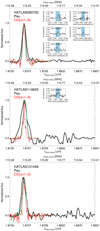 |
Fig. 2. Spatially integrated rest-frame spectra around the emission lines of interest. The bottom and top x-axes show the rest-frame wavelength and frequency ranges for the Paα and CO(1–0) emission lines, respectively. For each galaxy, the solid green curve shows the CO(1–0) spectrum convoluted by the SINFONI LSF. From HATLAS090750, we also detect the Brδ, H2(1–0)S(3), H2(1–0)S(2), H2(1–0)S(1), and He I near-IR emission lines using as an aperture an encircled zone given by the PSF FWHM and centred at the Paα luminosity peak. In the case of the HATLAS114625 galaxy observation, we also detect the H2(1–0)S(3) emission. These detections are shown in the sub-plots (blue-shaded area) in each panel (see also Appendix C). The CO(1–0) and Paα emission lines are clearly detected. |
In all three starbursts, the spatially integrated Paα emission line seems broader than the CO(1–0) emission line. By convolving the ALMA spatially integrated spectrum by the SINFONI line spread function (LSF; green curves in Fig. 2), we find that the spectral resolution difference is not producing this trend. The difference between the spatially integrated Paα and CO(1–0) line widths seems to be caused by broader nuclear Paα emission lines in the individual pixels in each galaxy (see Sect. 3.2.2). The broad nuclear Paα emission lines indicate that the ionized gas ISM phase is more affected by turbulent supersonic motions than the molecular gas2. We do not detect any broad-line component (> 500 km s−1) in the spatially collapsed SINFONI spectra, suggesting the absence of signatures from a broad-line region produced by an AGN.
We used the Paα emission line fluxes to derive SFR estimates (less affected by attenuation compared to Hα) using the Kennicutt (1998b) conversion for the Chabrier (2003) IMF. By assuming an intrinsic Hα-to-Paα ratio equal to 0.116 (Case B recombination, Osterbrock & Ferland 2006), the Paα-based SFRs (SFRPaα) were calculated following SFRPaα (M⊙ yr−1) = 4.0 × 10−41 × LPaα (erg s−1). The SFRPaα values are presented in Table 2. We do not present an SFRPaα estimate for the HATLAS090750 galaxy as we were unable to obtain a reliable flux calibration for its SINFONI observation.
We computed the nebular E(B − V) colour excess (E(B − V)Neb) by using the observed Hα-to-Paα flux ratio3 and assuming a Calzetti et al. (2000) attenuation law. We list the E(B − V)Neb values in Table 2. We note that these E(B − V)Neb values are ∼4.7 and ∼2.3 times higher than the colour excess estimates given by MAGPHYS for the stellar component (E(B − V)⋆ ≈ 0.29 and ≈0.39 for HATLAS114625 and HATLAS121446, respectively). This is expected from local galaxy studies, where the higher E(B − V)Neb values suggest a differential attenuation model in which stars experience attenuation from a diffuse ISM dust component, but the massive young stars experience an additional attenuation as they are embedded in their dusty birth clouds (Calzetti et al. 2000). However, we note that the HATLAS114625 nebular-to-stellar colour excess ratio is twice than the average value found in local galaxies (∼2.3, Calzetti et al. 2000), indicating its highly dusty nature, and more in line with the findings of an extreme obscured starburst galaxy population at z ∼ 0.5−0.9 (Calabrò et al. 2018).
By considering the derived E(B − V)Neb values, we estimated attenuation-corrected SFRPaα (SFRPaα, corr) values of 67 ± 8 and 40 ± 6 M⊙ yr−1 for HATLAS114625 and HATLAS121446, respectively. These estimates are slightly higher than the SFRFIR values (Table 2) but still consistent with the 2-σ uncertainties for both starbursts.
3.2. Galaxy dynamics
We constructed the two-dimensional moment maps by following Swinbank et al. (2012). Briefly, the spectrum associated with each pixel corresponds to the average spectrum calculated from the pixels inside a square area that contains the spatial resolution element – the synthesized beam or PSF. The noise per spectral channel was estimated from a region that does not contain any source emission. We used the LMFIT PYTHON package (Newville et al. 2014) to fit a Gaussian profile to the emission lines. In the case of the SINFONI observations, we masked the spectrum at the wavelength ranges where OH sky-line features are present, and the Paα line widths were corrected by spectral resolution effects. We applied an S/N = 5 threshold to determine whether we have detected an emission line or not. If this criterion was not achieved, then we increased the square binned area by one pixel per side and repeated the Gaussian fit. We iterated up to two more times in order to avoid large binned regions. After the third iteration, if the S/N criterion was not achieved, we masked that pixel and skipped to the next one.
The pixel-by-pixel intensity, velocity, and velocity dispersion 1-σ uncertainties were estimated by re-sampling via Monte Carlo simulations the flux density uncertainties in the data. The maps from both emission lines are presented in Fig. 3.
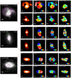 |
Fig. 3. K-band, intensity, velocity, velocity dispersion, and residual maps (first to fifth columns) for HATLAS090750 (top), HATLAS114625 (middle), and HATLAS121446 (bottom). For each galaxy, from the second column to the last column, we show the Paα and CO(1–0) two-dimensional maps, one above the other, respectively. The spatial scale for each observation is shown in each map. The K-band map has the CO(1–0) and Paα emissions over-plotted in green and pink contours, respectively. The CO(1–0) intensity map shows the synthesized beam size. In the velocity and velocity dispersion maps, the white cross indicates the location of the best-fitted dynamical centre. The velocity maps have the velocity contours over-plotted from their best-fit disc models, and the green- and pink-dashed lines represent the molecular and ionized gas major kinematic axes, respectively. In each velocity dispersion map, the white circumference represents the boundary of the region masked during the estimation of the global velocity dispersion value. The residual fields are constructed by subtracting the velocity disc models from the velocity maps. The rms of these residuals are given in each panel. In the case of the HATLAS090750 Paα observation, we only show the modelled central zone in the residual map. |
The CO(1–0) and Paα intensity maps present smooth distributions with no clear level of clumpiness, at ∼kpc-scales, in the three starbursts. These also agree with the stellar morphology seen in the K-band image. However, we note that OH sky-line features present in the SINFONI observations may add noise to the Paα two-dimensional maps, and this may partly explain the smoother CO(1–0) maps as the ALMA spectra are free from sky-line residuals.
In the particular case of the HATLAS090750 system, the K-band and Paα intensity images show two asymmetric features that may be related to gas inflow, gas outflow or tidal interaction. These features suggest an ongoing merging process. Both features account for ∼18% of the total Paα flux suggesting ongoing star-formation activity. One of the asymmetric features has a projected velocity blueshift of ∼ − 300 km s−1 compared to the system centre, while the other feature presents a velocity redshift of ∼80 km s−1, suggesting that this system has a complex three-dimensional shape. The ALMA observation just traces the CO(1–0) emission coming from the central part of this system, probably due to sensitivity limitations. Interestingly, the central part of this system shows a rotational pattern in the CO(1–0) and Paα velocity maps, with a peak-to-peak rotational velocity of Vmaxsin(i) ∼ 90 km s−1.
In contrast, HATLAS114625 and HATLAS121446 show clear disc-like rotational patterns in their CO(1–0) and Paα velocity maps. The ionized and molecular gas kinematics broadly agree in both starbursts, with peak-to-peak rotational velocities of Vmaxsin(i) ∼ 360−460 km s−1, respectively.
3.2.1. Kinematic modelling
We modelled the ionized and molecular gas ISM kinematics by fitting the two-dimensional LOS velocity fields. The model velocity maps were constructed by assuming an input arctan rotation curve:
 (2)
(2)
where Rt is the radius at which the rotation curve turns over, V0 is the systemic velocity (i.e. redshift), and Vasym is the asymptotic rotational velocity (Courteau 1997).
For each observation, the kinematic model considers seven free parameters (V0, Vasym, Rt, PA, [x/y], and inclination angle). We convolved the velocity model map with the PSF or synthesized beam, and we used the EMCEE PYTHON package (Foreman-Mackey et al. 2013) to find the best-fit model.
We used the K-band Sérsic photometric models (Sérsic 1963) to constrain the inclination angle values. We used the K-band best-fit minor-to-major axis ratio (b/a; Table 3) as initial guess inputs to the kinematic modelling, and we allowed it to search the best-fit inclination value within a 3-σ range. To better account for the K-band model b/a uncertainty, we adopted a b/a ratio 1-σ relative error equal to 10%, as suggested by Epinat et al. (2012). The inclination angle was derived from b/a by considering an oblate spheroid geometry (Holmberg 1958):
 (3)
(3)
K-band surface brightness Sérsic best-fit model parameters taken from the GAMA-DR3 for our sample (Kelvin et al. 2012).
where “i” is the galaxy inclination angle and q0 is the intrinsic minor-to-major axis ratio (i.e. disc thickness) of the galaxy. For edge-on systems (i = 90 deg), q0 = b/a. We used the q0 = 0.14 mean value reported for edge-on galaxies at low redshift (z < 0.05, Mosenkov et al. 2015).
The model best-fit parameters and  values are given in Table 4, and the rms values are shown in each residual map (Fig. 3). The kinematic position angles roughly agree with each other (ΔPA = PAPaα − PACO ≲ 10 deg). For the HATLAS114625 and HATLAS121446 galaxies, these also roughly agree with the position angles derived from the K-band image modelling.
Best-fit kinematic parameters for the galaxies in our sample.
The best-fit disc model gives a reasonable fit to the inner ionized and molecular gas kinematics of the HATLAS090750 galaxy, as suggested by the low reported rms value. This may indicate a fast relaxation process of the ISM molecular gaseous phase into a disc-like galaxy in the central zone of this system (e.g. Kronberger et al. 2007). For the other two galaxies, the rms values presented in the Paα velocity residual maps tend to be larger than the values derived from the CO(1–0) observations, suggesting that the ionized gas ISM phase may be a more sensitive tracer of non-circular motions compared to the molecular gas ISM phase. However, these high rms values are also a consequence of the coarser SINFONI spectral resolution compared to the ALMA observations as well as additional noise induced by the OH sky-line features present in some pixels at the wavelengths where the Paα emission line is found.
3.2.2. Kinematic parameters
We used the best-fit dynamical models to simulate a slit observation along the major kinematic axis, and we extracted the one-dimensional rotation velocity and velocity dispersion curves for both ISM phases (Fig. 4). We considered a slit width equal to the synthesized beam or PSF FWHM. The half-light radii for the ionized and molecular gas ISM phases (R1/2, Paα, R1/2, CO) were calculated by using a tilted ring approach. From the rotation curve, we defined the rotational velocity for the Paα and CO observations (Vrot, Paα, Vrot, CO) as the inclination-corrected values observed at two times the Paα and CO half-light radii, respectively.
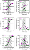 |
Fig. 4. Rotation velocity (left) and velocity dispersion (right) profiles across the major kinematic axis for the HATLAS090750 (top), HATLAS114625 (middle), and HATLAS121446 (bottom) galaxies. The errorbars show the 1-σ uncertainties. The vertical black-dashed line represents the best-fit dynamical centre. The light grey shaded area represents the 3× synthesized beam size region centred at the best-fit molecular gas dynamical centre, whereas the dark grey dashed area represents the 3× PSF FWHM zone centred at the best-fit ionized gas dynamical centre. In the rotation velocity profile panels, the dashed-magenta and solid-green curves show the rotation curves extracted from the beam-smeared Paα and CO(1–0) two-dimensional best-fit models, respectively. In the velocity dispersion profile panels, the green- and magenta-dashed lines show the median galactic value estimated from the outskirts of the galactic disc (Table 4) for the CO(1–0) and Paα observations, respectively. We find a good agreement between the rotation curves derived from the ionized and molecular gas ISM phases in the three starbursts. |
To correct the velocity dispersion values for beam-smearing effects, we applied the correction suggested by Stott et al. (2016). This corresponds to a linear subtraction of the local velocity gradient ΔV/ΔR from the beam-smeared line widths. However, to further consider beam-smearing residual effects from this correction, we defined the global velocity dispersion for each gas phase (σv, CO, σv, Paα) as the median value taken from the pixels located beyond three times the synthesized beam or PSF FWHM from the dynamical centre (white circumferences in velocity dispersion maps in Fig. 3).
For HATLAS090750, we find a very compact CO light distribution, as suggested by its half-light radius. In its central zone, this system shows a low rotational velocity value (Vrot, CO ∼ 70 km s−1) and a high median velocity dispersion σv, CO ∼ 35 km s−1, suggesting a molecular gas ISM phase with highly supersonic turbulent motions and a CO-traced kinematic ratio Vrot, CO/σv, CO ∼ 2. The CO- and Paα-based rotation curves clearly agree at the radius at which CO(1–0) is detected (Fig. 4), implying that the Vrot, CO and Vrot, Paα values also agree.
In contrast, the Paα emission tends to show broader line widths compared to the CO emission line (σv, Paα ∼ 66 km s−1). This is unlikely to be produced by beam-smeared flux coming from the asymmetric features as the broader Paα line widths are seen across the entirety of the major kinematic axis. Assuming that the line widths trace the turbulent kinematic state of the respective ISM gas phase, this result suggests that the molecular gas phase may be able to dissipate the turbulent kinetic energy faster than the ionized gas phase. Another possibility could be an additional energy injection in the ionized gas from stellar feedback such as stellar winds, supernovae feedback, and/or Wolf-Rayet episodes (e.g. Thornton et al. 1998; Crowther 2007; Kim & Ostriker 2015; Martizzi et al. 2015; Kim et al. 2017). The expansion of over-pressured H II regions is also a possibility (Elmegreen & Scalo 2004). We recall that we have corrected the SINFONI observations by using instrumental line broadening effects.
For HATLAS114625 and HATLAS121446, the molecular and ionized gas ISM phases show similar scale sizes R1/2, Paα/R1/2, CO ≈ 0.85 ± 0.01 and 0.96 ± 0.01, respectively. For HATLAS121446, these half-light radius estimates also agree with R1/2, K (see Table 3). However, for HATLAS114625, we find that R1/2, K/R1/2, CO/Paα ≈ 1.3−1.6 kpc, suggesting that the ionized and molecular gas ISM phases are distributed in a more compact disc-like structure in this galaxy.
For both starbursts, the velocity curves agree, and we derived ionized to molecular gas rotation velocity ratios Vrot, Paα/Vrot, CO ≈ 1.04 ± 0.04 and 0.94 ± 0.14 for HATLAS121446 and HATLAS114625, respectively. The consistency between the CO- and Hα-based velocity curves tends to be found in local galaxies where the ionized gas emission seems to come from recent star-formation activity episodes (Levy et al. 2018).
In both systems, the median σv, CO values are lower than the corresponding σv, Paα estimates (σv, Paα/σv, CO ∼ 1.5−2); however, they still agree within 1-σ uncertainties. The CO and Paα velocity dispersion values seen in both galaxies suggest a dominant common nature. The CO and Paα velocity dispersion profiles (Fig. 4) suggests even closer σv, Paα and σv, CO values. Nevertheless, we note that our measured σv, CO values tend to be higher than the estimates reported from local systems (≈9−19 km s−1, Levy et al. 2018). Indeed, these median σv, CO values are consistent with the lower end of the velocity dispersion estimates measured from ULIRGs (∼30−140 km s−1, Downes & Solomon 1998; Wilson et al. 2019).
We derive an average CO-based rotational velocity to dispersion velocity ratio (Vrot, CO/σv, CO) of 8 ± 3 and 7 ± 2 for HATLAS114625 and HATLAS121446, respectively. If we consider the Paα observations, we derive Vrot, Paα/σv, Paα ∼ 4 ± 2 and ∼5 ± 3, respectively. Independent of the emission line considered, the Vrot/σv ratios measured for HATLAS114625 and HATLAS121446 suggest that the rotational motions are the main support against self-gravity in both starburst galaxies.
3.2.3. Comparison with previous VALES works
Using our kpc-scale resolution data ( ), we tried to test if the previous kinematic analysis done for the VALES galaxies (Molina et al. 2019a) may be biased due to beam-smearing effects. These previous CO(1–0) observations were performed by using a more compact ALMA array configuration, thereby delivering a coarser spatial resolution (∼3−4″ ≈ 5−7 kpc). Beam-smearing could hide galaxy morpho-kinematic properties, making it hard to recover unbiased intrinsic parameters when the spatial resolution is of the order of several kpc.
The galaxies presented in this work, HATLAS114625 and HATLAS121446, were not described in Molina et al. (2019a) as they were not extended enough for a dynamical interpretation. However, we can still make a brief comparison with the VALES systems that share similar global properties.
We concentrated on VALES sources with specific SFR values (sSFR ≡ SFR/M⋆; Δlog(sSFR) < 0.3 dex) similar to those estimated for HATLAS114625 and HATLAS121446 (sSFR = 10−100 Gyr, respectively). For these sources, we find that the kinematic maps present marginally resolved rotation (Vrot, CO ≈ 40−200 km s−1) and high velocity dispersion values (σv, CO ≈ 40−70 km s−1), implying Vrot, CO/σv, CO ratios in the range of 1−3. These values are lower than the ones presented in this work, suggesting that the kinematic parameters presented in Molina et al. (2019a) might be systematically biased due to beam smearing. This comparison is not straightforward as the resolution presented in this work is five to seven times higher than in Molina et al. (2019a); however, it highlights the importance of high-resolution imaging for extracting more precise dynamical information.
3.3. The CO-to-H2 conversion factor from dynamics
A CO-to-H2 conversion factor must be used to estimate molecular gas masses from the CO luminosities ( , e.g. Bolatto et al. 2013). Traditionally, two different αCO values have been considered to calculate MH2 for galaxies as a whole (Solomon & Vanden Bout 2005). An αCO, MW ≈ 4.6 M⊙ (K km s−1 pc2)−1 value seems to be more appropriate for disc-like galaxies (e.g. Solomon et al. 1987), whereas an αCO, ULIRG ≈ 0.8 M⊙ (K km s−1 pc2)−1 value has been estimated for ULIRGs and assumed to be representative for merger-like systems (e.g. Downes & Solomon 1998). However, it is unlikely that αCO follows a bi-modal distribution. Models suggest a smooth transition that depends on the ISM physical properties (e.g. Narayanan et al. 2012).
We exploited the dynamical mass estimate [ ] to constrain the αCO value. In this procedure, we assumed that the dynamical mass estimate corresponds to the sum of the stellar, molecular, and dark matter masses (e.g. Motta et al. 2018; Molina et al. 2019b). This is true when looking at the central regions of galaxies. The HI component at larger scales dominates the gas mass, while the ionized gas might have a role as well. Additionally, for the sake of simplicity, we also assumed a constant αCO value across each galactic disc. Therefore, by quantifying the dark matter content in terms of the dark matter fraction (fDM) at each galactocentric radius, we obtain the following constraint;
 (4)
(4)
where the CO luminosities inside each radius are calculated directly from the ALMA observations, and the stellar masses are truncated using the K-band Sérsic model profile following Molina et al. (2019b).
To estimate the dynamical mass values and use Eq. (4), we first needed to calculate the circular velocity Vcirc at each galactocentric radius. To do this, we considered two cases, the thin- and thick-disc hydrostatic equilibrium approximations. In the first case, the galaxy support against self-gravity is assumed to be purely rotational, and Vcirc corresponds to the observed rotational velocity (Vcirc = Vrot, CO, Genzel et al. 2015). In the second case, the galaxy scale height cannot be neglected, and the self-gravity is balanced by the joint support between the rotational motions and the pressure gradient across the galactic disc (Burkert et al. 2010).
In this “thick-disc” approximation, an analytic expression for Vcirc can be derived by parameterizing the pressure gradients in terms of σv (which is assumed to be constant across the galactic height and radius) and the mass distribution, which we assumed followed the best-fit Sérsic model of the K-band surface brightness distribution:
 (5)
(5)
where Vrot, CO(R) is the rotation velocity profile (Fig. 4) and bnS is the Sérsic coefficient that sets R1/2, K as the K-band half-light radius (e.g. Burkert et al. 2016; Lang et al. 2017; Molina et al. 2019a).
The disc radial coordinates are determined by the best-fit two-dimensional model. Additionally, to minimize beam-smearing effects, we only considered the Vrot, CO values extracted from a zone beyond three times the synthesized beam FWHM from the dynamical centre (see “σv” panels in Fig. 3). However, as we still expected some residual beam-smearing effect at these radii, we also applied a correction factor (≲10%) to the rotation velocity values based on the ratio between the intrinsic-to-smoothed best-fit arctan velocity models across the galaxy major kinematic axis (Appendix D).
We note that this method suffers from a degeneracy between the αCO and fDM(R) parameters; along with it, there is a strong dependence on the accuracy of the Mdyn and M⋆ values. To try to overcome these issues, we used the Markov chain Monte Carlo (MCMC) technique (Calistro Rivera et al. 2018; Molina et al. 2019b) implemented in EMCEE (Foreman-Mackey et al. 2013). We estimated the posterior probability density function (PDF) for the CO-to-H2 conversion factor and the dark matter fraction parameters by sampling the αCO − fDM(R) phase-space defined in Eq. (4) and by considering the likelihood of the estimated  , Mdyn and M⋆ values.
In addition to the thin- and thick-disc dynamical model assumptions, we explored the effect of the chosen underlying mass distribution by assuming that the galaxies follow an exponential total-mass surface density distribution (Freeman 1970). We note that this assumption produces a variation in our thick-disc Mdyn and truncated M⋆ estimates. Thus, we employed a total of four different dynamical models per galaxy.
We did not derive an αCO value for the HATLAS090750 system. This is because this ongoing merger may not fulfil the virial assumption necessary to obtain a dynamical mass estimate.
In Fig. 5, we show the αCO posterior PDFs for the HATLAS114750 and HATLAS121664 starbursts. We note that the thick-disc Sérsic mass-profile model suggests slightly higher αCO values than the other three models for both galaxies. This is produced by two effects; (1) the additional pressure gradient support against self-gravity, which is low for our galaxies as suggested by the Vrot, CO/σv, CO ∼ 7 ratios; and (2) surface density profiles steeper than the ones derived from an exponential model profile as indicated by the Sérsic indices nS ≳ 1. This tends to increase the Mdyn values by a larger amount compared to the truncated M⋆ values at smaller galactocentric radii.
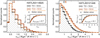 |
Fig. 5. Posterior αCO PDFs for HATLAS114625 (left) and HATLAS121446 (right) starbursts. For each galaxy, we consider four dynamical mass models encompassing different underlying surface density mass distributions and hydrostatic equilibrium approximations. We also show the cumulative probability distribution in each panel with our αCO upper limit defined as P(x < αCO, uplim) ≈ 0.997 (i.e. 3-σ) and estimated by using the thick-disc plus Sérsic dynamical mass model. The coloured arrows indicate the median αCO value for each PDF. We find median αCO estimates consistent with the ULIRG-like value for both starburst galaxies. |
We note that a possible systematic overestimation of M⋆ by MAGPHYS may bias the αCO estimates towards lower values than the reported ones. This scenario is unlikely as we have input a large wavelength SED coverage (∼0.1−500 μm) to obtain accurate M⋆ values (see also Michałowski et al. 2014). However, to be conservative, we assumed the αCO upper limit values (αCO, uplim) given by the PDFs 3-σ range. We obtain αCO, uplim = 2.7 and 5.1 M⊙ (K km s−1 pc2)−1 for HATLAS114625 and HATLAS121446, respectively.
In the remainder of this work, we estimate the molecular gas masses by adopting the median CO-to-H2 conversion factor value derived from the thick-disc Sérsic mass-profile dynamical model, that is, by considering the model that suggests the higher median αCO value. This election does not affect our results as the differences between the four dynamical models are marginal compared to the uncertainties behind the galaxy estimates as seen by the broad αCO PDFs. Our analysis suggests low αCO values that are consistent with the ULIRG-like value for both starbursts. We present this value along with the molecular gas estimates in Table 5.
CO-to-H2 conversion factor, molecular gas masses, and gas fractions for HATLAS114625 and HATLAS121446 starbursts.
A direct result of adopting that αCO value is that our early expectation about observing gas-rich systems was wrong. Indeed, the measured fH2 values are consistent with the average estimate for local SFGs (fH2 ∼ 0.1, Leroy et al. 2009; Saintonge et al. 2017). This suggests that these starburst galaxies may not be gas-rich, as originally expected, implying that without a robust molecular gas estimate, it is not straightforward to catalogue these systems as possible analogues of the high-z SFG population.
4. Discussion
4.1. What sets the molecular gas velocity dispersions?
HATLAS114625 and HATLAS121446 present σv, CO values that are comparable with the lower end estimates observed in ULIRGs (σv, CO ≈ 30−140 km s−1, Downes & Solomon 1998; Wilson et al. 2019). However, both galaxies show regular disc-like kinematics with little evidence of interactions that may enhance the internal σv, CO values, suggesting that the high molecular gas velocity dispersion values may be produced by internal secular processes.
Wilson et al. (2019) found that, in ULIRGs, the σv, CO values roughly increase with the molecular surface density (ΣH2), following a power-law relationship with a tentative exponent of ∼0.5. Wilson et al. (2019) suggested that this correlation can be explained if ULIRGs are in vertical pressure balance. In this section, we explore whether or not their model is able to explain the σv, CO values measured for the HATLAS114625 and HATLAS121446 galaxies. We chose the ISM pressure balance model from Wilson et al. (2019) because we lack the stellar velocity dispersion measurement for our sources. This quantity is required to calculate the pressure set by self-gravity in other ISM models such as, for example, the traditional Elmegreen (1989) ISM model.
In the Wilson et al. (2019) model, a downwards pressure on the molecular gas (modelled as a gas layer) is produced by the disc self-gravity plus an additional contribution from the dark matter halo. This pressure can be calculated as:
 (6)
(6)
where ΣTot is the disc total-mass surface density and γ is a factor that accounts for the vertical pull towards the galaxy mid-plane produced by dark matter. This factor depends inversely on Vrot/σv squared, thus it contributes a small correction for both galaxies (γ ∼ 0.05).
The upwards pressure is parameterized as a function of the average mid-plane density ρmid and the thermal plus turbulent velocity dispersions:
 (7)
(7)
where ρmid = ΣH2/2hH2, hH2 is the molecular gas disc scale height, σv, H2 is the molecular gas velocity dispersion (hereafter we assume σv, H2 ≈ σv, CO), and ψ is a factor that accounts principally for the magnetic-to-thermal support ratio (∼0.3, Kim & Ostriker 2015) as the cosmic ray-to-turbulent support ratio is negligible (see Wilson et al. 2019 for more details).
The vertical equilibrium condition requires Pgrav, W + 19 = PISM and allows us to write Eq. (6) from Wilson et al. (2019) in a more compact form:
 (8)
(8)
From this equation, if galaxies have similar ΣH2/ΣTot ratios, then  , and hH2 is constant across the galactic radius, that is, the correlation found by Wilson et al. (2019) for local ULIRGs.
In the left-hand panel of Fig. 6, we plot the pixel-by-pixel σv, CO values as a function of ΣH2 (corrected by projection effects) for HATLAS114625 and HATLAS121446. All the values associated with the pixels that reside inside the central galactic region4 are shown in grey, highlighting that these σv, CO values are likely to be overestimated due to beam-smearing residual effects.
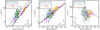 |
Fig. 6. Left: pixel-by-pixel molecular gas velocity dispersion estimates as a function of molecular gas surface density. For each starburst galaxy, in grey, we show the σv, CO values that may be overestimated due to beam-smearing residual effects. The errorbar in the lower-right corner indicates the typical 1-σ uncertainty, whereas the arrow represents the systematic uncertainty given by the use of our αCO upper limit instead of the adopted value. The “z ∼ 0 ULIRG” sample is taken from Wilson et al. (2019). The “z ∼ 0 SFGs” sample estimates are galactic average values measured for a sub-sample of galaxies taken from the CARMA-EDGE survey (Bolatto et al. 2017; Levy et al. 2018). The “z ∼ 1.5 SFG” data correspond to the ∼kpc-scale measurements for a main-sequence galaxy presented in Molina et al. (2019b). The solid line represents the empirical relationship suggested by Wilson et al. (2019). The dashed line shows the empirical relationship corrected by the average ΣH2/ΣTot and Vrot, CO/σv, CO ratios measured for both systems. Middle: pixel-by-pixel σv, CO values as a function of the total surface density. Right: molecular gas scale height as a function of the total gas surface density. The last two panels are colour-coded in the same way as the left panel. The vertical pressure equilibrium model gives a reasonable representation of our data. |
We also show the values presented by Wilson et al. (2019) for the local ULIRG sample (measured at 450−650 pc scales) and the average galactic values for a sub-sample of 17 SFGs taken from the EDGE-CALIFA survey (Bolatto et al. 2017). For these SFGs, the σv, CO values are taken from Levy et al. (2018), whereas the average ΣH2 values are calculated by using the MH2 and R1/2,CO estimates presented in Bolatto et al. (2017) and assuming a radial spatial extension of 2 × R1/2,CO. The “z ∼ 1.5” SFG data correspond to ∼kpc-scale measurements for a main-sequence galaxy presented in Molina et al. (2019b).
Despite comparing data observed at different spatial resolutions, both starbursts exhibit σv,CO values mainly in the range between the local SFGs and ULIRGs, but their ∼kpc-scale ΣH2 values are comparable to the average estimates measured for the local SFGs and much lower than the estimates reported for the ULIRG sample. However, similar to the ULIRGs, the starburst data seem to follow a roughly  power-law relationship. This is shown by the dashed line that represents the pressure balance model suggested by Wilson et al. (2019) but scaled to the average ΣH2/ΣTot and Vrot, CO/σv, CO ratios measured for both systems. Additionally, the solid line shows the Wilson et al. (2019) model for the local ULIRGs.
We now consider the total surface density ΣTot (Fig. 6). We approximated ΣTot by the sum of ΣH2 and the stellar surface density Σ⋆ (ΣTot ≡ ΣH2 + Σ⋆). For each starburst, the pixel-by-pixel Σ⋆ values were calculated by scaling the SINFONI K-band continuum image surface brightness distribution (Fig. E.1) to the global M⋆ value derived by MAGPHYS.
The HATLAS114625 and HATLAS121446 starbursts tend to be located in the lower ΣTot limit covered by the ULIRG sample. Despite of the large scatter (≈0.22 dex for non-masked values), the vertical pressure balance model (solid line) gives a reasonable representation of the data. We note that the systematic uncertainty added by the adopted αCO conversion factor is low since the ΣTot values are mainly dictated by Σ⋆ in both starbursts (sources have low integrated molecular gas fractions; see Table 5). The scatter is probably increased by the use of a constant mass-to-light ratio to estimate Σ⋆.
By using Eq. (8), we roughly estimated hH2 for both starbursts. We plot the hH2 pixel-by-pixel distribution in the right-hand panel of Fig. 6. From the non-masked pixels, we obtain  and
and  pc median values for HATLAS114625 and HATLAS121446, respectively. Those values are consistent with the average estimate reported for the ULIRG systems (∼150 pc; Wilson et al. 2019). Our data support the scenario in which the molecular gas velocity dispersion on large scales (∼kpc-scales) is set by the local gravitational potential of the galaxy through the reaching of the vertical pressure balance as suggested by Wilson et al. (2019).
We note that the main difference between the two starbursts analysed in this work and the ULIRGs presented by Wilson et al. (2019) is that, in the former, the vertical gravitational pressure is mainly dictated by the stellar component (fH2 ∼ 0.1) and not by a nearly equal gravitational contribution from stars and gas. Indeed, if in Eq. (6) we take the approximation ΣTot ∼ Σ⋆ and we assume vertical pressure equilibrium, then we obtain  , suggesting that, even in starburst systems, the molecular gas dynamical properties can be set by the stellar gravity.
Momentum injected by stellar feedback may be insufficient to produce the observed σv, CO − ΣTot trend. Hydrodynamical simulations suggest that stellar feedback can only account for σv values up to ∼6−10 km s−1 for the diffuse gas component and that the σv values increase moderately with respect to gas surface density (Ostriker & Shetty 2011; Shetty & Ostriker 2012). However, our data sample the σv, CO ≳ 15 km s−1 range, and additional pressure sources, such as stellar feedback, may still set the σv, CO values below this limit.
Resolution effects should be present as our ∼kpc-scale measurements may underestimate the ambient pressure at smaller scales. This effect has been measured recently by high-resolution (∼60 pc) molecular gas observations in nearby galaxies (Sun et al. 2020). Indeed, Sun et al. (2020) suggest a correction for the ∼kpc-scale pressure estimates. However, their observations cover a considerably lower galactic pressure range (∼104−6/kB K cm−3, see Fig. 8) and, thus, extrapolating such a correction and applying it to our measurements is uncertain. Nevertheless, these high-resolution observations also suggest that the molecular gas is in pressure balance with its weight and the local ISM self-gravity (see also Schruba et al. 2019).
Another major caveat in our analysis comes from the assumption behind Eq. (6). This equation corresponds to a corrected form of the Spitzer (1942) formula for an isothermal layer embedded in a spherical mass component. It does not consider a multi-component composition of the ISM and may not be appropriate to describe the vertical pressure produced by a gaseous plus stellar ISM. For example, in the traditional Elmegreen (1989) ISM pressure formula, the Σ⋆ term is weighted by the ratio between the molecular-to-stellar velocity dispersions (s ≡ σv, CO/σv, ⋆)5. In this case, the additional vertical pressure set by Σ⋆ can be neglected in the limit s ≪ 1. Only if s ∼ 1 is Eq. (6) recovered. Thus, Eq. (6) should be considered as an upper limit case of the Elmegreen (1989) formula.
4.2. The star-formation activity traced at ∼kpc-scales
Our CO(1–0) and Paα observations are ideal for studying the star-formation activity in dusty starburst galaxies. The CO(1–0) emission provides a direct estimate of the molecular gas mass (albeit an αCO), and Paα does not suffer from significant extinction (compared to Hα), facilitating a direct view to the star-formation activity in dustier environments.
The star-formation activity can be described as a power-law relationship between the SFR surface density (ΣSFR) and total gas surface density (Σgas) or ΣH2, the well-known Kennicutt-Schmidt relationship (Kennicutt 1998a). For typical local SFGs, when ΣH2 is used, it is well characterized by a linear relation with an observed average molecular gas depletion time τdep ≡ ΣH2/ΣSFR = 2.2 ± 0.3 Gyr (Leroy et al. 2013). However, this linear trend seems not to be followed by galaxies with enhanced SFRs as those tend to exhibit shorter molecular gas depletion times or higher star-formation efficiencies ( , e.g. Daddi et al. 2010).
In Fig. 7, we show the pixel-by-pixel distribution in the ΣSFR − ΣH2 plane for HATLAS114625 and HATLAS121446. The ΣSFR and ΣH2 quantities are directly estimated from the spatially resolved SINFONI and ALMA observations, assuming the median αCO value (Table 5) and employing the dynamical modelling to correct for projection effects.
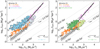 |
Fig. 7. ΣSFR against ΣH2 for the HATLAS114625 (left) and HATLAS121446 (right) starbursts. In each panel, the errorbar in the bottom-right corner represents the typical 1-σ uncertainty. The arrow indicates the horizontal shift of the data produced if we assume the αCO, uplim value instead of the median αCO estimate to calculate ΣH2. This is also highlighted by the lightly coloured data showed in the background. The dotted lines indicate fixed τdep values. We show ∼kpc-scale spatially resolved observations of two z ∼ 0 LIRGs (orange diamonds, Espada et al. 2018) and the median trend observed for the nearby HERACLES galaxy survey (open circles, Leroy et al. 2013). The dot-dashed line represents the best fit for the HERACLES ∼kpc-scale median values. We also present spatially resolved estimates for local ULIRGs measured at ∼350−650 pc scales (Wilson et al. 2019). In solid and dashed lines, we show the double and single power-law best fits reported by Wilson et al. (2019) for the ULIRG data, respectively. Independent of the αCO value assumed, we find lower τdep values than those measured from local normal SFGs. |
We used the HASTROM task written in the Interactive Data Language (IDL) to register the images on the same pixel scales and orientation. While implementing this routine, we considered that the total flux is conserved in each map. We preferred not to include the HATLAS090750 system in our analysis due to its complex geometry and uncertain αCO value.
We compared our ΣSFR − ΣH2 estimates with ∼kpc-scale local galaxy measurements and the ∼sub-kpc data from local ULIRGs. Briefly, the ∼kpc-scale data are represented by the median trend reported from the HERA CO-Line Extragalactic Survey (HERACLES, Leroy et al. 2008) for normal star-forming systems and measurements from two LIRGs (NGC 3110 and NGC 232; Espada et al. 2018). The local ULIRG data correspond to the CO(1–0)-based ∼350−650 pc-scale estimates presented in Wilson et al. (2019).
The two galaxies presented in this work exhibit τdep values in the range of ∼0.1−1 Gyr, that is, τdep values comparable to those derived for ULIRGs (τdep ≲ 0.1 Gyr) but in a low ΣH2 environment. The τdep internal galactic trends are not clear due to the considerable data scatter.
If we assume our αCO, uplim estimates, we obtain τdep median values of ∼0.5 and 0.6 Gyr for HATLAS114625 and HATLAS121446, respectively. In this case, both starbursts mainly present τdep values within 0.2−2.2 Gyr, a range similar to that reported for the two local LIRGs (0.2−1.6 Gyr; Espada et al. 2018). In any case, the depletion times estimated for both galaxies are lower than the τdep median values reported for local SFGs with similar ΣH2 and fH2 values (Leroy et al. 2013). This suggests that the enhancement of the SFE seen in starburst galaxies may not be only related to high ΣH2 estimates.
4.3. Pressure regulated star-formation activity
If star-formation activity also depends on the dynamics of the molecular gas, then ΣSFR should also correlate with the physical variables that regulate these properties. Thus, if the vertical pressure equilibrium sets the molecular gas properties on larger scales (∼kpc-scales, Sect. 4.1), then ΣSFR should correlate with the ISM pressure set by self-gravity Pgrav. The correlation between ΣSFR and ISM pressure has been suggested and observed previously by many authors (e.g. Genzel et al. 2010; Ostriker et al. 2010; Ostriker & Shetty 2011; Bolatto et al. 2017; Herrera-Camus et al. 2017; Fisher et al. 2019) and also used to explain the so-called extended Kennicutt-Schmidt relation (Shi et al. 2011). Indeed, the mid-plane hydrostatic pressure seems to predict the SFE better than gas surface density in atomic-dominated regimes (Leroy et al. 2008).
In Fig. 8, we show ΣSFR as a function Pgrav. The Physics at High Angular resolution in Nearby Galaxies (PHANGS; Leroy et al., in prep.) data correspond to measurements from 28 nearby galaxies presented in Sun et al. (2020) and artificially convolved to a kpc-scale by them. We also consider the spatially resolved ULIRG data presented in Wilson et al. (2019) and The H I Nearby Galaxy Survey (THINGS; Walter et al. 2008; de Blok et al. 2008) and DYNAMO (Green et al. 2014) galactic averages presented in Fisher et al. (2019). We caution, however, that the DYNAMO pressure data are based on ionized gas velocity dispersions and unresolved CO emission line measurements, while we are using spatially resolved molecular gas estimates. We also show the ∼kpc-scale data measured for a typical SFG at z ∼ 1.5 (Molina et al. 2019b).
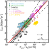 |
Fig. 8. ΣSFR against the ISM pressure set by self-gravity. The PHANGS data correspond to the manually convolved kpc-scale measurements reported by Sun et al. (2020) for 28 nearby galaxies. The ULIRG data correspond to the values measured at ∼350−650 pc scales by Wilson et al. (2019). The DYNAMO data are based on galactic ionized gas velocity dispersion measurements along with spatially unresolved molecular gas observations (Fisher et al. 2019). We also present the ∼kpc-scale values measured for a typical SFG at z ∼ 1.5 (SHiZELS-19; Molina et al. 2019b). The dashed line corresponds to the best fit presented by Fisher et al. (2019) for the DYNAMO and THINGS data, while the solid black line corresponds to the best fit given by Sun et al. (2020) to the PHANGS data. The dot-dashed line corresponds to the parametrization given by Kim et al. (2013) for their set of hydrodynamical simulations. The solid red line represents our best fit. The starburst and ULIRG data are consistent with the trend reported from the nearby galaxies. The z ∼ 1.5 SFG data are in clear offset. |
Our data clearly fill the gap between the ULIRG the PHANGS data in terms of pressure set by self-gravity. We find that ΣSFR is correlated with Pgrav across nearly seven and six orders of magnitude in terms of Pgrav and ΣSFR, respectively.
By performing a linear fit in the log-log parameter space (log10(ΣSFR) = N × log10(Pgrav/P0)) using EMCEE (Foreman-Mackey et al. 2013), we find a best-fit slope N = 0.78 ± 0.01 with an interceptor value log10(P0/kB[cm−3 K]) = 5.38 ± 0.04. This is represented by the red solid line in Fig. 8. In this fitting procedure, we adopted conservative 0.2 dex uncertainties for the PHANGS data estimates (Sun et al. 2020), and we have not included the THINGS sample as we lack measured uncertainties for those data. Nevertheless, the THINGS data are in rough agreement with the best-fit trend. We note that we have included the z ∼ 1.5 SFG data, but the exclusion of these data only produced a slight variation of the best-fit results (N = 0.80 ± 0.01, log10(P0/kB[cm−3 K]) = 5.57 ± 0.02).
Our best-fit estimates agree within 1-σ uncertainty with the values reported for the DYNAMO (Fisher et al. 2019) and THINGS data (N = 0.76 ± 0.06, log10(P0/kB[cm−3 K]) = 5.89 ± 0.35). However, we find that the Fisher et al. (2019) best fit is offset from the kpc-scale data by ∼0.5 dex, suggesting that their result was probably affected by the assumptions behind using unresolved CO data.
Sun et al. (2020) report N = 0.84 ± 0.01 and log10 (P0/kB[cm−3 K]) = 5.85 ± 0.01 best-fit estimates for the PHANGS data, but they caution that their best-fit uncertainties may be underestimated due to not considering systematic errors. This problem may be affecting our uncertainty estimates as well.
To compare our results with theirs, we estimated the rms of the best-fit residuals. We measured rms ≈ 0.34 and ≈0.36 dex from our best fits and the Sun et al. (2020) best fits, respectively. We note that these values are considerably increased by considering the z ∼ 1.5 SFG data. However, these data seem to be an outlier compared to the other kpc-scale measurements, and, perhaps, the discrepancy is produced by an underestimated dust extinction correction applied to the observed SFR for this system. If we do not consider the z ∼ 1.5 SFG data, we find rms ≈ 0.25 dex from both best-fit residuals. Thus, in both cases, we obtain a good agreement between our results and the Sun et al. (2020) results.
The stellar-feedback regulated model predicts a ΣSFR and ISM pressure correlation with a slope close to unity (Ostriker & Shetty 2011). In this model, stellar feedback (e.g. photoionization, radiation, supernovae, winds) heats the ISM gas while the energy and pressure losses occur via turbulent dissipation and cooling. The star-formation activity gives pressure support against self-gravity (hence, PISM = Pgrav). ΣSFR and PISM are closely related due to a nearly constant injected feedback momentum per stellar mass formed: p⋆/m⋆ (ΣSFR = 4(p⋆/m⋆)−1 PISM; e.g. Ostriker et al. 2010; Ostriker & Shetty 2011; Shetty & Ostriker 2012).
This is highlighted by the dot-dashed line in Fig. 8, which represents the best-fit power law (N ≈ 1.1) for the hydrodynamical simulations presented in Kim et al. (2013). This power law overestimates the ISM pressure for the ULIRG systems. However, those systems display larger ΣSFR values than that covered by the simulations ( M⊙ yr−1 kpc−2; Kim et al. 2013).
To further test the plausibility of a ΣSFR ∝ Pgrav trend, we fitted a linear function to our data. We obtain a best-fit interceptor value log10(P0/kB[cm−3 K]) = 6.74 ± 0.01 (we caution that the uncertainty may be underestimated due to systematic errors) and a residual rms of ≈0.47 or ≈0.31 dex depending on whether we include the z ∼ 1.5 SFG data or not. The rms values are slightly higher than the reported estimates from our previous best fit. The interceptor value translates to p⋆/m⋆ ∼ 4600 km s−1, a value that is ∼1.5 times higher than the estimate typically adopted for single supernova feedback (∼3000 km s−1; e.g. Thornton et al. 1998; Martizzi et al. 2015; Ostriker & Shetty 2011; Kim & Ostriker 2015). Enhanced feedback from clustered supernovae may be needed to explain such a p⋆/m⋆ value (e.g. Sharma et al. 2014; Gentry et al. 2017; Kim et al. 2017). However its effectiveness is still under debate (Gentry et al. 2019).
Additional energy sources that regulate the star-formation activity should also be considered. Mass transport through the galactic disc could be such a source (e.g. Krumholz et al. 2018). Nevertheless, this may require understanding how the gas dissipates the gravitational energy from larger scales towards smaller scales (e.g. Bournaud et al. 2010; Combes et al. 2012).
Our observations suggest that, in our dusty starburst galaxies, the molecular gas properties seem to be regulated by the pressure set by self-gravity (Sect. 4.1). Therefore, one possibility is that the gravitational instabilities may induce large-scale gas motions that then are dissipated through energy cascades towards small scales (e.g. Bournaud et al. 2010; Combes et al. 2012) until the range where stellar feedback operates and stops the local gravitational collapse through momentum and/or energy injection. In this picture, the observed star-formation activity occurs as a response to the ISM pressure balance.
It is also worth mentioning that Sun et al. (2020) calculated Pgrav by using the “dynamical equilibrium pressure” (PDE e.g. Elmegreen 1989; Wong & Blitz 2002; Ostriker et al. 2010; Ostriker & Shetty 2011; Fisher et al. 2019), which accounts for the gas and stellar galaxy self-gravity in the limit in which the gas disc scale height (hgas) is much smaller than the stellar disc scale height (h⋆; Benincasa et al. 2016). They neglected the gravitational pressure set by the dark matter component as this pressure source is small in the galaxies they analysed. This is also the case for our galaxies and the ULIRGs presented in Wilson et al. (2019). We determined Pgrav by using Eq. (6). This equation corresponds to a PDE upper limit case where hgas ≈ h⋆ (see Appendix A of Benincasa et al. 2016). Thus, a possible correction to our Pgrav estimates may lead to a steeper ΣSFR − Pgrav correlation.
Another possible source of uncertainty comes from the limited spatial resolution of our observations. Due to the beam-smearing effect, ΣSFR and ΣH2 (hence, Pgrav) are average ∼kpc-scale estimates of the patchy underlying surface density distributions. This artificial dilution effect is quantified for the PHANGS molecular gas data (see Sun et al. 2020 for more details); however, it is unknown for the starburst galaxy population where the ISM is denser. Higher spatial resolution observations (∼10−100 pc) may be needed to quantify this.
4.4. Limitations of our dynamical mass approach
One of the stronger constraints for the dynamical modelling is given by the assumption of a constant CO-to-H2 conversion factor across the galactic disc. This may not be an ideal assumption due to possible αCO variation with the galactocentric radius (e.g. Sandstrom et al. 2013). Indeed, lower αCO values are likely to be measured towards the centre of the Galaxy (Bolatto et al. 2013). Based on dynamical mass modelling, determining an αCO radial variation is highly uncertain due to the unconstrained dark matter fraction values. We need to assume a halo model. However, we cannot accurately constrain the halo properties as the observed rotation curves do not extend more than ∼6 kpc away from the galactic centre (Fig. 4). A constant αCO assumption is reasonable given our data limitations.
The dynamical interpretation is mainly limited by the degeneracy between αCO and fDM values constrained at the inner galactocentric radius considered in each galaxy (R ≈ 2.3 kpc, Fig. 4). The (over-) underestimation of fDM at this radius will bias our result towards (lower) higher αCO estimates. In the event that we are underestimating fDM, then the median αCO values should be considered as an upper limit of the true values, implying that both starburst galaxies might have lower molecular gas masses and may have αCO values even lower than those reported for ULIRGs.
On the other hand, a possible overestimation of the fDM does not affect our results. If we assume the limit case that there is no dark matter, then the median αCO values increase by ≲14% compared to these estimated values when the dark matter content is considered. This variation is smaller than the 1-σ range of the αCO PDF, and it is independent of the dynamical mass model assumed (see Fig. 5).
Another limitation comes from the adopted dynamical mass formula. We have not considered any geometrical factor that should multiply the Vrot, CO values in Eq. (5). This is the equivalent of the assumption of spherical geometry when calculating enclosed mass estimates from rotational motions. However, this source of uncertainty is not expected to affect our conclusions. For example, the Vcirc difference between an exponential disc and the equivalent spherical mass distribution is ≲15%, and it highly depends on the disc radius (see Fig. 2.17 in Binney & Tremaine 2008). By adopting this Vcirc difference value (translated into the enclosed mass difference), the median αCO values would increase by ∼30%. Again, this variation is smaller than the estimated 1-σ range of the αCO PDF.
The CO(1–0) emission source is also a concern. From our ∼kpc-scale observations, we cannot distinguish between the CO(1–0) emission originated in giant molecular cloulds and any significant molecular gas diffuse emission. This diffuse component may not be negligible in galaxies (e.g. Goldsmith et al. 2008; Schinnerer et al. 2010), and it is enhanced in dense and high ISM pressure galactic environments (Sandstrom et al. 2013). If the diffuse molecular gas phase dominates the CO(1–0) emission, then low αCO values may underestimate the high density molecular gas mass content for both starbursts (Papadopoulos et al. 2012). This effect is highlighted by the difference in the estimated αCO values between the one- and two-component models for ULIRGs (Fig. 9, see Papadopoulos et al. 2012).
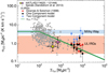 |
Fig. 9. Median CO-to-H2 conversion factor estimates as a function of the total surface density. The grey circles correspond to the αCO values based on dust emission for nearby disc galaxies (Sandstrom et al. 2013). The ULIRG data correspond to the estimates presented in Downes & Solomon (1998) and Papadopoulos et al. (2012). In the latter case, we show the αCO values reported from their “one-” and “two-component” multi-transition models. The colour bands indicate the traditional CO-to-H2 conversion factors and their uncertainties for Milky Way- and ULIRG-like systems (Bolatto et al. 2013). The green line corresponds to the αCO parametrization suggested by Bolatto et al. (2013) for galaxies with solar metallicity. For HATLAS114625, we find a lower αCO estimate than the expected value from the Bolatto et al. (2013) parametrization. In the case of HATLAS121446, we find an agreement within 1-σ uncertainty. This figure is adapted from Bolatto et al. (2013). |
However, it should be noted that molecular gas diffuse emission and its contribution to the estimated αCO values are uncertain. The CO-to-H2 conversion factor may vary significantly for this gas component depending on local environment properties (e.g. Liszt & Pety 2012). Additional observations tracing the dense molecular gas phase may help to determine whether our αCO estimations are biased towards low values or not.
We note that we have not considered the HI content in our dynamical mass approach as we expect a negligible amount of HI mass within the inner radius (R ≈ 2.3 kpc) where Mdyn was calculated. We recall that the Mdyn values calculated at these radii are the ones that strongly constrain the αCO estimates in our procedure. In local spirals, the transition from an H2-dominated ISM to an HI-dominated ISM (ΣH2 ≈ ΣHI) occurs at Σgas ∼ 12 ± 6 M⊙ pc−2 (Leroy et al. 2008). From the spatially resolved CO(1–0) observations and the adopted αCO values, we estimated ΣH2 ∼ 146 ± 93 and 127 ± 50 M⊙ pc−2 at R ≈ 2.3 kpc for the HATLAS114625 and HATLAS121446 galaxies, which supports our assumption.
Finally, we checked if our αCO estimates are reasonable given the theoretical expectation (Bolatto et al. 2013). From theories, it is expected that αCO mainly varies with the system metallicity and total surface density. However, before making any comparison, we note that HATLAS114625 and HATLAS121446 present supra-solar metallicity values in terms of the gas phase oxygen abundance (12 + log(O/H) = 8.99 and 8.72, respectively)6. We note that, from metallicities equal to or higher than the solar value, we do not expected any significant variation of αCO due to the high metal content (Bolatto et al. 2013). Thus, we simply assumed a solar metallicity when comparing our estimates with the theoretical prediction in Bolatto et al. (2013). We show this comparison in Fig. 9. We find that the reported median CO-to-H2 values are somewhat lower than the theoretical expectation but still consistent within the scatter. Our αCO estimates are, therefore, reasonable given the measured 12 + log(O/H) and ΣTot values for both starbursts.
5. Conclusions
We present new ALMA Cycle-3 and VLT-SINFONI observations tracing the CO(1–0) and Paα emission lines from three starburst galaxies at z ∼ 0.12−0.18 taken from the VALES survey. The ALMA observations were designed to deliver spatially resolved observations of the molecular gas content at  , that is, approximately the resolution of the seeing-limited SINFONI observations (
 ). Combining near-IR and sub-mm observations, we study the ionized and molecular gas dynamics at ∼kpc-scales.
One target, HATLAS090750, presents highly asymmetric morpho-kinematics, suggesting an ongoing merger. From its SINFONI observation, we also detected fainter ro-vibrational warm molecular gas transitions along with an ionized helium line in its central galactic zone. The H2 emission lines were used to determine a warm molecular gas temperature of ∼1700 ± 500 K (Fig. C.1), which was probably produced by supernova remnant (SNR) shocks. However, we could not discard non-thermal gas excitation sources due to the lack of H2 emission line intensity measurements with different vibrational energy levels (e.g. Davies et al. 2003).
The other two starburst galaxies, HATLAS114625 and HATLAS121446, show disc-like morpho-kinematics, with rotation as the dominant component supporting self-gravity (Vrot/σv ∼ 7−8). For both systems, we model the CO and Paα galactic dynamics, and we aid the kinematic modelling by using K-band photometric models to constrain the inclination angle parameter. From those analyses, we find that the CO and Paα dynamics present a good agreement in both galaxies (Fig. 3), as suggested by similar kinematic position angles (ΔPA ∼ 4 deg) and emission line spatial extensions (R1/2, Paα/R1/2, CO ∼ 1). Our observations suggest that the ionized and molecular gas components display roughly the same galaxy morpho-kinematics.
We estimate the total mass budget for both the HATLAS114625 and HATLAS121446 galaxies by calculating the dynamical masses assuming the thin- and thick-disc hydrostatic equilibrium approximations (Burkert et al. 2010) along with two different surface density profile models. We obtain αCO values in the range of 0.7−1.2 M⊙ (K km s−1 pc2)−1 for both galaxies (Fig. 5), that is, similar values to those reported for ULIRGs (Downes & Solomon 1998). These values do not depend strongly on the hydrostatic equilibrium and total surface density assumptions. Our conversion factor estimates are somewhat lower but still consistent with the  trend suggested from theoretical expectations (Fig. 9, Bolatto et al. 2013).
By adopting the dynamically based αCO values, we obtain molecular gas fractions of the order of ∼0.1 for both starbursts, far below our initial expectations and consistent with values measured in local SFGs. Therefore, the sources are not gas-rich, as initially thought, highlighting the difficulties in estimating molecular gas masses due to the uncertainty of the CO-to-H2 conversion factor.
We find that the HATLAS114625 and HATLAS121446 molecular gas velocity dispersion values are reasonably represented by a  trend, where Σtot is the total galaxy surface density (Fig. 6). This suggests that the molecular gas velocity dispersion values are consistent with being set by the galaxy self-gravity to maintain the vertical pressure balance.
We study the star-formation activity traced at ∼kpc-scales in the HATLAS114625 and HATLAS121446 starbursts. Both galaxies exhibit τdep values in the range of ∼0.1−1 Gyr (Fig. 7), that is, values consistent with the reported estimates for ULIRGs (τdep ∼ 0.1 Gyr). However, both systems present ΣH2 values that are comparable to those seen in local star-forming disc galaxies (Leroy et al. 2013). This suggests that the decrease in τdep (or enhancement of the SFE) is also produced by additional physical processes that may not only be related to high-ΣH2 environments.
To further explore this, we study the correlation between ΣSFR and the gravitational pressure Pgrav. HATLAS114625 and HATLAS121446 fill the gap between normal galaxies and ULIRG systems in terms of pressure set by self-gravity. We find a linear relation in the log-log space, log10(ΣSFR) = N × log10(Pgrav/P0), where N = 0.78 ± 0.01 and log10(P0/kB[cm−3 K]) = 5.38 ± 0.04 (Fig. 8). This is in agreement with the trend reported for local galaxies in Sun et al. (2020), suggesting that, in these z ∼ 0.12−0.17 dusty starburst galaxies, the star-formation activity can be a consequence of the ISM pressure balance.
For a typical H II region with a temperature of 104 K, we expect a Paα thermal broadening of ∼20 km s−1. For the molecular gas ISM phase with a temperature of ≲200 K, we expect thermally broadened CO line widths ≲0.5 km s−1.
The Hα flux estimates are taken from the GAMA survey DR3 (see Table A.1).
Defined as the region within three times the synthesized beam size from the best-fit galactic dynamical centre (see Fig. 3).
Compared to Eq. (6), ΣTot is replaced by [ΣH2 + s Σ⋆] and γ = 0.
We base our metallicity estimates on the Pettini & Pagel (2004) calibration scale and the [N II] and Hα line intensities reported in Table A.1. We also adopt a solar abundance of 12 + log(O/H) = 8.69 (Asplund et al. 2009).
Acknowledgments
We thank the anonymous referee for her/his careful reading of our manuscript as well as helpful comments and suggestions. This work was supported by the National Science Foundation of China (11421303, 11721303, 11890693, 11991052) and the National Key R&D Program of China (2016YFA0400702, 2016YFA0400703). We acknowledge Prof. Fisher for kindly sharing his data. J. M. and A. E. acknowledge support from CONICYT project Basal AFB-170002 and Proyecto Regular FONDECYT (grant 1181663). E. I. acknowledges partial support from FONDECYT through grant N° 1171710. N. G. acknowledges financial support from ICM Núcleo Milenio de Formación Planetaria, NPF and grant support from project CONICYT-PFCHA/Doctorado Nacional/2017 folio 21170650. C. C. is supported by the National Natural Science Foundation of China, No. 11803044, 11933003, 11673028 and by the National Key R&D Program of China grant 2017YFA0402704. M. J. M. acknowledges the support of the National Science Centre, Poland through the SONATA BIS grant 2018/30/E/ST9/00208. This work is sponsored (in part) by the Chinese Academy of Sciences (CAS), through a grant to the CAS South America Center for Astronomy (CASSACA). This paper makes use of the following ALMA data: ADS/JAO.ALMA#2015.1.01012.S. ALMA is a partnership of ESO (representing its member states), NSF (USA) and NINS (Japan), together with NRC (Canada), MOST and ASIAA (Taiwan), and KASI (Republic of Korea), in cooperation with the Republic of Chile. The Joint ALMA Observatory is operated by ESO, AUI/NRAO and NAOJ. This work is also based on observations collected at the European Organization for Astronomical Research in the Southern Hemisphere under ESO programme ID 099.B-0479(A).
References
- Asplund, M., Grevesse, N., Sauval, A. J., & Scott, P. 2009, ARA&A, 47, 481 [NASA ADS] [CrossRef] [Google Scholar]
- Baldry, I. K., Liske, J., Brown, M. J. I., et al. 2018, MNRAS, 474, 3875 [NASA ADS] [CrossRef] [Google Scholar]
- Baldwin, J. A., Phillips, M. M., & Terlevich, R. 1981, PASP, 93, 5 [NASA ADS] [CrossRef] [EDP Sciences] [Google Scholar]
- Bayo, A., Rodrigo, C., Barrado Y Navascués, D., et al. 2008, A&A, 492, 277 [NASA ADS] [CrossRef] [EDP Sciences] [Google Scholar]
- Bedregal, A. G., Colina, L., Alonso-Herrero, A., & Arribas, S. 2009, ApJ, 698, 1852 [NASA ADS] [CrossRef] [Google Scholar]
- Benincasa, S. M., Wadsley, J., Couchman, H. M. P., & Keller, B. W. 2016, MNRAS, 462, 3053 [CrossRef] [Google Scholar]
- Benjamin, R. A., Skillman, E. D., & Smits, D. P. 1999, ApJ, 514, 307 [NASA ADS] [CrossRef] [Google Scholar]
- Bigiel, F., Leroy, A., Walter, F., et al. 2008, AJ, 136, 2846 [NASA ADS] [CrossRef] [Google Scholar]
- Binney, J., & Tremaine, S. 2008, Galactic Dynamics: Second Edition (Princeton: Princeton University Press) [Google Scholar]
- Black, J. H., & van Dishoeck, E. F. 1987, ApJ, 322, 412 [NASA ADS] [CrossRef] [Google Scholar]
- Bolatto, A. D., Wolfire, M., & Leroy, A. K. 2013, ARA&A, 51, 207 [Google Scholar]
- Bolatto, A. D., Wong, T., Utomo, D., et al. 2017, ApJ, 846, 159 [NASA ADS] [CrossRef] [Google Scholar]
- Bothwell, M. S., Smail, I., Chapman, S. C., et al. 2013, MNRAS, 429, 3047 [Google Scholar]
- Bournaud, F., Elmegreen, B. G., & Elmegreen, D. M. 2007, ApJ, 670, 237 [Google Scholar]
- Bournaud, F., Elmegreen, B. G., Teyssier, R., Block, D. L., & Puerari, I. 2010, MNRAS, 409, 1088 [NASA ADS] [CrossRef] [Google Scholar]
- Brand, P. W. J. L., Toner, M. P., Geballe, T. R., & Webster, A. S. 1989, MNRAS, 237, 1009 [CrossRef] [Google Scholar]
- Bryant, J. J., Owers, M. S., Robotham, A. S. G., et al. 2015, MNRAS, 447, 2857 [NASA ADS] [CrossRef] [Google Scholar]
- Burkert, A., Genzel, R., Bouché, N., et al. 2010, ApJ, 725, 2324 [NASA ADS] [CrossRef] [Google Scholar]
- Burkert, A., Förster Schreiber, N. M., Genzel, R., et al. 2016, ApJ, 826, 214 [NASA ADS] [CrossRef] [Google Scholar]
- Calabrò, A., Daddi, E., Cassata, P., et al. 2018, ApJ, 862, L22 [NASA ADS] [CrossRef] [Google Scholar]
- Calistro Rivera, G., Hodge, J. A., Smail, I., et al. 2018, ApJ, 863, 56 [NASA ADS] [CrossRef] [Google Scholar]
- Calzetti, D., Armus, L., Bohlin, R. C., et al. 2000, ApJ, 533, 682 [NASA ADS] [CrossRef] [Google Scholar]
- Carilli, C. L., & Walter, F. 2013, ARA&A, 51, 105 [NASA ADS] [CrossRef] [EDP Sciences] [Google Scholar]
- Chabrier, G. 2003, PASP, 115, 763 [Google Scholar]
- Cheng, C., Ibar, E., Hughes, T. M., et al. 2018, MNRAS, 475, 248 [CrossRef] [Google Scholar]
- Cluver, M. E., Jarrett, T. H., Hopkins, A. M., et al. 2014, ApJ, 782, 90 [NASA ADS] [CrossRef] [Google Scholar]
- Colina, L., Piqueras López, J., Arribas, S., et al. 2015, A&A, 578, A48 [NASA ADS] [CrossRef] [EDP Sciences] [Google Scholar]
- Combes, F., Boquien, M., Kramer, C., et al. 2012, A&A, 539, A67 [NASA ADS] [CrossRef] [EDP Sciences] [Google Scholar]
- Courteau, S. 1997, AJ, 114, 2402 [NASA ADS] [CrossRef] [Google Scholar]
- Crowther, P. A. 2007, ARA&A, 45, 177 [NASA ADS] [CrossRef] [Google Scholar]
- Da Cunha, E., Charlot, S., & Elbaz, D. 2008, MNRAS, 388, 1595 [NASA ADS] [CrossRef] [Google Scholar]
- Daddi, E., Bournaud, F., Walter, F., et al. 2010, ApJ, 713, 686 [NASA ADS] [CrossRef] [Google Scholar]
- Davies, R. I., Sternberg, A., Lehnert, M., & Tacconi-Garman, L. E. 2003, ApJ, 597, 907 [NASA ADS] [CrossRef] [Google Scholar]
- de Blok, W. J. G., Walter, F., Brinks, E., et al. 2008, AJ, 136, 2648 [NASA ADS] [CrossRef] [Google Scholar]
- Dekel, A., Sari, R., & Ceverino, D. 2009, ApJ, 703, 785 [Google Scholar]
- Downes, D., & Solomon, P. M. 1998, ApJ, 507, 615 [NASA ADS] [CrossRef] [Google Scholar]
- Draine, B. T., & Woods, D. T. 1990, ApJ, 363, 464 [NASA ADS] [CrossRef] [Google Scholar]
- Driver, S. P., Wright, A. H., Andrews, S. K., et al. 2016, MNRAS, 455, 3911 [NASA ADS] [CrossRef] [Google Scholar]
- Eales, S., Dunne, L., Clements, D., et al. 2010, PASP, 122, 499 [NASA ADS] [CrossRef] [Google Scholar]
- Eisenhauer, F., Abuter, R., Bickert, K., et al. 2003, in Instrument Design and Performance for Optical/Infrared Ground-based Telescopes, eds. M. Iye, & A. F. M. Moorwood, Proc. SPIE, 4841, 1548 [NASA ADS] [CrossRef] [Google Scholar]
- Elmegreen, B. G. 1989, ApJ, 338, 178 [NASA ADS] [CrossRef] [Google Scholar]
- Elmegreen, B. G., & Scalo, J. 2004, ARA&A, 42, 211 [NASA ADS] [CrossRef] [Google Scholar]
- Epinat, B., Tasca, L., Amram, P., et al. 2012, A&A, 539, A92 [NASA ADS] [CrossRef] [EDP Sciences] [Google Scholar]
- Espada, D., Martin, S., Verley, S., et al. 2018, ApJ, 866, 77 [CrossRef] [Google Scholar]
- Faucher-Giguère, C.-A., Quataert, E., & Hopkins, P. F. 2013, MNRAS, 433, 1970 [NASA ADS] [CrossRef] [Google Scholar]
- Fazeli, N., Busch, G., Valencia-S., M., et al. 2019, A&A, 622, A128 [NASA ADS] [CrossRef] [EDP Sciences] [Google Scholar]
- Fisher, D. B., Bolatto, A. D., White, H., et al. 2019, ApJ, 870, 46 [CrossRef] [Google Scholar]
- Foreman-Mackey, D., Hogg, D. W., Lang, D., & Goodman, J. 2013, PASP, 125, 306 [CrossRef] [Google Scholar]
- Freeman, K. C. 1970, ApJ, 160, 811 [Google Scholar]
- Geach, J. E., Sobral, D., Hickox, R. C., et al. 2012, MNRAS, 426, 679 [NASA ADS] [CrossRef] [Google Scholar]
- Gentry, E. S., Krumholz, M. R., Dekel, A., & Madau, P. 2017, MNRAS, 465, 2471 [CrossRef] [Google Scholar]
- Gentry, E. S., Krumholz, M. R., Madau, P., & Lupi, A. 2019, MNRAS, 483, 3647 [CrossRef] [Google Scholar]
- Genzel, R., Tacconi, L. J., Gracia-Carpio, J., et al. 2010, MNRAS, 407, 2091 [NASA ADS] [CrossRef] [Google Scholar]
- Genzel, R., Tacconi, L. J., Lutz, D., et al. 2015, ApJ, 800, 20 [NASA ADS] [CrossRef] [Google Scholar]
- Goldsmith, P. F., Heyer, M., Narayanan, G., et al. 2008, ApJ, 680, 428 [NASA ADS] [CrossRef] [Google Scholar]
- Green, A. W., Glazebrook, K., McGregor, P. J., et al. 2014, MNRAS, 437, 1070 [NASA ADS] [CrossRef] [Google Scholar]
- Hayward, C. C., & Hopkins, P. F. 2017, MNRAS, 465, 1682 [Google Scholar]
- Herrera-Camus, R., Bolatto, A., Wolfire, M., et al. 2017, ApJ, 835, 201 [NASA ADS] [CrossRef] [Google Scholar]
- Holmberg, E. 1958, Meddelanden fran Lunds Astronomiska Observatorium Serie II, 136, 1 [Google Scholar]
- Ibar, E., Lara-López, M. A., Herrera-Camus, R., et al. 2015, MNRAS, 449, 2498 [NASA ADS] [CrossRef] [Google Scholar]
- Kauffmann, G., Heckman, T. M., Tremonti, C., et al. 2003, MNRAS, 346, 1055 [Google Scholar]
- Kausch, W., Noll, S., Smette, A., et al. 2015, A&A, 576, A78 [NASA ADS] [CrossRef] [EDP Sciences] [Google Scholar]
- Kelvin, L. S., Driver, S. P., Robotham, A. S. G., et al. 2012, MNRAS, 421, 1007 [NASA ADS] [CrossRef] [Google Scholar]
- Kennicutt, R. C., Jr. 1998a, ApJ, 498, 541 [NASA ADS] [CrossRef] [Google Scholar]
- Kennicutt, R. C., Jr. 1998b, ARA&A, 36, 189 [Google Scholar]
- Kereš, D., Katz, N., Weinberg, D. H., & Davé, R. 2005, MNRAS, 363, 2 [Google Scholar]
- Kewley, L. J., Dopita, M. A., Sutherland, R. S., Heisler, C. A., & Trevena, J. 2001, ApJ, 556, 121 [Google Scholar]
- Kim, C.-G., & Ostriker, E. C. 2015, ApJ, 802, 99 [NASA ADS] [CrossRef] [Google Scholar]
- Kim, C.-G., Kim, W.-T., & Ostriker, E. C. 2011, ApJ, 743, 25 [NASA ADS] [CrossRef] [Google Scholar]
- Kim, C.-G., Ostriker, E. C., & Kim, W.-T. 2013, ApJ, 776, 1 [NASA ADS] [CrossRef] [Google Scholar]
- Kim, C.-G., Ostriker, E. C., & Raileanu, R. 2017, ApJ, 834, 25 [NASA ADS] [CrossRef] [Google Scholar]
- Kronberger, T., Kapferer, W., Schindler, S., & Ziegler, B. L. 2007, A&A, 473, 761 [Google Scholar]
- Krumholz, M. R., & Burkhart, B. 2016, MNRAS, 458, 1671 [NASA ADS] [CrossRef] [Google Scholar]
- Krumholz, M. R., Burkhart, B., Forbes, J. C., & Crocker, R. M. 2018, MNRAS, 477, 2716 [NASA ADS] [CrossRef] [Google Scholar]
- Lang, P., Förster Schreiber, N. M., Genzel, R., et al. 2017, ApJ, 840, 92 [NASA ADS] [CrossRef] [Google Scholar]
- Larkin, J. E., Armus, L., Knop, R. A., Soifer, B. T., & Matthews, K. 1998, ApJS, 114, 59 [NASA ADS] [CrossRef] [Google Scholar]
- Lefever, K., Puls, J., Morel, T., et al. 2010, A&A, 515, A74 [NASA ADS] [CrossRef] [EDP Sciences] [Google Scholar]
- Leroy, A. K., Walter, F., Brinks, E., et al. 2008, AJ, 136, 2782 [Google Scholar]
- Leroy, A. K., Walter, F., Bigiel, F., et al. 2009, AJ, 137, 4670 [NASA ADS] [CrossRef] [Google Scholar]
- Leroy, A. K., Walter, F., Sandstrom, K., et al. 2013, AJ, 146, 19 [NASA ADS] [CrossRef] [Google Scholar]
- Levy, R. C., Bolatto, A. D., Teuben, P., et al. 2018, ApJ, 860, 92 [NASA ADS] [CrossRef] [Google Scholar]
- Liszt, H. S., & Pety, J. 2012, A&A, 541, A58 [NASA ADS] [CrossRef] [EDP Sciences] [Google Scholar]
- Madau, P., & Dickinson, M. 2014, ARA&A, 52, 415 [NASA ADS] [CrossRef] [Google Scholar]
- Madau, P., Ferguson, H. C., Dickinson, M. E., et al. 1996, MNRAS, 283, 1388 [NASA ADS] [CrossRef] [Google Scholar]
- Martizzi, D., Faucher-Giguère, C.-A., & Quataert, E. 2015, MNRAS, 450, 504 [NASA ADS] [CrossRef] [Google Scholar]
- Mateos, S., Alonso-Herrero, A., Carrera, F. J., et al. 2012, MNRAS, 426, 3271 [NASA ADS] [CrossRef] [Google Scholar]
- Michałowski, M. J., Hayward, C. C., Dunlop, J. S., et al. 2014, A&A, 571, A75 [NASA ADS] [CrossRef] [EDP Sciences] [Google Scholar]
- Molina, J., Ibar, E., Villanueva, V., et al. 2019a, MNRAS, 482, 1499 [CrossRef] [Google Scholar]
- Molina, J., Ibar, E., Smail, I., et al. 2019b, MNRAS, 487, 4856 [CrossRef] [Google Scholar]
- Mosenkov, A. V., Sotnikova, N. Y., Reshetnikov, V. P., Bizyaev, D. V., & Kautsch, S. J. 2015, MNRAS, 451, 2376 [NASA ADS] [CrossRef] [Google Scholar]
- Motta, V., Ibar, E., Verdugo, T., et al. 2018, ApJ, 863, L16 [NASA ADS] [CrossRef] [Google Scholar]
- Narayanan, D., Krumholz, M. R., Ostriker, E. C., & Hernquist, L. 2012, MNRAS, 421, 3127 [NASA ADS] [CrossRef] [Google Scholar]
- Newville, M., Stensitzki, T., Allen, D. B., & Ingargiola, A. 2014, https://doi.org/10.5281/zenodo.11813 [Google Scholar]
- Niemczura, E., Morel, T., & Aerts, C. 2009, A&A, 506, 213 [NASA ADS] [CrossRef] [EDP Sciences] [Google Scholar]
- Noll, S., Kausch, W., Kimeswenger, S., et al. 2014, A&A, 567, A25 [NASA ADS] [CrossRef] [EDP Sciences] [Google Scholar]
- Oliva, E., Moorwood, A. F. M., & Danziger, I. J. 1990, A&A, 240, 453 [NASA ADS] [Google Scholar]
- Osterbrock, D. E., & Ferland, G. J. 2006, Astrophysics of Gaseous Nebulae and Active Galactic Nuclei (Sausalito, CA: University Science Books) [Google Scholar]
- Ostriker, E. C., & Shetty, R. 2011, ApJ, 731, 41 [NASA ADS] [CrossRef] [Google Scholar]
- Ostriker, J. P., Choi, E., Ciotti, L., Novak, G. S., & Proga, D. 2010, ApJ, 722, 642 [NASA ADS] [CrossRef] [Google Scholar]
- Papadopoulos, P. P., & Seaquist, E. R. 1999, ApJ, 516, 114 [NASA ADS] [CrossRef] [Google Scholar]
- Papadopoulos, P. P., van der Werf, P., Xilouris, E., Isaak, K. G., & Gao, Y. 2012, ApJ, 751, 10 [NASA ADS] [CrossRef] [Google Scholar]
- Pettini, M., & Pagel, B. E. J. 2004, MNRAS, 348, L59 [NASA ADS] [CrossRef] [Google Scholar]
- Piqueras López, J., Colina, L., Arribas, S., Alonso-Herrero, A., & Bedregal, A. G. 2012, A&A, 546, A64 [NASA ADS] [CrossRef] [EDP Sciences] [Google Scholar]
- Riffel, R., Rodríguez-Ardila, A., Aleman, I., et al. 2013, MNRAS, 430, 2002 [NASA ADS] [CrossRef] [Google Scholar]
- Saintonge, A., Catinella, B., Tacconi, L. J., et al. 2017, ApJS, 233, 22 [Google Scholar]
- Sánchez, S. F., Kennicutt, R. C., Gil de Paz, A., et al. 2012, A&A, 538, A8 [NASA ADS] [CrossRef] [EDP Sciences] [Google Scholar]
- Sandstrom, K. M., Leroy, A. K., Walter, F., et al. 2013, ApJ, 777, 5 [NASA ADS] [CrossRef] [Google Scholar]
- Schawinski, K., Thomas, D., Sarzi, M., et al. 2007, MNRAS, 382, 1415 [NASA ADS] [CrossRef] [Google Scholar]
- Schinnerer, E., Weiß, A., Aalto, S., & Scoville, N. Z. 2010, ApJ, 719, 1588 [NASA ADS] [CrossRef] [Google Scholar]
- Schruba, A., Kruijssen, J. M. D., & Leroy, A. K. 2019, ApJ, 883, 2 [CrossRef] [Google Scholar]
- Sérsic, J. L. 1963, Boletin de la Asociacion Argentina de Astronomia La Plata Argentina, 6, 41 [Google Scholar]
- Sharma, P., Roy, A., Nath, B. B., & Shchekinov, Y. 2014, MNRAS, 443, 3463 [NASA ADS] [CrossRef] [Google Scholar]
- Shetty, R., & Ostriker, E. C. 2012, ApJ, 754, 2 [NASA ADS] [CrossRef] [Google Scholar]
- Shi, Y., Helou, G., Yan, L., et al. 2011, ApJ, 733, 87 [NASA ADS] [CrossRef] [Google Scholar]
- Solomon, P. M., & Vanden Bout, P. A. 2005, ARA&A, 43, 677 [NASA ADS] [CrossRef] [Google Scholar]
- Solomon, P. M., Rivolo, A. R., Barrett, J., & Yahil, A. 1987, ApJ, 319, 730 [NASA ADS] [CrossRef] [Google Scholar]
- Spitzer, L., Jr. 1942, ApJ, 95, 329 [NASA ADS] [CrossRef] [Google Scholar]
- Spring, E. F., & Michałowski, M. J. 2017, MNRAS, 471, L101 [NASA ADS] [CrossRef] [Google Scholar]
- Stern, D., Assef, R. J., Benford, D. J., et al. 2012, ApJ, 753, 30 [NASA ADS] [CrossRef] [Google Scholar]
- Sternberg, A. 1989, ApJ, 347, 863 [NASA ADS] [CrossRef] [Google Scholar]
- Stott, J. P., Swinbank, A. M., Johnson, H. L., et al. 2016, MNRAS, 457, 1888 [NASA ADS] [CrossRef] [Google Scholar]
- Sun, J., Leroy, A. K., Ostriker, E. C., et al. 2020, ApJ, 892, 148 [CrossRef] [Google Scholar]
- Swinbank, A. M., Sobral, D., Smail, I., et al. 2012, MNRAS, 426, 935 [NASA ADS] [CrossRef] [Google Scholar]
- Tacconi, L. J., Genzel, R., Neri, R., et al. 2010, Nature, 463, 781 [Google Scholar]
- Tacconi, L. J., Genzel, R., Saintonge, A., et al. 2018, ApJ, 853, 179 [NASA ADS] [CrossRef] [Google Scholar]
- Thompson, T. A., Quataert, E., & Murray, N. 2005, ApJ, 630, 167 [NASA ADS] [CrossRef] [Google Scholar]
- Thornton, K., Gaudlitz, M., Janka, H. T., & Steinmetz, M. 1998, ApJ, 500, 95 [NASA ADS] [CrossRef] [Google Scholar]
- U, V., Medling, A. M., Inami, H., et al. 2019, ApJ, 871, 166 [CrossRef] [Google Scholar]
- Varidel, M. R., Croom, S. M., Lewis, G. F., et al. 2020, MNRAS, 495, 2265 [CrossRef] [Google Scholar]
- Villanueva, V., Ibar, E., Hughes, T. M., et al. 2017, MNRAS, 470, 3775 [NASA ADS] [CrossRef] [Google Scholar]
- Walter, F., Brinks, E., de Blok, W. J. G., et al. 2008, AJ, 136, 2563 [Google Scholar]
- Whitaker, K. E., van Dokkum, P. G., Brammer, G., & Franx, M. 2012, ApJ, 754, L29 [NASA ADS] [CrossRef] [Google Scholar]
- Wilson, C. D., Elmegreen, B. G., Bemis, A., & Brunetti, N. 2019, ApJ, 882, 5 [NASA ADS] [CrossRef] [Google Scholar]
- Wolniewicz, L., Simbotin, I., & Dalgarno, A. 1998, ApJS, 115, 293 [NASA ADS] [CrossRef] [Google Scholar]
- Wong, T., & Blitz, L. 2002, ApJ, 569, 157 [NASA ADS] [CrossRef] [Google Scholar]
- Wright, E. L., Eisenhardt, P. R. M., Mainzer, A. K., et al. 2010, AJ, 140, 1868 [Google Scholar]
- Zhou, L., Federrath, C., Yuan, T., et al. 2017, MNRAS, 470, 4573 [CrossRef] [Google Scholar]
Appendix A: Emission line and WISE colour fluxes
Summary of the emission line and WISE colour fluxes used in this work and taken from the GAMA DR3 (Baldry et al. 2018).
Appendix B: Experimental observation results
We performed an on-source experimental jittering pattern to optimize the S/N of the Paα emission line for HATLAS090750. In this experimental observation, the pointing was kept fixed at the galaxy location. Hence, an OOOO jitter sequence was used. As we do not observe the sky during this observation, the emission and telluric absorption bandpass lines need to be subtracted using sky models. Specifically, we used the SKYCOR and MOLECFIT pipelines. This implies that the performance of this experimental observation is mainly limited by the accuracy of the sky emission modelling and the ability to detect the line emission (S/N ≳ 15; Godoy et al., in prep.).
Figure 2 clearly shows that we were able to detect the targeted emission line (Paα) for this galaxy (S/N = 80). We were also able to observe many other fainter near-IR emission lines (Table C.1) that allowed us to study the conditions of the host molecular gas ISM (Appendix C). Faint tidal features were also detected for this system, demonstrating the ability of this observation to recover the galaxy spatial distribution when compared, for example, to the CO(1–0) observation (Fig. 3). Thus, this experimental observation delivered more information than initially expected and allowed us to study HATLAS090750 in great detail.
Even though we have not provided a reliable flux calibration for HATLAS090750, we note that this was because we were unable to accurately model the telluric standard star (HD 56006) observation. For most of the observed telluric standards, the effective temperature agrees well in the literature with very low dispersion, allowing an appropriate calibration using a black body. However, HD 56006 has very uncertain stellar parameters (e.g. Niemczura et al. 2009; Lefever et al. 2010), making a reliable calibration impossible even in the case when more sophisticated approaches were attempted. We highlight that this problem is only related to this standard star observation. If a flux standard star had been observed, then the OOOO observation flux calibration would have been straightforward. Thus, we conclude that our observational experiment was a success. We recommend adopting this experimental OOOO observational setup when the expected line emission S/N is ∼15 or greater.
Appendix C: Near-IR emission lines
Near-IR emission lines are useful for determining the excitation mechanism of the gaseous line-emitting ISM. Similar to the well-established optical diagnostic diagrams (e.g. the BPT diagram), the ratio between star-formation line tracers (e.g. Paα, Paβ) and shock tracers, such as ro-vibrational molecular hydrogen emission lines (e.g. H2(1–0)S(1)λ2.122 μm) or forbidden iron lines ([Fe II]λ1.64 μm), can be used to determine the dominant excitation mechanism (e.g. Larkin et al. 1998; Riffel et al. 2013; Fazeli et al. 2019).
From the central brightest pixels from our SINFONI K-band observations, we detected more near-IR emission lines than only Paα (Fig. 2). By considering a circular aperture with a radius equal to the PSF FWHM and centred at the galaxy Paα luminosity peak, we measured several other emission lines fluxes (see Table C.1). These values were estimated by fitting a Gaussian function to each emission line in the spatially collapsed spectrum, and the 1-σ uncertainties were derived by bootstrapping via Monte Carlo simulations the flux-density errors. These ratio values were corrected by assuming a Calzetti et al. (2000) attenuation law (APaα = 0.145 AV, ABrδ = 0.132 AV, AHeI = 0.113 AV, AH2(1−0)S(3) = 0.130 AV, AH2(1−0)S(2) = 0.117 AV, AH2(1−0)S(1) = 0.103 AV). We note that this correction is determined by the shape of the assumed attenuation law.
Spatially integrated Brδλ1.944 μm, ro-vibrational H2(1–0)S(3)λ1.957 μm, H2(1–0)S(2)λ2.033 μm, H2(1–0)S(1)λ2.122 μm, and HeIλ2.058 μm fluxes relative to the Paα emission line flux.
We could only apply the near-IR emission line analysis to the HATLAS090750 galaxy as we lack enough H2 emission line flux measurements for the other two systems. For this galaxy, we used the Paα flux intensity to differentiate between the possible excitation mechanisms. The other option, the use of the Brγ emission line, was impeded given that this emission line is redshifted out of the SINFONI K-band wavelength range. This means that the H2(1–0)S(1)/Brγ ≈ 0.8 ratio that differentiates star-forming regions from SNR shocks and compact AGN activity is translated to H2(1–0)S(1)/Paα ≈ 0.07 (assuming a Brγ-to-Paα intrinsic ratio of 12.19 (Case B recombination, Osterbrock & Ferland 2006)).
HATLAS090750 shows a central H2(1–0)S(1)/Paα ratio consistent with the median value measured for local LIRGs (z ≲ 0.02; Colina et al. 2015). This ratio suggests that there is no clear dominant gas excitation mechanism in this galaxy; it is likely a combined effect of UV photons produced by young O-B stars, SNR shocks, and weak AGN activity (Colina et al. 2015).
The detection of HeIλ2.058 μm suggests that we are witnessing a young central starburst that was probably induced by the ongoing merger. Unfortunately, we cannot constrain the ISM physical properties from this emission line as we lack the detection of additional HeI emission lines (e.g. Benjamin et al. 1999).
We further characterize the HATLAS090750 ISM warm molecular gas phase by using the logNν, J/gν, J − E excitation diagram (Davies et al. 2003). In this diagram, Nν, J is the molecular column density, gν, J is the statistical weight, and E is the upper energy level of the ro-vibrational transition. From the H2 emission line fluxes fν, J, the column densities in the upper ro-vibrational levels are computed as:
 (C.1)
(C.1)
where Ω is the spectrum extraction aperture size, Aul is the Einstein coefficient computed by Wolniewicz et al. (1998), and λ/hc is the photon energy. Additionally, the Nν, J/gν, J ratios need to be normalized to a specific population distribution value Nν0, J0/gν0, J0 given from a determined H2 transition. We normalized them to the inferred value from the H2(1–0)S(3) emission line transition (e.g. Bedregal et al. 2009). We note that if the warm molecular gas phase is in local thermodynamic equilibrium (LTE), then the data are well described by a simple linear function that represents a Boltzmann distribution characterized by a single excitation temperature.
In Fig. C.1, we show the excitation diagram. As we lack H2 emission line intensity measurements with different vibrational energy levels, we can only measure rotational temperature Trot for the vibrational H2(ν = 1−0) transition. We find that the data are well fitted by a linear fit with Trot ≈ 1600 ± 400 K, suggesting that the warm H2 ISM phase in the central brightest zone of this galaxy is in LTE.
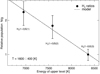 |
Fig. C.1. Gas excitation diagram for the H2 emission coming from the central part of the HATLAS090750 galaxy. The Nν, J/gν, J ratios are normalized to the value inferred from the H2(1–0)S(3) emission line transition. The population levels are well characterized by a Boltzmann distribution, suggesting that the warm H2 gas is in LTE. |
This temperature value also suggests that the warm H2 gas may be mainly heated by SNR shocks (Brand et al. 1989; Oliva et al. 1990), with perhaps some contribution from thermal X-ray heating from SNRs (Trot ≳ 2000 K, e.g. Draine & Woods 1990). Thermal UV heating is unlikely as models suggest lower temperature values (Trot ≲ 1000 K, Sternberg 1989). However, we stress that we cannot rule out non-thermal UV excitation (e.g. fluorescence; Black & van Dishoeck 1987) as we lack H2 emission line observations with different vibrational energy levels (Bedregal et al. 2009). Nevertheless, our Trot estimate is slightly higher than, but still consistent with, the average value (⟨Trot⟩∼1360 ± 390 K) reported for local (z < 0.08) LIRGs (U et al. 2019).
Appendix D: Beam-smearing effect on the rotation velocity values
Accurate rotation velocities cannot be derived towards the centres of galaxies due to beam-smearing effects. Rotation velocities tend to be underestimated due to the flux-weighted nature of the data convolution with the PSF and/or synthesized beam. Thus, a beam-smearing correction needs to be applied.
Based on our best-fit two-dimensional models, we quantified the beam-smearing effect on rotation velocities by computing the beam-smeared to intrinsic ARCTAN best-fit velocity model ratio and measured across the galaxies major kinematic axes. We show the estimation of this ratio in Fig. D.1 for the ALMA and VLT-SINFONI observations of the HATLAS114625 and HATLAS121446 galaxies. We find that a moderate beam-smearing correction (≲10%) needs to be applied to the rotation velocity values measured at a galactocentric radius longer than 1.5× projected synthesized beam or PSF FWHM. At smaller radii, the beam-smearing effect tends to increase dramatically.
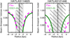 |
Fig. D.1. Beam-smearing effect on the recovered rotation velocity values across the major kinematic axis for HATLAS114625 (left) and HATLAS121446 (right) galaxies. We mask the values at R ≤ 0.5× synthesized beam or PSF FWHM due to the highly uncertain estimates and to improve visualization. The colour codes are the same as in Fig. 4. At a radius R ≳ 1.5× synthesized beam or PSF FWHM from the dynamical centre, we estimate that a moderate correction (≲10%) needs to be applied to the observed rotation velocity values. |
Appendix E: SINFONI K-band continuum maps
In Fig. E.1, we show the continuum maps used to calculate the pixel-by-pixel Σ⋆ values. These maps are scaled to the respective galaxy M⋆ value, that is, by assuming a constant mass-to-light ratio across the galactic disc.
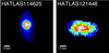 |
Fig. E.1. SINFONI K-band continuum maps for HATLAS114625 (left) and HATLAS121446 (right) targets. |
Appendix F: Full αCO and dark matter PDFs
Our dynamical mass approach is limited by the degeneracy between αCO and the dark matter fraction fDM variables. Due to our assumption of a constant αCO value across the galactic disc, the dynamical mass value estimated at the innermost galactocentric radius limits the maximum αCO value that can be obtained. At this radius, fDM is consistent with zero, but this does not necessarily hold at longer radii.
In Fig. F.1, we show the αCO and fDM(R) PDFs derived from the “thick-disc plus Sérsic” dynamical mass model, that is, the model that determines the adopted median αCO value in our work. There is no major difference between the αCO PDF obtained from this model and those derived from other dynamical models, as the broad αCO PDF shapes prove (Fig. 5).
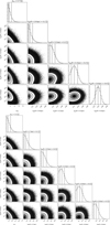 |
Fig. F.1. Corner plot for αCO and fDM(R) variables for the HATLAS114625 (top) and HATLAS121446 (bottom) starbursts. |
The HATLAS114625 galaxy shows a higher increase in fDM as a function of galactocentric radius compared to HATLAS121446, suggesting that baryonic matter is distributed more compactly in the former system. This is consistent with the reported K-band Sérsic index value (Table 3) and the steeper velocity gradient that is seen in HATLAS114625 (Fig. 4).
All Tables
K-band surface brightness Sérsic best-fit model parameters taken from the GAMA-DR3 for our sample (Kelvin et al. 2012).
CO-to-H2 conversion factor, molecular gas masses, and gas fractions for HATLAS114625 and HATLAS121446 starbursts.
Summary of the emission line and WISE colour fluxes used in this work and taken from the GAMA DR3 (Baldry et al. 2018).
Spatially integrated Brδλ1.944 μm, ro-vibrational H2(1–0)S(3)λ1.957 μm, H2(1–0)S(2)λ2.033 μm, H2(1–0)S(1)λ2.122 μm, and HeIλ2.058 μm fluxes relative to the Paα emission line flux.
All Figures
|
Fig. 1. Characterization of the three galaxies presented in this work in terms of stellar mass, SFRs, and AGN activity. Left: SFR–M⋆ plane. The solid and dashed lines represent the main-sequence (MS) parametrization suggested by Whitaker et al. (2012) and the 4 × SFR(MS) starburst threshold, respectively. Middle: BPT-diagram (Baldwin et al. 1981). The dashed curve shows the empirical star-forming threshold (Kauffmann et al. 2003), whereas the solid curve corresponds to the theoretical maximum starburst model (Kewley et al. 2001). These two lines encompass the SFGs-AGN “composite” zone. The dotted-dashed line indicates the division between AGNs and LINERs (Schawinski et al. 2007). Right: WISE mid-IR colour-colour diagram. The solid lines delimit the AGN-zone suggested by Mateos et al. (2012), whereas the dashed line represents the AGN threshold adopted by Stern et al. (2012). The WISE data 1-σ errorbars are smaller than the plotted symbol sizes. The GAMA data are taken from their data-release 3 (GAMA-DR3; Baldry et al. 2018), encompassing galaxies at z < 0.35 (the upper redshift limit for the VALES survey) and with 5-σ or higher flux estimates. These three panels indicate that the three galaxies presented in this work can be classified as starbursts, with one target (HATLAS114625−014511) likely to be classified as an obscured AGN host galaxy. |
| In the text | |
|
Fig. 2. Spatially integrated rest-frame spectra around the emission lines of interest. The bottom and top x-axes show the rest-frame wavelength and frequency ranges for the Paα and CO(1–0) emission lines, respectively. For each galaxy, the solid green curve shows the CO(1–0) spectrum convoluted by the SINFONI LSF. From HATLAS090750, we also detect the Brδ, H2(1–0)S(3), H2(1–0)S(2), H2(1–0)S(1), and He I near-IR emission lines using as an aperture an encircled zone given by the PSF FWHM and centred at the Paα luminosity peak. In the case of the HATLAS114625 galaxy observation, we also detect the H2(1–0)S(3) emission. These detections are shown in the sub-plots (blue-shaded area) in each panel (see also Appendix C). The CO(1–0) and Paα emission lines are clearly detected. |
| In the text | |
|
Fig. 3. K-band, intensity, velocity, velocity dispersion, and residual maps (first to fifth columns) for HATLAS090750 (top), HATLAS114625 (middle), and HATLAS121446 (bottom). For each galaxy, from the second column to the last column, we show the Paα and CO(1–0) two-dimensional maps, one above the other, respectively. The spatial scale for each observation is shown in each map. The K-band map has the CO(1–0) and Paα emissions over-plotted in green and pink contours, respectively. The CO(1–0) intensity map shows the synthesized beam size. In the velocity and velocity dispersion maps, the white cross indicates the location of the best-fitted dynamical centre. The velocity maps have the velocity contours over-plotted from their best-fit disc models, and the green- and pink-dashed lines represent the molecular and ionized gas major kinematic axes, respectively. In each velocity dispersion map, the white circumference represents the boundary of the region masked during the estimation of the global velocity dispersion value. The residual fields are constructed by subtracting the velocity disc models from the velocity maps. The rms of these residuals are given in each panel. In the case of the HATLAS090750 Paα observation, we only show the modelled central zone in the residual map. |
| In the text | |
|
Fig. 4. Rotation velocity (left) and velocity dispersion (right) profiles across the major kinematic axis for the HATLAS090750 (top), HATLAS114625 (middle), and HATLAS121446 (bottom) galaxies. The errorbars show the 1-σ uncertainties. The vertical black-dashed line represents the best-fit dynamical centre. The light grey shaded area represents the 3× synthesized beam size region centred at the best-fit molecular gas dynamical centre, whereas the dark grey dashed area represents the 3× PSF FWHM zone centred at the best-fit ionized gas dynamical centre. In the rotation velocity profile panels, the dashed-magenta and solid-green curves show the rotation curves extracted from the beam-smeared Paα and CO(1–0) two-dimensional best-fit models, respectively. In the velocity dispersion profile panels, the green- and magenta-dashed lines show the median galactic value estimated from the outskirts of the galactic disc (Table 4) for the CO(1–0) and Paα observations, respectively. We find a good agreement between the rotation curves derived from the ionized and molecular gas ISM phases in the three starbursts. |
| In the text | |
|
Fig. 5. Posterior αCO PDFs for HATLAS114625 (left) and HATLAS121446 (right) starbursts. For each galaxy, we consider four dynamical mass models encompassing different underlying surface density mass distributions and hydrostatic equilibrium approximations. We also show the cumulative probability distribution in each panel with our αCO upper limit defined as P(x < αCO, uplim) ≈ 0.997 (i.e. 3-σ) and estimated by using the thick-disc plus Sérsic dynamical mass model. The coloured arrows indicate the median αCO value for each PDF. We find median αCO estimates consistent with the ULIRG-like value for both starburst galaxies. |
| In the text | |
|
Fig. 6. Left: pixel-by-pixel molecular gas velocity dispersion estimates as a function of molecular gas surface density. For each starburst galaxy, in grey, we show the σv, CO values that may be overestimated due to beam-smearing residual effects. The errorbar in the lower-right corner indicates the typical 1-σ uncertainty, whereas the arrow represents the systematic uncertainty given by the use of our αCO upper limit instead of the adopted value. The “z ∼ 0 ULIRG” sample is taken from Wilson et al. (2019). The “z ∼ 0 SFGs” sample estimates are galactic average values measured for a sub-sample of galaxies taken from the CARMA-EDGE survey (Bolatto et al. 2017; Levy et al. 2018). The “z ∼ 1.5 SFG” data correspond to the ∼kpc-scale measurements for a main-sequence galaxy presented in Molina et al. (2019b). The solid line represents the empirical relationship suggested by Wilson et al. (2019). The dashed line shows the empirical relationship corrected by the average ΣH2/ΣTot and Vrot, CO/σv, CO ratios measured for both systems. Middle: pixel-by-pixel σv, CO values as a function of the total surface density. Right: molecular gas scale height as a function of the total gas surface density. The last two panels are colour-coded in the same way as the left panel. The vertical pressure equilibrium model gives a reasonable representation of our data. |
| In the text | |
|
Fig. 7. ΣSFR against ΣH2 for the HATLAS114625 (left) and HATLAS121446 (right) starbursts. In each panel, the errorbar in the bottom-right corner represents the typical 1-σ uncertainty. The arrow indicates the horizontal shift of the data produced if we assume the αCO, uplim value instead of the median αCO estimate to calculate ΣH2. This is also highlighted by the lightly coloured data showed in the background. The dotted lines indicate fixed τdep values. We show ∼kpc-scale spatially resolved observations of two z ∼ 0 LIRGs (orange diamonds, Espada et al. 2018) and the median trend observed for the nearby HERACLES galaxy survey (open circles, Leroy et al. 2013). The dot-dashed line represents the best fit for the HERACLES ∼kpc-scale median values. We also present spatially resolved estimates for local ULIRGs measured at ∼350−650 pc scales (Wilson et al. 2019). In solid and dashed lines, we show the double and single power-law best fits reported by Wilson et al. (2019) for the ULIRG data, respectively. Independent of the αCO value assumed, we find lower τdep values than those measured from local normal SFGs. |
| In the text | |
|
Fig. 8. ΣSFR against the ISM pressure set by self-gravity. The PHANGS data correspond to the manually convolved kpc-scale measurements reported by Sun et al. (2020) for 28 nearby galaxies. The ULIRG data correspond to the values measured at ∼350−650 pc scales by Wilson et al. (2019). The DYNAMO data are based on galactic ionized gas velocity dispersion measurements along with spatially unresolved molecular gas observations (Fisher et al. 2019). We also present the ∼kpc-scale values measured for a typical SFG at z ∼ 1.5 (SHiZELS-19; Molina et al. 2019b). The dashed line corresponds to the best fit presented by Fisher et al. (2019) for the DYNAMO and THINGS data, while the solid black line corresponds to the best fit given by Sun et al. (2020) to the PHANGS data. The dot-dashed line corresponds to the parametrization given by Kim et al. (2013) for their set of hydrodynamical simulations. The solid red line represents our best fit. The starburst and ULIRG data are consistent with the trend reported from the nearby galaxies. The z ∼ 1.5 SFG data are in clear offset. |
| In the text | |
|
Fig. 9. Median CO-to-H2 conversion factor estimates as a function of the total surface density. The grey circles correspond to the αCO values based on dust emission for nearby disc galaxies (Sandstrom et al. 2013). The ULIRG data correspond to the estimates presented in Downes & Solomon (1998) and Papadopoulos et al. (2012). In the latter case, we show the αCO values reported from their “one-” and “two-component” multi-transition models. The colour bands indicate the traditional CO-to-H2 conversion factors and their uncertainties for Milky Way- and ULIRG-like systems (Bolatto et al. 2013). The green line corresponds to the αCO parametrization suggested by Bolatto et al. (2013) for galaxies with solar metallicity. For HATLAS114625, we find a lower αCO estimate than the expected value from the Bolatto et al. (2013) parametrization. In the case of HATLAS121446, we find an agreement within 1-σ uncertainty. This figure is adapted from Bolatto et al. (2013). |
| In the text | |
|
Fig. C.1. Gas excitation diagram for the H2 emission coming from the central part of the HATLAS090750 galaxy. The Nν, J/gν, J ratios are normalized to the value inferred from the H2(1–0)S(3) emission line transition. The population levels are well characterized by a Boltzmann distribution, suggesting that the warm H2 gas is in LTE. |
| In the text | |
|
Fig. D.1. Beam-smearing effect on the recovered rotation velocity values across the major kinematic axis for HATLAS114625 (left) and HATLAS121446 (right) galaxies. We mask the values at R ≤ 0.5× synthesized beam or PSF FWHM due to the highly uncertain estimates and to improve visualization. The colour codes are the same as in Fig. 4. At a radius R ≳ 1.5× synthesized beam or PSF FWHM from the dynamical centre, we estimate that a moderate correction (≲10%) needs to be applied to the observed rotation velocity values. |
| In the text | |
|
Fig. E.1. SINFONI K-band continuum maps for HATLAS114625 (left) and HATLAS121446 (right) targets. |
| In the text | |
|
Fig. F.1. Corner plot for αCO and fDM(R) variables for the HATLAS114625 (top) and HATLAS121446 (bottom) starbursts. |
| In the text | |
Current usage metrics show cumulative count of Article Views (full-text article views including HTML views, PDF and ePub downloads, according to the available data) and Abstracts Views on Vision4Press platform.
Data correspond to usage on the plateform after 2015. The current usage metrics is available 48-96 hours after online publication and is updated daily on week days.
Initial download of the metrics may take a while.