| Issue |
A&A
Volume 643, November 2020
|
|
|---|---|---|
| Article Number | A86 | |
| Number of page(s) | 15 | |
| Section | The Sun and the Heliosphere | |
| DOI | https://doi.org/10.1051/0004-6361/202038945 | |
| Published online | 06 November 2020 | |
Forward modelling of MHD waves in braided magnetic fields⋆
1
School of Mathematics and Statistics, University of St. Andrews, St. Andrews, Fife KY16 9SS, UK
e-mail: This email address is being protected from spambots. You need JavaScript enabled to view it.
2
Rosseland Centre for Solar Physics, University of Oslo, PO Box 1029 Blindern, 0315 Oslo, Norway
Received:
16
July
2020
Accepted:
15
September
2020
Abstract
Aims. We investigate synthetic observational signatures generated from numerical models of transverse waves propagating in complex (braided) magnetic fields.
Methods. We consider two simulations with different levels of magnetic field braiding and impose periodic, transverse velocity perturbations at the lower boundary. As the waves reflect off the top boundary, a complex pattern of wave interference occurs. We applied the forward modelling code FoMo and analysed the synthetic emission data. We examined the line intensity, Doppler shifts, and kinetic energy along several line-of-sight (LOS) angles.
Results. The Doppler shift perturbations clearly show the presence of the transverse (Alfvénic) waves. However, in the total intensity, and running difference, the waves are less easily observed for more complex magnetic fields and may be indistinguishable from background noise. Depending on the LOS angle, the observable signatures of the waves reflect some of the magnetic field braiding, particularly when multiple emission lines are available, although it is not possible to deduce the actual level of complexity. In the more braided simulation, signatures of phase mixing can be identified. We highlight possible ambiguities in the interpretation of the wave modes based on the synthetic emission signatures.
Conclusions. Most of the observables discussed in this article behave in the manner expected, given knowledge of the evolution of the parameters in the 3D simulations. Nevertheless, some intriguing observational signatures are present. Identifying regions of magnetic field complexity is somewhat possible when waves are present; although, even then, simultaneous spectroscopic imaging from different lines is important in order to identify these locations. Care needs to be taken when interpreting intensity and Doppler velocity signatures as torsional motions, as is done in our setup. These types of signatures are a consequence of the complex nature of the magnetic field, rather than real torsional waves. Finally, we investigate the kinetic energy, which was estimated from the Doppler velocities and is highly dependent on the polarisation of the wave, the complexity of the background field, and the LOS angles.
Key words: Sun: corona / Sun: oscillations / Sun: magnetic fields / magnetohydrodynamics (MHD)
Movie associated to Fig. 12 is available at https://www.aanda.org
Note to the reader: an exchange of citations was made in Sect. 2.2., 4th paragrah, between "Howson et al. 2019b" and "Howson et al. 2019a". The article was corrected on 13 November 2020.
© ESO 2020
1. Introduction
Over the past couple of decades, the existence of magnetohydrodynamic (MHD) waves throughout the solar atmosphere has become more apparent due to higher spatial and temporal resolution in imaging and spectroscopic instruments (e.g. De Moortel & Nakariakov 2012; Arregui 2015; Van Doorsselaere et al. 2020). Within the solar corona, an assortment of these waves have been identified. Particularly pertinent to this article is the presence of transverse waves propagating along coronal magnetic structures (e.g. Aschwanden et al. 1999, 2002; Okamoto et al. 2007; Tomczyk et al. 2007; McIntosh et al. 2011; Thurgood et al. 2014; Anfinogentov et al. 2015; Morton et al. 2015; Tian et al. 2016; Duckenfield et al. 2018).
For quite some time, MHD waves have been proposed as a mechanism to transfer energy into the solar corona, and by the dissipation of this energy, they help maintain the high coronal temperatures. Further details on coronal heating theories can be found in the reviews by, for example, Walsh & Ireland (2003), Klimchuk (2006, 2015), Parnell & De Moortel (2012), and De Moortel & Browning (2015).
MHD waves can be generated by short time scale motions located at photospheric magnetic footpoints (e.g. Cranmer & van Ballegooijen 2005; Wang et al. 2009; Hillier et al. 2013); however, motions with longer time scales result in braiding and, hence, stressing in the coronal magnetic field (e.g. Parker 1972). As a result, it is thought that the coronal magnetic field is constantly in a complex configuration. The combination of footpoint motions and intricate topological magnetic fields will enhance the formation of current sheets, leading to heating (e.g. Longcope & Sudan 1994; Longbottom et al. 1998; Peter et al. 2004; Wilmot-Smith et al. 2011; Wilmot-Smith 2015; O’Hara & De Moortel 2016; Pontin et al. 2016; Reale et al. 2016). In addition, numerical simulations have shown that in loops that have been twisted sufficiently by such (slow) footpoint motions, the onset of the kink instability can release the stored magnetic energy, leading to heating events (e.g. Browning et al. 2008; Hood et al. 2009; Reid et al. 2018). Further studies have gone on to forward model such kink instabilities and determine whether there are any observational signatures from such phenomenon (e.g. Snow et al. 2017).
Phase mixing has been proposed as a mechanism to increase the rate of heating due to (Alfvén) wave dissipation. This is achieved by transverse gradients in the Alfvén speed profile causing large spatial gradients in the velocity and magnetic fields (Heyvaerts & Priest 1983). However, concerns have been highlighted (e.g Cargill et al. 2016) as to whether this model can self-consistently deliver the heating required to balance thermal losses on the right timescales. In particular, Cargill et al. (2016) show that transport coefficients that are much larger than expected in the corona would be required (see also e.g. Pagano & De Moortel 2017, 2019; Pagano et al. 2018).
Waves are also important in the field of coronal seismology (e.g Uchida 1970; Roberts et al. 1984; Taroyan & Erdélyi 2009; Chen & Peter 2015; Pascoe et al. 2018, 2019; Karamimehr et al. 2019; Wang & Ofman 2019; Magyar & Nakariakov 2020), that is to say estimating plasma parameters using the characteristics of observed waves and oscillations. Hence, there is a clear need for a better understanding of MHD wave dynamics in realistic coronal fields. For this reason, previous authors have investigated the signatures of such waves (e.g. sausage, slow, and the kink modes) with the use of synthetic observables generated from numerical models (e.g. Antolin & Van Doorsselaere 2013; Yuan et al. 2015; Yuan & Van Doorsselaere 2016).
In this study, we investigate the observables from synthetic emission data produced by two numerical simulations of transverse MHD waves in coronal plasma. Each experiment considers different degrees of magnetic field complexity (Howson et al. 2020). We examine the effect the magnetic field has on the observables and determine whether there are any distinguishable signatures. This will help towards cataloguing potential observables for detecting similar MHD waves and will help close the gap between numerical simulations and observations. Unlike many previous articles, which study waves in simple cylindrical models, this paper investigates waves in a more complex coronal environment. In Sect. 2, we give a brief overview of the numerical model and results of Howson et al. (2020). In Sect. 3, we analyse the synthetic emission data by examining the imaging and spectral signatures. Our findings are then discussed and summarised in Sect. 4.
2. Numerical model
2.1. Setup
We begin with a brief description of the numerical model for which we generate the synthetic emission data discussed in this article (see Sect. 3). For further details and analysis of the simulation results, we refer the reader to Howson et al. (2020).
To investigate the effects of complex magnetic field structures on Alfvénic waves, Howson et al. (2020) consider two initial conditions, each derived from different times within simulations performed by Reid et al. (2018). In the latter study, the authors examine the behaviour of an avalanche model in three twisted magnetic threads. These threads are twisted by counter rotational boundary drivers located at each of their footpoints. The three threads are rotated at different rates, such that the central thread becomes kink unstable first. This subsequently destabilises each of the neighbouring threads. Intricate current structures are generated during this process, predominantly in jz (the initial field is aligned with the z-axis). The two snapshots used in Howson et al. (2020) are a time when one of the threads still has a recognisable structure and later on, when any coherent structuring has been lost. We denote these initial conditions as IC1 and IC2, respectively (Fig. 1). A more in-depth analysis of the avalanche model can be found in Reid et al. (2018). In Howson et al. (2020), these initial conditions are then relaxed numerically by switching off the footpoint driving and implementing a large viscosity to reduce the amplitude of any flows and oscillations. The numerical relaxation is stopped once the magnitude of any remaining velocities are small compared to the amplitude of the wave driving (see below).
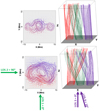 |
Fig. 1. Illustration of the magnetic field line complexity for IC1 (upper row) and IC2 (lower row) showing the projection of the magnetic field lines onto the xy-plane (left column) and the configuration of representative field lines in 3D (right column), modified from Howson et al. (2020). The LOS angles (LOS1, 2, 3 and 4), used in the forward modelling, are green arrows if they are in the xy-plane (left) and purple in the xz-plane (right). |
The numerical simulations in Howson et al. (2020) and Reid et al. (2018) use the Lagrangian-remap code, Lare3D (Arber et al. 2001), which solves the fully 3D normalised non-ideal MHD Equations. In Howson et al. (2020), the effects of thermal conduction, optically thin radiation and gravity were neglected. The background viscosity was set to zero, however, to ensure numerical stability, the Lare3D code does include shock viscosity. This contributes to both the viscous force and viscous heating term. The simulations were non-resistive (η = 0) and hence, the only increases in temperature are due to compression and the (small) shock viscosity heating term.
We refer to the numerical simulations of Howson et al. (2020) as S1 and S2 (corresponding to initial conditions IC1 and IC2, respectively). The numerical domain has dimensions of 30 Mm × 30 Mm × 100 Mm, using a numerical grid of 256 × 256 × 1024 cells.
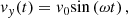
The transverse waves investigated in Howson et al. (2020) are excited by imposing a wave driver on the lower z boundary of the form v(t) = (0,vy,0), where vy is defined by
with an amplitude, v0 ≈ 20 km s−1 and frequency, ω ≈ 0.21 s−1. This corresponds to a wave period of τ ≈ 28 s. A relatively high frequency driver is implemented to allow multiple wavelengths to fit within the length of the numerical domain (100 Mm). Although the majority of wave or oscillatory periods observed in the solar corona are of the order of a few minutes (e.g. Tomczyk et al. 2007; Tomczyk & McIntosh 2009; Morton et al. 2016), observations of wave periods of a few tens of seconds have also been identified along coronal loops (e.g. Williams et al. 2001) and spicules (e.g. Okamoto & De Pontieu 2011; Yoshida et al. 2019).
The x and y boundaries are periodic and the z boundaries set the gradients of all the variables to be zero, with the exception of the velocity, where the wave driver is imposed on the bottom boundary and the velocity is set to zero on the top. This ensures that waves are reflected at the top boundary and forced to propagate back into the domain.
2.2. Evolution
In order to interpret the synthetic emission data generated by the forward modelling (see Sect. 3), it is helpful to first briefly discuss the evolution of the system, in particular the behaviour of the velocity, temperature and density.
One significant feature seen in Howson et al. (2020) was the presence of phase mixing, where the formation of small length scales depends on the amount of magnetic field complexity. The left-hand panels of Figs. 2a and b are snapshots of vy before the first reflection off the top boundary. They each show the distortion of the (velocity) wave front as it propagates through the complex magnetic field. The degree of distortion clearly relates to the amount of braiding (complexity) of the magnetic field, that is to say the more complex the field the greater the level of phase mixing. The last two panels in Figs. 2a and b illustrate the behaviour of the waves at a later time (t = 239 s), when they have reflected back into the domain and begin to generate wave interference.
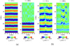 |
Fig. 2. Contour plot of vy in a vertical slices through y = 0 Mm at 141 s (first panels) and 239 s (second panels) for simulations (a) S1 and (b) S2. The range of the colour bars change between some panels. |
Although the imposed boundary driver is incompressible, non-linearity and coupling to fast modes lead to compressibility as the waves propagate through the domain. Figure 3 illustrates the complex and compressible nature of the velocity field through a horizontal slice at the midplane in S2. Clearly, the velocity is no longer aligned with the boundary wave driver. This (partial) change to the polarisation of the wave, from vy to vx, is due to the interaction of the perturbations in By with jz, which produces an x-component of the Lorentz force (see also Howson et al. 2019b) and hence, generates velocity perturbations in the x-direction, as the waves travel along the twisted magnetic field lines.
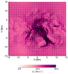 |
Fig. 3. Illustration of the speed (contours) and the horizontal velocity (vectors) through the horizontal midplane for S2 at t = 239 s. |
The density and temperature profiles averaged along the three main axes are illustrated in Figs. 4 and 5 for simulations S1 and S2, respectively (where the scale of the colour bar changes between S1 and S2). Initially, a tube-like structure is present in both simulations when viewing along the x and y-axes. These are regions of higher temperature, compared to the surroundings, and occur where the viscous and Ohmic heating is largest in Reid et al. (2018). Due to pressure balance and the larger temperatures, there is a drop in density within the tube-like structures (see Howson et al. 2019a). Therefore, in this case, the Alfvén speed is generally higher inside the magnetic structures than outside. This is converse to what is typically used in wave studies and is more common for structures in the lower atmosphere but has also been studied in a coronal context (e.g. Howson et al. 2019b). Although in S1 the right-hand thread is a distinct structure (see Fig. 1), this is only apparent in the temperature and density averaged along the z-axis and is not evident when averaging along the x and y-axes.
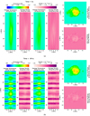 |
Fig. 4. Contours of average temperature (rainbow) and density (pink) along the three axes at (a) 0 s and (b) 974 s for S1. |
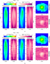 |
Fig. 5. Contours of average temperature (rainbow) and density (pink) along the three axes at (a) 0 s and (b) 974 s for S2. |
As the simulations evolve, the compressible nature of the velocity field becomes evident in Figs. 4b and 5b, where we see perturbations in both the density and temperature along the x and y-axes. As discussed above, in the initial equilibria, regions of high temperature typically coincide with low density plasma. However, for the perturbations seen in Figs. 4b and 5b, we see a co-spatial increase (or decrease) in both the temperature and the density. As such, they highlight regions of adiabatic heating (or cooling). In S1, these perturbations form horizontally across the plane-of-the-sky (POS) and obscure the initial structures. In S2, on the other hand, they predominantly appear in regions where |x| and |y| > 8 Mm and do not obscure the initial density and temperature configuration. This is due to the deformed nature of the wave front at later times in S2, implying that regions of compression (or rarefaction) associated with the wave do not necessarily align along the line-of-sight (LOS), resulting in weaker LOS density (and temperature) perturbations.
3. Forward modelling
3.1. Emission lines and LOS
To produce the synthetic emission data, the numerical results are forward modelled using the FoMo code (Van Doorsselaere et al. 2016). This generates optically thin EUV and UV emission lines using the CHIANTI atomic database (Dere et al. 1997; Landi et al. 2013).
We choose to model the Fe XII 193Å and Fe XVI 335Å emission lines, as these provide good coverage of the temperature range in our simulations. The rest wavelengths are 193.509 Å and 335.409 Å, with peak formation temperatures of log(T) = 6.20(∼ 1.57 MK) and log(T) = 6.42(∼ 2.65 MK), respectively.
We examine four different LOS angles which are illustrated in Fig. 1 and Table 1. Two of the angles lie in the xy-plane and cut across the magnetic flux tubes (LOS1 and 2) whereas LOS3 and LOS4 lie in the xz-plane and are approximately aligned with the magnetic structure. The LOS3 viewing angle is directly aligned with the axis of the loop, which could occur near disc centre in the lower atmosphere.
LOS angles given in reference to their plane of the sky (POS) and the axis they are parallel to.
The numerical grid used in Howson et al. (2020) was modified in this forward modelling analysis to reduce computational costs by spatially resampling the original simulations to every fourth grid cell along x, y and z. The temporal resolution was not altered. From examining a selection of the data at full spatial resolution, we confirmed that the spatial re-sampling had no significant impact on the forward modelling results.
3.2. Imaging signatures
Figures 6 and 7 illustrate the synthetic total intensity at two instances in time (t = 0 s and t = 974 s) in Fe XII and Fe XVI. We show results for both simulations, along LOS1 (Fig. 6) and LOS2 (Fig. 7). Fe XVI generally detects the hotter plasma, that is to say initially the central column and later on, in the regions where we observed adiabatic heating. Of course, if the plasma density is low, then even in regions of hot plasma, the Fe XVI intensity will also be low. An example of this can be seen in the S2 simulation (last column of Fig. 6; |x| ≲ 7 Mm, − 35 Mm ≲ y ≲ 40 Mm). The low intensity in the cooler line, for S2, is a combination of low density and plasma being outwith the formation temperature of Fe XII (third column of Figs. 6 and 7). Apart from this, the Fe XII intensity is essentially the “inverse” of Fe XVI.
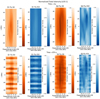 |
Fig. 6. Normalised total intensity for S1 and S2 in Fe XII and Fe XVI looking along LOS1 at 0 s (row 1) and 974 s (row 2). In each case, the intensities have been normalised by their own spatio-temporal maximum. |
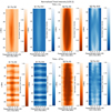 |
Fig. 7. Normalised total intensity for S1 and S2 in Fe XII and Fe XVI looking along LOS2 at 0 s (row 1) and 974 s (row 2). In each case, the intensities have been normalised by their own spatio-temporal maximum. |
We note that the complexity in the equilibrium configuration is not evident from the intensity contours at t = 0 (see, for example, Pontin et al. 2017). The hotter line for simulation S1 is the only case where a flux tube-like structure is even detected. As expected, there are no signs of the two threads in S1 which became unstable during the Reid et al. (2018) simulation. However, there are also no signs of the third thread, which is still distinguishable along LOS1 when examining the traced magnetic field lines in Fig. 1.
Due to the compressible nature of the waves, we do expect to see some intensity changes, associated with the density and temperature perturbations discussed above. Indeed, as the simulations progress, the presence of waves becomes most apparent for the least complex magnetic field configuration (see the first and second panel on the bottom row of Figs. 6 and 7), where we saw the clearest density and temperature perturbations. For the more complex field (third and fourth panels), the wave-like behaviour is less apparent and could be mistaken for background noise. Figure 8, which shows the running difference of the total intensity (i.e. the difference between subsequent time steps with a cadence of 3.6 s), has the same properties. We see a clear signature of the waves in both lines for S1 (first two panels). This change in intensity highlights the compressible nature of the velocity field despite the incompressible nature of the boundary driver. However, for the more braided field (S2 – last two panels), the running difference does not reveal the wave dynamics either, due to the complex and continuously changing nature of the wave front.
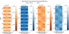 |
Fig. 8. Normalised running difference of total intensity (with a cadence of 3.6 s) for S1 and S2 in Fe XII and Fe XVI looking along LOS1 at 974 s. In each case, the running-differences have been normalised by their own spatio-temporal maximum. |
In addition to the running difference, we investigate the base difference, that is to say we subtract the initial intensity from the intensity at each time step. This is shown in the first panel of Fig. 9a. We observe minor changes in the intensity profile near the start of the simulations as illustrated at 43 s during S2 (first panel). These changes coincide with the front of the Alfvénic wave (at z ≈ −20 Mm) seen in the Doppler velocity in the second panel (a more in-depth analysis of the Doppler velocity is given in Sect. 3.3). The presence of a slow wave, generated by the boundary driver, can also be seen in the left-hand panel, propagating behind the transverse wave with a wave front at z ≈ −40 Mm. These perturbations to the intensity are caused by the compression and rarefaction of the plasma as a result of the waves. Intriguingly, the horizontal spatial scales of the slow wave (seen in the base difference), are smaller than those seen in the transverse wave (shown by the Doppler velocity). This is due to the way the boundary driver (vy) interacts with the y-component of the magnetic field on the bottom boundary. The schematics in Fig. 10 helps to explain why this is the case. When Byvy > 0, the slow wave component (“Slow” in Fig. 10) acts along the magnetic field, causing compression, whereas when Byvy < 0, the slow component is now anti-parallel to the magnetic field, resulting in rarefaction of the plasma. In Fig. 9b, we show the configuration of By on the bottom boundary of the domain. We see that the sign of By broadly aligns with the small spatial scale features seen in the base difference and matches the compression and rarefaction pattern illustrated in Fig. 10.
 |
Fig. 9. First and second panel of (a) illustrate the total relative intensity base difference and Doppler velocity, respectively, in Fe XVI along LOS1 in S2. Depicted in (b) is By on the bottom z boundary. The black line represents the By = 0 G contour. In (a) and (b) the white dashed lines highlight the location of the small horizontal spatial features. All panels are at 43 s. |
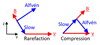 |
Fig. 10. Illustration of the compression and rarefaction due to the slow wave, seen in the intensity base difference in Fig. 9a. All vectors are projected onto the yz-plane, where B is the magnetic field on the lower boundary, v = (0, vy, 0) is the boundary driver and Alfvén and Slow are the Alfvén and slow components of the propagating wave. |
The figures of intensity and running difference along LOS1 and 2 (Figs. 6–8), do not show obvious signs of magnetic field complexity. This also holds for the intensity along LOS3 (Fig. 11a). However, when examining the running difference along LOS3 (Fig. 11b), the small scale spatial structuring becomes apparent. This helps identify regions of complex field but does not imply that other regions are not complex. For example, Fe XII S2 (Fig. 11b – bottom left panel) does not show small scale structures in the centre, despite complex field being present (compare to bottom left panel of Fig. 1). Hence, if observing the Fe XII emission in isolation, one could incorrectly conclude that the S1 magnetic field is more intricate. Similarly, when examining the Fe XVI synthetic emission in isolation (Fig. 11b – right column), even though it shows the regions of complex magnetic field projected onto the plane of the sky (compare to left column of Fig. 1), distinguishing the intricacy of the two magnetic fields (S1 and S2) is not straightforward. Therefore, a comparison of the complexity of the two magnetic field configurations from the intensity images does not necessarily give the correct results.
 |
Fig. 11. Normalised (a) total intensity and (b) running difference (with a cadence of 3.6 s) along LOS3 in Fe XII (first column) and Fe XVI (second column) in both S1 (first row) and S2 (second row) at 974 s. Quantities in each panel have been normalised by their own spatio-temporal maximum. |
One intriguing feature visible in the running difference of intensity along LOS3 and 4 during the first transit of the transverse waves through the domain, is the presence of an apparent rotational motion (see movie1). This is not indicative of real torsional motions, which are not present within the plasma but instead is caused by compressible wave fronts propagating along twisted field. In Fig. 12, we have illustrated this behaviour by tracking one contour level of the running difference at consecutive times during S2 (it is also seen in S1). Along LOS3, we see an apparent anticlockwise rotation but by altering the viewing angle by just 10° (LOS4), the rotational motion is hardly observable. For tilted viewing angles, the upward propagation of waves from the lower boundary (a motion from right to left in the left panel of movie1 and the bottom row of Fig. 12) obscures the apparent rotation.
 |
Fig. 12. Single contour level of the normalised running difference of the total intensity (with a cadence of 3.6 s) along LOS3 (row 1) and LOS4 (row 2) in Fe XVI during S2 at 14 (red), 21 (blue), 28 (green) and 36 (purple) seconds. Associated movie is available online. |
In addition, this apparent torsional motion is only visible during the initial transit of the waves through the domain, that is to say before the first reflection off the top boundary. Once the waves reflect, the interference between the counter-propagating waves leads to random and chaotic patterns. Hence, this apparent rotational motion is probably unlikely to be observed, for example in closed coronal loops, due to the constant motions and waves propagating along magnetic field lines which is causing wave interference. However, in cases where there is a significant difference in the outward and inward propagating wave power (e.g. Verth et al. 2010; Tiwari et al. 2019) or in open magnetic field regions (e.g. Morton et al. 2015), this apparent rotational motion may lead to misinterpretations of torsional wave modes.
3.3. Spectral signatures
Even though there is a weak compressible aspect to the waves, they do not show strong signatures in intensity. In addition, increased LOS cancellation for the more braided simulation leads to very weak, if any, detectable signs of wave propagation in the S2 simulation (last two panels in lower rows of Figs. 6 and 7 and final two panels in Fig. 8).
However, we are able to clearly detect the presence of waves using Doppler velocities. In Fig. 13, we illustrate the Doppler velocities observed with the Fe XVI line along LOS1. These are obtained by fitting a (single) Gaussian to the specific intensity and measuring the shift of the Gaussian peak from the rest wavelength. The times in the first two panels coincide with Fig. 2b and the remaining two panels show later times in the simulation, when the wave interference and phase mixing are well-developed. At all times, propagating waves are clearly present as perturbations in the Doppler velocities. The magnitudes of the Doppler shifts are somewhat large in comparison to actual observations. However, when an integration time of 10 s (similar to that of modern spectrometers) was used, we found a decrease in the values of the Doppler shift by a factor of almost two. The structure of the Doppler velocity profiles were largely unaltered.
 |
Fig. 13. Doppler velocity for S2 along LOS1 in Fe XVI. The range of the colour bars change between each panel. |
We note that in S2, a single Gaussian could not be fitted to a very small percentage (less than ∼0.06%) of the line profiles. These instances all occur at later times in the simulation when multiple, more complex plasma flows are present along the LOS, resulting in complex, double (or more) peaked line profiles. As this only happens in a very small number of cases, it does not affect the analysis of the data presented here.
Before the transverse waves reflect off the top boundary (t = 141 s), we see (weak) phase mixing as described in Howson et al. (2020) and in Sect. 2.2. The level of complexity is evident by contrasting S2 with S1 using the same emission line (compare the left hand panel of Fig. 13 and 14). As expected, the level of distortion to the wave front is greater in S2, confirming that the more complex field leads to more phase mixing. When comparing the S2 Doppler velocities in Fe XII (Fig. 15) and in Fe XVI (first panel Fig. 13), there is more phase mixing evident in the hotter line. This is due to the temperature profile of the background magnetic field. In general, the more complex field (which enhances phase mixing) has higher local temperatures. The cooler lines, on the other hand, mostly detect regions where the field is less complex, and thus, exhibit less wave distortion.
 |
Fig. 14. Doppler velocity from S1 in Fe XVI at 141 s along LOS1. |
 |
Fig. 15. Doppler velocity from S2 in Fe XII at 141 s along LOS1. |
Looking more closely at a small region of panel two in Fig. 13, as illustrated in Fig. 16, an out of phase red-blue structure is detected. Assuming no prior knowledge of this simulation (i.e. the magnetic field configuration and the polarisation of the boundary driver) and a field of view limited to this small region, one could misinterpret this Doppler velocity configuration as torsional motions.
 |
Fig. 16. Doppler velocity for S2 along LOS1 in Fe XVI (left panel), repeated from panel 2 of Fig. 13. A zoomed in region of the domain (right panel) where −7 Mm ≤ z ≤ 50 Mm and the other axis is between −3 Mm and 12 Mm. The range of the colour bars change between each panel. |
Similar Doppler velocity features have been identified by various authors in observational data. For example, Srivastava et al. (2017) find a similar signature when examining the Doppler velocity of a highly structured magnetic flux tube, using SST/CRISP in the Hα 6562.8Å spectral line which was interpreted as torsional oscillations. Kohutova et al. (2020) also interpret such alternating red-blue shifts along the edges of a flux tube as torsional Alfvén oscillations. However, in our simulations, these specific Doppler velocity patterns are the result of phase mixing and counter-propagation of transverse waves in a complex magnetic field rather than actual torsional waves.
Figure 17 illustrates the LOS2 Doppler velocities at the same times as the LOS1 Doppler velocities in Fig. 13. The change in the wave polarisation, discussed in Howson et al. (2019b) and Sect. 2.2, is evident when comparing the Doppler shifts along the different LOS angles. Energy is transferred from the vy component (observable in LOS1) of the velocity field near the bottom boundary to a vx component (observable in LOS2) as time progresses. From the first panel, we see that as the waves propagate up through the domain, the change in polarisation becomes more pronounced, resulting in the Doppler velocities in LOS2 increasing with height.
 |
Fig. 17. Doppler velocity for S2 along LOS2 in Fe XVI. The range of the colour bars change between each panel. |
In LOS2, the spatial profile of the Doppler velocities in many locations is not dissimilar to the out of phase red-blue shifts seen in Fig. 16. Again, caution is needed to avoid misinterpreting these signatures of phase mixing as torsional motions. The LOS2 Doppler velocity signatures are quite complex and intricate, given that our boundary velocity driver is in fact a simple sinusoidal driver. Hence, complex observational signatures do not necessarily imply the presence of a complex driver but may instead (as in the case here) be indicative of a complex background magnetic field structure. When examining LOS2 in S1 (Fig. 18), we find largely the same behaviour as in S2, except over a narrower region as less of the domain contains complex magnetic field structures (see top left hand panel of Fig. 1).
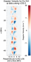 |
Fig. 18. Doppler velocities for Fe XVI in S1 at 890 s along LOS2. |
Figure 19 shows the evolution of the mean magnitude of the Doppler velocity along LOS2 during both simulations, in both emission lines. It is clear that at all times and irrespective of the emission line, the values of the Doppler velocities are smaller for the S1 simulation. This is due to the less complex magnetic field structure in S1, which leads to a smaller transfer of energy to the x component of the velocity field (Fig. 20), and hence smaller Doppler velocities along LOS2. Figure 20 shows the mean magnitudes of the vy and vx velocity components for both simulations. At early stages, the behaviour of vy is almost identical. Following the first reflection off the top boundary (∼150 s), the oscillation amplitudes increase and we see vy (solid blue and green lines) deviate in both simulations, as more energy is transferred to vx in S2 (dashed blue line) due to the more complex magnetic field.
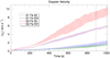 |
Fig. 19. Mean magnitude of the Doppler velocity along LOS2 from S1 (green and blue) and S2 (red and purple) in Fe XII (green and red) and Fe XVI (blue and purple) as a function of time. The vertical black dashed line marks t = 890 s corresponding to the second panel of Figs. 17 and 18. |
3.4. Kinetic energy budget
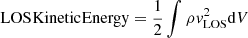
In this section, we compare the kinetic energy in both simulations to the estimated kinetic energy obtained from the synthetic emission data, that is to say using the Doppler velocities calculated in Sect. 3.3. Figure 21 illustrates the evolution of these kinetic energies in both simulations (S1 and S2), along LOS1 and 2. The volume integrated LOS kinetic energy (turquoise line) is calculated from the simulation results by setting vLOS = vy or vx, in Eq. (1), for LOS1 and 2, respectively:
 (1)
(1)
 (2)
(2)
To estimate the kinetic energies from the spectroscopic information (red and blue lines), we use Eq. (2), where L is the LOS depth,  is the average density, and vD is the Doppler velocity for a given emission line, all along the LOS. We note that all the kinetic energies in Fig. 21 have been smoothed to better illustrate their general evolution rather than the amplitude of the oscillations.
We realise that the depth, L, and density profile along the LOS are not easily measured from coronal observations. The length is simply a scaling factor which does not change the behaviour of the estimated kinetic energies. However, a reasonable estimate is required for comparison with the actual volume integrated kinetic energy. For the density, we require the average value along the LOS. This can be estimated using line ratios as a density diagnostic tool (e.g. Dere et al. 1979; Mason et al. 1979; Landi & Miralles 2014; Polito et al. 2016).
Using a value of L equal to 30 Mm (i.e. the depth of our numerical domain), we can see that when we observe along the direction of the boundary driver (LOS1), the “observed” kinetic energy is a less accurate representation of the true (total) kinetic energy as the complexity of the field increases (i.e. S2 is less accurate than S1 along LOS1 – see left column of Fig. 21). This is a result of the increased polarisation change in the S2 simulation where more energy is transferred from vy to vx (see Fig. 20) and hence we find a less accurate estimate of the total kinetic energy. Even so the estimates are, at worst, about 50% of the total value.
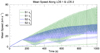 |
Fig. 20. Mean magnitude of vy (LOS1 solid lines) and vx (LOS2 dashed lines) in S1 (green) and S2 (blue) as a function of time. The vertical black dashed line marks t = 890 s corresponding to the second panel of Figs. 17 and 18. |
Not only does the complexity of the magnetic field alter the estimated kinetic energy but the LOS angle has a significant effect as well. Comparing the left-hand and right-hand columns of Fig. 21, we see that for the LOS perpendicular to the boundary driver (i.e. LOS2) the estimated kinetic energies are up to several orders of magnitude less than the total kinetic energy (compare blue line in top right panel with green line in top left panel of Fig. 21). As time progresses, and the polarisation of the wave changes, we observe an increase in the estimates along LOS2 and the estimated kinetic energies along LOS1 begin to deviate from the true total kinetic energy.
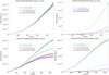 |
Fig. 21. Total (green) and LOS (turquoise) kinetic energy is integrated over the full 3D numerical domain compared to the estimated kinetic energy in Fe XII (blue) and Fe XVI (red), during S1 (row 1) and S2 (row 2) along LOS1 (column 1) and LOS2 (column 2). All curves have been smoothed to illustrate the general trend rather than the amplitude of the oscillations. The total kinetic energy has not been plotted in panel b as it is several orders of magnitude larger (but the total kinetic energy is the same as in panel a). |
As well as underestimating the total kinetic energy in the 3D domain, the estimated kinetic energy also underestimates the LOS kinetic energy. This is due to a combination of only sampling regions which are within the formation temperature range for the selected emission line and cancellation of velocities along the LOS. The energy which is “lost” due to multiple plasma flows along the LOS, caused by the complex magnetic field, would result in an increased non-thermal line width of the specific intensity (see also e.g. McIntosh & De Pontieu 2012). Similarly, Pant et al. (2019) investigate the discrepancy between the observed wave energy, calculated from the Doppler velocities, and the true wave energy and find that the additional energy is present in the non-thermal line widths. Figure 22 shows the evolution of the average line width, calculated using the full-width-half-maximum (FWHM) of the specific intensity, for simulation S2. Since the average temperature during the simulation does not change significantly over time, the thermal line width remains approximately constant throughout the simulation. Hence, the increase in the line width confirms that some of the “lost” energy is indeed hidden in the non-thermal line width.
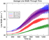 |
Fig. 22. Average line width, using the FWHM, as a function of time during S2. We show LOS1 (green and blue) and LOS2 (red and purple) in Fe XII (green and red) and Fe XVI (blue and purple). |
4. Discussion and conclusions
In this paper, we have examined the synthetic emission data for two 3D MHD simulations which model the propagation and interference of transverse waves in complex magnetic fields, where the two simulations differ in the complexity of the initial background field. Waves are excited by a sinusoidal, transverse driver imposed at the bottom boundary and over time, are distorted by complex interference and phase mixing.
For LOS1 and LOS2 (Fig. 1 and Table 1), the total intensity largely corresponded to the temperatures in the domain. The Fe XVI line captures the hotter central column of plasma, where the strongest braiding of the magnetic field is present, as well as locations of adiabatic heating. The cooler Fe XII line essentially detected the “inverse” of Fe XVI, that is to say the cooler outer regions of the simulation domain and, as the simulation progressed, locations of rarefaction. The magnetic field complexity was not associated with similar intricate structuring in the intensities along LOS1 and LOS2. The only evidence of complexity in the magnetic field was identified by examining the running differences along the magnetic field structure (LOS3 and 4). Regions of complex field could be detected using careful analysis of multiple emission lines but even then, an absolute comparison of the level of fine-scale structuring in the two simulations was not possible. In the S1 simulation (less braiding), tracing the magnetic field lines showed that one of the flux tubes is still distinguishable in the initial setup. However, with the exception of the Fe XVI line along LOS3, the integrated intensities showed little evidence of the presence of this structure.
Despite the incompressible nature of the boundary driver, due to non-linearity and coupling to compressive wave modes, the waves are detectable in the LOS intensities. For S1, there are indeed (weak) signatures in the intensity and running difference (of the intensities) in both Fe lines. However, for the more complex field in S2, the wave front is substantially deformed and compressibility occurs on smaller spatial scales, leading to increased cancellation of the density and temperature perturbations along the LOS. As a result, the wave propagation is barely detectable and could easily be mistaken for background noise. In addition to the transverse waves, (compressible) slow waves also enter the domain. Here, we found additional structuring in the wave fronts in the horizontal direction compared to the transverse waves. These shorter horizontal spatial scales of the slow wave were most easily visible in the intensity base differences and are caused by the interplay between the direction of the driver and the direction of the local magnetic field. Of course, a different driver and/or local magnetic field topology would lead to different horizontal structuring.
During the first transit of the wave through the domain, we see an apparent rotational motion in the intensity running difference along LOS3, even though none are actually present in the domain. However, changing the LOS angle by just 10°, results in this apparent motion being much harder to detect, although the effect of a minor change to the viewing angle on the observations may be overcome by removing the average background propagation of the running difference structure. This apparent rotation also vanishes once the waves reflect off the top boundary and the wave interference results in a random chaotic pattern in the intensity running differences. It is therefore unlikely that this apparent rotational motion would be an issue in the interpretation of waves in closed magnetic structures, particularly given the presence of wave interference. However, in open field regions or where wave propagation is largely unidirectional (e.g. due to strong damping along the structure or efficient transmission at one of the footpoints), distinguishing transverse and rotational motions might not always be trivial and it is useful to be aware of the potential for misinterpretation when analysing wave propagation through complex magnetic field structures.
The strongest signature of the transverse waves was present in the Doppler velocities. For the more complex field, we see more phase mixing, evident from the distortion of the wave fronts (Howson et al. 2020). This was especially visible in the hotter Fe XVI line, since the hotter plasma corresponds to regions of more complex magnetic field. After the waves reflect off the top boundary, the combination of phase mixing and wave interference of upward and downward propagating waves throughout the domain leads to extensive distortion of the wave fronts. The Doppler shift patterns become increasingly fine-structured and chaotic, complicating the interpretation of the nature of the wave mode. Indeed, at certain instances along LOS1, the Doppler shifts could again be misinterpreted as torsional motions. Similar side-by-side red-blue signatures were also present along LOS2 once the polarisation of the wave changed to a mixture of vy (the direction of the boundary driven waves) and vx. Comparable Doppler velocity profiles are identified in Goossens et al. (2014) although for a different numerical set up. In particular, the authors investigate the synthetic emission from an over dense plasma cylinder in a uniform magnetic field, with an imposed velocity field replicating the behaviour of the kink wave. Observations along the direction of the transverse motion show red shift in the location of the internal plasma and blue shift in the external plasma. This red-blue structure is similar to our observations along LOS1. They also examine the LOS perpendicular to the transverse motion of the kink wave. Again, red-blue Doppler shift structures are formed. However, this time they appear to be the signatures of a directly driven torsional Alfvén wave, rather than simply the azimuthal component of a kink mode.
Using the synthetic spectroscopic data, we estimated the kinetic energy in the simulations. We considered the effects of various factors, including the LOS angle, magnetic field complexity and the emission lines (Fe XII and Fe XVI). In the most optimal configuration, where the LOS is parallel to the boundary driver (LOS1) and the magnetic field is less braided (S1), we achieved reasonably accurate estimates for the total kinetic energy. However, for the least optimal configuration, namely a LOS perpendicular to the driver (LOS2 in the S1 case), we attain estimates several orders of magnitude less than the physical value. In practice, estimates of the total kinetic energy are likely to be between these two cases and could underestimate the true kinetic energy by an order of magnitude, where some of this energy will be represented by enhanced non-thermal line widths (e.g. McIntosh & De Pontieu 2012; Pant et al. 2019). Of course, additional uncertainties in the density profile and the LOS integration length may further increase the uncertainty in the energy measurements. In a previous study, De Moortel & Pascoe (2012) use a simple 3D numerical model of wave propagation along multiple loop strands to examine the effect of LOS integration on estimating the energy budget. They use a more complex driver than the one presented in this article, which is designed to mimic random footpoint motions. This may also have an effect on the energy budget, given that we found substantially different estimates from a LOS parallel to a LOS perpendicular to our unidirectional driver (i.e. a simple back and forth driver along one direction, in this case the y-axis). In their study, the authors find that the LOS kinetic energy budget captures, at best, 40% of the actual kinetic energy generated, suggesting that the LOS integration has a substantial impact on the kinetic energy estimated from Doppler shifts.
In summary, many of the observables we have discussed in this paper are relatively easily understood, at least with the knowledge of the evolution of the physical parameters in the 3D domain. However, our analysis does highlight that care is required in some instances, where the propagation of a simple wave front in a complex magnetic field can lead to complex patterns in the observables. In particular, we found that when considering the intensities or Doppler velocities in isolation, distinguishing between transverse and rotational motions is not always trivial. Finally, we investigated the estimated kinetic energy which is highly dependent on the spatial scale of the wave driver, the polarisation of the wave, complexity of the background field and the LOS angles.
Movie
Movie of Fig. 12 Access Supplementary Material
Acknowledgments
The authors would like to thank Paola Testa, Jorrit Leenaerts and Vaibhav Pant for helpful discussion on the double-Gaussian fitting routines. We would also like to thank Patrick Antolin and Tom Van Doorsselaere for assistance with the FoMo code. The research leading to these results has received funding from the UK Science and Technology Facilities Council (consolidated Grants ST/N000609/1 and ST/S000402/1) and the European Union Horizon 2020 research and innovation programme (Grant agreement No. 647214). IDM acknowledges support from the Research Council of Norway through its Centres of Excellence scheme, project number 262622.
References
- Anfinogentov, S. A., Nakariakov, V. M., & Nisticò, G. 2015, A&A, 583, A136 [NASA ADS] [CrossRef] [EDP Sciences] [Google Scholar]
- Antolin, P., & Van Doorsselaere, T. 2013, A&A, 555, A74 [NASA ADS] [CrossRef] [EDP Sciences] [Google Scholar]
- Arber, T. D., Longbottom, A. W., Gerrard, C. L., & Milne, A. M. 2001, J. Chem. Phys., 171, 151 [Google Scholar]
- Arregui, I. 2015, Phil. Trans. R. Soc. London, Ser. A, 373, 20140261 [Google Scholar]
- Aschwanden, M. J., Fletcher, L., Schrijver, C. J., & Alexander, D. 1999, ApJ, 520, 880 [NASA ADS] [CrossRef] [Google Scholar]
- Aschwanden, M. J., De Pontieu, B., Schrijver, C. J., & Title, A. M. 2002, Sol. Phys., 206, 99 [NASA ADS] [CrossRef] [Google Scholar]
- Browning, P. K., Gerrard, C., Hood, A. W., Kevis, R., & van der Linden, R. A. M. 2008, A&A, 485, 837 [NASA ADS] [CrossRef] [EDP Sciences] [Google Scholar]
- Cargill, P. J., De Moortel, I., & Kiddie, G. 2016, ApJ, 823, 31 [NASA ADS] [CrossRef] [Google Scholar]
- Chen, F., & Peter, H. 2015, A&A, 581, A137 [NASA ADS] [CrossRef] [EDP Sciences] [Google Scholar]
- Cranmer, S. R., & van Ballegooijen, A. A. 2005, ApJS, 156, 265 [NASA ADS] [CrossRef] [Google Scholar]
- De Moortel, I., & Browning, P. 2015, Phil. Trans. R. Soc. London, Ser. A, 373, 20140269 [Google Scholar]
- De Moortel, I., & Nakariakov, V. M. 2012, Phil. Trans. R. Soc. London, Ser. A, 370, 3193 [Google Scholar]
- De Moortel, I., & Pascoe, D. J. 2012, ApJ, 746, 31 [NASA ADS] [CrossRef] [Google Scholar]
- Dere, K. P., Mason, H. E., Widing, K. G., & Bhatia, A. K. 1979, ApJS, 40, 341 [NASA ADS] [CrossRef] [Google Scholar]
- Dere, K. P., Landi, E., Mason, H. E., Monsignori Fossi, B. C., & Young, P. R. 1997, A&AS, 125, 149 [NASA ADS] [CrossRef] [EDP Sciences] [Google Scholar]
- Duckenfield, T., Anfinogentov, S. A., Pascoe, D. J., & Nakariakov, V. M. 2018, ApJ, 854, L5 [NASA ADS] [CrossRef] [Google Scholar]
- Goossens, M., Soler, R., Terradas, J., Van Doorsselaere, T., & Verth, G. 2014, ApJ, 788, 9 [NASA ADS] [CrossRef] [Google Scholar]
- Heyvaerts, J., & Priest, E. R. 1983, A&A, 117, 220 [NASA ADS] [Google Scholar]
- Hillier, A., Morton, R. J., & Erdélyi, R. 2013, ApJ, 779, L16 [NASA ADS] [CrossRef] [Google Scholar]
- Hood, A. W., Browning, P. K., & van der Linden, R. A. M. 2009, A&A, 506, 913 [NASA ADS] [CrossRef] [EDP Sciences] [Google Scholar]
- Howson, T. A., De Moortel, I., Reid, J., & Hood, A. W. 2019a, A&A, 629, A60 [NASA ADS] [CrossRef] [EDP Sciences] [Google Scholar]
- Howson, T. A., De Moortel, I., Antolin, P., Van Doorsselaere, T., & Wright, A. N. 2019b, A&A, 631, A105 [CrossRef] [EDP Sciences] [Google Scholar]
- Howson, T. A., De Moortel, I., & Reid, J. 2020, A&A, 636, A40 [CrossRef] [EDP Sciences] [Google Scholar]
- Karamimehr, M. R., Vasheghani Farahani, S., & Ebadi, H. 2019, ApJ, 886, 112 [CrossRef] [Google Scholar]
- Klimchuk, J. A. 2006, Sol. Phys., 234, 41 [NASA ADS] [CrossRef] [Google Scholar]
- Klimchuk, J. A. 2015, Phil. Trans. R. Soc. London, Ser. A, 373, 20140256 [Google Scholar]
- Kohutova, P., Verwichte, E., & Froment, C. 2020, A&A, 633, L6 [NASA ADS] [CrossRef] [EDP Sciences] [Google Scholar]
- Landi, E., & Miralles, M. P. 2014, ApJ, 780, L7 [NASA ADS] [CrossRef] [Google Scholar]
- Landi, E., Young, P. R., Dere, K. P., Del Zanna, G., & Mason, H. E. 2013, ApJ, 763, 86 [NASA ADS] [CrossRef] [Google Scholar]
- Longbottom, A. W., Rickard, G. J., Craig, I. J. D., & Sneyd, A. D. 1998, ApJ, 500, 471 [NASA ADS] [CrossRef] [Google Scholar]
- Longcope, D. W., & Sudan, R. N. 1994, ApJ, 437, 491 [NASA ADS] [CrossRef] [Google Scholar]
- Magyar, N., & Nakariakov, V. M. 2020, ApJ, 894, L23 [CrossRef] [Google Scholar]
- Mason, H. E., Bhatia, A. K., Doschek, G. A., & Feldman, U. 1979, A&A, 73, 74 [Google Scholar]
- McIntosh, S. W., & De Pontieu, B. 2012, ApJ, 761, 138 [NASA ADS] [CrossRef] [Google Scholar]
- McIntosh, S. W., de Pontieu, B., Carlsson, M., et al. 2011, Nature, 475, 477 [NASA ADS] [CrossRef] [Google Scholar]
- Morton, R. J., Tomczyk, S., & Pinto, R. 2015, Nat. Comm., 6, 7813 [Google Scholar]
- Morton, R. J., Tomczyk, S., & Pinto, R. F. 2016, ApJ, 828, 89 [NASA ADS] [CrossRef] [Google Scholar]
- O’Hara, J. P., & De Moortel, I. 2016, A&A, 594, A67 [NASA ADS] [CrossRef] [EDP Sciences] [Google Scholar]
- Okamoto, T. J., & De Pontieu, B. 2011, ApJ, 736, L24 [NASA ADS] [CrossRef] [Google Scholar]
- Okamoto, T. J., Tsuneta, S., Berger, T. E., et al. 2007, Science, 318, 1577 [NASA ADS] [CrossRef] [PubMed] [Google Scholar]
- Pagano, P., & De Moortel, I. 2017, A&A, 601, A107 [NASA ADS] [CrossRef] [EDP Sciences] [Google Scholar]
- Pagano, P., & De Moortel, I. 2019, A&A, 623, A37 [NASA ADS] [CrossRef] [EDP Sciences] [Google Scholar]
- Pagano, P., Pascoe, D. J., & De Moortel, I. 2018, A&A, 616, A125 [NASA ADS] [CrossRef] [EDP Sciences] [Google Scholar]
- Pant, V., Magyar, N., Van Doorsselaere, T., & Morton, R. J. 2019, ApJ, 881, 95 [CrossRef] [Google Scholar]
- Parker, E. N. 1972, ApJ, 174, 499 [NASA ADS] [CrossRef] [Google Scholar]
- Parnell, C. E., & De Moortel, I. 2012, Phil. Trans. R. Soc. London, Ser. A, 370, 3217 [Google Scholar]
- Pascoe, D. J., Anfinogentov, S. A., Goddard, C. R., & Nakariakov, V. M. 2018, ApJ, 860, 31 [NASA ADS] [CrossRef] [Google Scholar]
- Pascoe, D. J., Hood, A. W., & Van Doorsselaere, T. 2019, Front. Astron. Space Sci., 6, 22 [CrossRef] [Google Scholar]
- Peter, H., Gudiksen, B. V., & Nordlund, Å. 2004, ApJ, 617, L85 [NASA ADS] [CrossRef] [Google Scholar]
- Polito, V., Del Zanna, G., Dudík, J., et al. 2016, A&A, 594, A64 [NASA ADS] [CrossRef] [EDP Sciences] [Google Scholar]
- Pontin, D. I., Candelaresi, S., Russell, A. J. B., & Hornig, G. 2016, Plasma Phys. Controlled Fusion, 58, 054008 [NASA ADS] [CrossRef] [Google Scholar]
- Pontin, D. I., Janvier, M., Tiwari, S. K., et al. 2017, ApJ, 837, 108 [NASA ADS] [CrossRef] [Google Scholar]
- Reale, F., Orlando, S., Guarrasi, M., et al. 2016, ApJ, 830, 21 [NASA ADS] [CrossRef] [Google Scholar]
- Reid, J., Hood, A. W., Parnell, C. E., Browning, P. K., & Cargill, P. J. 2018, A&A, 615, A84 [NASA ADS] [CrossRef] [EDP Sciences] [Google Scholar]
- Roberts, B., Edwin, P. M., & Benz, A. O. 1984, ApJ, 279, 857 [NASA ADS] [CrossRef] [Google Scholar]
- Snow, B., Botha, G. J. J., Régnier, S., et al. 2017, ApJ, 842, 16 [NASA ADS] [CrossRef] [Google Scholar]
- Srivastava, A. K., Shetye, J., Murawski, K., et al. 2017, Sci. Rep., 7, 43147 [Google Scholar]
- Taroyan, Y., & Erdélyi, R. 2009, Space Sci. Rev., 149, 229 [NASA ADS] [CrossRef] [Google Scholar]
- Thurgood, J. O., Morton, R. J., & McLaughlin, J. A. 2014, ApJ, 790, L2 [Google Scholar]
- Tian, H., Young, P. R., Reeves, K. K., et al. 2016, ApJ, 823, L16 [Google Scholar]
- Tiwari, A. K., Morton, R. J., Régnier, S., & McLaughlin, J. A. 2019, ApJ, 876, 106 [Google Scholar]
- Tomczyk, S., & McIntosh, S. W. 2009, ApJ, 697, 1384 [NASA ADS] [CrossRef] [Google Scholar]
- Tomczyk, S., McIntosh, S. W., Keil, S. L., et al. 2007, Science, 317, 1192 [Google Scholar]
- Uchida, Y. 1970, PASJ, 22, 341 [NASA ADS] [Google Scholar]
- Van Doorsselaere, T., Antolin, P., Yuan, D., Reznikova, V., & Magyar, N. 2016, Front. Astron. Space Sci., 3, 4 [NASA ADS] [CrossRef] [Google Scholar]
- Van Doorsselaere, T., Nakariakov, V. M., Li, B., & Antolin, P. 2020, Front. Astron. Space Sci., 6, 79 [CrossRef] [Google Scholar]
- Verth, G., Terradas, J., & Goossens, M. 2010, ApJ, 718, L102 [NASA ADS] [CrossRef] [Google Scholar]
- Walsh, R. W., & Ireland, J. 2003, A&A Rev., 12, 1 [NASA ADS] [CrossRef] [Google Scholar]
- Wang, T., & Ofman, L. 2019, ApJ, 886, 2 [CrossRef] [Google Scholar]
- Wang, T. J., Ofman, L., & Davila, J. M. 2009, ApJ, 696, 1448 [NASA ADS] [CrossRef] [Google Scholar]
- Williams, D. R., Phillips, K. J. H., Rudawy, P., et al. 2001, MNRAS, 326, 428 [NASA ADS] [CrossRef] [Google Scholar]
- Wilmot-Smith, A. L. 2015, Phil. Trans. R. Soc. London, Ser. A, 373, 20140265 [Google Scholar]
- Wilmot-Smith, A. L., Pontin, D. I., Yeates, A. R., & Hornig, G. 2011, A&A, 536, A67 [NASA ADS] [CrossRef] [EDP Sciences] [Google Scholar]
- Yoshida, M., Suematsu, Y., Ishikawa, R., et al. 2019, ApJ, 887, 2 [NASA ADS] [CrossRef] [Google Scholar]
- Yuan, D., & Van Doorsselaere, T. 2016, ApJS, 223, 24 [NASA ADS] [CrossRef] [Google Scholar]
- Yuan, D., Van Doorsselaere, T., Banerjee, D., & Antolin, P. 2015, ApJ, 807, 98 [NASA ADS] [CrossRef] [Google Scholar]
All Tables
LOS angles given in reference to their plane of the sky (POS) and the axis they are parallel to.
All Figures
|
Fig. 1. Illustration of the magnetic field line complexity for IC1 (upper row) and IC2 (lower row) showing the projection of the magnetic field lines onto the xy-plane (left column) and the configuration of representative field lines in 3D (right column), modified from Howson et al. (2020). The LOS angles (LOS1, 2, 3 and 4), used in the forward modelling, are green arrows if they are in the xy-plane (left) and purple in the xz-plane (right). |
| In the text | |
|
Fig. 2. Contour plot of vy in a vertical slices through y = 0 Mm at 141 s (first panels) and 239 s (second panels) for simulations (a) S1 and (b) S2. The range of the colour bars change between some panels. |
| In the text | |
|
Fig. 3. Illustration of the speed (contours) and the horizontal velocity (vectors) through the horizontal midplane for S2 at t = 239 s. |
| In the text | |
|
Fig. 4. Contours of average temperature (rainbow) and density (pink) along the three axes at (a) 0 s and (b) 974 s for S1. |
| In the text | |
|
Fig. 5. Contours of average temperature (rainbow) and density (pink) along the three axes at (a) 0 s and (b) 974 s for S2. |
| In the text | |
|
Fig. 6. Normalised total intensity for S1 and S2 in Fe XII and Fe XVI looking along LOS1 at 0 s (row 1) and 974 s (row 2). In each case, the intensities have been normalised by their own spatio-temporal maximum. |
| In the text | |
|
Fig. 7. Normalised total intensity for S1 and S2 in Fe XII and Fe XVI looking along LOS2 at 0 s (row 1) and 974 s (row 2). In each case, the intensities have been normalised by their own spatio-temporal maximum. |
| In the text | |
|
Fig. 8. Normalised running difference of total intensity (with a cadence of 3.6 s) for S1 and S2 in Fe XII and Fe XVI looking along LOS1 at 974 s. In each case, the running-differences have been normalised by their own spatio-temporal maximum. |
| In the text | |
|
Fig. 9. First and second panel of (a) illustrate the total relative intensity base difference and Doppler velocity, respectively, in Fe XVI along LOS1 in S2. Depicted in (b) is By on the bottom z boundary. The black line represents the By = 0 G contour. In (a) and (b) the white dashed lines highlight the location of the small horizontal spatial features. All panels are at 43 s. |
| In the text | |
|
Fig. 10. Illustration of the compression and rarefaction due to the slow wave, seen in the intensity base difference in Fig. 9a. All vectors are projected onto the yz-plane, where B is the magnetic field on the lower boundary, v = (0, vy, 0) is the boundary driver and Alfvén and Slow are the Alfvén and slow components of the propagating wave. |
| In the text | |
|
Fig. 11. Normalised (a) total intensity and (b) running difference (with a cadence of 3.6 s) along LOS3 in Fe XII (first column) and Fe XVI (second column) in both S1 (first row) and S2 (second row) at 974 s. Quantities in each panel have been normalised by their own spatio-temporal maximum. |
| In the text | |
|
Fig. 12. Single contour level of the normalised running difference of the total intensity (with a cadence of 3.6 s) along LOS3 (row 1) and LOS4 (row 2) in Fe XVI during S2 at 14 (red), 21 (blue), 28 (green) and 36 (purple) seconds. Associated movie is available online. |
| In the text | |
|
Fig. 13. Doppler velocity for S2 along LOS1 in Fe XVI. The range of the colour bars change between each panel. |
| In the text | |
|
Fig. 14. Doppler velocity from S1 in Fe XVI at 141 s along LOS1. |
| In the text | |
|
Fig. 15. Doppler velocity from S2 in Fe XII at 141 s along LOS1. |
| In the text | |
|
Fig. 16. Doppler velocity for S2 along LOS1 in Fe XVI (left panel), repeated from panel 2 of Fig. 13. A zoomed in region of the domain (right panel) where −7 Mm ≤ z ≤ 50 Mm and the other axis is between −3 Mm and 12 Mm. The range of the colour bars change between each panel. |
| In the text | |
|
Fig. 17. Doppler velocity for S2 along LOS2 in Fe XVI. The range of the colour bars change between each panel. |
| In the text | |
|
Fig. 18. Doppler velocities for Fe XVI in S1 at 890 s along LOS2. |
| In the text | |
|
Fig. 19. Mean magnitude of the Doppler velocity along LOS2 from S1 (green and blue) and S2 (red and purple) in Fe XII (green and red) and Fe XVI (blue and purple) as a function of time. The vertical black dashed line marks t = 890 s corresponding to the second panel of Figs. 17 and 18. |
| In the text | |
|
Fig. 20. Mean magnitude of vy (LOS1 solid lines) and vx (LOS2 dashed lines) in S1 (green) and S2 (blue) as a function of time. The vertical black dashed line marks t = 890 s corresponding to the second panel of Figs. 17 and 18. |
| In the text | |
|
Fig. 21. Total (green) and LOS (turquoise) kinetic energy is integrated over the full 3D numerical domain compared to the estimated kinetic energy in Fe XII (blue) and Fe XVI (red), during S1 (row 1) and S2 (row 2) along LOS1 (column 1) and LOS2 (column 2). All curves have been smoothed to illustrate the general trend rather than the amplitude of the oscillations. The total kinetic energy has not been plotted in panel b as it is several orders of magnitude larger (but the total kinetic energy is the same as in panel a). |
| In the text | |
|
Fig. 22. Average line width, using the FWHM, as a function of time during S2. We show LOS1 (green and blue) and LOS2 (red and purple) in Fe XII (green and red) and Fe XVI (blue and purple). |
| In the text | |
Current usage metrics show cumulative count of Article Views (full-text article views including HTML views, PDF and ePub downloads, according to the available data) and Abstracts Views on Vision4Press platform.
Data correspond to usage on the plateform after 2015. The current usage metrics is available 48-96 hours after online publication and is updated daily on week days.
Initial download of the metrics may take a while.