| Issue |
A&A
Volume 643, November 2020
|
|
|---|---|---|
| Article Number | A136 | |
| Number of page(s) | 25 | |
| Section | Extragalactic astronomy | |
| DOI | https://doi.org/10.1051/0004-6361/202038773 | |
| Published online | 17 November 2020 | |
The parallelism between galaxy clusters and early-type galaxies
III. The mass–radius relationship
1
Department of Physics and Astronomy, University of Padova, Vicolo Osservatorio 3, 35122 Padova, Italy
e-mail: mauro.donofrio@unipd.it
2
INAF – Astronomical Observatory of Rome, Via Frascati 33, 00078 Monte Porzio Catone (RM), Italy
3
INAF – Astronomical Observatory of Padua, Vicolo Osservatorio 5, 35122 Padova, Italy
Received:
27
June
2020
Accepted:
28
August
2020
Context. This is the third study of a series dedicated to the observed parallelism of properties between galaxy clusters and groups (GCGs) and early-type galaxies (ETGs).
Aims. Here we investigate the physical origin of the mass–radius relation (MRR).
Methods. Having collected literature data on masses and radii for objects going from globular clusters (GCs) to ETGs and GCGs, we set up the MR plane and compare the observed distribution with the MRR predicted by theoretical models for both the monolithic and hierarchical scenarios.
Results. We argue that the distribution of stellar systems in the MR plane is due to complementary mechanisms: (i) on one hand, as shown in Paper II, the relation of the virial equilibrium intersects with a relation that provides the total luminosity as a function of the star formation history; (ii) on the other hand, the locus predicted for the collapse of systems should be convolved with the statistical expectation for the maximum mass of the halos at each cosmic epoch. This second aspect provides a natural boundary limit explaining both the curved distribution observed in the MR plane and the existence of a zone of avoidance.
Conclusions. The distribution of stellar systems in the MR plane is the result of two combined evolutions, that of the stellar component and that of the halo component.
Key words: galaxies: fundamental parameters / galaxies: evolution / galaxies: clusters: general / galaxies: formation
© ESO 2020
1. Introduction
In recent years, much attention has been paid to the mass–radius relationship (MRR) of galaxies in general and of early-type galaxies (ETGs) in particular. The MRR is the relation observed between the effective radius (Re; the radius enclosing half the total luminosity of galaxies) and the stellar mass of galaxies (M*) in log units.
The reason for such increasing interest toward the MMR is that the distribution of galaxies in the MR plane cannot be easily explained by the virial theorem and by the various models of galaxy assembly predicted by the monolithic and hierarchical scenarios. The global distribution appears curved and progressively steeper for the high masses; a zone of avoidance, that is, a region empty of any object, is clearly visible, and galaxies populate the various regions of the plane in a different way on the basis of their age, color, and Sersic index (the parameter that gives the shape of the luminosity profiles).
Such a nontrivial distribution is also observed for other types of stellar systems. GCs, dwarf galaxies (DGs), and GCGs occupy different regions of the MR plane with different distributions. All these facts together suggest that various physical effects are at work to shape the MR plane.
Up to now, an impressive body of data has been acquired for the masses and dimensions of galaxies and GCGs not only in the local old Universe, but also in the distant and young one, making it feasible to address the question of whether these two important parameters change with time as predicted by the hierarchical mode of galaxy formation; see, for example, the studies by Shankar et al. (2013), Bernardi et al. (2011), Graham et al. (2011), Graham (2013), Bernardi et al. (2014), Agertz & Kravtsov (2016), Kuchner et al. (2017), Huang et al. (2017), Somerville et al. (2018), Genel et al. (2018), Terrazas et al. (2020), and references therein.
The subject of the MRR of galaxies from ETGs to dwarf ellipticals and dwarf spheroidals (DGs in general), also including bulges and GCs has already been reviewed by Graham et al. (2011), Graham (2013). Here our aim is to extend the works of D’Onofrio et al. (2020) and D’Onofrio et al. (2019; hereafter Paper I and II), where we started a careful analysis of the parallelism of ETGs and GCGs and their scaling relations (SRs). In Paper II in particular we investigated the SRs among the main galaxy parameters (radii, masses, luminosities, velocity dispersion, etc.), demonstrating that the origin of the observed distributions in the MR plane and in the ⟨I⟩e − Re plane is found in a combination of the virial theorem with another physical law that connects the luminosity of galaxies with the velocity dispersion (σ) of its stars. The relation is empirically expressed by the equation:

where both  and β are variable factors depending on the star formation history (SFH) and the growth in mass of galaxies. In Paper II we showed that the intersection of the virial equation with Eq. (1) reproduces the correct slopes of the observed distributions in both planes for systems of low and high masses. This is obtained because the values of β become progressively large and negative when the galaxies become massive and quenched. Such values are observed when the star formation is stopped and the luminosity of the system decreases continuously for the passive evolution of the stars.
In other words the scaling relations of stellar systems are not simply shaped by the laws of dynamics and by the growth of the systems. An important physical role is played by the luminosity evolution. The properties of the stellar population and their link with the dynamics of the system clearly operate in determining the final appearance of the scaling relations. This is demonstrated by the fact that when the effective radius Re is substituted with another kind of radius, less connected with the luminosity of the systems, the scatter of the MRR decreases. Recently, Sanchez Almeida (2020) showed that using the size at a fixed surface density instead of Re, the scatter in the relation is largely reduced.
However, this is not the end of the story. In this paper we demonstrate that at least another physical effect plays an important role. This is strongly connected with the way in which galaxies and clusters grow in mass and size, that is, with the cosmological model of galaxy formation and evolution. This makes the analysis of the MR plane a fundamental diagnostic tool to verify the cosmological model and justify the efforts made up to now to derive the distribution of galaxies in the MR plane at progressively higher cosmic epochs.
To clarify the aims and the methods of the present study we anticipate the idea behind our analysis. Chiosi & Carraro (2002) suggested that a unique MRR could join objects from GCs (including ωCen) to ETGs passing through DGs (similar to M32). All these objects are characterised by the mechanical equilibrium (virial state) and the absence of star formation activity. The work of these latter authors provided a simple analytical demonstration that the observational MRR corresponds to the intersection of two things: (1) the “ideal MRRs” of objects of different mass that started their SFH at certain values of the redshift, and (2) the loci on the MR plane of the maximum (most probable) masses of objects as a function of redshift.
Chiosi et al. (2012) took this line of thought further; they used a much richer sample of ETGs (Bernardi et al. 2010) and introduced the concept of cosmic galaxy shepherd, that is, the MRR of dark matter (DM) halos derived from the cosmological halo distribution function. This MRR depends on the halo mass and redshift and generates the MRR for the star content of galaxies we see today.
The present study is spurred by the availability of better data. We aim to prove the idea of a unique MRR from globular clusters to galaxies and galaxy clusters. Briefly, objects of different mass starting their life at different redshifts lay today on the MR plane along loci with similar slope but different zero points. We name these loci “ideal MRRs”. They are parameterised by the initial density (redshift) at which the proto-systems collapse. The slopes of the ideal MRRs are about a factor of two flatter than the observational MRR. We show that the ideal MRRs are scarcely affected by the dominant formation mechanism at work, either quasi-monolithic or hierarchical. Furthermore, along each ideal MRR, massive galaxies tend to reach the dissipationless collapse quite quickly, whereas the less massive ones significantly depart from this for a long time. At each redshift, the mass distribution of galactic halos is set by cosmology, that is, there is an upper mass limit for collapsed objects. This implies a limit to the mass extension of each ideal MRR of the manifold, i.e. a boundary line on the MR plane, the slope of which changes with mass (roughly more than a factor of two on the logarithmic scale for masses and radii). The intersection of each sequence of the model with the boundary lines at different redshift yields the observed MRR for objects going from GCGs to GCs.
The present paper is subdivided as follows. In Sect. 2 we discuss the observational MRR for three samples of galaxies and galaxy clusters. In Sect. 3 we briefly describe the hydrodynamical models of galaxies (and clusters) over a large range of masses contained in the large-scale simulations (Vogelsberger et al. 2014a,b; Genel et al. 2014; Nelson et al. 2015) that are adopted here as the main source of theoretical data1. Particular attention is paid to the theoretical MRR as a function of redshift; the observed MRR seems to set in only at redshifts of less than about 1.5. Finally, we compare theoretical models from different sources showing that they substantially agree with one another. In Sect. 4, based on elementary theories of cosmology and galaxy formation, we derive the final MRR and compare it with that obtained from the large-scale simulation, showing that there is good agreement. In Sect. 5 we seek to derive the MRR from first principles, highlighting the main factors that eventually determine its shape. Finally, in Sect. 6 we provide some final remarks and conclusions.
Throughout the paper we assume in all our calculations the same values for the ΛCDM cosmology as those used in the Illustris simulations by Vogelsberger et al. (2014a,b): Ωm = 0.2726, ΩΛ = 0.7274, Ωb = 0.0456, σ8 = 0.809, ns = 0.963, H0 = 70.4 km s−1 Mpc−1.
2. The observational mass–radius relation
In this section we present the data for single galaxies and galaxy clusters and groups: (i) the catalogue of early-type galaxies (ETGs), spiral galaxies, DGs, GCs, and GCGs in the Local Group and Local Universe by Burstein et al. (1997); (ii) the SDSS data for ETGs by Bernardi et al. (2010) roughly covering the redshift interval z = 0 to ≃2; (iii) the samples of ETGs, bright central galaxies (BCGs) and GCGs set up by Valentinuzzi et al. (2011) and Cariddi et al. (2018) using the data from the WINGS survey; and (iv) finally, the list of DGs for the local Group is supplemented by that of Woo et al. (2008), Geha et al. (2006), and Hamraz et al. (2019), and the list of galactic GCs of Burstein et al. (1997) supplemented with the data of Pasquato & Bertin (2008) and the transition objects from GCs to DGs of Kissler-Patig et al. (2006).
It is important to remember here that this heterogeneous data sample is not statistically complete. It is used here only to qualitatively show the distribution of stellar systems in the MR plane. The data are not used to derive the coefficients of the fitted distribution in a robust way, but only to define the regions where the various stellar systems set in and to show how the slope of the distribution changes with increasing mass.
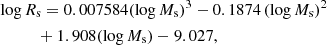
The Burstein et al. (1997) data. Over the years these very popular data have been examined by many authors, and therefore a detailed presentation is superfluous here. We limit ourselves to show in Fig. 1 the distribution on the log Rs versus log Ms plane of the various subgroups of the data set from the classical GCs to GCGs. The best fit of the ETGs with Ms ≥ 1010 M⊙ yields:

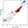 |
Fig. 1. log(Rs) vs. log(Ms) relation for all the samples under consideration. Rs is the half-mass radius and Ms the total stellar mass. Although Rs is not strictly identical to the effective radius Re, they are very close to each other. Throughout this paper we always use Rs, which is easier to calculate for hydrodynamic models of galaxies, and assume Rs ≃ Re. Burstein et al. (1997) sample: filled red circles are the ETGs, green open circles the SGs, blue filled triangles the DGs, filled red squares the GCs, and filled light-blue squares are the GCGs. The blue dashed line is the linear best fit of Eq. (2), i.e. log Rs = 0.60 log Ms − 5.859 relative to the sole ETGs, but extended to the regions of GCs and GCGs. Bernardi et al. (2010) sample: only ETGs are present, indicated by green filled circles. They fully overlap the ETGs of Burstein et al. (1997). The dashed magenta line is the linear best fit of the ETG data, but extended to GCs and GCGs. WINGS sample: dark-red filled circles are the ETGs, blue filled circles the BCGs, and the black filled circles are the GCGs. The olive-green dashed line is the linear best-fit of all WINGS objects together log Rs = 0.901log Ms − 9.245, but extended to DGs and GCs. Dwarf galaxies and Globular Clusters: coral filled circles are the DGs of Woo et al. (2008) and Geha et al. (2006) all together. Finally, the parallelogram shows the area occupied by the transition objects from GCs to DGs of Kissler-Patig et al. (2006). |
where Ms (in M⊙) is the star mass and Rs (in kpc) is the radius containing half of this mass (nearly identical to the classical effective radius Re). The scatter rms is 0.13 and the correlation parameter corr = 0.91. This relation is taken from Chiosi & Carraro (2002) who used the same data. This line is then extended to the domain of GCs and GCGs. Remarkably, the same MRR derived from the sole ETGs runs through the loci on the MR plane occupied by astrophysical objects whose mass extends over about 11 orders of magnitude (the blue dashed line). We feel that this cannot be a mere coincidence. Furthermore, this line splits the MR plane in two regions, one in which real objects can exist, and another one in which they cannot; see the analogous zone of avoidance in the kappa-space proposed by Burstein et al. (1997). Spurred by these arguments, we aim to cast light on the nature of the MRR.
The ETGs of Bernardi et al. (2010). A much richer sample of data for ETGs was derived by Bernardi et al. (2010) from the SDSS catalogue. The sample contains ≃60 000 galaxies2. The observational MRR is displayed in Fig. 1 by the green filled circles. These galaxies fully overlap with the ETGs by Burstein et al. (1997). The linear best fit of the SDSS data is

where Ms and Rs have their usual meaning and units, rms = 0.094, and the correlation parameter corr = 0.89. This MRR is shown in Fig. 1 by the magenta dashed line, and it is also extended to the regions of GCs and GCGs. The slope (and zero point) of the above MRR is quite robust as it nearly coincides with similar determinations made by other authors: e.g. Chiosi & Carraro (2002) using the Burstein et al. (1997) data and Shen et al. (2003) using the SDSS data.
The distribution of the bulk of galaxies is confirmed by the smaller sample of Shankar et al. (2013) also extracted from the SDSS survey but using slightly different selection criteria. The area covered by the observational data is slightly larger than the one with the Bernardi et al. (2010) data.
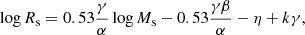
The WINGS database. In recent times, large optical and spectroscopic databases for the galaxy content of nearby clusters have become available thanks to the WIde-field Nearby Galaxy-cluster Survey (WINGS) of Fasano et al. (2006) and Varela et al. (2009) and the companion OMEGA-WINGS extension of Gullieuszik et al. (2015) and Moretti et al. (2017) for a number of clusters in the redshift interval (0.04 ≤ z ≤ 0.07). All this material has been subsequently examined by Cariddi et al. (2018) with particular attention paid to the problems of the accurate determination of the stellar light and the stellar mass profiles of galaxy clusters. WINGS measured and examined thousands of galaxies in 46 clusters, providing the absolute V and B magnitudes, the morphological types (according to the classification system RC3; de Vaucouleurs et al. 1991; Corwin et al. 1994; Fasano et al. 2012), four different estimates of the star formation rate (SFR), the star masses Ms (Fritz et al. 2007, 2011), the effective radii Re and effective surface brightness (D’Onofrio et al. 2014). The issue of the membership of the galaxies to the clusters under consideration was addressed and examined by Cava et al. (2009); we refer to this latter study for all details. In the present study, we consider all 46 clusters studied by Cariddi et al. (2018). The MR plane of this set of data is shown in Fig. 1 where the dark-red filled circles are the ETGs, the blue filled circles the BCGs, and the black filled circles the GCGs. The inspection of the WINGS data reveals that: (i) compared to Burstein et al. (1997) and Bernardi et al. (2010), at given mass the radii of ETGs are smaller by about 0.3 dex whereas those of BCGs and GCGs are comparable; (ii) the MRR relation for the ETGs more massive than 1010 M⊙ is

where masses and radii are in the usual units, rms = 0.22 and corr = 0.61; (iii) the scatter around this reference MRR is much greater than in the previous cases; (iv) ETGs and spiral galaxies crowd in the same region of the MR plane; (v) extended plumes at the large-mass side of the MRR may exist only for ETGs belonging to clusters and not for ETGs belonging to the field and in general not for both field and cluster late-type galaxies (D’Onofrio et al. 2019); and (vi) looking at the cluster ETGs, the MRR has a curved banana-like shape with a well developed plume toward high masses and radii made of red galaxies as confirmed by their B–V colour and also their Sérsic index n (D’Onofrio et al. 2019). In contrast, in field ETGs the banana-like structure of the MRR and the red plume are much less evident if at all. The reason for this striking difference is not clear, but it is most likely related to the higher probability for massive cluster ETGs to merge with and/or engulf other galaxies of smaller mass – in the case of wet mergers, thus avoiding any bluing effect in their colours – or of comparable mass and age – in case of dry mergers among similar objects, thus leaving the colour unchanged (see the discussion in Sciarratta et al. 2019).
Considering all the objects together (ETGs, BCGs and GCGs) the MMR is

with rms = 0.28 and corr = 0.95 (the dark olive-green dashed line in Fig. 1). It is worth noting that adopting Eq. (5) as the actual MRR for galaxies and galaxy clusters, one might conclude that the observed MRR simply mirrors the slope of 1 as expected from the virial equilibrium condition (D’Onofrio et al. 2019). In the present study we show that in reality the MRR originates from a more complicate interplay of different factors.
DGs. The DGs are taken from different sources: (i) the Burstein et al. (1997) sample of dEs and dSphs of the Local Group (indicated as B-DGs). It is worth recalling that the masses used by Burstein et al. (1997) are the dynamical masses and not the stellar masses, and so this group is not strictly homogeneous with the sample for ETGs; (ii) the sample of DGs by Geha et al. (2006; indicated as G-DGs); and (iii) the DGs of the Local Group according to the measurements made by Woo et al. (2008; indicated as W-DGs). Fortunately, all three samples of data yield similar MRRs:


Equation (6) is for the B-DGs with rms = 0.281 and corr = 0.632, Eq. (7) for the G-DGs with rms = 0.193 and corr = 0.300, and Eq. (8) for the W-DGs rms = 0.201 and corr = 0.851. Here we consider the three relationships as identical, but give more weight to that of Woo et al. (2008) with the highest correlation parameter. Finally, we take into account the study by Kissler-Patig et al. (2006) on the transition objects from GCs to dwarfs galaxies. All these data are shown in Fig. 1. In passing we note the much lower slope measured for DGs.
Galaxy clusters and groups. Two sources of data for galaxy clusters and groups have been considered, namely Burstein et al. (1997) and the WINGS and Omega-WINGS database (Fasano et al. 2006; Varela et al. 2009; Cava et al. 2009; Moretti et al. 2014; D’Onofrio et al. 2014; Gullieuszik et al. 2015; Moretti et al. 2017; Caminha et al. 2017; Cariddi et al. 2018). In particular the parameters Rs and Ms used in the present study are those measured by Caminha et al. (2017) and Cariddi et al. (2018). See also D’Onofrio et al. (2020) for more details.
The MRR slope. It is quickly evident that there is no unique slope for the MRR of ETGs and DGs. The slope for ETGs goes from 0.5 to 0.6, and for dwarf galaxies from 0.217 to 0.272. Furthermore, looking at the data in detail, the slope is even steeper than 0.54 in the region of the largest and most massive ETGs going up to 1 and even higher; see the top part of the MRR by Bernardi et al. (2010), Guo et al. (2009), van Dokkum et al. (2010), Graham et al. (2011, Fig. 1) and Graham (2013). This is a point to keep in mind when interpreting the observational data.
General remarks. Information and details on how the stellar masses Ms and half-mass radii, Rs, have been derived can be found in the original sources. Of course some possible systematic biases among the different sets of data are to be expected, although their effect ought to be small. This is somewhat supported by the overall agreement among different sources as far as some general relationships are concerned, such as for example the agreement in the slope of the MRR for ETGs between Bernardi et al. (2010) and Burstein et al. (1997). The same is true for the dwarf galaxies. However, since the groups of objects are treated separately here and only from a general qualitative point of view, no homogenisation of the data is needed. Furthermore, despite the important remarks about the WINGS galaxies, we can say that there is no substantial difference passing from the MRR based on the Burstein et al. (1997) data, to the one based on the Bernardi et al. (2010) data, and finally to that based on the WINGS data. Our analysis of the MRR for ETGs (and partially spirals as well) is primarily based on the SDSS sample of Bernardi et al. (2010), thus securing internal homogeneity of the mass and radius estimates. Finally, in the present study the MRR derived from the Bernardi et al. (2010) data is considered as a reference case.
3. Current theoretical models of galaxies and galaxy clusters
Our aim here is to present the numerical simulations of galaxies and clusters that we used to interpret and reproduce the observed properties of real galaxies and clusters. The primary source of data is the Illustris compilation3 (Vogelsberger et al. 2014a,b; Genel et al. 2014; Nelson et al. 2015, to whom we refer for all details), a suite of large, highly detailed cosmological hydrodynamical simulations, including star, galaxy, and black-hole formation tracking the expansion of the universe (Hinshaw et al. 2013). The procedure we adopted to extract theoretical data from the Illustris database is widely described in D’Onofrio et al. (2020). In order to follow the evolution of each galaxy, we extracted Illustris data for stellar mass, dark matter mass, total mass, luminosity, half-mass radius of the stellar component, velocity dispersion, and star formation rate for the whole set of galaxies (with mass log(Ms) ≥ 9 at z = 0) in the selected clusters at the redshifts z = 0, z = 0.2, z = 0.6, z = 1, z = 1.6, z = 2.2, z = 3, and z = 4. With these data we analysed the MRR at different epochs following the progenitors of each object.
In this section we present a quick analysis of the Illustris sample of galaxy models. Hereinafter MD, RD, MB, RB, Ms and Rs are masses and half-mass radii of dark matter (DM), baryonic matter (BM) made of stars and gas (initially only gas), and stellar mass (initially zero), respectively. The total mass of a galaxy is defined as MT = MD + MB. At the beginning, the ratio MD/MB = ω is fixed by the cosmological model of the Universe (in our case ω = 5.92 ≃ 6). It is worth keeping in mind that over the course of the formation and evolution processes, the above masses can change in the presence of galactic winds and/or stripping and/or acquisition of material by interactions with other galaxies or intergalactic medium.
3.1. Stars and DM: relationships among Ms, MD, Rs, and RD
The relationships Ms versus MD and Rs versus RD for four different redshifts (z = 4, 2, 1, and 0) are shown in the left and right panels of Fig. 2, respectively. Masses (in M⊙) and radii (kpc) are in logarithmic notation and the colour code indicates the redshift (z = 4, blue; z = 2, green; z = 1, yellow; z = 0, red).
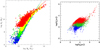 |
Fig. 2. Left panel: Ms − MD relations at different redshifts (z = 4, blue; z = 2, green; z = 1, yellow; z = 0, red). Masses are in solar units. The solid lines are the best fits, the coefficients of which are given in Table 1. Right panel: same as in the left panel but for the Rs − RD relations. Radii are in kiloparsecs. |
The Ms versus MD relationship. At the beginning of the galaxy formation history, DM and BM are in cosmological proportions (i.e. MD = ωMB with ω ≃ 6), but star formation gradually stores more and more baryonic mass into stars. It may be of interest to evaluate the efficiency of the star formation process over the Hubble time in galaxies of different mass. As MB < MD, Ms is always smaller than MD. However, because galaxies of different total mass may build stars at different efficiencies, the ratio Ms to MD is not expected to be constant, but to vary with MD and redshift. In the left panel of Fig. 2, we note that Ms always increases with MD, meaning that low-mass galaxies build up less stars with respect to the more massive ones. However the slope of the relation decreases as the redshift goes to zero. In more detail, for redshifts z ≳ 2 and masses MD ≃ 1012 M⊙ the slope decreases at decreasing redshift so that more and more stars are present at a given MD. More precisely, for z ≲ 2 and MD ≤ 1012 M⊙ the above trend holds true, but above this mass limit the opposite seems to occur: at a given MD less star mass is present than expected. In other words, massive galaxies are less efficient builders of their stellar content (the star formation is over). The relationship between log Ms and log MD is Ms = αMD + β and the best fits are given in Table 1.
Ms vs. MD and Rs vs. RD relations.
To quantify the star formation efficiency we calculate the ratio Ms/MD as a function of MD. In this case we can neglect the change of slope in the Ms-versus-MD relation above a certain value of MD at low redshifts. Finally we get the inverse of Ms/MD given by the expression
where the ratio MB/Ms measures how much of the original BM mass is turned into stars.
The values of (1 − α) and −β are listed in Table 2 for the four redshifts we are considering.
Coefficients of the relationships log(MD/Ms) = (1−α) log MD − β at different redshifts.
For the sake of illustration, in Table 3 we list the ratio Ms/MD as a function of the total mass limited to the case of z = 0. In general, the ratio Ms/MD increases with decreasing total galaxy mass. Similar results were found by Chiosi & Carraro (2002), Merlin & Chiosi (2006, 2007), and Merlin et al. (2012), showing that old models were already able to catch the basic aspects of the galaxy formation problem.
Efficiency of the star formation in galaxies of different mass observed at redshift z = 0.
The Rs vs. RD relationship. In a similar way, we derive the relations  which are shown in the right panel of Fig. 2 and the entries of Table 1 for the case of z = 0. The radius of RD is more extended than Rs by a factor between ∼3 and 10 as the galaxy mass increases from 109 M⊙ to 1013 M⊙. The slope γ of the Rs − RD relation (logarithmic) first decreases by about a factor of two passing from z = 4 to z = 1, and then increases again at z = 0. What is more important is that while at high redshifts (our z = 4, z = 2 and z = 1 cases) the galaxy distribution on the Rs versus RD plane is a random cloud of points, at z = 0 a regular trend appears in which Rs increases with RD when this latter tends to larger values (larger masses). Towards low values of both radii and masses, a cloud of points is still there. The effect of this is to increase the mean slope of the whole distribution. Below, we try to cast light on the implications of this latter finding.
3.2. The Rs vs. Ms relation at different redshifts
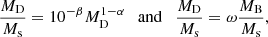
Figure 3 shows the Rs-versus-Ms relations of the Illustris models at the four redshift values considered here. As in the case of Rs versus RD, the distribution is clumpy and irregular at high redshifts independently of the galaxy mass. Starting from z = 1, and more evident at z = 0, a tail-like feature develops towards large masses (≳1−2 × 10¹¹ M⊙).
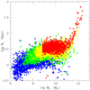 |
Fig. 3. Stellar half-mass radius Rs vs. mass Ms of the galaxy models of the Illustris database at different redshifts: z = 4 (blue), z = 2 (green), z = 1 (yellow), and z = 0 (red). |
The best fit of the data at redshift z = 0 using the relationship  (where mass and radius are in M⊙ and kiloparsecs, respectively) yields the values listed in Table 4. At higher redshifts, the tail at the side of large masses is much less evident if not missing at all. The tail seems to disappear starting from z = 1. The Rs-versus-Ms relation is similar to that for the low-mass galaxies at z = 0, that is, almost flat. At any value of mass in the mass range of the data cloud, the dispersion in the radius is very large. At redshift z = 0, the tail has a very similar slope and zero point to those derived by Chiosi et al. (2012) using the SDSS data of Bernardi et al. (2010).
Radius–mass relation of the stellar component  .
.
What is the reason for the cloud-like and tail-like distributions at low redshifts? Why does the cloud-like distribution dominate in the low-mass range and at high redshifts? The opposite trend is seen for the tail-like distribution, which shows up in the high-mass range and at low redshifts. To cast light on the physical meaning of these two distributions, we examine the history of the Rs-versus-Ms relation of a number of individual galaxies.
3.3. The detailed history of the Rs-versus-Ms relation for selected models
The Illustris simulations are based on the hierarchical scheme, and therefore each galaxy is the result of a number of mass acquisition and/or removal processes, which change the masses MD and Ms and the radii RD and Rs of the galaxy. For each galaxy in the sample at z = 0, the Illustris database provides the past history, that is, the masses and radii of the component sub-units during the Hubble time. This means that we can reconstruct the past history in the Rs-versus-Ms plane of each galaxy from z = 4 to z = 0. Figure 4 shows the path on the MR plane of 20 cases randomly chosen from the whole sample. The path followed by each galaxy is quite tortuous. We can summarise the complex situation as follows. In mergers between low-mass objects, the mass and the radius increase, but exceptions are possible, where either the mass or the radius or both decrease. In general, the model galaxies remain inside the cloud-like region of the Rs-versus-Ms plane. Mergers among galaxies of relatively high mass tend to generate objects that shift outside the cloud and tend to fall close to a well-behaved radius–mass sequence (they indeed define it) and their locus agrees with the observational radius–mass relationship for ETGs (see e.g. Chiosi et al. 2012, and references therein). Finally, the cloud-like region roughly coincides with the distribution of DGs of different types (see the discussion by Chiosi & Carraro 2002). The MRR for massive galaxies is very close to the relation set by the condition of virial equilibrium (this issue is examined in great detail below), so one might be tempted to conclude that systems that at the present time (z = 0) are able to satisfy the virial condition have the minimum energy and hence radius for their existing structure. DGs cannot be in this ideal condition, most likely because they are undergoing active star formation. Therefore, the question arises spontaneously as to whether or not there are DGs that fulfill the virial state. Also, what determines the large radius of DGs? (see Fig. 1.) In other words, are there DGs whose position on the MR plane is near the MRR of normal ETGs? Can DGs be in conditions of mechanical and thermal equilibrium? The following considerations can be made.
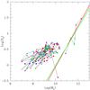 |
Fig. 4. Evolution of Illustris galaxies on the Rs versus Ms plane from z = 4 to z = 0. There are eight values of redshift along each line. The position of each galaxy at each redshift is marked by a point of different colour. The colour code is as follows: blue (z = 4.0), medium-blue (z = 3.0), light-green (z = 2.2), green (z = 1.6), cyan (z = 1.0), magenta (z = 0.6), coral (z = 0.2), and red (z = 0). The solid lines are the best fits of the Illustris data for z = 0 in the domain of massive galaxies MT ≥ 1011 M⊙ (red), and of the Bernardi et al. (2010) ETGs by Chiosi et al. (2012; green). Here we show 20 cases randomly chosen from the whole sample. |
Given the mass of a galaxy (either acquired by mergers or already in place “ab initio”), the radius mirrors the condition of mechanical equilibrium of the system; in other words, it is a consequence of the energy balance between the dynamical collapse and feedback by star formation and other sources. To answer the above questions, we look to galaxies in which (at least) star formation activity was extinguished a reasonable amount of time ago. To this aim, we consider the z = 0 sample and isolate the galaxies with zero star formation rate (SFR = 0) or the minimum value in the sample, namely 10−4 M⊙ yr−1 (see Fig. 5). In addition to galaxies of high mass, there are also a few objects of low mass that fall very close to the prolongation of the best-fit line of the Bernardi et al. (2010) ETGs (see Chiosi et al. 2012). Their observational counterparts could be objects like ωCen and M32. It seems that also low-mass galaxies can exist that share the same equilibrium conditions as the massive ones. However, this conclusion is biased by the large uncertainties on the SFR, which is known only up to three decimal places. A SFR of the order of 10−4 M⊙ yr−1 or lower cannot be neglected in the case of dwarf galaxies. This may explain why even for this case a residual cloud-like feature still remains.
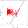 |
Fig. 5. Same as Fig. 3 but limited to the sample for z = 0 for all models with zero star formation rate. |
3.4. Comparison between observations and theory
Before proceeding further, it is mandatory to compare the observational data with the theoretical galaxy models in use. This is shown in Fig. 6, which displays the following data: (i) the fairly homogeneous sample of GCs, DGs, ETGs, and GCGs by Burstein et al. (1997); (ii) the Bernardi et al. (2010) sample of ETGs, which is by far richer than the previous one for galaxies of the same type; and (iii) the WINGS data for ETGs, BCGs, and GCGs by Valentinuzzi et al. (2011) and Cariddi et al. (2018). The main focus is on the group of ETGs. The theoretical models are those of the hydrodynamical large-scale simulations of the Illustris project by Vogelsberger et al. (2014a,b) at redshift z = 0 (the olive green dots) in the pure hierarchical scheme, the models of (Chiosi & Carraro 2002) in the pure monolithic scenario, and finally those by Merlin & Chiosi (2006, 2007), Merlin et al. (2010, 2012), Chiosi et al. (2012) in the so-called early-hierarchical view, both at redshift z = 0. The emphasis here is on the Illustris models, which are considered as the reference case. From this comparison, we make the following observations: (i) The Burstein et al. (1997) data for ETGs agree relatively well with the Illustris models of comparable mass. Unfortunately Illustris does not sufficiently cover the regions populated by DGs, simply because for technical reasons the sample at z = 0 is limited in mass at 109 M⊙. In addition, the observational sample at disposal does not contains enough DGs. Therefore, nothing can be said for this type of object. As already noted, the MRR of ETGs given by Eq. (2) has a slope ≊0.6, even though the most massive ETGs would be better represented by a slope ≃1, which suggests an MRR whose slope slowly changes with increasing mass. We return to this point below. This best-fit-line for ETGs, extended downward to the domain of GCs, upward to that of GCGs, and vertically shifted upwards by Δlog Rs ≃ 0.3, would match all three groups of objects and leave all the data in the semi-plane above it.
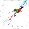 |
Fig. 6. Composite Rs-versus-Ms relation and comparison between theory and observations. The light powder-blue dots are the data of Burstein et al. (1997) for ETGs, DGs, GCs, and GCGs, and the dashed line of the same colour is the best fit of the sole ETGs, this time extended to the domains of GCs and GCGs. The bright green dots are the Bernardi et al. (2010) data for ETGs, and the thick dashed line of the same colour is the best-fit line of these latter. The red, blue, and green-blue dots are the ETGs, BCGs, and GCGs of the WINGS sample. The dashed red line is the best-fit line of the ETGs, whereas the solid blue line is the best fit of all WINGS data lumped together. The slope of this latter line is very close to the MRR for virialised objects. In this case the line fails to hit the region of GCs. Finally, we display different theoretical models for comparison. The black filled squares connected by the black solid line and the red squares connected by the solid red line are the monolithic models by Chiosi & Carraro (2002) and their linear fit. The two groups of models differ for the density of the Universe (redshift) at initial collapse. The three coral open circles are low-mass ETGs with the same mass but slightly different initial densities by Chiosi & Carraro (2002); see the data of Table B.2. The empty red star is the merger reported by Chiosi & Carraro (2002). The blue squares connected by the blue line are the hierarchical models by Merlin et al. (2010, 2012); see Table B.3 for more details. The light blue-green squares are the ancillary model of Chiosi et al. (2012); see Table B.3. Finally, the dark olive-green points are the reference model galaxies of the Illustris simulations. |
(ii) The same results and considerations hold true for the Bernardi et al. (2010) data, for which the best-fit MRR of the ETGs is given by Eq. (3), which is only slightly different from the previous one. The fit agrees with that of Burstein et al. (1997) and with the Illustris models. The extension of the MRR for ETGs also hits the GCs and GCGs.
(iii) The WINGS data all together suggest a steeper slope of the MRR, namely 0.95 ± 0.02. The inclusion of galaxy clusters has forced the slope to higher values. Extending this relation (the solid line) to the domain of GCs would not match these objects. Furthermore, the WINGS data do not cover the region of galaxies with Ms ≃ 109 M⊙ meaning that they do not completely overlap the area reached by Illustris models. However, if we derive the MRR limited to the case of ETGs, the agreement between theory (Illustris) and data is remarkable and the best-fit line of the ETGs alone (long-dashed line) would hit the region of GCs.
The main conclusion of this mutual comparison between data from different sources and the theoretical models of Illustris is that all of them seem to agree with each other relatively well. As a matter of fact, different sources of observational data, different photometry, and different volume coverage of the space lead to similar results. This is very important because it suggests that our analysis does not severely depend on the source of data.
Finally, we proceed to compare our theoretical models with other theoretical models. This is shown in Fig. 6. The black filled squares connected by the black line are the models by Chiosi & Carraro (2002) for low initial over-density with respect to the surrounding medium and different mass, whereas the red squares connected by the red line are models of the same type but different mass and very high initial over-density contrast. The three coral circles are monolithic models of the same mass (109 M⊙) but different initial density contrast by Chiosi & Carraro (2002). The blue filled squares connected by the blue line are the models by Merlin et al. (2010, 2012). The light blue-green filled squares are incomplete models of different mass and initial over-density limited to the very first evolutionary stages calculated by Chiosi et al. (2012) according to the early hierarchical scheme. These latter are meant to localise the initial position of model galaxies on the MR plane. Details on the input and output parameters of all the model galaxies are given in Tables B.1–B.3. It is worth noting that the slope of the MRR of the models at varying mass but constant initial conditions (over-density) are very similar one another.
Remarkably, there is substantial agreement among the various types of models. Taking the Illustris case as a reference, the monolithic and early hierarchical models fall onto the same position on the MR plane, the only difference being due to the richness of the three samples. While the Illustris models amount to more than 2500 cases of different mass (total and stellar) and initial conditions that are picked up from large-scale simulations (see Vogelsberger et al. 2014a,b, for more details), those by Chiosi & Carraro (2002) and Merlin & Chiosi (2006, 2007), Merlin et al. (2010, 2012), Chiosi et al. (2012) are much fewer in number and the initial conditions are alternatively defined. The Chiosi & Carraro (2002) models were designed and calculated one by one assuming the initial over-density of the proto-cloud with respect to the surrounding cosmological medium and the initial positions and velocities of the DM and BM particles. Those by Merlin & Chiosi (2006, 2007), Merlin et al. (2010, 2012), Chiosi et al. (2012) stem from mini large-scale numerical cosmological simulations (about 10 Mpc by 10 Mpc) that allowed for repeated mergers among sub-clumps of DM and BM in the same field. In this respect they are somewhat similar to the models by Vogelsberger et al. (2014a,b).
From this comparison, we also learn some important facts: (i) At a given total star mass Ms at the present time (z = 0), galaxies tend to have the same size Rs independently of their past formation history (pure monolithic, early hierarchical, pure hierarchical) because they all share the same area of the MR plane. (ii) Furthermore, hydrodynamic simulations of galaxies that share more or less the same initial conditions tend to converge to the same MRR regardless of the details of the input physics and numerical technique. The MRRs of models with different initial conditions tend to be parallel to one another on the MR plane. Objects of higher initial density of the same total star mass tend to remain smaller in size throughout their entire lifetime. (iii) The MRRs predicted by models are always flatter than the observed ones by approximately a factor of two. (iv) Models calculated with modest computing resources, simplified physical input, and numerical technique are fully adequate to explore a large variety of astrophysical problems.
The most important issues and questions raised by the results of this section are as follows: (1) Can the MRR of ETGs be considered to be of more general significance and be extended to encompass a much wider range of astrophysical objects going from GCs to GCGs? (2) If so, what is the physical meaning of this line splitting the MR plane in two regions: (a) the region containing objects with mass spanning about ten orders of magnitude from GCs to GCGs; and (b) the region void of objects with the exception of the much fewer compact galaxies (see Chiosi et al. 2012, for a short discussion on this issue). (3) The fact that the separation seems to be very sharp. (4) In principle, galaxies of suitable mass and/or initial density could fall in the “forbidden semi-plane” but for some yet unknown reason the vast majority of real galaxies do not. It is worth recalling that the forbidden semi-plane coincides with the region named the “zone of exclusion (ZOE)” by Burstein et al. (1997). A plausible explanation of the “forbidden semiplane” was put forward long ago by Chiosi & Carraro (2002) and Chiosi et al. (2012); considering the recent wealth of modern data and theoretical models, we revisit this explanation in the following.
4. Theoretical predictions for the MRR
In this section, we examine the theoretical foundations of the MRR of galaxies and highlight the possible physical causes of its occurrence. First, we look for a simple explanation for the slope of the theoretical MRR. Second, from large-scale simulations of the cosmological number density distributions of DM halos as a function of redshift we derive the MRR of halos at z = 0, and with the aid of this MRR we derive the present-day MRR of their star content, that is, the observational MRR of galaxies.
4.1. The MRR of collapsing proto-galaxies made of DM + BM
We start looking for a simple explanation of the MRR of galaxy models whose slope is lower than the observational one by approximately a factor of two. Independently of the formation scheme (either monolithic or hierarchical), the seeds of galaxy structures are perturbations of matter made of DM and BM that undergo collapse when the density contrast with respect to the surrounding medium reaches a suitable value. Assuming spherical symmetry for the sake of simplicity, indicating the total mass and associated radius with MT and RT, and making the approximation MT = MD + MB ≃ MD and RT ≃ RD, we may write the MRR for individual galaxies as
where ρu(z) ∝ (1 + z)3 is the density of the Universe at the redshift z, and λ is the factor for the density contrast of the DM halo. This expression is of general validity, whereas the function λ depends on the cosmological model of the Universe, including the ΛCDM case. All details and a demonstration of this expression can be found in Bryan & Norman (1998) and their Eq. (6).
The collapse will increase the mean density of DM and BM, meaning that when a critical value of the BM density is reached, stars can form and an object made of stars grows at the centre of the system according to its star formation rate. Therefore, we expect a new MRR to develop for the BM component turned into stars, of type

In the context of the ΛCDM cosmology, Fan et al. (2010) adapted the general relation of Eqs. (10) and (11) to provide an expression linking the halo mass MD and the star mass Ms of the galaxy born inside it, the half light (mass) radius Rs of the stellar component, the redshift at which the collapse takes place zf, the shape of the BM galaxy via a coefficient Ss(ns) related to the Sersic brightness profile from which the half-light radius is inferred, the Sersic index ns, the velocity dispersion of the BM component with respect to that of DM (expressed by the parameter fσ), and finally the ratio m = MD/Ms. The expression is
A typical value for the coefficient Ss(ns) is 0.34. Furthermore, fσ yields the three-dimensional star velocity dispersion as a function of the DM velocity dispersion, σs = fσσD. Here we adopt fσ = 1. For more details, see Fan et al. (2010) and references therein.
The most important parameter of Eq. (12) is the ratio m = MD/Ms. Using the Illustris data we investigated how this ratio varies in the mass interval 108.5 < MD < 1013.5 (masses are in M⊙) and from z = 0 to z = 4, and made some predictions over a wider mass range 104 < MD < 1015 and a wider redshift interval from z = 0 to z = 10. The analysis and results are presented in Appendix A where we confine m(MD, z) within a rather narrow range of possible values and suggest that a simple relationship giving the ratio m as a function of MD might be the one of Eq. (A.5), which we repeat here for the sake of clarity:
This relation turns out to be sufficiently accurate for the qualitative nature of our investigation. In a very recent study, Girelli et al. (2020) thoroughly investigated the stellar-to-halo mass ratio of galaxies (Ms/MD = 1/m i.e. the inverse of our parameter m) in the mass interval 1011 < MD < 1015 and redshifts from z = 0 to z = 4. They used a statistical approach to link the observed galaxy stellar mass function on the COSMOS field to the halo mass function from the ΛCDM–dust grain simulations and an empirical model to describe the variation of the stellar-to-halo mass ratio as a function of redshift. Finally, these latter authors provide analytical expressions for the function m(MD, z). Noting that in the mass interval in common, their results are in substantial agreement with those inferred from the Illustris data, we prefer to provisionally adopt here Eq. (A.5) for the sake of internal consistency with the theoretical galaxy models used here.
We would like to point out that Eq. (12) is strictly valid only for monolithic infall of BM into collapsing DM potential wells. Nevertheless, this formula provides a general reference with which to obtain the typical dimension of a galactic system as a function of its mass and formation redshift. While adjustments are possible, the general trend is well defined. However, some deviations from this law are possible and expected, for example for low redshifts; see below for further discussion. The MR plane of the hydrodynamic models and the loci expected for different redshifts from Eq. (12) are shown in Fig. 7 together with the ETGs by Bernardi et al. (2010).
 |
Fig. 7. Comparison of the Fan et al. (2010) lines and the theoretical models by Merlin et al. (2012; green filled squares) with the observational data of Burstein et al. (1997) from GCs (small red squares), to DGs (small blue triangles), and GCGs (light blue filled circles) plus the ETGs of Bernardi et al. (2010; red dots). The short-dashed blue line is the Fan et al. (2010) relation for z = 0. The thin solid lines of different colours are the same relation but for z = 1, z = 5, z = 10, z = 15, and z = 20 from top to bottom in the order. The long-dashed, thick blue line is the best-fit of the ETGs of Bernardi et al. (2010) extended to GCs and GCGs. |
The slope of Eq. (12) is almost identical to the one estimated from the hydrodynamic models; the small difference can be fully ascribed to the complex baryon physics, which causes the stellar system to be slightly offset with respect to the locus analytically predicted from DM halos. Therefore, a model slope (close to 1/3) different from that of the observational MRR is not the result of inaccurate description of the physical processes taking place in a galaxy; on the contrary, it mirrors the fundamental relationship between mass and radius in any system of given mean density. Indeed it is remarkable that quite complicated numerical calculations clearly display this fundamental feature. If this is the case, why do real galaxies gather along a line with a different slope?
What is still missing in the above MRR is that galaxies (globular clusters and cluster of galaxies) form and evolve in a given cosmological scenario which ultimately drives the demography of objects over a large range of masses and dimensions in any given volume of arbitrary size of the Universe. In other words, the real MRR is given by the convolution of the MRR of each component with the underlying cosmological scenario that determines the mass interval spanned by galaxies at each redshift and the relative percentage of galaxies of a certain mass with respect to the others (otherwise known as halo mass function).
4.2. The MRR from the DM halo growth function n(MD, z)
The similarity of the MRR passing from star clusters to single galaxies of different mass and morphological type and eventually to galaxy clusters suggests that a profound relationship exists between the way all these objects populate the MR plane and the cosmological growth of DM halos.
The distribution of the DM halo masses and their relative number density as a function of redshift have been the target of numerous studies. These works culminated in large-scale simulations of the structure of the Universe, such as for example the Millennium simulation (Springel et al. 2005). In parallel, many studies investigated the so-called halo growth function (HGF) as the integral of the halo mass function (HMF). Among others (see e.g. Angulo et al. 2012; Behroozi et al. 2013) we recall and make use of the results by Lukić et al. (2007) who, using the ΛCDM cosmological scenario and the HMF of Warren et al. (2006), derive the HGF n(MD, z). This gives the number density of halos of different masses per (Mpc h−1)3 resulting from all creation and/or destruction events. The growth function is expressed in terms of the normalised Hubble constant h = H0/100, where H0 is assumed to be H0 = 0.1 km s−1 Mpc−1. The explored interval of redshift goes from 0 to 20. The n(MD, z) function of Lukić et al. (2007) is shown in Fig. 84. Similar HGFs have been investigated, for example those by Angulo et al. (2012) Behroozi et al. (2013). For more details, see Chiosi et al. (2012).
 |
Fig. 8. Growth function of halos n(MD, z) reproduced from Lukić et al. (2007). |
The analytical representation of the n(MD, z) function displayed in Fig. 8 is given by
where the coefficients An(MD) are listed in Table 5. We then count the total number of halos per mass bin Δlog MD at redshift z = 0. This is simply given by reading off the values of the curves along the y-axis and interpolating for intermediate values. These are the halos that would nowadays populate the synthetic-MR plane and that should generate the observed galaxies. Since the total number of halos drawn from the Lukić et al. (2007) plot refers to a volume of 1 (Mpc h−1)3, any meaningful comparison with observational data requires a suitable scaling of the theoretical values by a suitable factor to match the real volume of the observed portion of the sky from which the data are obtained (see below).
Although the following points, (i) to (iii), are well known – see the pioneer studies by Press & Schechter (1974) and Lukić et al. (2007, see for ample referencing), for the sake of clarity and as relevant to our discussion, we note the following: (i) for each halo mass (or mass interval) the number density is small at high redshift, increases to high values towards the present, and depending on the halo mass either takes a maximum value at a certain redshift followed by a decrease (typical of low mass halos) or keeps increasing as in the case of high-mass halos. In other words, the first creation of halos of a given mass (by spontaneous growth or perturbation to the collapse regime) overwhelms their destruction (by mergers), whereas the opposite occurs for low-mass halos past a certain redshift; (ii) at any redshift, high-mass halos are orders of magnitude less frequent than low-mass ones; and (iii) at any redshift, the mass distribution of halos has a typical interval of existence, the upper mass end (cut-off mass) of which increases at decreasing redshift. Given a certain number density of halos Ns, on the n(MD, z) − z plane of Fig. 8 this would correspond to a horizontal line intersecting the curves for the various masses at different redshifts, that is, obeying the equation n(MD, z) = Ns. Each intersection provides a pair (MD, z) which gives the mass of the halos fulfilling the condition Ns = n(MD, z) at the corresponding redshift z (or vice versa, the redshift satisfying the condition for each halo mass). For any value Ns we get an array of pairs (MD, z) that can be extrapolated to a continuous function that, with the aid of the Fan et al. (2010) relationship (in which the parameters m and fσ are fixed), provides the corresponding relationship between the mass in stars and the half-mass radius of the baryonic galaxy associated to a generic host halo to be plotted on the MR plane.
Repeating the procedure for different values of Ns, we get a manifold of curves on the MR plane. It turns out that with the Ns corresponding to 10−2 halos per (Mpc h−1)3 (which roughly corresponds to the volume surveyed by the SDSS), the curve is just at the edge of the observed distribution of ETGs on the MR plane. Higher values of Ns would shift the curve to larger halos (baryonic galaxies); the opposite is true for lower values of Ns. What is remarkable about Ns = 10−2 halos per (Mpc h−1)3 ? Based on crude and simple arguments, we recall that the total number of galaxies observed by the SDSS amounts to about ≃106, whereas the volume of the Universe covered by it is about a quarter of the whole sky multiplied by a depth of ≃1.5 × 10⁹ light years, that is, ≃108 Mpc3, to which the number density of about 10−2 halos per (Mpc h−1)3 would correspond5.
It is worth noting here that Ns is not a free parameter. Its value is indeed determined by the sample of observational data under examination. In other words, Ns translates the theoretical relative number densities of halos per 1(Mpc h−1)3 into the real number density of the observational data. In this study we fix Ns on the richest sample of ETGs at our disposal, that is, that of Bernardi et al. (2010).
The equation n(MD, z) = Ns with Ns = 10−2 or equivalently 106 halos per 108 Mpc3 recast to derive the halo mass MD as a function of z becomes

from which we get MD. With the aid of Eq. (A.5) we derive the quantity m and from its definition we obtain Ms = MD/m. Finally, from Eq. (12) we derive the associated radius Rs.
The analytical fit of the MR relation determined in this way and limited to the mass interval 9.5 ≤ log Ms ≤ 12.5 (Ms in solar units) is
This relation is meant to fit the distribution of only ETGs on the MR plane. We note that the slope gradually changes from 0.5 to 1 as we move from the low-mass to the high-mass range. It is worth recalling here that a similar trend for the slope is also indicated by the observational data (see van Dokkum et al. 2010, and references therein). Owing to the many uncertainties, we do not try to formally fit the median of the empirical MRR, but we limit ourselves to show that the locus predicted by Ns = 10−2 halos per (Mpc h−1)3 falls on the MR plane close to the observational MRR. Lower or higher values of the halo number density would predict loci in the MR plane that are too far from the observational MRR.
Finally, we highlight the fact that the locus on the MR plane defined by relation (16) is ultimately related to the top end of the mass scale of halos (and their associated baryonic objects) that can exist at each redshift. In other words, recalling that the mass of any intersection pair for Ns = 10−2 corresponds to halos becoming statistically significant in number on the observed spatial scale at the associated redshift, this can be interpreted as the so-called cut-off mass in the Press & Schechter (1974) or equivalent formalism (see Lukić et al. 2007, for details and references). Therefore, this also provides an upper boundary to the mass of galaxies that are allowed to be in place (to collapse) at each redshift. We name this locus the cosmic galaxy shepherd. All this is shown in Fig. 9, where we also plot the curves relative to Ns = 10−8 halos per (Mpc h−1)3, corresponding to 1 halo per 108 (Mpc h−1)3, for the sake of comparison.
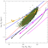 |
Fig. 9. Cosmic galaxy shepherd and the corresponding locus of DM parent halos (the black solid thick and thin lines, respectively) for the number density of Ns = 10−2 halos per (Mpc h−1)3. In addition to this we show the case with Ns = 10−8 halos per (Mpc h−1)3 (the magenta solid thick and thin lines). The various loci are plotted onto the observational MR plane (see text for all details). We also draw the observational data for the sample of Bernardi et al. (2010) with the linear fit obtained by these latter authors, and two theoretical MRRs from Eq. (12) of (Fan et al. 2010; solid thin blue lines) relative to z = 0 and z = 10, with m = 15 and fσ = 1. In addition to this, the present-day position of the reference galaxy models and their linear fit are shown (the golden filled squares and solid line). Finally, the filled black squares and magenta circles show the cosmic galaxy shepherd at different redshifts (z = 0, 1, 5 10, 15, and 20) for the two cases of the number density per (Mpc h−1)3. |
There are two points to be clarified. First, this way of proceeding implies that each halo hosts one and only one galaxy and that this galaxy is an early-type object matching the selection criteria of the Bernardi et al. (2010) sample. In reality ETGs are often seen in clusters and/or groups of galaxies and many large spirals are present. Only a fraction of the total population are ETGs. One could try to correct for this issue by introducing some empirical statistics about the percentage of ETGs among all types of galaxies. Despite these considerations, to keep the problem simple we ignore all this and maintain the minimal assumption that each DM halo hosts at least one baryonic component made of stars. This is a strong assumption, and a subject to which we return below. Second, we assume that m varies with halo mass. According to Fan et al. (2010), the empirical estimate of the MD/Ms ratio is about 20–40. Our estimate yields a mean value of ⟨m⟩≃20. However, a slightly higher value for m does not invalidate our analysis, because it would simply shift the location of the baryonic component on the MR plane corresponding to a given value of Ns. Finally, fσ = 1 is a conservative choice. The same considerations made for m also apply to this parameter.
Along the line for the cosmic galaxy shepherd, redshift and cut-off mass go in inverse order, that is low masses (and hence small radii) at high redshift and vice versa. This means that a manifold of MRRs defined by Eq. (12), each of which referring to a different collapse redshift, can be selected, and along each MRR only masses (both parent MD and daughter Ms) smaller than the top end are permitted, each of them with a different occurrence probability: low-mass halos are always more common than high-mass ones. In the observational data, it looks as if ETGs should occur only towards the high-mass end of each MRR, that is, along the locus on the MR plane whose right hand side is limited by the cosmic galaxy shepherd. This could be the result of selection effects, that is, (i) galaxies appear as ETGs only in a certain interval of mass and dimension and outside this interval they appear as objects of different types (spirals, irregulars, dwarfs, etc.), or (ii) they cannot even form or be detected (e.g. very extended objects of moderate/low mass). Finally, in addition to this, we argue that another physical phenomenon also limits the domain of galaxy occurrence on the side of the small, low-mass objects. We return to this phenomenon below.
4.3. More on the cosmic galaxy shepherd
If we compare the present-day position of the reference hydrodynamical models on the MR plane with the region populated by real galaxies (see Fig. 6 and/or Fig. 7), at first glance one would be tempted to conclude that only the high-mass models suited to massive ETGs agree well with observations, whereas the low-mass ones (and to some extent also those of intermediate mass) apparently have overly large radii with respect to their masses. However, before concluding that the models fail to reproduce the data, it is worth recalling that the observational distribution of galaxies on the MR plane results from the combined action of many factors not yet taken into account by our analysis. Is the observational sequence of ETGs populated only by galaxies behaving as our massive ones or are there others with different behavior? Since for any value of the halo mass there is a certain redshift below which halos of this mass start decreasing in number by mergers (Lukić et al. 2007), galaxies generated by those halos become increasingly unlikely, as should be the case for our low-mass models. Indeed, when at a given redshift we have assumed the existence of halos of any mass, we have neglected this important effect. Therefore, the situation may occur that halos/baryonic model galaxies are calculated and plotted onto the MR plane even though according to the above arguments their existence is very unlikely.
On these grounds, we argue that the observational MRR of ETGs (galaxies in general) is the result of two factors: the halo growth function providing the number density of halos of different mass as a function of redshift (in the concordance ΛCDM Universe), and the fundamental MRR determining the probable size of a galaxy as a function of its mass and formation redshift after collapse.
5. Improving constraints in the cosmological context
In this section we seek a common explanation for the observational distribution of astronomical objects, going from GCs, to galaxies like DGs and ETGs (and to a less extent also spiral galaxies), to clusters of galaxies, the mass of which spans about 11 orders of magnitude. The situation is shown in Fig. 10. The pale-blue filled circles are the normal, giant ETGs, the DGs, the GCs, and the GCGs. No distinction is made between different groups or sources of data. The aim here is to qualitatively display the region of the MR plane populated by real objects of different mass, size, and morphological type.
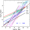 |
Fig. 10. Mass-radius relationship: comparison between data and theory. Radii Rs and stellar masses Ms are in kiloparsecs and M⊙, respectively. The pale-blue filled circles are all the data considered in this study, and the pale green filled circles are the models of Illustris. The dark-red thick crossed line is the linear best fit of normal ETGs (MT ≥ 1010 M⊙) given by Eq. (3), but prolonged down to the region of GCs and upwards to that of GCGs. The four solid dashed line labelled Mod-A (zf = 5, blue), Mod-B (zf = 1, red and zf = 2, dark green), and Mod-C (zf = 10 black) are the analytical relationships of Eq. (34) showing the loci of galaxy models with different mass but constant initial density for different values of redshift of galaxy formation zf as indicated. These lines are the best fit of the models by Chiosi & Carraro (2002), Merlin et al. (2012), and Chiosi et al. (2012); see Tables B.1–B.3. The magenta solid lines show the virial condition on the MR plane for different velocity dispersion (50, 250 500 km s−1 from left to right). The dashed black lines labeled by different values of zf are the MRRs expected for galaxies with total mass equal to 50 × MCO(z), the cut-off mass of the Press-Schechter at varying zf according to relation (35). These lines go in pairs with the best-fit lines of models of identical initial density labelled with the same colour. The large empty squares illustrate the intersections between the lines of constant initial density and the MRRs for 50 × Mco galaxies for equal redshift. All the intersections lie very close to the relation of Eq. (3) shown by the dark-red crossed line. This is the linear interpretation of the observed MRR, i.e. the analytical demonstration of Sect. 5. Finally, the curved blue dotted line shows the expected MRR for the baryonic component of DM halos whose mass distribution follows the cosmological HGF by Lukić et al. (2007). The curve has been extended to include the GCs and the GCGs (see main text for more details). We highlight the ever changing slope of the MRR which decreases passing from GCGs to ETGS and GCs. Remarkably, the curved line first runs very close to the large empty squares, and then secondly to a linear fit of the data (crossed line), and third accounts for the observed MRR passing from GCs to GCGs (about ten orders of magnitude difference in star mass). The horizontal blue line shows the interval for Ms corresponding to initial masses MCO(z) < MT < 10 × MCO(z) (the percentage of galaxies in this interval amounts to ≃15%), which highlights the fact that at each redshift the high-mass edge of the MRR has a natural width. |
5.1. The observational situation: evidence of a unique MRR
Let us quickly summarise once more the main features of the distribution of astrophysical objects of different types on the MR plane. (i) The family of GCs is well detached from the body of normal, giant ETGs (let us say those with mass larger than about 1010 M⊙). However, the region in between is populated by DGs. At the top of the distribution there are the GCGs with the largest radii and masses. The richest sample at our disposal is made of ETGs (the spiral galaxies occupy more or less the same region). The relative number of objects per group is not indicative of the real number frequencies because severe selection effects are present. The best fit of the ETG data from the various sources yields the relations of Eq. (2) for Burstein et al. (1997), Eq. (3) for Bernardi et al. (2010), and Eq. (4) for the WINGS data, in which only objects with Ms ≥ 1010 M⊙ are considered not to contaminate the samples with DGs. Since the slopes differ by 0.1 and the zero-points by 0.88, we consider the three relationships to be fully equivalent. (ii) If we extrapolate any of the relation above, which holds for massive ETGs downward to the mass range of GCs and upward to that of GCGs, we see that the same relation provides a lower limit to GCs, passes through ωCen and M32, provides the lowest limit to the distribution of DGs, and finally reaches the region of GCGs. (iii) There are no galaxies in the semi-plane for radii Rs smaller than the values fixed by relation (3), independently of the galaxy mass, but for the so-called “compact galaxies” that we discuss below, leaving a more exhaustive analysis to a forthcoming study (Chiosi et al., in prep.). (iv) Starting from the cosmological HMF we have been able to derive a MRR, which we name the cosmic galaxy shepherd, providing a sort of mass limit to the distribution of ETGs on the MR plane. The analytical expression for this limit is given by Eq. (16) and it plays the same role as the three MRRs above. The only difference is that it gradually changes its slope from ≃0.5 to ≃1 with increasing galaxy mass. Extending the cosmic galaxy shepherd down to GCs and up to GCGs, a different analytical approximation is possible:
with Rs and Ms in the usual units. This line is analogous to the linear global fit above. As already mentioned, it represents the cut-off mass of the halo distribution function at varying redshift, but translated onto the Rs-versus-Ms plane. This coincidence provides a profound physical meaning to the transverse line splitting the MR plane into two regions, namely the region in which the vast majority of galaxies are found and the region of avoidance. It is also tightly related to the border line of the ZOE found by Burstein et al. (1997) for galaxies of the Local Universe.
5.2. Why do theoretical models predict a different MRR?
Galaxy models tell of a more complicated situation. The monolithic hydrodynamic models by Chiosi & Carraro (2002) and the series of early hierarchical models by Merlin et al. (2012, indicated by Mod-M) yield the following MRRs:


It is worth noting that both the slope and zero point of models Mod-A and Mod-B change with redshift; models Mod-M are similar to models Mod-B; and finally the variation in slope is smaller than that in zero-point. Recalling that the three groups of models are calculated with different redshift of galaxy formation (hence initial density) but similar internal physical processes, this means that the slope is fixed by the physical structure of the models, whereas the zero-point is reminiscent of the initial density. The slope of the above relations is not identical to that of ETGs, relation (3), but is more similar to that of DGs. However, along the sequence of each group, the most massive models in which star formation is terminated fall into the region of ETGs.
The Illustris models yield similar relationships, once they are split into two groups:

and

The first relation holds for the vast majority of models and resembles that of normal DGs, whereas the second relation holds for a small group of objects and is close to the case of ETGs. Furthermore, the models of the first group with the MRR of Eq. (21) are the seeds of bigger galaxies, which after reaching a suitable value because of mergers and terminating all star formation activity, form the origin of galaxies located along the MRR of Eq. (22).
Finally, the MRR of Fan et al. (2010), Eq. (12), which by construction provides the position on the MR plane of galaxies born at the same redshift once their star content is built up, has the slope 0.333. This is nearly identical to that of theoretical models, i.e. Eqs. (18)–(21). The most intriguing question here refers to why the observational MRRs for ETGs are so different from the theoretical ones for the most massive objects.
To answer the above question, we start from the following general considerations. It is well known the that the gravitational collapse of proto-clouds, which gives rise to a galaxy, is in general accompanied by important additional phenomena such as star formation and consequent energy feedback, gas cooling and heating, galactic winds removing energy and mass, mass and energy acquisition by mergers, and so on. Therefore, the theoretical models may change depending on the detailed physical description of all these energy-producing and/or removing phenomena together with those for the mass acquisition and/or loss. In this scenario, the ideal reference galaxy formation model would be the dissipationless collapse of DM+BM halos originating from primordial density perturbations of rms amplitude toward the equilibrium structure (Gott & Rees 1975; Faber 1984; Burstein et al. 1997). Briefly, if δ is the rms amplitude of primordial density perturbations of total mass MT = MD + MB, then

where MT is the mass at the initial redshift, and n is the slope of the density fluctuation δ. After collapse, the equilibrium structure of a halo originating from given δ and MT follows the relation (Gott & Rees 1975)

from which we immediately get

Inserting n = −1.8, the power spectrum of CDM (Blumenthal et al. 1984), we get the relation

The slope of the MRR derived from the dissipationless collapse is about the same as that of Eq. (3) for ETGs, whereas the proportionality constant is unknown because it cannot be fixed by these simple arguments. For the sake of a simple discussion, we approximate MT ≃ MD and RT ≃ RD and replace Eq. (26) with

Inside this halo a galaxy made of stars is built up over years with mass Ms and half-mass radius Rs. Using the Illustris models (see Sect. 3) we may derive the relationships log Rs = γlog RD + η and log Ms = αlog MD + β. Inserting these relations into Eq. (27) we obtain
where the constant k owes its origin to the initial indeterminacy of the proportionality factor in Eq. (27). Limiting to models at z = 0 and to the region of the MR plane in which the MRR is evident (roughly for log Ms ≥ 10.5) we get α = 0.533, β = 4.607, γ = 0.544, and η = −0.103, whereas for smaller masses (log Ms < 10.5) we obtain α = 0.883, β = 0.088, γ = 0.171, and η = 0.377. With these values we have


The term kγ cannot be determined unless the constant k is specified by fixing the initial conditions of the collapsing proto-halo. The slope of relation (29) does not significantly differ from that of Eq. (26) for dissipationless collapse, or from Eq. (3), the empirical MRR of Bernardi et al. (2010). This is possible only for the most massive galaxies of model-MRR manifold. For galaxies of smaller mass, the final relation, Eq. (30), is largely different.
Based on the above considerations, we conclude that Eq. (3) represents the locus in the MR plane of galaxies whose formation closely follows the dissipationless collapse from the initial state (mass, radius, mean density, etc.) to the final one indicated on the MR plane by the final values of Ms and Rs. If this accurately represents reality, special conditions ought to hold for all objects like the DGs, which clearly deviate from this relationship. The explanation is different for the monolithic and hierarchical scenario:
(a) In the standard monolithic view, in addition to star formation and the various gas heating and cooling processes, galactic winds are another key ingredient to consider. The analysis made by Chiosi & Carraro (2002) is particularly useful. Following their reasoning, we derive the relationship between the gas mass lost in the wind as a function of the star mass in galaxy models; in particular for the low-mass galaxies because the DGs show the largest deviation from the observed MRR. Using the entries of Table B.1 (those for Mod-B), we obtain the following relations:
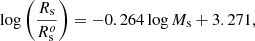
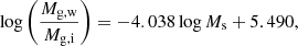
where Rs is the current effective radius of the galaxy,  the radius it would have if strictly following Eq. (3), and Mg, w/Mg, i the gas mass lost in the galactic wind normalized to the initial gas mass. The last relation shows that
  increases with Mg, w/Mg, i. The stronger the galactic wind, the larger the final effective radius. In other words, galaxies tend to depart from the locus represented by Eq. (3) and/or Eq. (26). In addition to this, we noted that the relative efficiency of galactic winds tends to decrease with increasing initial density of the proto-galaxy (compare models A and B in Table B.1). This means that the effect of galactic winds in inflating low-mass galaxies of high initial density is lower, meaning that their final radius will be closer to the value predicted by Eqs. (3) and/or (26). Our conclusion is that the flatter slope of the theoretical MRR in the monolithic scheme is likely caused by galactic winds.
(b) In the case of the hierarchical scenario, the situation is more complicated because mergers and galactic winds both act to inflate a galaxy. To clarify the issue, Chiosi & Carraro (2002) discussed the case of a merger between two galaxies calculated by Buonomo (2000) of which they knew every detail: a 2 × 10¹¹ M⊙ galaxy was simulated by merging two disc-like sub-units, each one with total mass (BM+DM) equal to 1 × 10¹¹ M⊙, and ratio of BM to DM equal to 0.1. At the time of encounter the mass in the stars of each subunit was about Ms = 6 × 10⁸ M⊙ and the mass in gas was Mg = 9.3 × 10⁹ M⊙. The merger was accompanied by little star formation, meaning that the total mass in stars, gas, and BM of the newly formed galaxy was Ms = 1.2 × 10⁹ M⊙, Mg = 1.8 × 10¹⁰ M⊙, and 2 × 10¹⁰ M⊙, respectively. The effective radius of the composite object was Rs = 8.4 kpc and its shape was similar to that of an elliptical one. The merger galaxy is shown in Fig. 6 by the big empty star; it resembles our Mod-B of comparable total star mass except for the fact that it is more diffuse. Based on these calculations, we estimate that merging two single disc-like objects made of stars and gas to build up a galaxy with twice as much total mass as the component galaxies would generate an elliptical-like galaxy, the star mass and effective radius of which are lower and higher, respectively, by ΔMs/Ms ≃ −0.9 and ΔRs/Rs ≃ 0.5 compared to the case of an elliptical of the same mass but obtained with the monolithic scheme. However, if mergers inflate the final object (see Hernquist 1992, 1993) and therefore explain the position of DGs (see also the many models of the Illustris database calculated in the hierarchical framework), they cannot explain the observational MRR of ETGs. In other words, mergers may act to build up a galaxy, but do not determine the final MRR.
5.3. Genesis of the true MRR
Considering these premises, we suggest that the observational MRR of ETGs, either that of Eqs. (2), (3), or (4), represents the locus on the MR plane of galaxies whose present-day structure closely mimics the ideal situation of mechanical (virial) equilibrium and passive evolution. Their MRR is also the boundary between permitted and forbidden regions of the MR plane. The DGs or less massive objects require a different interpretation, because they significantly depart from the above evolutionary scheme and the MRR that holds for ETGs.
To prove the above statement in a simple fashion we strictly follow the method proposed long ago by Chiosi & Carraro (2002), but updated taking into account the recent theoretical and observational data. To this aim, we draw in Fig. 10 two loci and a mass interval as a function of the initial density (redshift):
(a) The first locus is the present-day MRR traced by model galaxies of different mass but similar initial density with varying formation redshift. Most of this issue is examined in detail but from a different perspective in Sect. 3.4. The novelty here is to provide an easy-to-use relationship yielding the expected MRR of theoretical models as a function of the formation redshift zf for the bulk of the stellar content of a galaxy. Using all the models at our disposal, that is, those of Chiosi & Carraro (2002) and Merlin & Chiosi (2006, 2007), Merlin et al. (2010, 2012), Chiosi et al. (2012) we get the relation
![$$ \begin{aligned}&\log R_{\rm s} = [-1.172 - 0.412\, (1+z_{\rm f})] \nonumber \\&\qquad \quad + [0.244 + 0.0145 \, (1+z_{\rm f})] \, \log M_{\rm s} .\end{aligned} $$](/articles/aa/full_html/2020/11/aa38773-20/aa38773-20-eq44.gif)
The following cases are shown in Fig. 10: zf ≃ 1, zf ≃ 2, z ≃ 5, and zf ≃ 10. The procedure is easy thanks to the regular behavior of the models and the density–mass relationship of Eq. (26). This relationship is compatible with the MRRs predicted by Fan et al. (2010); see Eq. (12). Finally, it also agrees with the theoretical models of Illustris by Vogelsberger et al. (2014a,b).
(b) The second locus is the MRR for galaxies with the statistical maximum mass allowed by the underlying HGM at any redshift. This relationship can be derived (either graphically or numerically) from any HGM in the literature, such as for example those of Lukić et al. (2007), Angulo et al. (2012), or Behroozi et al. (2013). In Sect. 4.2 we derive this relation for the HGF of Lukić et al. (2007): see the analytical expression of Eq. (16) or its extension to the whole MR plane given by Eq. (17). However, for the sake of a very simple yet instructive analytical approach we prefer to make use here of the classical Press & Schechter (1974) function of halos as a sort of mass distribution function for galaxies: in the simplistic assumption of one galaxy per halo, it provides the relative number of galaxies per mass bin at varying redshift. Furthermore, we consider the cut-off mass  of the Press & Schechter (1974) function as the maximum mass limit of the galaxy masses at the current value of the redshift. According to the Press & Schechter (1974) formalism, this cut-off varies with the redshift according to
The exponent n is the slope of the initial power spectrum of the perturbations and MN is a suitable normalisation mass scale. At any redshift, most of the galaxies have total masses smaller than  , although higher values cannot be excluded. Indeed, the fractional mass in (or fractional number of) galaxies with mass greater than
  is a function of n. For n = −1.8, the percentage of galaxies in the mass interval
  amounts to about 15% and in the range
  to about 1%. Therefore, at any redshift galaxy masses up to say
  may occur with a sizable probability.
With the aid of the relationships presented in Tables B.1–B.3 (providing the mass in stars and effective radius of BM as a function of MT) and limited to the case with  for γ = 50 and power spectrum n = −1.8, we get

where Rs and Ms are in kiloparsecs and M⊙. These loci are shown in Fig. 10 by the dotted lines labelled with the redshift, namely z ≃ 1, ≃2, ≃5, and ≃10. On the MR plane, these loci represent the rightmost extension of the lines of constant density and hence the maximum galaxy mass. With decreasing redshift, the boundary progressively moves toward higher masses. Similar lines and conclusions can be recovered using the HGFs of Lukić et al. (2007), Angulo et al. (2012), or Behroozi et al. (2013).
(c) Finally, the third locus is the expected interval for Ms (the present-day star mass in a galaxy) for objects with total mass comprised between  and
and  as a function of the redshift. To this aim, the relation Ms(MT) has been plugged into relation (35) for
  . The permitted intervals are shown in Fig. 10 by the horizontal lines labelled
  . The interval for Ms going from 1010 M⊙ to 1012 M⊙ is fully compatible with a redshift interval for the formation of the majority of stars in a galaxy from 2 to 1. This interval is also the mass range over which at each redshift the probability of the occurrence of massive galaxies falls to negligible values. In other words, on the MR plane the right-hand border of the MRR has a natural width.
Having set the whole scene, we proceed to the final step. If our reasoning is correct, the basic relationship for ETGs, that of either Eqs. (3) or (26) but extended to the whole mass range of the objects under consideration (from GCs to GCGs), should correspond to the intersection of lines of constant initial density and the lines  for equal values of redshift, at least for all values of redshift greater than about 1. This indeed is what we see in Fig. 10 (the large empty squares). This result provides an analytical demonstration that the observational MRR stems from the product of two main factors: the mechanism governing galaxy formation and evolution (monolithic, early-hierarchical, or fully hierarchical) and the HGF and its variations with redshift. It follows from this analysis that the MRR is the locus where we find objects in mechanical (virial) equilibrium and at a passive or almost passive evolutionary stage. This MRR is mainly traced by ETGs, GCs, a few DGs, and GCGs; the large majority of DGs lie above it. Above, we put forward the physical reasons why DGs (with a few exceptions) cannot yet lie on this MRR, that is, because of the ongoing active star formation and strong galactic winds. This finding confirms the result obtained by D’Onofrio et al. (2019): only passive galaxies (strongly decreasing in luminosity as the redshift goes to zero) trace the MRR on the MR plane with a slope 0.5–1, the highest value being reached by objects that suffered the strongest luminosity decrease with redshift, that is, those that long ago ceased their stellar activity, likely the massive ones. Spiral galaxies occupy nearly the same location on the MR plane, suggesting that their ongoing star formation is not affecting the overall situation of mechanical equilibrium of the whole system.
Given that linear relations have been used (in compliance with the euclidean “ruler and compass” method), the result is a straight line illustrated by the large empty squares. The correct evaluation would be given by numerically folding the adopted HGF, Lukić et al. (2007) in our case, with the loci on the MR plane populated at the present time by galaxies of different mass but the same initial density born at different redshifts. The result is the crossed dark-red line shown in Fig. 10 represented by Eqs. (16) and/or (17).
Finally, it is worth noting that the slope of the MRR derived from the HGF is about 1 in the range of massive galaxies (say above 1012 M⊙), which is formally identical to the MRR that would be derived from the virial theorem. This coincidence might suggest that the observed MRR and its slope are driven by the virial condition, whereas the true driver of the MRR slope is the HGF, or rather, more precisely, its fall off toward high halo masses at any value of the redshift. On the other hand, all objects along the MRR are indeed in virial conditions once any mechanical process and star formation are at rest.
5.4. Possible effects blurring the MRR
Above, we showed that a tight MRR may result from first physical principles coupled to elementary cosmology. For the sake of completeness, we may turn the argument around and check whether or not, starting from an intrinsically sparse distribution of galaxies on the MR plane, one may recover a tight MRR as the result of some physical effects.
There are at least two important phenomena at work, namely mergers of two galaxies of different mass (and size) into a single object and matter ejection by a single galaxy by sudden injection of energy (e.g. AGN activity and/or galactic winds), that could change the position of a given galaxy on the MR plane and therefore scatter the expected distribution. Whether or not, on the contrary, starting from a scattered distribution of galaxies, they can give rise to more or less ordered sequence – such as that indicated by the MRR – is hard to prove, and unlikely to occur in the real world.
Minor and major mergers. In the hierarchical scenario, minor (unequal masses) and major (equal masses) mergers of low-mass galaxies into ones of larger masses is the paradigm mechanism by which galaxies acquire the dimensions and masses that we observe. There are many papers and even text books trying to resolve this issue, such as for example Binney & Tremaine (2008), Hopkins et al. (2008), Naab et al. (2009) to mention a few. The formalism in use here was suggested by Bernardi (2011, talk delivered at the University of Padova, priv. comm.). The process can be accompanied by star formation (so-called wet merger) which would spread the age and the metallicity of the stellar populations hosted by galaxies. This may cause some difficulties with the ETGs whose stars seem to be old with a rather narrow age range; we return to this below. Alternatively, the mergers can occur free of star formation (in this case they are referred to as dry mergers). Wet or dry, by how much a merger between two bodies of masses M1 and M2 and radii R1 and R2 can increase the mass and size of the daughter galaxy is unclear. For a pair of interacting virialised galaxies made of DM, we may assume that the total energy is given by the sum of kinetic and gravitational potential:

where Evir is the total virial energy of the two galaxies and Eint is the energy of interaction. This can be neglected with respect to the first one so that the total energies before merging are
where the σ are the velocity dispersions. After merging, the total energy of the system is
In a dissipationless process, during the merger the total energy is conserved, meaning that Ef = Ei. In the case of a major merger represented by M1 = M2 = Mi and Mf = 2Mi, we get
which means that the mass and radius are doubled, whereas σ remains unchanged. In the MR plane the displacement vector has slope Δlog R/Δlog M = 1 (van Dokkum et al. 2010).
In the case of a minor merger represented by Mf = (1 + f)Mi, where f is smaller than 1, the virial theorem (2K = −W with obvious meaning of the symbols) yields  , from which we get

When f << 1 we obtain

which means that the change in size is larger than the change in mass and also σ decreases. The displacement vector has slope Δlog R/Δlog M > 1 and likely close to 2 (van Dokkum et al. 2010).
Finally, we believe it noteworthy that the above formalism has been developed looking at the sole DM component of the interacting galaxies. How the BM component will behave during the merger event is not completely understood, and insufficient simulations are available to make solid predictions. Long tails of DM and BM are likely to develop, thus likely removing significant amounts of mass from the two components. The effect could be particularly relevant for BM because of the many implications for subsequent star formation (if any). In any case, mergers alone cannot be responsible for the well-behaved MRR, but would simply add some dispersion on it.
Puffing up and galactic winds. Rapid stripping or ejection of BM from galaxies may inflate them to larger dimensions. The idea goes back to Biermann & Shapiro (1979), who linked the formation of S0 galaxies to that of disc galaxies. Recently, these processes were reconsidered by Ragone-Figueroa & Granato (2011) to explain the observational evidence that most massive ETGs at redshift z ≥ 1 exhibit sizes smaller by a factor of a few than local galaxies of the same type and mass. These latter authors investigate the effect of BM loss triggered either by QSO and/or starburst-driven galactic winds or quiet gas restitution and ejection by stars at the end of their evolution, both concurring in a galaxy to eject a sizable fraction of the BM mass.
The evolution of the galaxy depends on the ejection timescale compared to the dynamical timescale. If the former is short compared to the latter (fast ejection) the ratio of the final to the initial radius is
and if Mf/Mi ≤ 0.5 the system becomes unbound and dissolves. If the ejection timescale is long then the conservation of adiabatic invariants yields
Thus, if the ejection is fast the size increase is more efficient, and if the ejection is slow the system remains bound independently of Mf/Mi. In this scheme the compact objects should transform into less massive and larger systems. This process could occur in two steps: a very fast at the beginning of the star forming history, and a slow one during the remaining life of the system. Indeed our NB-TSPH models only partly follow this scheme. The models have intense episodes of star formation and significant galactic winds but, on average, the general trend is toward larger star masses and almost constant radii. Whether or not this mechanism can account for the general distribution of galaxies on the MR plane is unclear6.
Geometrical effects. Guo et al. (2009) and van Dokkum et al. (2010) investigated the possibility that the MRR, at least for the most massive galaxies, is driven by a systematic variation of the Sersic index ns, parameterising the surface density profiles with the redshift. According to van Dokkum et al. (2010), in the context of the inside-out growth of a galaxy by accumulation of material, the variation of the effective radius Re (50% of the light) and Rs in turn, the Sersic index, and the galaxy mass is
which is accurate to 0.01 dex for 1 ≤ n ≤ 6. This means that the radius increases approximately linearly with the mass if the projected density follows an exponential law, but it goes as M1.8 for the de Vaucouleurs profile with ns = 4. This implies that strong evolution in the measured Re is expected in all inside-out growth scenarios irrespective of the physical mechanism, unless the density profiles are close to exponential. In our models, the Sersic index varies from ns ≃ 2 for the HDMM case to ns = 4 for the HDHM one. Therefore, the expected variation of the slope dlog Re/dlog M due to geometrical effects goes from about 1 to about 1.8. This implies that the displacement vector changes slope according to the Sersic index of the underlying galaxy. The slope increases from Re ∝ M to Re ∝ M2. Indeed, looking at the mean locus of galaxies in the MR plane, the slope increases moving toward the top right corner of the plane; in other words the band tends to bend toward higher radii as the mass increases, passing from 0.5 for the low-mass galaxies, to 1 for the intermediate-mass ones, to about 2 for those at the top end. van Dokkum et al. (2010) made use of the above relation to explain the steep slope of the MRR for galaxies measured at different redshifts (from z = 2 to z = 0) whose radii and masses seem to increase according to Re ∝ M2: 0.45 ≤ log Re ≤ 1.1 and 11.15 ≤ M(M⊙) ≤ 11.45. At high redshift (z ≃ 2), these galaxies have smaller effective radii and profiles that are closer to exponential, whereas at low redshift (z ≃ 0) the radii become larger and the profiles approach the de Vaucouleurs law. It seems that the size and hence the density is correlated with the Sersic profile which in turn drives the displacement vector in the MR plane. However, it is worth recalling that exactly the same trend of the MRR is also shown by the CGS in the mass range of interest, thus partially weakening the argument based on geometrical effects. It is likely that both act simultaneously to shape the top end of the MRR.
5.5. Compact objects at high redshift: a few remarks
In recent years, convincing evidence has been gathered suggesting that, at relatively high redshifts, there are objects of comparable mass to that of nearby massive galaxies but with smaller dimensions. These “compact galaxies” are found up to z ≥ 3 with stellar masses from 1010 to 1012 M⊙ and half-light radii from 0.4 to 5 kpc (i.e. three to four times more compact than local counterparts of the same mass), and in nearly similar proportions there are galaxies with the same mass but a variety of dimensions (e.g. Mancini et al. 2009; Valentinuzzi et al. 2010) and bulge to disc ratios (e.g. Karim et al. 2011). Although the detection of compact galaxies at high redshift may be affected by observational biases (e.g. Mancini et al. 2009), extremely deep imaging (e.g. Szomoru et al. 2010), lensing (e.g. Auger et al. 2011; Newton et al. 2011), available measurements of very high-velocity dispersions (e.g. Cenarro & Trujillo 2009; Cappellari et al. 2009; van Dokkum et al. 2009; van de Sande et al. 2011), and measurements of surface brightness (Szomoru et al. 2012) are confirming their compactness. Furthermore, according to Saracco et al. (2011), compact galaxies tend to complete their star forming activity at z > 5, whereas larger galaxies of similar mass tend to have a younger stellar content, suggesting that the structure of a galaxy may be related to its star formation activity (see Mosleh et al. 2011; Shankar et al. 2013, and references therein).
The sample of compact galaxies we are going to consider is gathered from different sources and spans an ample range of redshifts. Data for low-mass objects are taken from Cimatti et al. (2004), Daddi et al. (2005), Maraston et al. (2006), Toft et al. (2007), Zirm et al. (2007), Cimatti et al. (2008), McGrath et al. (2008), van Dokkum et al. (2009), Gadotti (2009), and Fisher & Drory (2011); see also Shankar et al. (2013). The masses (in M⊙) and radii (in kiloparsecs) fall in the ranges 9 < log Ms < 11 and 0.3 < log Rs < 1.3, respectively. They define a mean relation represented by

It is worth emphasizing that this relation runs almost parallel to that drawn by the SDSS data for ETGs of Bernardi et al. (2010). In the high-mass range, we have data from Bezanson et al. (2009), Damjanov et al. (2009), Mancini et al. (2010), Longhetti et al. (2007), and recently Tiret et al. (2011). The estimated masses and radii (in the same units) span the intervals 11 < log Ms < 12 and 0.4 < log R1/2 < 1.3. They define a mean relation given by

Remarkably, the slope of the above relation is nearly twice that in the lower mass interval and intersects the region of the most massive and widest ETGs in the Bernardi et al. (2010) sample. For more details on the subject and the current explanation for both compact and extended objects at the same redshift (similar luminosity and hence mass) see Shankar et al. (2013). Even if a formal comparison between ETGs and compact galaxies is not possible because two samples of data are not fully homogeneous, an idea of their relative positions on the MR plane can be inferred.
Compact galaxies on the MR plane are shown Fig. 11 together with normal ETGs and theoretical models. More precisely, the blue filled circles are the compact galaxies, the red open circles the normal ETGs, the large filled circles the theoretical models of Table B.3, and finally the solid lines show the theoretical present-day MRRs of relation (34) for galaxies whose initial collapse took place at different redshifts zf = 1, 5, 8, and 10 (iso-initial-density lines).
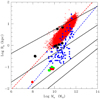 |
Fig. 11. log[Rs] vs. log[Ms] relation for compact galaxies (filled blue circles) and their best fit (blue dashed line). The red open circles are the ETGs from Bernardi et al. (2010) plotted here for comparison, and the red dashed line is their best-fit. The large filled circles are the 12 ancillary models (black the efficiency of star formation ϵsff = 1, green for ϵsff = 0.5, and red for ϵsff = 0.1). The thin straight lines are the present-day MRRs of model galaxies that started their collapse at different redshifts, namely zf = 1, zf = 5, zf = 8, and zf = 10 from top to bottom. The lines are given by Eq. (34). |
First of all, we note that a significant number of compact galaxies fall into the region of classical ETGs, and therefore in terms of their mass they appear similar to them. Issues arise from the fact that their high redshift indicates a remote epoch in which according to the classical view of galaxy assembly they should not occur. The remaining compact galaxies fall below the ETGs, meaning that for their mass the dimensions are significantly smaller. The comparison with the iso-density lines of galaxy models would imply a rather high redshift and high initial density in turn. The upper value for the formation redshift is zf ≃ 8.
Concerning compact galaxies, several questions arise (among others): How can these compact (and high-mass) objects exist at high redshift? How do they evolve? What are their counterparts in the local Universe? Does their position provide information on the initial density of the collapsing object, or perhaps something else?
Compact galaxies with estimated star mass in the range 1010 to 5 × 10¹² M⊙ – see for instance the data by Gadotti (2009), Bezanson et al. (2009), Damjanov et al. (2009), Mancini et al. (2010), Fisher & Drory (2011), and Tiret et al. (2011) – likely belong to systems made of DM + BM of significantly greater halo mass. An estimate of this latter can be obtained from the ratio MD = m Ms. We adopt here m = 10, which according to the data reported in Fig. A.1 corresponds to the mean value of the Ms/MD for galaxies in this mass range.
According to Lukić et al. (2007), the probability of occurrence per (Mpc h−1)3 for galaxies with total mass in the range (1010 − 1011)M⊙ goes from a few 10−1 at z ≃ 1 to below 10−5 at z ≃ 16, whereas for objects in the mass range (1012 − 1013)M⊙ the probability falls from a few 10−3 at z ≃ 1 to below 10−5 at redshift z ≃ 11. These probabilities albeit small are still significant for a total observed volume of about 108 Mpc3. Similar considerations can be made for the objects in the lower range of mass even though there is a greater probability of them coming into existence at high redshifts. Therefore, massive galaxies with very high initial density (high formation redshift) are possible.
Looking at the position of our ancillary models (see Table B.3 for the data) on the MR plane of Fig. 11, two possible explanations can be put forward: (i) very high redshift (say up to about 8) and hence very high mean density environment; (ii) high redshift (say about 5) and hence lower mean density environment (in both cases we assume that the initial over-density of the collapsing halo is the same) but intrinsically less efficient star formation. The ancillary models show that in both case, compact objects are possible. The case of high redshifts and high initial densities is not particularly interesting; this case could correspond to an epoch in which globular clusters and/or bulges of galaxies are generated. On the contrary, in the current view of galaxy formation by mergers taking place all over the Hubble time and initiated at about zf = 5 (in any case galaxy assembly is completed in the redshift interval z = 2−5), the role played by the star-formation threshold density has never been fully highlighted and therefore deserves some attention. If for any reason star formation is inhibited at the gas densities that were typical of normal ETGs, the primordial gas can collapse in the potential well of DM + BM to higher densities and smaller radii in turn. From this time, the dimensions of the star forming regions can either remain nearly constant or increase as more stars are gradually formed by the inflowing gas. In this context, the MRR of compact galaxies should mimic that of normal galaxies. We argue above that this latter mirrors the shape of the cosmic galaxy shepherd on the MR plane. Indeed the sequence of compact galaxies changes its slope from 0.5 to 1 and even higher as the mass goes toward the upper limit. Mergers and mass ejection episodes may occur, thus inflating the system as already reported above and therefore blur the ideal sequence. This explanation in terms of the threshold density for star formation does not contradict the suggestion that these objects could be the bulges of bigger galaxies (Graham et al. 2011).
Finally, there is another parameter to consider, namely the velocity dispersion fσ. According to Eq. (12), at given total mass, redshift and all remaining parameters, the radius Rs scales with (1.5/fσ)2. It is likely that a compact object has a higher velocity dispersion compared to that of a normal object. Passing from the reference value fσ = 1 to fσ = 2, the radius goes down by a factor of 0.5. Therefore, given the position of a compact object on the MR plane, the associated initial redshift would turn out to be about a factor of two smaller than before, thus alleviating the initial redshift required to explain the position of compact galaxies on the MR plane. We believe the whole subject merits deeper investigation.
6. General remarks and conclusions
What can we learn from all these observational hints and the striking coincidence between data and theory? In search of a coherent picture, we suggest the following scenario:
(i) According to their initial density, galaxies of a given total mass will be distributed over the MR plane along lines of type A and/or B and/or C. The initial density is not constant but decreases as zf tends to zero. The permitted mass interval for the total (and baryonic) mass of the galaxies is not constant, but increases at decreasing redshift. At redshifts of about 1 to 2, galaxies with total mass up to a few 1012 M⊙ are in place and their MRR will extend up to the range populated by the galaxies we see today.
(ii) The expectation is that galaxies of any mass and initial density crowd a strip bounded by the lines of maximum and minimum initial density (say redshifts from about 10 to 1–2) and the line corresponding to their maximum mass in the HGF for the same redshifts.
(iii) In this context, the semi-plane below either relation (26) in the simple description or relation (17) based on the cosmic galaxy shepherd, and the HGF in turn, is void of galaxies, because they would be too massive at a given initial density (redshift) to be compatible with the maximum mass of the HGF in general for all values of the redshift.
(iv) In the semi-plane above relation (26) and/or (17), the available data are not of sufficient quantity to allow for robust statistical analysis, meaning that in the range of low-mass galaxies we have only those of the Local Group (M32 and ωCen included). Dwarf galaxies of large effective radius are simply not in the sample. Observations of the Fornax cluster (Im et al. 2001) revealed a new type of DG with intrinsic sizes of about 100 pc. These are more compact and less luminous than other known compact DGs, yet are much brighter than globular clusters. Their absolute magnitude is about MB = −13 (two magnitudes fainter than M32). Do these objects represent the low-mass tail of galaxies falling along line A in Fig. 10? More observational data may help to clarify this issue.
(vi) GCs are more difficult to discuss because those we have considered are bound to the Milky Way, meaning that they have certainly suffered many external (and internal) dynamical processes that may have changed their present mass and radius.
(vii) Finally, we come to GCGs. The masses of their bulk stellar content and the half-mass radii of the ideal sphere in which stars are contained, are still highly uncertain, meaning that on the MR plane they do not trace a sharp MRR but rather a broad region. Part of the scatter is perhaps due to GCGs still evolving towards the equilibrium state, and another part to observational uncertainties. Suffice it to note here that the same theoretical MRR can pass through all the regions of the MR plane crowded by objects going from GCs to GCGs.
(viii) In conclusion, we endeavor to speculate on the origin of the present-day MRRs and their differences passing from GCs to DGs, ETGs, and GCGs. The focus has been on DGs and ETGs, however GCs and GCGs are also considered. For all of them, we suggest a common origin stemming from the interplay between several processes, such as for example the initial density together with total mass, which drive the SFH; the efficiency of energy feedback in triggering galactic winds that affect the mass and the size of the objects; and the merger history of a galaxy and the steady increase of the maximum mass reachable by the HGF at decreasing redshift and/or decreasing mean density of the Universe. High-density (low-mass) objects are the first to form stars in the remote past followed by objects of lower density (higher mass). The MRRs of Eqs. (3) or (26) simply reflect the above interplay. Galaxies as massive as a typical 1012 M⊙ object can be in place at redshifts from 2 to 1. After the first initial activity, passive evolution is expected. This generates the MRR of dynamically stable and passively evolving objects in virial conditions, the shape of which is driven by the cosmological distribution (mass and relative number density) of the halos hosting the visible galaxy. Since the HGF is not a linear function, the slope of the MRR continuously varies from ≃0.5 to ≃1. Objects in similar physical conditions (passive evolution and virial regime) but with lower mass (say up to 1010 M⊙) closely follow the MRR of the dissipationless case (slope of about 0.5 or so) and yet are in virial conditions (see GCs and DGs like ωCen and M32). All other galaxies, being far from these ideal conditions because of active star formation, the presence of galactic winds, the occurrence of repeated mergers, and so on, strongly depart from the ideal MRR of objects in mechanical and thermal equilibrium. Information for GCGs is still in being gathered, and so no firm conclusions can yet be drawn, even though they seem to fit this scenario.
The selection conditions are fracDeV = 1 and b/a > 0.6, and therefore the sample is dominated by elliptical galaxies (see Bernardi et al. (2010) for more details).
This has been derived from an analytical interpolation of the data presented in Fig. 1 of Lukić et al. (2007).
The discussion by Chiosi & Carraro (2002) on this issue is still valid, and is strengthened by the new NB-TSPH models used in this study. In their analysis, Chiosi & Carraro (2002) showed that the discrepancy between the slopes of the MRR traced by models and data for ETGs cannot be ascribed to mergers, because in this case the models would fall even farther out with respect to existing observational data.
Acknowledgments
We like to thanks Prof. L. Secco and Dr. R. Caimmi for very useful discussions on many aspects of this study. C.C. thanks the Department of Physics and Astronomy of the Padua University for the hospitality and computational support.
References
- Agertz, O., & Kravtsov, A. V. 2016, ApJ, 824, 79 [CrossRef] [Google Scholar]
- Angulo, R. E., Springel, V., White, S. D. M., et al. 2012, MNRAS, 426, 2046 [CrossRef] [Google Scholar]
- Auger, M. W., Treu, T., Brewer, B. J., & Marshall, P. J. 2011, MNRAS, 411, L6 [CrossRef] [Google Scholar]
- Behroozi, P. S., Wechsler, R. H., Wu, H.-Y., et al. 2013, ApJ, 763, 18 [NASA ADS] [CrossRef] [Google Scholar]
- Bernardi, M., Shankar, F., Hyde, J. B., et al. 2010, MNRAS, 404, 2087 [NASA ADS] [Google Scholar]
- Bernardi, M., Roche, N., Shankar, F., & Sheth, R. K. 2011, MNRAS, 412, L6 [NASA ADS] [CrossRef] [Google Scholar]
- Bernardi, M., Meert, A., Vikram, V., et al. 2014, MNRAS, 443, 874 [NASA ADS] [CrossRef] [Google Scholar]
- Bezanson, R., van Dokkum, P. G., Tal, T., et al. 2009, ApJ, 697, 1290 [NASA ADS] [CrossRef] [Google Scholar]
- Biermann, P., & Shapiro, S. L. 1979, ApJ, 230, L33 [NASA ADS] [CrossRef] [Google Scholar]
- Binney, J., & Tremaine, S. 2008, Galactic Dynamics: Second Edition (Princeton University Press) [Google Scholar]
- Blumenthal, G. R., Faber, S. M., Primack, J. R., & Rees, M. J. 1984, Nature, 311, 517 [NASA ADS] [CrossRef] [Google Scholar]
- Bryan, G. L., & Norman, M. L. 1998, ApJ, 495, 80 [NASA ADS] [CrossRef] [Google Scholar]
- Buonomo, F. 2000, PhD Thesis, Astronomy Department, Padova University, Italy [Google Scholar]
- Burstein, D., Bender, R., Faber, S., & Nolthenius, R. 1997, AJ, 114, 1365 [NASA ADS] [CrossRef] [Google Scholar]
- Caminha, G. B., Grillo, C., Rosati, P., et al. 2017, A&A, 607, A93 [NASA ADS] [CrossRef] [EDP Sciences] [Google Scholar]
- Cappellari, M., di Serego Alighieri, S., Cimatti, A., et al. 2009, ApJ, 704, L34 [NASA ADS] [CrossRef] [Google Scholar]
- Cariddi, S., D’Onofrio, M., Fasano, G., et al. 2018, A&A, 609, A133 [NASA ADS] [CrossRef] [EDP Sciences] [Google Scholar]
- Cava, A., Bettoni, D., Poggianti, B. M., et al. 2009, A&A, 495, 707 [NASA ADS] [CrossRef] [EDP Sciences] [Google Scholar]
- Cenarro, A. J., & Trujillo, I. 2009, ApJ, 696, L43 [NASA ADS] [CrossRef] [Google Scholar]
- Chiosi, C., & Carraro, G. 2002, MNRAS, 335, 335 [NASA ADS] [CrossRef] [Google Scholar]
- Chiosi, C., Merlin, E., & Piovan, L. 2012, ArXiv e-prints [arXiv:1206.2532] [Google Scholar]
- Cimatti, A., Daddi, E., Renzini, A., et al. 2004, Nature, 430, 184 [NASA ADS] [CrossRef] [PubMed] [Google Scholar]
- Cimatti, A., Cassata, P., Pozzetti, L., et al. 2008, A&A, 482, 21 [NASA ADS] [CrossRef] [EDP Sciences] [Google Scholar]
- Corwin, H. G., Jr, Buta, R. J., & de Vaucouleurs, G. 1994, AJ, 108, 2128 [NASA ADS] [CrossRef] [Google Scholar]
- Daddi, E., Renzini, A., Pirzkal, N., et al. 2005, ApJ, 626, 680 [NASA ADS] [CrossRef] [Google Scholar]
- Damjanov, I., McCarthy, P. J., Abraham, R. G., et al. 2009, ApJ, 695, 101 [NASA ADS] [CrossRef] [Google Scholar]
- de Vaucouleurs, G., de Vaucouleurs, A., Corwin, Jr., H. G., et al. 1991, Third Reference Catalogue of Bright Galaxies (New York, NY, USA: Springer) [Google Scholar]
- D’Onofrio, M., Bindoni, D., Fasano, G., et al. 2014, A&A, 572, A87 [NASA ADS] [CrossRef] [EDP Sciences] [Google Scholar]
- D’Onofrio, M., Sciarratta, M., Cariddi, S., Marziani, P., & Chiosi, C. 2019, ApJ, 875, 103 [CrossRef] [Google Scholar]
- D’Onofrio, M., Chiosi, C., Sciarratta, M., & Marziani, P. 2020, A&A, 641, A94 [CrossRef] [EDP Sciences] [Google Scholar]
- Engler, C., Pillepich, A., Joshi, G. D., et al. 2020, MNRAS, submitted [arXiv:2002.11119] [Google Scholar]
- Faber, S. M. 1984, in Galaxy Formation and Cosmology, in Large-Scale Structure of the Universe, Cosmology and Fundamental Physics, Proceedings of the 1st ESO/CERN Symposium held 21-25 November, 1983 at CERN, Geneva, eds. G. Setti, & L. Van Hove, 187 [Google Scholar]
- Fan, L., Lapi, A., Bressan, A., et al. 2010, ApJ, 718, 1460 [NASA ADS] [CrossRef] [Google Scholar]
- Fasano, G., Marmo, C., Varela, J., et al. 2006, A&A, 445, 805 [NASA ADS] [CrossRef] [EDP Sciences] [Google Scholar]
- Fasano, G., Vanzella, E., Dressler, A., et al. 2012, MNRAS, 420, 926 [Google Scholar]
- Fisher, D. B., & Drory, N. 2011, ApJ, 733, L47 [NASA ADS] [CrossRef] [Google Scholar]
- Fritz, J., Poggianti, B. M., Bettoni, D., et al. 2007, A&A, 470, 137 [NASA ADS] [CrossRef] [EDP Sciences] [Google Scholar]
- Fritz, J., Poggianti, B. M., Cava, A., et al. 2011, A&A, 526, A45 [NASA ADS] [CrossRef] [EDP Sciences] [Google Scholar]
- Gadotti, D. A. 2009, MNRAS, 393, 1531 [NASA ADS] [CrossRef] [Google Scholar]
- Geha, M., Blanton, M. R., Masjedi, M., & West, A. A. 2006, ApJ, 653, 240 [NASA ADS] [CrossRef] [Google Scholar]
- Genel, S., Vogelsberger, M., Springel, V., et al. 2014, MNRAS, 445, 175 [Google Scholar]
- Genel, S., Nelson, D., Pillepich, A., et al. 2018, MNRAS, 474, 3976 [NASA ADS] [CrossRef] [Google Scholar]
- Girelli, G., Pozzetti, L., Bolzonella, M., et al. 2020, A&A, 634, A135 [CrossRef] [EDP Sciences] [Google Scholar]
- Gott, J. R., III, & Rees, M. J. 1975, A&A, 45, 365 [Google Scholar]
- Graham, A. W. 2011, in EAS Pub. Ser., eds. M. Koleva, P. Prugniel, & I. Vauglin, 48, 231 [CrossRef] [Google Scholar]
- Graham, A. W. 2013, in Elliptical and Disk Galaxy Structure and Modern Scaling Laws, in Planets, Stars and Stellar Systems, eds. T. D. Oswalt, & W. C. Keel (Dordrecht: Springer Science+Business Media) 6, 91 [Google Scholar]
- Gullieuszik, M., Poggianti, B., Fasano, G., et al. 2015, A&A, 581, A41 [NASA ADS] [CrossRef] [EDP Sciences] [Google Scholar]
- Guo, Y., McIntosh, D. H., Mo, H. J., et al. 2009, MNRAS, 398, 1129 [NASA ADS] [CrossRef] [Google Scholar]
- Hamraz, E., Peletier, R. F., Khosroshahi, H. G., et al. 2019, VizieR Online Data Catalog: J/A+A/625/A94 [Google Scholar]
- Hernquist, L. 1992, ApJ, 400, 460 [NASA ADS] [CrossRef] [Google Scholar]
- Hernquist, L. 1993, ApJ, 409, 548 [NASA ADS] [CrossRef] [Google Scholar]
- Hinshaw, G., Larson, D., Komatsu, E., et al. 2013, ApJS, 208, 19 [NASA ADS] [CrossRef] [Google Scholar]
- Hopkins, P. F., Hernquist, L., Cox, T. J., & Kereš, D. 2008, ApJS, 175, 356 [NASA ADS] [CrossRef] [Google Scholar]
- Huang, K.-H., Fall, S. M., Ferguson, H. C., et al. 2017, ApJ, 838, 6 [NASA ADS] [CrossRef] [Google Scholar]
- Im, M., Faber, S. M., Gebhardt, K., et al. 2001, AJ, 122, 750 [NASA ADS] [CrossRef] [Google Scholar]
- Karim, A., Schinnerer, E., Martínez-Sansigre, A., et al. 2011, ApJ, 730, 61 [NASA ADS] [CrossRef] [Google Scholar]
- Kissler-Patig, M., Jordán, A., & Bastian, N. 2006, A&A, 448, 1031 [NASA ADS] [CrossRef] [EDP Sciences] [Google Scholar]
- Krumholz, M. R., & Tan, J. C. 2007, ApJ, 654, 304 [NASA ADS] [CrossRef] [Google Scholar]
- Kuchner, U., Ziegler, B., Verdugo, M., Bamford, S., & Häußler, B. 2017, A&A, 604, A54 [NASA ADS] [CrossRef] [EDP Sciences] [Google Scholar]
- Lada, C. J., & Lada, E. A. 2003, ARA&A, 41, 57 [NASA ADS] [CrossRef] [Google Scholar]
- Longhetti, M., Saracco, P., Severgnini, P., et al. 2007, MNRAS, 374, 614 [NASA ADS] [CrossRef] [Google Scholar]
- Lukić, Z., Heitmann, K., Habib, S., Bashinsky, S., & Ricker, P. M. 2007, ApJ, 671, 1160 [NASA ADS] [CrossRef] [Google Scholar]
- Mancini, C., Matute, I., Cimatti, A., et al. 2009, A&A, 500, 705 [NASA ADS] [CrossRef] [EDP Sciences] [Google Scholar]
- Mancini, C., Daddi, E., Renzini, A., et al. 2010, MNRAS, 401, 933 [NASA ADS] [CrossRef] [Google Scholar]
- Maraston, C., Daddi, E., Renzini, A., et al. 2006, ApJ, 652, 85 [NASA ADS] [CrossRef] [Google Scholar]
- McGrath, E. J., Stockton, A., Canalizo, G., Iye, M., & Maihara, T. 2008, ApJ, 682, 303 [NASA ADS] [CrossRef] [Google Scholar]
- Merlin, E., & Chiosi, C. 2006, A&A, 457, 437 [NASA ADS] [CrossRef] [EDP Sciences] [Google Scholar]
- Merlin, E., & Chiosi, C. 2007, A&A, 473, 733 [NASA ADS] [CrossRef] [EDP Sciences] [Google Scholar]
- Merlin, E., Buonomo, U., Grassi, T., Piovan, L., & Chiosi, C. 2010, A&A, 513, A36 [NASA ADS] [CrossRef] [EDP Sciences] [Google Scholar]
- Merlin, E., Chiosi, C., Piovan, L., et al. 2012, MNRAS, 427, 1530 [NASA ADS] [CrossRef] [Google Scholar]
- Moretti, A., Poggianti, B. M., Fasano, G., et al. 2014, A&A, 564, A138 [NASA ADS] [CrossRef] [EDP Sciences] [Google Scholar]
- Moretti, A., Gullieuszik, M., Poggianti, B., et al. 2017, A&A, 599, A81 [NASA ADS] [CrossRef] [EDP Sciences] [Google Scholar]
- Mosleh, M., Williams, R. J., Franx, M., & Kriek, M. 2011, ApJ, 727, 5 [NASA ADS] [CrossRef] [Google Scholar]
- Naab, T., Johansson, P. H., & Ostriker, J. P. 2009, ApJ, 699, L178 [NASA ADS] [CrossRef] [Google Scholar]
- Nelson, D., Pillepich, A., Genel, S., et al. 2015, Astron. Comput., 13, 12 [NASA ADS] [CrossRef] [Google Scholar]
- Newton, E. R., Marshall, P. J., Treu, T., et al. 2011, ApJ, 734, 104 [CrossRef] [Google Scholar]
- Pasquato, M., & Bertin, G. 2008, A&A, 489, 1079 [NASA ADS] [CrossRef] [EDP Sciences] [Google Scholar]
- Press, W. H., & Schechter, P. 1974, ApJ, 187, 425 [NASA ADS] [CrossRef] [Google Scholar]
- Ragone-Figueroa, C., & Granato, G. L. 2011, MNRAS, 414, 3690 [NASA ADS] [CrossRef] [Google Scholar]
- Sanchez Almeida, J. 2020, MNRAS, 495, 78 [Google Scholar]
- Saracco, P., Longhetti, M., & Gargiulo, A. 2011, MNRAS, 412, 2707 [NASA ADS] [CrossRef] [Google Scholar]
- Sciarratta, M., Chiosi, C., D’Onofrio, M., & Cariddi, S. 2019, ApJ, 870, 70 [NASA ADS] [CrossRef] [Google Scholar]
- Shankar, F., Lapi, A., Salucci, P., De Zotti, G., & Danese, L. 2006, ApJ, 643, 14 [NASA ADS] [CrossRef] [MathSciNet] [Google Scholar]
- Shankar, F., Marulli, F., Bernardi, M., et al. 2013, MNRAS, 428, 109 [NASA ADS] [CrossRef] [Google Scholar]
- Shen, S., Mo, H. J., White, S. D. M., et al. 2003, MNRAS, 343, 978 [NASA ADS] [CrossRef] [Google Scholar]
- Somerville, R. S., Behroozi, P., Pandya, V., et al. 2018, MNRAS, 473, 2714 [NASA ADS] [CrossRef] [Google Scholar]
- Springel, V., White, S. D. M., Jenkins, A., et al. 2005, Nature, 435, 629 [NASA ADS] [CrossRef] [PubMed] [Google Scholar]
- Szomoru, D., Franx, M., van Dokkum, P. G., et al. 2010, ApJ, 714, L244 [NASA ADS] [CrossRef] [Google Scholar]
- Szomoru, D., Franx, M., & van Dokkum, P. G. 2012, ApJ, 749, 121 [NASA ADS] [CrossRef] [Google Scholar]
- Terrazas, B. A., Bell, E. F., Pillepich, A., et al. 2020, MNRAS, 493, 1888 [Google Scholar]
- Tiret, O., Salucci, P., Bernardi, M., Maraston, C., & Pforr, J. 2011, MNRAS, 411, 1435 [NASA ADS] [CrossRef] [Google Scholar]
- Toft, S., van Dokkum, P., Franx, M., et al. 2007, ApJ, 671, 285 [NASA ADS] [CrossRef] [MathSciNet] [Google Scholar]
- Valentinuzzi, T., Fritz, J., Poggianti, B. M., et al. 2010, ApJ, 712, 226 [NASA ADS] [CrossRef] [Google Scholar]
- Valentinuzzi, T., Poggianti, B. M., Fasano, G., et al. 2011, A&A, 536, A34 [NASA ADS] [CrossRef] [EDP Sciences] [Google Scholar]
- van de Sande, J., Kriek, M., Franx, M., et al. 2011, ApJ, 736, L9+ [NASA ADS] [CrossRef] [Google Scholar]
- van Dokkum, P. G., Kriek, M., & Franx, M. 2009, Nature, 460, 717 [NASA ADS] [CrossRef] [PubMed] [Google Scholar]
- van Dokkum, P. G., Whitaker, K. E., Brammer, G., et al. 2010, ApJ, 709, 1018 [NASA ADS] [CrossRef] [Google Scholar]
- Varela, J., D’Onofrio, M., Marmo, C., et al. 2009, A&A, 497, 667 [NASA ADS] [CrossRef] [EDP Sciences] [Google Scholar]
- Vogelsberger, M., Genel, S., Springel, V., et al. 2014a, Nature, 509, 177 [NASA ADS] [CrossRef] [Google Scholar]
- Vogelsberger, M., Genel, S., Springel, V., et al. 2014b, MNRAS, 444, 1518 [NASA ADS] [CrossRef] [Google Scholar]
- Warren, S., Lawrence, A., Almaini, O., et al. 2006, Messenger, 126, 7 [Google Scholar]
- Woo, J., Courteau, S., & Dekel, A. 2008, MNRAS, 390, 1453 [NASA ADS] [Google Scholar]
- Zirm, A. W., van der Wel, A., Franx, M., et al. 2007, ApJ, 656, 66 [NASA ADS] [CrossRef] [Google Scholar]
Appendix A: The stellar-to-halo mass relation
The ratio Ms/MD (and its inverse MD/Ms) are key quantities in the calculation of the (half-mass or effective) radius of the stellar component of a galaxy; see Eq. (12) of Sect. 4. The analysis of the Illustris data and the inspection of Tables B.1–B.3 show that the ratios Ms/MD and MD/Ms in turn depend on the total mass of the galaxy and the redshift zf at which the bulk of star formation occurs.
The dependence of the ratio Ms/MD on MD and redshift z for the Illustris data is shown in Fig. A.1. For low values of the redshift (say below 0.6), this ratio gently decreases with the mass MD (low-mass galaxies are slightly more efficient in building their stellar content); the opposite occurs for higher redshifts, where the ratio Ms/MD increases with MD, i.e. the stellar mass built-up in low-mass galaxies is expected to be less than in the massive ones.
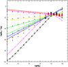 |
Fig. A.1. Relations Ms/MDMD at different redshifts for theoretical models (all masses are in solar units). The dotted lines of different colours correspond to the eight values of the redshift z = 0 and z = 0.2 (top, red), z = 0.6, z = 1.0 (intermediate, yellow), z = 1.6 and z = 2.2 (intermediate, green), z = 3 and to z = 4 (bottom, blue). The black dots are the values predicted by Eq. (A.1) at varying log MD from 4 to 14 in steps of 1 and redshift z from 0 to 4 in steps of 1, respectively. The large red and golden circles are the combination of Eqs. (A.3) and (A.2), respectively. The open magenta (z = 0) and black (z = 3.95) circles are relation Ms/MD vs. MD at different redshifts according to Girelli et al. (2020). We note how all relations agree with each other at log MD ≃ 12 whereas they badly disagree at lower values of MD. |
With the aid of the theoretical data for MD and Ms presented in Sect.4, we derive an analytical expression interpolating the ratio Ms/MD(MD, z) as a function of MD and z:
![$$ \begin{aligned} \log \frac{M_{\rm s}}{M_{\rm D}}= [0.218\,z - 0.101] \, \log M_{\rm D} + [0.169 \, z - 2.227 ] ,\end{aligned} $$](/articles/aa/full_html/2020/11/aa38773-20/aa38773-20-eq71.gif)
where the halo mass goes from 104 M⊙ to 1014 M⊙ and the redshift from 0 to 4. The ratios Ms/MD predicted by Eq. (A.1) are indicated by the small black dots of Fig. A.1. The range of application of relation (A.1) is 0 ≤ z ≤ 4.
Similar relationships for the ratio m = MD/Ms can be found in the literature; see e.g. Fan et al. (2010), Shankar et al. (2006), and more recently Girelli et al. (2020).
For MD ≥ 1011 M⊙, Fan et al. (2010) proposed the relation
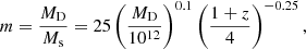
from which we derive the ratio Ms/MD shown in Fig. A.1 by the red circles. In practice, there is no dependence on the redshift.
Remarkably, the Fan et al. (2010) curve agrees with the one we derived from the Illustris models for values of the redshift smaller than about 1.6 (the slope is almost identical).
Shankar et al. (2006, and references there in) presented a detailed analysis of the dependence of Ms on MD. First, they suggested that for MD < 1011 M⊙ the relation should be
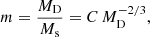
with C being a suitable proportionality constant to be determined. By imposing equality between the values of m determined with the two above relationships at the transition mass MD ≥ 1011 M⊙, the proportionality constant is log C = 9.044. The ratios MD/Ms predicted by Eq. (A.3) are shown in Fig. A.1 by the dark golden circles. It is worth noting that the Shankar et al. (2006) relation agrees with that of the Illustris models for redshifts in the range from 2 to 4.
Amazingly, it is worth noting that in Fig. A.1 the linear extrapolation of the Fan et al. (2010) relationship (red circles) to lower masses and the linear extrapolation of the Shankar et al. (2006) curve (dark golden circles) to higher values of the mass encompass the theoretical predictions from the Illustris models for all the values of the redshift.
Second, Shankar et al. (2006) derived an analytical expression for the relation between Ms and MD,
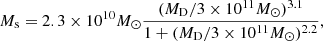
for MD ≥ 1011 M⊙. In this relation there is no explicit dependence on the redshift. The ratios Ms/MD predicted by Eq. (A.4) are shown in Fig. A.1 by the black filled squares. Equation (A.4) predicts ratios m(MD, z) that agree with those from Eq. (A.1) derived from Illustris data, Eq. (A.2) from Fan et al. (2010), and Eq. (A.3) only in the region around log(MD) ≃ 12 and z ≃ 0.
In a very recent study, Girelli et al. (2020) thoroughly investigated the stellar-to-halo mass ratio of galaxies (Ms/MD in the mass interval 1011 < MD < 1015 and redshifts from z = 0 to z = 4. These latter authors use a statistical approach to link the observed galaxy stellar mass function on the COSMOS field to the halo mass function from the ΛCDM-Dustgrain simulation and derive an empirical model to describe the variation of the stellar-to-halo mass ratio as a function of redshift. Finally, they provide analytical expressions for the function Ms(MD, z). The relations Ms/MD versus MD as a function of the redshift obtained with the formalism of Girelli et al. (2020) are also shown in Fig. A.1 (the magenta and dark-olive-green open circles joined by dashed lines of the same colour) and are compared with the results of the present study. For a similar analysis, see the study of Engler et al. (2020).
It is immediately evident that while all studies agree on the Ms/MD ratios for objects with halo mass in the interval 11.5 ≤ log MD ≤ 12.5 nearly independently of the redshift, they strongly disagree with each other towards lower values of the halo mass. Furthermore, they also disagree with the theoretical results predicted by Illustris.
To cope with these major points of uncertainty on the correct function Ms(MD, z), we prefer to provisionally simplify the whole issue and, based on the results from the few galaxy models at our disposal (at redshift z = 0 by construction), we derive the following dependence for the ratios Ms/MD and the inverse ratio, m = MD/Ms:
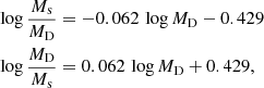
which do not depend on the redshift. However, since Eq. (12) in which the ratio m(MD, z) is used contains its own dependence on the redshift, the final results still depend on this important parameter.
Appendix B: Hydrodynamical models of ETGs
B.1. The pure monolithic scheme
Chiosi & Carraro (2002), by means of hydrodynamical simulations, incorporating radiative cooling, star formation, energy feedback, and chemical evolution, addressed the problem of the formation and evolution of ETGs (from dwarf to normal/giant systems) in the framework of the SCDM cosmological model of the Universe and monolithic scheme of galaxy formation. The cosmological parameters were H0 = 65 km s−1 Mpc−1, a Baryonic-to-dark matter ratio of 1–9, that is, for MT = MB + MD, MB = 0.1MT, MD = 0.9MT, and the redshift at which galaxies were supposed to start the collapse (zf ≃ 1 and zf ≃ 5). A lump of mass (perturbation) with spherical symmetry whose density exceeds a critical value is allowed to collapse toward the virial condition. A Monte Carlo procedure is adopted to fix the initial coordinates and velocities of the DM and BM particles. Table B.1 summarises the key parameters and the results of the models. The key results of this study are as follows:
Summary of the properties of the hydrodynamical model galaxies by Chiosi & Carraro (2002).
(i) The duration, strength, and shape of the star formation rate as a function of time strongly depend on the galaxy mass and the initial density: (a) Galaxies of high initial density and total mass over a wide range undergo a prominent initial episode of star formation followed by quiescence. (b) The same applies to high-mass galaxies of low initial density, whereas the low-mass galaxies undergo a series of burst-like episodes that may stretch up to the present. The details of their star formation history are also very sensitive to the value of the initial density.
(ii) The mass turned into stars per unit total mass of the galaxy is nearly constant which means that the engine at work is the same.
(iii) The ratio between the left-over gas and the initial total BM decreases at increasing total mass of the galaxy.
(iv) As a result of star formation in the central core of the galaxy and consequent gas heating, large amounts of gas are pushed to large distances. After cooling, part of the gas falls back towards the central furnace.
(v) Galactic winds occur. In general all galaxies are able to eject part of their gas content into the intergalactic medium. However, the percentage of the ejected material increases at decreasing galaxy mass.
B.2. The hierarchical scheme
Merlin et al. (2010, 2012) used the parallel hydrodynamical code EvoL to produce a number of models for ETGs with different mass and/or initial density (12 cases in total). The models were followed from the epoch of their detachment from the linear regime, i.e. zi ≥ 20, to a final epoch (redshift zf) different from model to model (but with zf ≤ 1). The simulations included radiative cooling down to 10 K, star formation, stellar energy feedback, re-ionising photo-heating background, and chemical enrichment of the interstellar medium. We refer the reader to these latter-cited papers for all the details of the code. The assumed cosmology was the standard ΛCDM, with H0 = 70.1 km s−1 Mpc−1, flat geometry, ΩΛ = 0.721, σ8 = 0.817; the baryonic fraction ≃0.1656.
Each model starts as a sphere cut at certain redshift zi from a wider cosmological simulation in which density fluctuations exist. At the centre of the sphere there is a peak of given density contrast with respect to the cosmological background. The density contrast is measured by the quantity [δρ1] = [(⟨ρ⟩−ρb)/ρb], where ⟨ρ⟩ is the mean density of the perturbation and ρb the density of the background. The central density peak has a given total mass MT, sum of the DM and BM components. This is the proto-halo of our model galaxy in which stars will be formed at later times. The cosmological simulation provides the initial positions and velocities of all the particles in the proto-halo. An outward radial component is added to the velocity of each particle to take the expansion of the Universe into account. The initial conditions are set in such a way that each model is a re-scaled version of a single reference proto-galactic halo, with different total mass and/or initial over-density. The proto-galactic halos are then followed through their early stages of expansion caused by the Hubble flow, turn around, and collapse. The redshift at which the collapse begins varies from model to model and inside the same model from the centre to the outer regions. In general, the collapse occurs during the redshift interval 4 > z > 2, it starts first in the central regions and gradually moves outwards. The collapse is complete at redshift z ≃ 2. All the models develop a central stellar system, with a spheroidal shape. Massive halos (MT ≃ 1013 M⊙) experience a single, intense burst of star formation (with rates ≥103 M⊙ yr−1) at early epochs, consistently with observations, with a less pronounced dependence on the initial over-density; intermediate mass halos (MT ≃ 1011 M⊙) have SFHs that strongly depend on their initial over-density, i.e. from a single peak to a long lasting period of activity with strong fluctuations in the rate; finally low-mass halos (MT ≃ 109 M⊙) always have fragmented histories resulting in multiple stellar populations, which is due to the so-called “galactic breathing” phenomenon. This confirms the correlation between the initial properties of the proto-halos and their SFHs already found by Chiosi & Carraro (2002). The models have morphological, structural, and photometric properties comparable to real galaxies, in general closely matching the observed data (see Merlin et al. 2012, for all other details). These models can be classified as early hierarchical because they undergo repeated episodes of mass accretion of sub-lumps of matter inside the original density contrast in very early epochs and essentially evolve in isolation thereafter. These reference models are calculated adopting a star formation efficiency of ϵsf = 1. This value is larger than current estimates from observational data in the Local Universe, i.e. ϵsf ≃ 0.025 (Lada & Lada 2003; Krumholz & Tan 2007), and theoretical considerations on the global star-to-total mass ratio in galaxies that suggest ϵsf ≤ 0.1. However, adopting a high value of ϵsf allows for a strong reduction of the computational time, while preserving the basic properties of the models (for a complete discussion see Merlin et al. 2012). The properties of all computed model galaxies are listed in Table B.2.
Early hierarchical galaxy models by Merlin et al. (2010, 2012).
Using the same numerical code and approach for the initial conditions, Chiosi et al. (2012) produced a group of ancillary models, whose initial parameters and key results are listed in Table B.3. These models are calculated to explore the consequences of much higher initial density contrasts and/or lower star formation efficiencies ϵsf. The effect of the higher initial density is already known from the old calculations by Chiosi & Carraro (2002) and the models by Merlin et al. (2012): galaxies of the same mass will be shifted on the MR plane to smaller radii.
Ancillary models of Chiosi et al. (2012).
As expected, by decreasing the efficiency ϵsf, star formation is delayed or even inhibited. The gas continues to flow into the gravitational potential well until the threshold density for star formation to occur is reached and /or a sufficient number of stars are formed. The newly born galaxy is of much smaller dimension with respect to the corresponding object with higher efficiency of star formation.
All the ancillary models are calculated as limited to the very early evolutionary stages in order to show in the MR plane the initial position of a model galaxy in which the gas content has reached densities much higher than the formal mean background density fixed by cosmology. The parameter fδ indicates the factor by which the initial density of the same model in the first group (Table B.2) is scaled. As already mentioned, in these models we also change the efficiency of star formation ϵsf as indicated in Table B.3. In a few models, indicated by ϵZ, the efficiency of star formation increases with metallicity Z. The efficiency goes from ϵsf = 0.1 for Z = 0.0001 to ϵsf = 1 for Z = 0.01 (close to the solar value). This relation has no special meaning, it is simply meant to evaluate the effect of star formation efficiency increasing with metallicity. In any case, this effect plays a marginal role in the position of the model galaxies on the MR plane; see the entries of Table B.3.
All Tables
Coefficients of the relationships log(MD/Ms) = (1−α) log MD − β at different redshifts.
Efficiency of the star formation in galaxies of different mass observed at redshift z = 0.
Summary of the properties of the hydrodynamical model galaxies by Chiosi & Carraro (2002).
All Figures
|
Fig. 1. log(Rs) vs. log(Ms) relation for all the samples under consideration. Rs is the half-mass radius and Ms the total stellar mass. Although Rs is not strictly identical to the effective radius Re, they are very close to each other. Throughout this paper we always use Rs, which is easier to calculate for hydrodynamic models of galaxies, and assume Rs ≃ Re. Burstein et al. (1997) sample: filled red circles are the ETGs, green open circles the SGs, blue filled triangles the DGs, filled red squares the GCs, and filled light-blue squares are the GCGs. The blue dashed line is the linear best fit of Eq. (2), i.e. log Rs = 0.60 log Ms − 5.859 relative to the sole ETGs, but extended to the regions of GCs and GCGs. Bernardi et al. (2010) sample: only ETGs are present, indicated by green filled circles. They fully overlap the ETGs of Burstein et al. (1997). The dashed magenta line is the linear best fit of the ETG data, but extended to GCs and GCGs. WINGS sample: dark-red filled circles are the ETGs, blue filled circles the BCGs, and the black filled circles are the GCGs. The olive-green dashed line is the linear best-fit of all WINGS objects together log Rs = 0.901log Ms − 9.245, but extended to DGs and GCs. Dwarf galaxies and Globular Clusters: coral filled circles are the DGs of Woo et al. (2008) and Geha et al. (2006) all together. Finally, the parallelogram shows the area occupied by the transition objects from GCs to DGs of Kissler-Patig et al. (2006). |
| In the text | |
|
Fig. 2. Left panel: Ms − MD relations at different redshifts (z = 4, blue; z = 2, green; z = 1, yellow; z = 0, red). Masses are in solar units. The solid lines are the best fits, the coefficients of which are given in Table 1. Right panel: same as in the left panel but for the Rs − RD relations. Radii are in kiloparsecs. |
| In the text | |
|
Fig. 3. Stellar half-mass radius Rs vs. mass Ms of the galaxy models of the Illustris database at different redshifts: z = 4 (blue), z = 2 (green), z = 1 (yellow), and z = 0 (red). |
| In the text | |
|
Fig. 4. Evolution of Illustris galaxies on the Rs versus Ms plane from z = 4 to z = 0. There are eight values of redshift along each line. The position of each galaxy at each redshift is marked by a point of different colour. The colour code is as follows: blue (z = 4.0), medium-blue (z = 3.0), light-green (z = 2.2), green (z = 1.6), cyan (z = 1.0), magenta (z = 0.6), coral (z = 0.2), and red (z = 0). The solid lines are the best fits of the Illustris data for z = 0 in the domain of massive galaxies MT ≥ 1011 M⊙ (red), and of the Bernardi et al. (2010) ETGs by Chiosi et al. (2012; green). Here we show 20 cases randomly chosen from the whole sample. |
| In the text | |
|
Fig. 5. Same as Fig. 3 but limited to the sample for z = 0 for all models with zero star formation rate. |
| In the text | |
|
Fig. 6. Composite Rs-versus-Ms relation and comparison between theory and observations. The light powder-blue dots are the data of Burstein et al. (1997) for ETGs, DGs, GCs, and GCGs, and the dashed line of the same colour is the best fit of the sole ETGs, this time extended to the domains of GCs and GCGs. The bright green dots are the Bernardi et al. (2010) data for ETGs, and the thick dashed line of the same colour is the best-fit line of these latter. The red, blue, and green-blue dots are the ETGs, BCGs, and GCGs of the WINGS sample. The dashed red line is the best-fit line of the ETGs, whereas the solid blue line is the best fit of all WINGS data lumped together. The slope of this latter line is very close to the MRR for virialised objects. In this case the line fails to hit the region of GCs. Finally, we display different theoretical models for comparison. The black filled squares connected by the black solid line and the red squares connected by the solid red line are the monolithic models by Chiosi & Carraro (2002) and their linear fit. The two groups of models differ for the density of the Universe (redshift) at initial collapse. The three coral open circles are low-mass ETGs with the same mass but slightly different initial densities by Chiosi & Carraro (2002); see the data of Table B.2. The empty red star is the merger reported by Chiosi & Carraro (2002). The blue squares connected by the blue line are the hierarchical models by Merlin et al. (2010, 2012); see Table B.3 for more details. The light blue-green squares are the ancillary model of Chiosi et al. (2012); see Table B.3. Finally, the dark olive-green points are the reference model galaxies of the Illustris simulations. |
| In the text | |
|
Fig. 7. Comparison of the Fan et al. (2010) lines and the theoretical models by Merlin et al. (2012; green filled squares) with the observational data of Burstein et al. (1997) from GCs (small red squares), to DGs (small blue triangles), and GCGs (light blue filled circles) plus the ETGs of Bernardi et al. (2010; red dots). The short-dashed blue line is the Fan et al. (2010) relation for z = 0. The thin solid lines of different colours are the same relation but for z = 1, z = 5, z = 10, z = 15, and z = 20 from top to bottom in the order. The long-dashed, thick blue line is the best-fit of the ETGs of Bernardi et al. (2010) extended to GCs and GCGs. |
| In the text | |
|
Fig. 8. Growth function of halos n(MD, z) reproduced from Lukić et al. (2007). |
| In the text | |
|
Fig. 9. Cosmic galaxy shepherd and the corresponding locus of DM parent halos (the black solid thick and thin lines, respectively) for the number density of Ns = 10−2 halos per (Mpc h−1)3. In addition to this we show the case with Ns = 10−8 halos per (Mpc h−1)3 (the magenta solid thick and thin lines). The various loci are plotted onto the observational MR plane (see text for all details). We also draw the observational data for the sample of Bernardi et al. (2010) with the linear fit obtained by these latter authors, and two theoretical MRRs from Eq. (12) of (Fan et al. 2010; solid thin blue lines) relative to z = 0 and z = 10, with m = 15 and fσ = 1. In addition to this, the present-day position of the reference galaxy models and their linear fit are shown (the golden filled squares and solid line). Finally, the filled black squares and magenta circles show the cosmic galaxy shepherd at different redshifts (z = 0, 1, 5 10, 15, and 20) for the two cases of the number density per (Mpc h−1)3. |
| In the text | |
|
Fig. 10. Mass-radius relationship: comparison between data and theory. Radii Rs and stellar masses Ms are in kiloparsecs and M⊙, respectively. The pale-blue filled circles are all the data considered in this study, and the pale green filled circles are the models of Illustris. The dark-red thick crossed line is the linear best fit of normal ETGs (MT ≥ 1010 M⊙) given by Eq. (3), but prolonged down to the region of GCs and upwards to that of GCGs. The four solid dashed line labelled Mod-A (zf = 5, blue), Mod-B (zf = 1, red and zf = 2, dark green), and Mod-C (zf = 10 black) are the analytical relationships of Eq. (34) showing the loci of galaxy models with different mass but constant initial density for different values of redshift of galaxy formation zf as indicated. These lines are the best fit of the models by Chiosi & Carraro (2002), Merlin et al. (2012), and Chiosi et al. (2012); see Tables B.1–B.3. The magenta solid lines show the virial condition on the MR plane for different velocity dispersion (50, 250 500 km s−1 from left to right). The dashed black lines labeled by different values of zf are the MRRs expected for galaxies with total mass equal to 50 × MCO(z), the cut-off mass of the Press-Schechter at varying zf according to relation (35). These lines go in pairs with the best-fit lines of models of identical initial density labelled with the same colour. The large empty squares illustrate the intersections between the lines of constant initial density and the MRRs for 50 × Mco galaxies for equal redshift. All the intersections lie very close to the relation of Eq. (3) shown by the dark-red crossed line. This is the linear interpretation of the observed MRR, i.e. the analytical demonstration of Sect. 5. Finally, the curved blue dotted line shows the expected MRR for the baryonic component of DM halos whose mass distribution follows the cosmological HGF by Lukić et al. (2007). The curve has been extended to include the GCs and the GCGs (see main text for more details). We highlight the ever changing slope of the MRR which decreases passing from GCGs to ETGS and GCs. Remarkably, the curved line first runs very close to the large empty squares, and then secondly to a linear fit of the data (crossed line), and third accounts for the observed MRR passing from GCs to GCGs (about ten orders of magnitude difference in star mass). The horizontal blue line shows the interval for Ms corresponding to initial masses MCO(z) < MT < 10 × MCO(z) (the percentage of galaxies in this interval amounts to ≃15%), which highlights the fact that at each redshift the high-mass edge of the MRR has a natural width. |
| In the text | |
|
Fig. 11. log[Rs] vs. log[Ms] relation for compact galaxies (filled blue circles) and their best fit (blue dashed line). The red open circles are the ETGs from Bernardi et al. (2010) plotted here for comparison, and the red dashed line is their best-fit. The large filled circles are the 12 ancillary models (black the efficiency of star formation ϵsff = 1, green for ϵsff = 0.5, and red for ϵsff = 0.1). The thin straight lines are the present-day MRRs of model galaxies that started their collapse at different redshifts, namely zf = 1, zf = 5, zf = 8, and zf = 10 from top to bottom. The lines are given by Eq. (34). |
| In the text | |
|
Fig. A.1. Relations Ms/MDMD at different redshifts for theoretical models (all masses are in solar units). The dotted lines of different colours correspond to the eight values of the redshift z = 0 and z = 0.2 (top, red), z = 0.6, z = 1.0 (intermediate, yellow), z = 1.6 and z = 2.2 (intermediate, green), z = 3 and to z = 4 (bottom, blue). The black dots are the values predicted by Eq. (A.1) at varying log MD from 4 to 14 in steps of 1 and redshift z from 0 to 4 in steps of 1, respectively. The large red and golden circles are the combination of Eqs. (A.3) and (A.2), respectively. The open magenta (z = 0) and black (z = 3.95) circles are relation Ms/MD vs. MD at different redshifts according to Girelli et al. (2020). We note how all relations agree with each other at log MD ≃ 12 whereas they badly disagree at lower values of MD. |
| In the text | |
Current usage metrics show cumulative count of Article Views (full-text article views including HTML views, PDF and ePub downloads, according to the available data) and Abstracts Views on Vision4Press platform.
Data correspond to usage on the plateform after 2015. The current usage metrics is available 48-96 hours after online publication and is updated daily on week days.
Initial download of the metrics may take a while.