| Issue |
A&A
Volume 643, November 2020
|
|
|---|---|---|
| Article Number | A178 | |
| Number of page(s) | 19 | |
| Section | Interstellar and circumstellar matter | |
| DOI | https://doi.org/10.1051/0004-6361/202037659 | |
| Published online | 20 November 2020 | |
Ammonia observations towards the Aquila Rift cloud complex
1
Xinjiang Astronomical Observatory, Chinese Academy of Sciences,
830011
Urumqi,
PR China
e-mail: This email address is being protected from spambots. You need JavaScript enabled to view it.
; This email address is being protected from spambots. You need JavaScript enabled to view it.
2
University of Chinese Academy of Sciences,
100080
Beijing,
PR China
3
Key Laboratory of Radio Astronomy, Chinese Academy of Sciences,
830011
Urumqi,
PR China
4
Max-Planck-Institut für Radioastronomie,
Auf dem Hügel 69,
53121
Bonn,
Germany
e-mail: This email address is being protected from spambots. You need JavaScript enabled to view it.
5
Astronomy Department, King Abdulaziz University,
PO Box 80203,
21589
Jeddah,
Saudi Arabia
6
Department of Solid State Physics and Nonlinear Physics, Faculty of Physics and Technology, AL-Farabi Kazakh National University,
050040
Almaty,
Kazakhstan
Received:
4
February
2020
Accepted:
23
September
2020
Abstract
We surveyed the Aquila Rift complex including the Serpens South and W 40 regions in the NH3 (1,1) and (2,2) transitions making use of the Nanshan 26-m telescope. Our observations cover an area of ~ 1.5° × 2.2° (11.4 pc × 16.7 pc). The kinetic temperatures of the dense gas in the Aquila Rift complex obtained from NH3 (2,2)/(1,1) ratios range from 8.9 to 35.0 K with an average of 15.3 ± 6.1 K (errors are standard deviations of the mean). Low gas temperatures are associated with Serpens South ranging from 8.9 to 16.8 K with an average of 12.3 ± 1.7 K, while dense gas in the W 40 region shows higher temperatures ranging from 17.7 to 35.0 K with an average of 25.1 ± 4.9 K. A comparison of kinetic temperatures derived from para-NH3 (2,2)/(1,1) against HiGal dust temperatures indicates that the gas and dust temperatures are in agreement in the low-mass-star formation region of Serpens South. In the high-mass-star formation region W 40, the measured gas kinetic temperatures are higher than those of the dust. The turbulent component of the velocity dispersion of NH3 (1,1) is found to be positively correlated with the gas kinetic temperature, which indicates that the dense gas may be heated by dissipation of turbulent energy. For the fractional total-NH3 (para+ortho) abundance obtained by a comparison with Herschel infrared continuum data representing dust emission, we find values from 0.1 ×10⁻⁸ to 2.1 ×10⁻⁷ with an average of 6.9 (±4.5) × 10−8. Serpens South also shows a fractional total-NH3 (para+ortho) abundance ranging from 0.2 ×10⁻⁸ to 2.1 ×10⁻⁷ with an average of 8.6 (±3.8) × 10−8. In W 40, values are lower, between 0.1 and 4.3 ×10⁻⁸ with an average of 1.6 (±1.4) × 10−8. Weak velocity gradients demonstrate that the rotational energy is a negligible fraction of the gravitational energy. In W 40, gas and dust temperatures are not strongly dependent on the projected distance to the recently formed massive stars. Overall, the morphology of the mapped region is ring-like, with strong emission at lower and weak emission at higher Galactic longitudes. However, the presence of a physical connection between the two parts remains questionable.
Key words: surveys / radio lines: ISM / ISM: molecules / ISM: kinematics and dynamics / stars: formation
© ESO 2020
1 Introduction
Systematic studies of dense molecular cores in regions of high-mass-star formation (HMSF) are of great importance for our understanding of their physical and chemical properties. In comparison with low-mass star-forming regions, only a few, rather arbitrarily selected cores associated with HMSF regions have been investigated in some detail (Zinnecker & Yorke 2007; Tan et al. 2014). There is a clear observational dichotomy between low-mass-star formation (LMSF) and HMSF. It is suggested that more than 70% of HMSF stars are formed in dense clusters embedded within giant molecular clouds (GMCs; Lada & Lada 2003). For a better understanding of massive star formation, it is important to obtain the physical conditions of HMSF regions. High-mass stars form almost exclusively in GMCs while low-mass stars can form in dark clouds as well as in GMCs. High-mass stars are predominantly formed in clusters, while low-mass stars may form in smaller molecular complexes as for example in the Taurus molecular cloud or in isolation. The star formation efficiency is generally higher in HMSF regions (e.g., Myers et al. 1986; Lada & Lada 2003). In HMSF regions, densities and temperatures tend to be higher, and spectral line widths are larger indicating a higher degree of turbulence. However, the causal relationship between the presence of young high-mass stars, molecular cloud characteristics, and details of the star formation process is not well established.
The star formation region in the Aquila Rift is located at a distance of ~436 ± 9.2 pc (e.g., Ortiz-León et al. 2017, 2018) in areas extending up to Galactic latitudes of at least + 10° and down to −20° (e.g., Dobashi et al. 2005). The Aquila Rift contains several active star-forming regions: Serpens Main, Serpens South, Serpens MWC297, and W 40. Here, we focus on that part of the Aquila Rift complex that harbors two known sites of star formation: Serpens South and W 40. Serpens South is a well-known site of star formation located in the western part of the Aquila Rift cloud complex and forms a young embedded stellar cluster (Gutermuth et al. 2008). It has a filamentary structure on the cusp of a burst of LMSF. W 40, located further to the east in equatorial coordinates, is a site of ongoing HMSF. It still contains dense molecular cores (Dobashi et al. 2005) and includes a blistered H II region, powered by a compact OB association that contains pre-main sequence stars (e.g., Zeilik & Lada 1978; Smith et al. 1985; Vallee 1987; Kuhn et al. 2010; Rodríguez et al. 2010; Mallick et al. 2013).
Aquila is a unique region for studying the physical and chemical conditions of molecular clouds. A large number of molecular line observations have been performed, such as in CO (Nakamura et al. 2017; Su et al. 2019, 2020), in NH3 (Levshakov et al. 2013, 2014; Friesen et al. 2016)and in H2CO (Komesh et al. 2019). This was complemented by SCUBA-2 450 and 850 μm observations(Rumble et al. 2016). A few years ago, the whole Aquila complex was extensively studied by the Herschel Gould Belt Survey1 , yielding more than 500 detections of starless cores imaged in dust emission at 70–500 μm (Könyves et al. 2010). However, a systematic spectral survey of the dense gas in the region covering and comparing the emission of both Serpens South and the W 40 complex is still missing. A basic result of the NH3 studies of Levshakov et al. (2013, 2014), mostly carried out in position-switching mode, was that they were often finding unknown clouds at the OFF positions, providing the urgent need for a systematic survey of the entire region. Friesen et al. (2016) presented NH3 measurements of Serpens South (~4 pc × 4 pc) with the Green Bank Telescope (GBT). Here we present a complementary survey with lower angular resolution but a twelve-times-larger area encompassing many Aquila rift clouds with substantial visual extinction.
Ammonia (NH3) is frequently used as the standard molecular cloud thermometer (e.g., Ho & Townes 1983; Walmsley & Ungerechts 1983; Danby et al. 1988); it starts to form at an early stage of prestellar core evolution and becomes brightest during the later stages (e.g., Suzuki et al. 1992). NH3 (1,1) and (2,2), both belonging to the para-species of ammonia, have proven to form an excellent thermometer at Tkin < 40 K (Walmsley & Ungerechts 1983). They can also serve as a good thermometer for higher temperatures after some modification of the rotational temperature but with a reduction in precision (Walmsley & Ungerechts 1983; Danby et al. 1988; Tafalla et al. 2004). Moreover, the critical densities of NH3 (1,1) and (2,2) are about 103 cm−3 (Evans 1999; Shirley 2015), thus providing a proper tracer for dense regions.
In this paper we intend to provide novel ammonia maps covering the entire region of the Aquila Rift cloud complex and to reveal a complete distribution of the dense gas. The article is organized as follows: in Sect. 2 we introduce our observations and data reduction. Results are highlighted in Sect. 3. We discuss the variation of NH3 abundance and gas temperature in Sect. 4. Our main conclusions are summarized in Sect. 5.
2 Observations and data reduction
2.1 NH3 observations
From March 2017 to August 2018, we observed the NH3 (1,1) and (2,2) lines with the Nanshan 26-m radio telescope. A 22.0–24.2 GHz dual polarization channel superheterodyne receiver was used. The main parameters of the Nanshan telescope and survey area are listed in Table 1. The rest frequency was centered at 23.708 GHz to observe NH3 (1,1) at 23.694 GHz and (2,2) at 23.723 GHz simultaneously. To convert antenna temperatures  into main beam brightness temperatures TMB, a beam efficiency of 0.59 was adopted. The observations were calibrated against periodically (6 s) injected signals from a noise diode. We observed IRAS 0033+636 (α = 00:36:47.51, δ = 63:29:02.1, J2000) repeatedly during observations (Schreyer et al. 1996), adopting a main beam brightness temperature TMB = 4.5 K. Systematic variations and dispersion of brightness temperatures are small (see Appendix A). The standard deviation of the mean is ~ 10% (see Fig. A.1). To further check our calibration stability, we compared our NH3 data with previously taken NH3 data observed with the GBT in Fig. A.2 (Sokolov et al. 2017). The two data sets obtained from G035.39-0.33 are in good agreement.
The typical system temperature was ~50 K ( scale) at 23.708 GHz. The map was made using the on-the-fly (OTF) mode with a 6′ × 6′ grid size and 30′′ sample step. All observations were obtained under excellent weather conditions and above an elevation of 20°. The mapped region was divided into six areas (see Fig. 1). The main parameters of each area are listed in Table A.1. The whole map covers a region of ~ 1.5° × 2.2° (11.4 pc × 16.7 pc).
Main parameters of the Nanshan telescope and survey area.
2.2 Data reduction
The CLASS and GREG packages of GILDAS2, and also python plot packages matplotlib (Hunter 2007) and APLpy3 were used for all the data reduction. The spectra were resampled in steps of ~1′. To enhance signal-to-noise ratios (S/Ns) in individual channels, we smoothed in many but not all cases (see Sect. 3.1) contiguous channels to a velocity resolution of ~0.2 km s−1. A typical rms noise level (1σ) is ~0.03–0.05 K (TMB scale) for a channel of ~0.2 km s−1 in width (see Table A.1). With respect to NH3 , we chose two fitting methods: “GAUSS” fitand NH3 (1,1) fit. In orderto convert hyperfine blended line widths to intrinsic line widths in the NH3 inversion spectrum (e.g., Barranco & Goodman 1998), we also fitted the averaged spectra using the GILDAS built-in “NH3 (1,1)” fitting method which can fit all 18 hyperfine components simultaneously. From the NH3 (1,1) fit we can obtain integrated intensity, line center velocity, intrinsic line widths of individual hyperfine structure (hfs) components, and optical depth. Main beam brightness temperatures TMB are obtained from GAUSS fit. These fitting methods were also used in previous works, such as by Wienen et al. (2012) and by Wu et al. (2018). Examples for reduced and calibrated spectra of NH3 (1,1) and (2,2) inversion lines are given in Fig. 2.
Because the hyperfine satellite lines of the NH3 (2,2) transition are mostly weak, NH3 (2,2) optical depths are not determined. A single Gaussian profile was fitted to the main group of NH3 (2,2) hyperfine components. Physical parameters of dense gas such as rotational temperature (Trot), kinetic temperature (Tkin), and para-NH3 column density ( were derived using the method described by Ho & Townes (1983) and Ungerechts et al. (1986) (see Sects. 3.2 and 3.3).
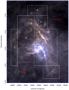 |
Fig. 1 Color image of the Aquila Rift (red for 500 μm, green for 350 μm, and blue for 250 μm, all derived from Herschel data; Bontemps et al. 2010; Könyves et al. 2010). The regions subsequently observed in NH3 are marked by six boxes (see Table A.1). |
3 Results
3.1 NH3 distribution
NH3 (1,1) and (2,2) velocity-integrated intensity maps of the main groups of hyperfine components are presented in Fig. 3. Intensities were integrated over the Local Standard of Rest velocity (VLSR) range of 4–10 km s−1. NH3 (1,1) shows an extended distribution and clearly traces the dense molecular structure including Serpens South and W 40. NH3 (2,2) is only detected in the densest regions of Serpens South and W 40, and shows a much less extended distribution.
What we find in Fig. 3 is an Aquila Rift morphology that resembles the Herschel color infrared image shown in Fig. 1 in many aspects, but also shows clear differences (see also Fig. 1 of Könyves et al. 2010 for an H2 column density map of the region, based on Herschel data). In the Serpens South region, there is a dominant ridge of strong NH3 (1,1) emission from the southwest to the northeast (position angle ~30° in Galactic coordinates) containing several cores with a total length of about 15′. This is also seen in the color Herschel infrared image, but the latter is dominated by relatively hot dust associated with the W 40 complex, where NH3 emission is present at a lower level. Weaker NH3 emission extending further to the south and north follows the color Herschel infrared image. Our mapped area with highest Galactic longitudes, region 5 in Fig. 1, showing only weak emission, is also seen in our NH3 (1,1) map. Overall, the NH3 distribution (Fig. 3) shows a ring-like morphology, with the center of this ring located in region 4 (see Fig. 1 and Sect. 4.5). With a radius of 25′ –30′ (about 3.5 pc) it is roughly circular and exhibits comparatively strong dust and NH3 emission at its low and weak emission at its high Galactic longitude side.
Previous SPIRE/PACS observations from the Herschel Gould Belt survey towards the Aquila cloud complex (Könyves et al. 2015) identified 446 candidate prestellar cores and 58 protostellar cores in the Aquila region. Using this catalog, we find 362 prestellar cores and 49 protostellar cores in our observed area and show their distribution in Fig. B.1. The two data sets of pre- and protostellar cores on the one side and the NH3 data on the other match each other very well. All protostellar cores are associated with regions of notable (>0.13 K km s−1) NH3 emission, while prestellar cores are even found in the weak high-longitude region of the large ring-like structure.
Using the “NH3(1,1)” fit procedure (see Sect. 2.2), the NH3 (1,1) intensity-weighted mean velocity (moment 1) and velocity dispersion (moment 2) maps are presented in Fig. 4. These maps visualize the kinematics of the Aquila Rift derived from NH3 (1,1). The two images are overlaid with NH3 (1,1) integrated intensity contours as in Fig. 3. Here we use a higher threshold of 5σ for the lowest contours to provide reliable results. Previous NH3 observations with the GBT (beam size ~30′′; Friesen et al. 2016) toward the Serpens South indicated narrow line widths, typically of order 0.5 km s−1, but with minima near 0.15 km s−1, and therefore in this case we used a velocity resolution of 0.1 km s−1 to fit the NH3 spectral lines. The intensity-weighted mean velocity map (see Fig. 4 left panel) reveals that the mg of hf components shows a velocity range from 4.5 to 8.4 km s−1. The dominant ridge of NH3 emission mostly indicates velocities in excess of 7 km s−1. Only at its southern edge and to the west of its northern edge velocities are smaller (see also Fig. 4 of Friesen et al. 2016). Velocities in regions 5 and 6 cannot be shown because the S/Ns are low. In these regions with weak NH3 (1,1) line emission we obtain averaged radial velocities of 8.2 ± 0.8 and 7.1 ± 0.5 km s−1, respectively,which is consistent with those encountered in the regions with stronger emission.
From the FWHM line-widths (moment 2) map (see Fig. 4 right panel) we can see that the small region with widest lines is located in the northwest of Serpens South, while another small spot with relatively high dispersion is encounteredin the south. Elsewhere, rather low and also uniform intrinsic (for individual hf components) dispersions (σ ~ 0.5 km s−1) are present. Irregular and larger dispersions are obtained in region 2 (see Fig. 1 for location and extent of this region).However, this may be merely a consequence of low S/Ns. We study the FWHM line widths of the NH3 (1,1) main lines with a peak line flux threshold of 5σ as summarized in Fig. 5a. The line width refers to the individual hf components. The line width distribution of the NH3 (1,1) gas appears to have an outstanding peak around 0.5 km s−1, which is inagreement with the findings of Friesen et al. (2016).
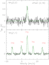 |
Fig. 2 NH3 (1,1) and (2,2) spectra at offset (Δl, Δb) = (2′, 16′) with respect to the reference position (l = 28.59°, b = 3.55°). In each panel, the black solid line represents the observed spectrum, the green solid line indicates the NH3 (1,1) fitting (lower panel) and Gaussian fitting (upper panel) of the NH3 (2,2) line (see Sect. 2.2). The groups of hyperfine components “mg”, “isg”, and “osg” represent the main, inner-satellite, and outer-satellite groups. The velocity scale is Local Standard of Rest, here and elsewhere. |
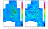 |
Fig. 3 Integrated intensity maps of NH3 (1,1) (left) and (2,2) (right). The reference position is l = 28.59°, b = 3.55°. The integration range is 4 < VLSR < 10 km s−1. Contours start at 0.13 K km s−1 (3σ) on a main beam brightness temperature scale and go up in steps of 0.13 K km s−1. The unit of the color bars is K km s−1. The half-power beam width is illustrated as a black filled circle in the lower left corners of the images. The red line in the top right of each map illustrates the 1 pc scale at a distance of 436 pc (Ortiz-León et al. 2017, 2018). Left panel: black stars show the positions of the identified 38 ammonia clumps (see Sect. 3.2). |
3.2 Dense clump identification
Based on the distribution of the integrated intensity of the NH3 (1,1) line in Fig. 3, we use the Clumpfind2d algorithm (Williams et al. 1994) to identify dense core clumps. First, the root mean square of the integrated intensity map was derived based on a background noise estimate of 0.04 K in a 0.2 km s−1 wide channel from regions with weak emission. The level range from a threshold of 5 to 37σ was then set with increments of 4σ (where σ is the rms noise level). Within the integrated intensity map, 38 potential dense clumps associated with the Aquila Rift were identified after eliminating a fake clump located at the boundary of the map. In order to further confirm the authenticity of the condensations identified by Clumpfind2d, we also tried different parameter settings and found that the location of the dense clumps remained the same and also that many false structure results appeared when using a lower threshold of ≤ 3σ. Adopting the output from the Clumpfind2d algorithm, it should be noted that the clumps identified around Aquila are located mostly along the dominant NH3 ridge with some additional sources further in the north and south (see Fig. 3). The black stars in Fig. 3 (left panel) show the positions of the identified 38 clumps. Among these 38 clumps both NH3 (1,1) and (2,2) emission lines are detected in 17 clumps. Observed parameters and calculated model parameters are given in Tables B.1–B.3. NH3 (1,1) and (2,2) spectral lines towards the 17 clumps are shown in Fig. B.2. For the other 21 clumps NH3 (1,1) spectra are shown in Fig. B.3. Clumps are closely associated with pre- and protostellar cores. While all protostellar cores appear near the clumps, the prestellar cores exhibit a more widespread distribution (see also Fig. B.1 and Sect. 3.1).
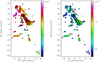 |
Fig. 4 Para-NH3 (1,1) intensity-weighted mean velocity (moment 1, left) and FWHM line width (moment 2, right) maps. The reference position is l = 28.59°, b = 3.55°. These intensity-weighted mean velocities and FWHM line widths referring to the individual hf components are derived from the GILDAS built-in “NH3 (1,1)” fitting method (Sect. 2.2). The considered velocity range is 4 < VLSR < 10 km s−1 for each panel. Contours of integrated intensity start at 0.23 K km s−1 (5σ) on a main beam brightness temperature scale and go up in steps of 0.23 K km s−1. |
3.3 Kinetic temperature
The relative population of the K = 1 and 2 ladders of NH3 are highly sensitive to collisional processes because they are not directly connected radiatively. This allows us to use them as a thermometer of the gas kinetic temperature. We obtained the rotation temperature of NH3 (1,1) and (2,2) using the method described in Ho & Townes (1983), which is
 (1)
(1)
where τm is the peak optical depth of the (1,1) main group of hf components derived using the GILDAS built-in “NH3 (1,1)” fitting method. The main beam brightness temperatures TMB of the (1,1) and (2,2) inversion transitions were derived using the GILDAS built-in “GAUSS” fitting. A histogram of the peak optical depth of the (1,1) main group of hyperfine components, τm (1, 1), for those positions with NH3 (1,1) S∕N > 5σ is summarized in Fig. 5b. The optical depth distribution of the NH3 (1,1) gas peaks around 1.2. The NH3 (1,1) main beam brightness temperatures (TMB < 2 K) are higher than those of the NH3 (2,2) line (TMB < 0.5 K), meaning that the NH3 (2,2) lines can be considered to be optically thin.
In the most prominent regions, where both the NH3 (1,1) and (2,2) lines were detected at levels of at least 5σ, the rotational temperature lies between 8.6 and 25.3 K with an average of 13.4 ± 4.1 K (errors are standard deviations of the mean throughout the article). The median and mean values are 11.8 and 13.4 K, respectively. The statistical distribution of Trot is summarized in Fig. 5c and shows a typical value of about 10 K.
Following Tafalla et al. (2004) to connect rotational with kinetic temperatures, we used
 (2)
(2)
where the energy gap between the (1,1) and (2,2) states is ΔE12 = 42 K. Tafalla et al. (2004) ran different Monte Carlo models involving the NH3 (J, K) = (1,1), (2,1), and (2,2) inversion doublets and an n(r) =  density distribution to compare their observationally determined approximately constant rotational temperatures with modeled kinetic temperatures in dense quiescent molecular clouds. Equation (2) is derived from fitting Tkin in the range of 5 to 20 K, and most of our sources can be found in this interval.
The kinetic temperatures of the dense gas in the Aquila Rift complex obtained from NH3 (2,2)/(1,1) ratios wherever the (2,2) line has been detected at a > 5σ level range from 8.9 to 35.0 K with an average of 15.3 ± 6.1 K. The median and mean values are 12.7 and 15.3 K, respectively. The distribution of the NH3 kinetic temperatures is presented in Fig. 5d and shows a typical value of about 12 K.
The gas kinetic temperatures derived from the NH3(2,2)/(1,1) map are shown in Fig. 6, left panel. We find that dense gas temperatures from para-NH3 in Serpens South are predominantly cold ranging from 8.9 to 16.8 K with an average of 12.3 ± 1.7 K, while W 40 at lower Galactic latitudes, which represents a young stellar cluster associated with an H II region, shows values from 17.7 to 35.0 K with an average of 25.1 ± 4.9 K (see Table 1 for the relevant areas representing Serpens South and W 40). The kinetic temperatures in the dense gas around W 40 and in the lower right part of our map are high (~25 K; see Fig. 6 left panel), which is twice higher than that (~12 K) in the LMSF region of Serpens South. For those 21 clumps with only upper limits to the NH3 (2,2) lines (see Sect. 3.2), the resulting upper kinetic temperature limits are ≲ 10 K.
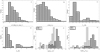 |
Fig. 5 Histograms of physical parameters derived from NH3. (a) Intrinsic FWHM line widths of individual NH3 (1,1) hyperfine structure components with a peak line flux threshold of 5σ; (b) peak optical depths of the main group of hf components τm(1, 1) for those positions with NH3 (1,1) S∕Ns > 5σ (these line widths and peak optical depths are derived from the GILDAS built-in “NH3 (1,1)” fitting method); (c) rotational temperature Trot, where both the NH3 (1,1) and (2,2) lines were detected, at levels of at least 5σ; (d) kinetic temperature Tkin, for those positions with NH3 (2,2) line detections and >5σ features; (e) para and total (para+ortho) column densities of NH3, for those positions exhibiting NH3 (2,2) line detections and >5σ features, assuming an ortho- to para-ratio in thermal equilibrium at the presently obtained kinetic temperature; (f) para-NH3 fractional abundance χ = [para-NH3]/[H2], and total-NH3 (para+ortho) fractional abundance χ = [total-NH3]/[H2], toward the positions with NH3 (2,2) line detections and >5σ features, again adopting ortho- to para NH3 ratios assuming thermal equilibrium. |
3.4 NH3 column density
The total para-NH3 column densities can be calculated from NH3 (1,1), following Wienen et al. (2012)
 (3)
(3)
In many cases the NH3 (1,1) inversion lines are optically thick, and the optical depth is determined by the GILDAS built-in “NH3 (1,1)” fitting method (see Sect. 2.2). The column density in the (1, 1) state is related to the optical depth τtot, according to Mauersberger et al. (1986), by
 (4)
(4)
where N is in cm−2, the FWHM line width Δv is in km s−1, the line frequency ν is in GHz, and the excitation temperature Tex is in Kelvin. In the optically thick case, the excitation temperature Tex is derived from the main beam brightness temperatures TMB and the optical depth τ by
 (5)
(5)
If τ ≪ 1, the main beam brightness temperature TMB is assumed to be Tex τ.
We calculated the ortho-column densities using the ortho- to para-NH3 abundance ratios as a function of Tkin in Fig. 3 of Takano et al. (2002). These were added to the para-column density to get the total (para + ortho) column densities of NH3 (see Tables 2 and B.3).
The conversion between ortho- and para-NH3 is very slow and may take as long as 106 yr (Cheung et al. 1969). As a result, the excitation temperature between the ortho- and para-species, the so-called spin temperature, is often believed to reflect the formation temperature. Assuming thermalization in this sense, the ortho- to para-NH3 ratios are close to unity at Tkin ≳ 30 K, while they can reach values of four at Tkin ~ 10 K (Takano et al. 2002). An even slightly higher range of uncertainty is introduced by detailed models also introducing uncertainties in the poorly known spin temperatures of H2 and NH , which play an essential role in the formation of ammonia. Depending on the detailed circumstances, Faure et al. (2013) find ammonia ortho- to para abundance ratios of ~1.5 and even ~0.7, rather independentof kinetic temperature for values below 30 K. We conclude that the maximum error in our adopted thermalized ortho-to-para NH3 abundance ratios could be a factor of 4.9/0.7 = 7.0, representing a case where we determine Tkin ~ 8.9 K (our lowest kinetic temperature), while the actual ortho- to para-abundance ratio is not 4.9 as expected in case of thermalization, but 0.7 (see Persson et al. 2012). However, even in this worst-case scenario our total NH3 abundance would only be overestimated by half an order of magnitude, that is, by 5.9/1.7 = 3.5. The higher the kinetic temperature, the smaller the uncertainty related to the ortho-NH3 column density correction.
The observed NH3 spectra wereanalyzed in the way described in Eqs. (1)–(5). In addition, detailed derivations of these equations are give in the Appendix of Pandian et al. (2012) and Levshakov et al. (2013). Furthermore, uncertainty estimations of the NH3(1,1) and (2,2) spectra are given in Appendix C.
As can be seen in the central panel of Fig. 6, we provide a total column density map of NH3 for those positions exhibiting NH3(2,2) line detections and >5σ NH3 (1,1) features. The Aquila clumps show a broad distribution of total-NH3 column densities from 0.2 × 10¹⁴ to 6.4 ×1015 cm−2 with an average of 2.1 (± 1.6) × 1015 cm−2. The total-NH3 column density range is 0.3 ×10¹⁴ to 6.4 ×1015 cm−2 with an average of 2.6 (±1.4) × 1015 cm−2 in Serpens South, while in W 40 total NH3 column densities vary from 0.2 to 7.6 ×1014 cm−2 with an average of 2.6 (±2.1) ×1014 cm−2. The distribution of total column densities of NH3 is presented as a histogram in Fig. 5e and has an outstanding peak around 2.4 ×1015 cm−2 seen in our data for Serpens South.
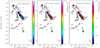 |
Fig. 6 Maps of NH3 kinetic temperature in units of Kelvin (left), the logarithm of the total-NH3 column density in units of cm−2 (middle), and the corresponding logarithm of the fractional abundance (right). The reference position is l = 28.59°, b = 3.55°. Contours of integrated NH3 (1,1) intensity are the same as in Fig. 4 and cover the velocity range 4 < VLSR < 10 km s−1. Contours start at 0.23 K km s−1 (5σ) on a main beam brightness temperature scale and go up in steps of 0.23 K km s−1. Magenta stars show the locations of the OB association (OS1a, IRS1, IRS1a, IRS2, IRS2a, IRS2b, IRS3, and IRS3a) in W 40. |
Parameters obtained from Serpens South and W 40.
 |
Fig. 7 Column densities derived from total-N(NH3) for Serpens South (blue points) and W 40 (red points) vs. N(H2) column densities (left), total column densities of N(NH3) vs. kinetic temperature (middle), and total fractional NH3 abundance, N(total-NH3)/N(H2), vs. kinetic temperature Tkin(NH3) (right). |
4 Discussion
4.1 Variation of NH3 abundance
Measurements of the NH3 abundance in different star-forming regions have shown a large spread, for example 10−5 in dense molecular “hot cores” around newly formed massive stars due to dust grain evaporation (Mauersberger et al. 1987), 10−8 in quiescent dark clouds (Benson & Myers 1983), and 10−9 in the Orion Bar photon-dominated region (PDR; Batrla & Wilson 2003; Larsson et al. 2003) because it is extremely affected by a high UV flux. A few times 10−10 in the LargeMagellanic Cloud (LMC) and in M82 may characterize an environment with low metallicity and a high UV radiation field (Weiß et al. 2001; Ott et al. 2010).
Our total-NH3 column densities N(NH3) are compared with the column densities of H2 derived from the Herschel infrared continuum data representing dust emission (André et al. 2010; Könyves et al. 2015), for which we smoothed the data to our beam size of 2′. The NH3 column densities areconsistent with studies reported towards other Gould Belt star-forming regions (Friesen et al. 2017), where the logarithm of the para-NH3 column density (log N(para-NH3)) varies from 13.0 to 15.5.
The fractional total-NH3 abundance map (χ (total-NH3) = (total-N (NH3))/N(H2)) is shown in the right panel of Fig. 6. The relative total NH3 abundances N(total-NH3)/N(H2) range from 0.1 ×10⁻⁸ to 2.1 ×10⁻⁷ with an average of 6.9(±4.5) × 10−8, and the relative para-NH3 abundances N(para-NH3)/N(H2) range from 0.1 to 4.3 ×10⁻⁸ with an average of 1.8 (±0.9) × 10−8 in our entire observed region (see Fig. 5f). Previous observations of NH3 in high-mass star-forming clumps suggest a median value of N(para-NH3)/N(H2) of 2.5 × 10⁻⁸ (Urquhart et al. 2015). It addition, averaged N(para-NH3)/N(H2) values of 1.2 ×10⁻⁷, 4.6 ×10⁻⁸, and 1.5 ×10⁻⁸ were obtained by Dunham et al. (2011), Wienen et al. (2012), and Merello et al. (2019) in clumps of the Bolocam Galactic Plane Survey (BGPS), the APEX Telescope Large Area Survey of the GALaxy (ATLASGAL), and the Hi-GAL survey, respectively. Fractional abundances of ~2–3 ×10⁻⁸ were derived for protostellar and starless cores in Perseus, Taurus-Auriga, and infrared dark clouds (Tafalla et al. 2006; Foster et al. 2009; Chira et al. 2013).
The peak of our fractional para-NH3 abundance distribution lies slightly above the 10−8 range (see Fig. 5f). Friesen et al. (2016) found a factor of several variation in the para-NH3 abundance across Serpens South, with lowest detected abundances of χ(para-NH3) ~5 × 10⁻⁹, and highest abundances of ~ 2 × 10⁻⁸. We find para-NH3 abundances from 0.1 to 4.3 × 10⁻⁸ with an average of 2.2(±0.8) × 10−8 in the same region. We also find that Serpens South shows total-NH3 fractional abundances ranging from 0.2 × 10⁻⁸ to 2.1 × 10⁻⁷ with an average of 8.6 (±3.8) × 10−8. In W 40, the values are lower, namely between 0.1 and 4.3 × 10⁻⁸ with an average of 1.6 (±1.4) × 10−8, while we obtained fractional para-NH3 abundances ranging from 0.1 to 1.9 × 10⁻⁸ with an average of 0.7(±0.5) × 10−8. These results imply that in W 40, toward the positions with NH3(2,2) line detections and >5σ NH3(1,1) features, total-NH3 abundances are a factor of approximately five lower than in Serpens South. Different stages of star formation apparently lead to different fractional NH3 abundances. The lower total-NH3 fractional abundance in W 40 compared to Serpens South is likely due to the fact that W 40 is strongly affected by FUV photons originating from the H II region. Ammonia is a particularly sensitive molecular species with respect to this kind of radiation (e.g., Weiß et al. 2001).
The total column densities of NH3, and its fractional abundances, N(total-NH3)/N(H2), as a function of H2 column density and kinetic temperature Tkin(NH3) are shown in Fig. 7. The total-NH3 column densities increase with H2 column densities in Serpens South, while there is no clear functional relation between total-NH3 column densities and H2 column densities in W 40. However, in W 40, low N(total-NH3) values are only found in cases of low H2 column density (see Fig. 7, left panel). N(H2) varies from 0.9 to 2.7 ×1022 cm−2 with an average of 1.7 (±0.5) ×1022 cm−2 in W 40. Serpens South is characterized by N(H2) ranging from 0.9 to 6.3 ×1022 cm−2 with an average of 3.2 (±1.4) ×1022 cm−2 (see Table 2). The total NH3 column densities and fractional abundances are inversely proportional to kinetic temperature in Serpens South (see Fig. 7 middle, right) and the entire surveyed region. However, no clear correlation with kinetic temperature is seen in W 40 alone.
4.2 Comparison of gas and dust temperatures
A comparison of gas kinetic temperatures derived from para-NH3 (2,2)/(1,1) to HiGal dust temperatures (Bontemps et al. 2010) is shown in Fig. 8. The statistical distribution of Trot shows a typical value of about 10 K. This is compatible with the characteristic kinetic temperature of local quiescent molecular gas, as indicated for example by Myers & Benson (1983) using CO and by Myers & Benson (1983) analyzing ammonia observations. The gas kinetic temperatures in the Serpens South region are similar to other active star-forming regions found by Friesen et al. (2017), such as Barnard 18 in Taurus (Tkin = 6–14 K), NGC 1333 in Perseus (Tkin = 8–21 K), and L1688 in Ophiuchus (Tkin = 9–25 K). The Orion A dense molecular cloud has been measured in NH3 (1,1) and (2,2) with the GBT (Friesen et al. 2017). The typical gas kinetic temperature obtained from NH3 (2,2)/(1,1) is 20–30 K. Measured gas kinetic temperatures are >100 K in Orion KL, >50 K in the Orion Bar, ~50 K in Orion South, 20–30 K in the north of Orion molecular cloud 1 (OMC-1) and >50 K in the northeastern part of the OMC-1 region (see Fig. 5 of Tang et al. 2018a based on H2 CO data). The gas kinetic temperatures in the north of OMC-1 agree well with our results for the W 40 region. The dust temperatures of our sample are obtained from spectral energy distribution (SED) fitting to Herschel HiGal data at 70, 160, 250, 350, and 500 μm by André et al. (2010) and Könyves et al. (2015). The dust temperatures derived on Herschel scales of 36′′ are smoothed to our beam size of 2′. In the region observed by us the dust temperatures range from 11.9 to 23.6 K with an average of 14.8 ± 2.8 K. Overall, the temperatures derived from para-NH3 (2,2)/(1,1) tend to show higher temperatures than the HiGal dust temperatures.
Most of the clumps analyzed in this study lie in the optimal range of precise Tkin determination when using NH3 (1,1) and (2,2) lines (see Sects. 1 and 3.3). Figure 8 indicates that there is a large number of cold clumps with Tkin < 20 K. The gas and dust are expected to be coupled at densities above about 104.5 or 105 cm−3 (Goldsmith 2001; Young et al. 2004). The temperatures derived from dust and gas are often in agreement in the active and dense clumps of Galactic disk clouds (Dunham et al. 2010; Giannetti et al. 2013; Battersby et al. 2014; Merello et al. 2019). This is also the case for Serpens South. Low gas temperatures are associated with Serpens South ranging from 8.9 to 16.8 K with an average of 12.3 ± 1.7 K, which is consistent with the mean value of 11 ± 1 K found by Friesen et al. (2016). The gas and dust temperatures (mean and standard deviations Tgas,avg ~ 12.3 ± 1.7 K versus Tdust,avg ~ 13.4 ± 0.9 K) scatter in Serpens South, but agree reasonably well as can be most directly seen in the right panel of Fig. 8 (blue points). However, in the HMSF region W 40, we find that the measured gas kinetic temperatures are higher than the dust temperatures (mean and standard deviations Tgas,avg ~ 25.1 ± 4.9 K versus Tdust,avg ~ 19.1 ± 2.2 K), which indicates that the gas and dust are not well-coupled in W 40 and that the dust can cool more efficiently than the gas. This is consistent with the relatively weak NH3 lines associated with the core region of W 40, indicating the presence of only small amounts of dense gas. This illustrates that the interplay between gas and dust cooling and heating is not uniform in the area covered by our observations. Such a difference between Tgas and Tdust is also seen in other regions and appears to be an often encountered property of massive-star formation regions. Battersby et al. (2014) and Koumpia et al. (2015) compare gas and dust temperatures in the massive-star-forming infrared dark cloud G32.02+0.05 and the high-mass-star-forming PDR S140, respectively, and find similar discrepancies between gas and dust temperatures. This likely indicates a lack of coupling between the gas and dust (Battersby et al. 2014) or could be due to the clouds beingclumpy (Koumpia et al. 2015). These may be potential mechanisms relevant to W 40, where the gas temperature is higher than the dust temperature.
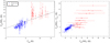 |
Fig. 8 Comparison of gas kinetic temperature derived from NH3 (2,2)/(1,1) ratios for Serpens South (blue points) and W 40 (red points) against dust temperature. The black line in the left panel indicates identical gas and dust temperature. |
4.3 Thermal and nonthermal motions
Previous observations of NH3 and H2CO in Galactic star-forming regions (e.g., Wouterloot et al. 1988; Molinari et al. 1996; Jijina et al. 1999; Wu et al. 2006; Urquhart et al. 2011, 2015; Wienen et al. 2012; Lu et al. 2014; Tang et al. 2017, 2018a,b) suggest that the line width is correlated with kinetic temperature. Our findings imply that the correlation between line width and kinetic temperature is due to the dissipation of turbulent energy.
Here we examine whether there is a relationship between turbulence and temperature in our survey area. We computed thermal velocity (vth), nonthermal velocity dispersion (σNT), and thermal sound speed (cs). vth, σNT, and cs are defined in Appendix A of Levshakov et al. (2014). For vth we have
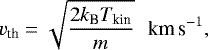 (6)
(6)
where kB is the Boltzmann constant, m is the mass of a particle, and Tkin is the kinetic temperature of the gas. For NH3, thermal velocity is
 (7)
(7)
The thermal contribution to the observed line with vobs is related to the above-mentioned FWHM line width by (see Appendix C)
 (8)
(8)
The vobs can be divided into a thermal and a turbulent part by
 (9)
(9)
where Δv is the FWHM line width of the NH3(1, 1) line obtained from the NH3(1, 1) fit in CLASS (see Sect. 2.2) and σNT is the nonthermal velocity dispersion along the line of sight:
 (10)
(10)
This value can be compared with the thermal sound speed,
 (11)
(11)
where μ = 2.37 is the mean molecular weight for molecular clouds (Dewangan et al. 2016) and mH is the mass of the hydrogen atom. Comparisons of velocity dispersion and kinetic temperature are shown in Fig. 9. The thermal velocity of NH3 (1,1) for lines detected at a >5σ level ranges from 0.09 to 0.18 km s−1 with an average of 0.11 ± 0.02 km s−1. The nonthermal velocity dispersion of NH3 (1,1) ranges from 0.07 to 0.55 km s−1 with an average of 0.34 ± 0.12 km s−1. The derived nonthermal motions of NH3 are much higher than the thermal line widths of our survey area, implying that the line broadening of NH3 is dominated by nonthermal motions in these clumps. The BGPS sources which contain both starless and active star forming massive cores observed by Dunham et al. (2011) show average thermal velocity and nonthermal velocity dispersions of 0.12 ± 0.02 and 0.76 ± 0.48 km s−1, respectively. Wienen et al. (2012) determined averages of 0.14 ± 0.02 and 0.90 ± 0.40 km s−1 for thermal velocity and nonthermal velocity dispersions, respectively in the cold high-mass clumps of the ATLASGAL survey. The average thermal velocity of our NH3 (1,1) data agrees with previous results observed in massive star-forming clumps (Dunham et al. 2011; Wienen et al. 2012), but our nonthermal velocity dispersions are smaller than their values.
We also calculated the thermal to nonthermal pressure ratio (RP =  /
/ ; Lada et al. 2003) and Mach number (given as M = σNT/cs). The sound speed ranges from 0.18 to 0.36 km s−1 with an average of 0.23 ± 0.04 km s−1. The thermal to nonthermal pressure ratio in the gas traced by NH3 (1,1) ranges from 0.16 to 6.07 with an average of 0.67 ± 0.79. The BGPS sources observed by Dunham et al. (2011) show that the RP values vary from 0.02 to 5.06 with an average of 0.20 ± 0.33. NH3 samples observed by Wienen et al. (2012) show values of 0.01–0.57 with an average of 0.10 ± 0.06. Our average value for thermal to nonthermal pressure ratio is higher than previous results observed byDunham et al. (2011) and Wienen et al. (2012). We find that the Mach number for NH3 (1,1) ranges from 0.41 to 2.47 with an average of 1.49 ± 0.45. The BGPS sources observed by Dunham et al. (2011) yield a mean Mach number of 3.2 ± 1.8. The average value of the Mach number we derive from NH3 may also be below the result (3.4 ± 1.1) of the various stages of high-mass star formation clumps with strong NH3 emission from the ATLASGAL survey (Wienen et al. 2012). Nevertheless, all this suggests that nonthermal pressure and supersonic nonthermal motions (e.g., turbulence, outflows, shocks, and/or magnetic fields) are dominant in the dense gas traced by NH3 in the Aquila region.
The derived values of vth, σNT, cs, RP, and Mach number for Serpens South and W 40 are listed separately in Table 2. We calculated average nonthermal line widths of NH3 (1,1) for those positions with NH3 (1,1) > 5σ features in the subsamples consisting of Serpens South and W 40. For NH3 (1,1), the average nonthermal line widths σNT are 0.32 ± 0.12 km s−1 and 0.41 ± 0.08 km s−1, respectively, that is, quite similar. The average nonthermal line widths of NH3 (1,1) calculated here are consistent with those found in Serpens South by Friesen et al. (2016). These latter authors suggested that much of the dense gas in Serpens South has subsonic or trans-sonic nonthermal motions, while the mean σNT across the region is similar to the expected ~0.2 km s−1 sound speed at 11 K.
The similar nonthermal line widths between the W 40 region and Serpens South are surprising. Either the entire region is already strongly affected by the consequences of massive star formation (e.g., through outflows and shocks) based on activity related to W 40 or the young low-mass stars in Serpens South are of sufficient number to induce turbulent motions to similar degree to that of the more massive stars in W 40, which may have dissociated or expelled most of the dense molecular gas in their vicinity. Figure 9 shows that turbulent heating considerably contributes to gas temperature in these clumps.
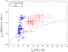 |
Fig. 9 Nonthermal velocity dispersion (σNT) vs. gas kinetic temperature derived from para-NH3 (1,1) for Serpens South (blue points) and W 40 (red points). The total dispersion of individual hyperfine structure (hfs) components are derived from the GILDAS built-in “NH3 (1, 1)” fitting method for the (1,1) line. The black lines represent the thermal sound speed. |
4.4 Radiative heating
Previous SCUBA-2 450 and 850 μm observationsof the W 40 complex in the Serpens-Aquila region (Rumble et al. 2016) provide evidence for radiative heating. The W 40 complex represents a HMSF region dominated by an OB association that is powering an H II region. OS1a is the most luminous star in the W 40 complex (Rumble et al. 2016), but heating by the associated nearby (D ≤ 0.1 pc) sources IRS1, IRS1a, IRS2, IRS2a, IRS2b, IRS3, and IRS3a (their positions are indicated in Fig. 6) is also likely playing a role.
We investigate the relationship between gas kinetic temperature and projected distance R from the central part of W 40 (OS1a, l = 28.79°, b = 3.49°) in Fig. 10. As is shown in the figure and as mentioned in Sect. 4.2, dust temperatures are lower than gas temperatures derived from NH3 in W 40.
It is expected that the gas temperature and distance relation from the Stefan-Boltzmann blackbody radiation law is Tkin = 100 ×
 K, adopting a molecular cloud distance of 436 pc (Ortiz-León et al. 2017, 2018) and assuming that OS1a is the dominant source with an approximate luminosity of 105.25 L⊙ (Kuhn et al. 2010; Wiseman & Ho 1998). For the emissivity of the dust grains smaller than the wavelength at the characteristic blackbody temperature, the radiation law is adjusted to Tkin = 100 ×
 K (Wiseman & Ho 1998).
The two radiation models for gas heating (Stefan-Boltzmann blackbody radiation and its modification related to dust emissivity) are both not well supported by our para-NH3 data (Fig. 10) which exclude positions related to Serpens South. Contrary to our expectation, temperatures near ~18′ (~2 pc) offsets appear to be slightly higher than those at ~5′ offsets. Thisholds for temperatures derived by both the gas and dust and is not in agreement with the declining dust temperatures found by Rumble et al. 2016 (their Fig. 15) as a function of distance from the main stellar source of W 40. For NH3 this may imply that the dense molecular gas in the vicinity of W 40 has been destroyed by UV radiation (Sect. 4.1) and that the projected angular distances in Fig. 10 may be significantly below the real distances. In any case, dust grain mantle evaporation as seen in hot cores (e.g., in Orion-KL) and leading to very high ammonia column densities is not seen. W 40 might have gone through such a phase of evolution, but UV photons may have destroyed its short-lived chemical consequences (for models, see e.g., Charnley et al. 1992) in the meantime. As discussed in Sect. 4.1, Serpens South shows a fractional total-NH3 abundance with an average of 8.6 (±3.8) × 10−8. In W 40, values are lower 1.6 (±1.4) × 10−8, which is a factor of ~5 below the result from Serpens South.
The nature of the molecular ridge, which is not particularly pronounced in the dust continuum maps of Fig. 1 but dominates the maps of NH3 emission in Figs. 3, 4, and 6, is still poorly defined. It could represent a PDR similar to the Orion bar northwest of the Trapezium stars (Tang et al. 2018a), or swept up material near the edge of an expanding H II region. Since radial velocities (see Fig. 4) do not hint at a significant difference between W 40 and Serpens South, such material would have been swept up mostly along the plane of the sky. Additional molecular surveys addressing the detailed chemistry of this region could shed more light on this puzzle.
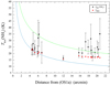 |
Fig. 10 Gas kinetic temperature derived from para-NH3 (black points) and dust temperature (red points) along the W 40 region (projected distance from its main stellar source OS1a, l = 28.79°, b = 3.49°). The blue and green lines are the expected relationships from a Stefan-Boltzmann law and modified Stefan-Boltzmann law (see Sect. 4.4), respectively, assuming OS1a is the dominant source with an approximate luminosity of 105.25 L⊙ (Kuhn et al. 2010; Rumble et al. 2016). |
4.5 Kinematics of the dense gas
To study the velocity pattern of our observed area in more detail, we fitted the velocities of the entire measured region, Serpens South, and W 40. There may be weak velocity gradients that run along the entire observed region, Serpens South, and W 40 (see left panel of Fig. 4). Following the steps of Goodman et al. (1993) and Wu et al. (2018), we fitted the velocity adopting a linear form: VLSR = v0 + a × Δl + b × Δb, where v0 is the systemic velocity of the cloud, and Δl and Δb are offsets in Galactic longitude and Galactic latitude. The velocity gradient can be derived as  , where distance D = 436 pc (Sect. 1). This distance was used for all spectra with peak line fluxes larger than 5σ. This linear velocities fitting is based on solid body approximations for Serpens South and W 40, Serpens South alone, and W 40 alone (see Table 1 for the adopted extent of those regions). The derived gradients are then 0.16 ± 0.01, 0.27 ± 0.01, and 0.38 ± 0.01 km s−1 pc−1 for the observed region shown in Fig. D.1, Serpens South, and W 40, respectively.
To check the assumption of solid body rotation we study the fitted velocity and velocity residuals (Vobs −Vfit) in Appendix D for the region encompassing both Serpens South and W 40. The black solid polyline indicates a potential rotation axis (0.019Δl + 0.007Δb − 0.328 = 0, in arcmin) in the fitted velocity map of the entire observed region (Fig. D.1 left panel), and three black parallel lines perpendicular to this rotation axis show the direction of the velocity gradient. Velocities tend to be lower in the lower right of the left panel of Fig.D.1. For Serpens South alone (see Table 1 for the extent of the region), the rotation axis is 0.03Δl − 0.01Δb − 0.12 = 0, and for W 40 it is 0.04Δl − 0.03Δb − 0.88 = 0 arcmin. From Fig. D.1, we can see that most of the velocity residuals are distributed in the range Vobs – Vfit = –1 to 1 km s−1 which is even more clearly shown in Fig. D.2. To be specific, 90% of the velocity residuals of the observed region shown in Fig. D.1, Serpens South, and W 40 are in the range Vobs−Vfit < 0.65, 0.56, and 0.79 km s−1, respectively.Larger velocity residuals are mainly located, in terms of Galactic coordinates, at the western and northeastern part of Serpens South and the southern part of W 40.
A maximum velocity gradient of 0.38 ± 0.01 km s−1 pc−1 for W 40 can be considered as an upper limit for an estimate of the rotational energy. Taking Serpens South and W 40 as a rigidly rotating cylinder, the ratio of rotational to gravitational energy is given (Bonnell et al. 1992; Wu et al. 2018) by
 (12)
(12)
where G is the gravitational constant and ρ, L, R, and ω are the density, height, radius, and the angular velocity of the cylinder. This can be simplified to
 (13)
(13)
where, ω−14 is the angular velocity in units of 10−14 s−1 and the gas density n4 is in units of104 cm−3 (Levshakov et al. 2013). For the entire observed region, Serpens South, and W 40, we adopt angular velocities, which are equal to the velocity gradients calculated before, 0.51, 0.88, and 1.23× 10⁻¹⁴ s−1 and an average density of the molecular Aquila complex of 104 cm−3 (Levshakov et al. 2013). From Eq. (13), the ratio of rotational to gravitational energy for the entire observed region, Serpens South, and W 40 we obtained are β ≲ 0.003, 0.01, and 0.02, respectively. It is clear that in the entire observed region, Serpens South, and W 40, rotation is presently playing a negligible role. The rotational energy is a very small fraction of the gravitational energy.
Using parallax measurements taken with the Very Large Baseline Array (VLBA), Ortiz-León et al. (2017, 2018) obtain distances slightly in excess of 400 pc for both Serpens South and the W 40 region, which together show an arc-like morphology (see Figs. 1, 3, B.1). However, including the weaker region 5 (Fig. 1) and the high and low Galactic latitude regions of region 4 (again Fig. 1), we encounter a ring-like morphology, possibly forming a shell of gas. One important question is whether or not the weakly emitting high-Galactic-longitude part of this ring is located at a similar distance to that obtained by Ortiz-León et al. (2017, 2018). While this remains an open question, we note that this high-longitude part of the putative shell shows about the same radial velocities as Serpens South and W 40 (Sect. 3.1). With respect to any Galactic kinematical model, clouds with similar radial velocity and not more than one degree apart should be located at similar distances.
While we cannot prove that similar kinematic distances correspond in our case to a physical connection, it is nevertheless worthwhile to analyze the observed structure with this assumption, noting that a similar morphology is also seen in 13 CO (which likely traces lower density gas than NH3) in Fig. 10 of Su et al. (2020) and in the H2 column density map of Könyves et al. (2010). The ring-like large-scale morphology of both the dust (Fig. 1) and the 13 CO- and NH3-emitting gas (Fig. 15 of Su et al. 2019 and our Figs. 3 and B.1) is reminiscent of an expanding interstellar bubble with large amounts of dense gas on one side and lesser amounts of such gas on the other.
Since velocities in regions 1 and 5 (see Fig. 1) are similar (Sect. 3.1), they might represent those parts of the putative shell that are expanding parallel to the plane of the sky. However this would mean that velocities inside the rim of this structure should be different, more redshifted on the back and more blueshifted on the front side. For all three rotation axes crossing the low-Galactic-longitude side of the shell-like structure, lower velocities and blueshifted areas are located at lower Galactic longitudes, while higher velocities and redshifted areas are located at higher longitudes. This is compatible with a radial motion of the entire shell-like structure and would indicate slow expansion, if the gas at higher longitudes forms a part of the back side of the shell, or slow contraction, if the gas is part of the front side of the shell. The velocity difference is about 0.7 km s−1.
For the kinematic age of the putative expanding shell, with
 (14)
(14)
rx and ry ~ 3.5 pc, and vexp = 0.7 km s−1 we obtain a timescale of several million years. However, we note that the 0.7 km s−1 are for this approach only a lower limit: (1) we do not see gas along the center of the putative shell, where the discrepancy in velocity relative to its rim should be largest; (2) the expansion of the gas may have significantly slowed down due to entrainment of ambient gas originally not participating in this expansion.
In this context it may be worth noting that the center of the putative shell is not known to host a supernova remnant (W. Reich, priv. comm.). More sensitive data, in particular from the high-Galactic-longitude parts of the ring-like structure (see Figs. 1 and 3) would be helpful to further investigate related scenarios.
5 Summary
We mapped the western part of the Aquila Rift cloud complex in the NH3 (1,1) and (2,2) transitions, which includes the densest regions of Serpens South and W 40. The main results of this work can be summarized as follows.
- 1.
The NH3 morphology, revealing the distribution of the dense gas (n(H2) ≳ 10−3 cm−3), is correlated with that of the Herschel infrared dust emission and shows an overall similar structure with two exceptions: there is, in Galactic coordinates, the well-known NE–SW ridge of dense gas, which forms the core of the Serpens South region and is much more dominant in NH3 than in the dust emission. W 40 dominates the dust emission but is much less pronounced in NH3. The ridge with strong NH3 (1,1) emission contains several cores along a total length of about 15′. Weaker emission extends further to lower and higher Galactic latitudes and toward regions at larger longitudes. Overall, the NH3 distribution forms, like the dust, a circle with a diameter of 50′–60′ (~7 pc), with comparatively strong emission at low and weak emission at high longitudes.
- 2.
The kinetic temperature of the dense gas in the Aquila rift cloud complex measured by NH3 (2,2)/(1,1) line ratios ranges from 8.9 to 35.0 K with an average of 15.3 ± 6.1 K. The HMSF region of W 40 has a gas kinetic temperature of ~25 K, which is twice that (~12 K) found in the LMSF region of Serpens South.
- 3.
Fractional abundances of total NH3 vary from 0.1 ×10⁻⁸ to 2.1 ×10⁻⁷ with an average of 6.9 (±4.5) × 10−8. Serpens South has total NH3 fractional abundances also ranging from 0.2 ×10⁻⁸ to 2.1 ×10⁻⁷ with an average of 8.6 (±3.8) × 10−8. Lower values of 0.1 – 4.3 ×10⁻⁸ with an average of 1.6 (±1.4) × 10−8 characterize W 40, which is a factor of approximately five below the result from Serpens South.
- 4.
A comparison of kinetic temperatures derived from NH3 and dust emission indicates that gas and dust temperatures are in agreement in Serpens South, but gas temperatures are higher than those of the dust in W 40. This suggests that gas and dust are coupled in Serpens South, but not in W 40.
- 5.
Dense gas traced by NH3 is significantly influenced by supersonic nonthermal motions. Similar levels of nonthermal turbulence are encountered in W 40 and Serpens South. This may either be caused by the fact that the entire region is already strongly affected by the consequences of massive star formation based on activity related to W 40 or that a similar amount of turbulence is triggered by the large number of forming low-mass stars in Serpens South. W 40 appears to have dissociated or expelled most dense molecular gas in its vicinity.
- 6.
The nonthermal velocity dispersion of NH3 (1,1) is positively correlated with the gas temperature, which indicates that the dense gas may be heated by dissipation of turbulent energy.
- 7.
Velocity gradients of 0.16 ± 0.01, 0.27 ± 0.01, and 0.38 ± 0.01 km s−1 pc−1 appear to be present in the observed region shown in Fig. D.1, Serpens South alone, and W 40 alone, respectively. The rotational and gravitational energy of the Aquila region are compared using those velocity gradients. For the entire observed region, Serpens South, and W 40, ratios are about β ≲ 0.003, 0.01, and 0.02, respectively. This demonstrates that the rotational energy is a negligible fraction of the gravitational energy.
- 8.
The morphology of the entire studied region can be described by a ring or shell with a diameter of about 7 pc and strong emission at lower Galactic longitudes and weak emission at higher Galactic longitudes. However, this only holds in a physical sense, if all parts are located at approximately the same distance. This is presently only known for the lower-Galactic-longitude part with its strong emission. While we find velocity gradients in the radial direction at the low-longitude side of the putative shell, it is therefore not yet clear whether this indicates a systematic expansion (or contraction) of the entire structure.
Acknowledgements
We would like to thank the anonymous referee for the useful suggestions that improved this study. The authors are thankful for helpful comments by Wolfgang Reich. We thank the staff of the Nanshan 26-m radio telescope for their assistance during the observations. This work is based on measurements made with the Nanshan 26-m radio telescope, which is operated by the Key Laboratory of Radio Astronomy, Chinese Academy of Sciences. This work was funded by the National Natural Science foundation of China under grant 11433008, 11903070, 11603063, 11703074, 11703073, and 11973076, the Heaven Lake Hundred-Talent Program of Xinjiang Uygur Autonomous Region of China, and the CAS “Light of West China” Program under Grant 2018-XBQNXZ-B-024, 2016-QNXZ-B-23, and 2016-QNXZ-B-22. C.H. acknowledges support by a Chinese Academy of Sciences President’s International Fellowship Initiative for visiting scientists (2021VMA0009). This research has used NASA’s Astrophysical Data System (ADS).
Appendix A Calibration stability
The system temperature was calibrated against a signal injected by a noise diode. Hot (ambient temperature) and cold (liquid nitrogen) loads determine the temperature of the noise diode. We observed the reference position (RA: 00:36:47.51, Dec: +63:29:02.1 with (0,0) offset, J2000) to check the calibration stability every 2–3 h. All reference position observations were made in the OTF mode of a small area of 6′ × 6′. To present the peak distribution against elevation (Fig. A.1), we regridded the data and then fitted the NH3 (1,1) main lines (the central group of NH3 (1,1) hyperfine components). From Fig. A.1, we clearly see that there is no significant systematic variation. The standard deviations of the mean of the peak intensities is about 10%, thus the observational system of the Nanshan observatory is stable.
To further check our calibration stability, the NH3 (1,1) data of G035.39-0.33 collected using the GBT (Sokolov et al. 2017) were used as a comparision with our NH3 data. For the process, the GBT data were smoothed to our beam size using the “XY_MAP” routine in GILDAS. In Fig. A.2, the GBT spectrum (black) and our spectrum (red) of the reference position (RA: 18:57:07.94, Dec: 02:10:51.40, J2000) are displayed. The two spectra can clearly be seen to match each other well and the checking results are reliable.
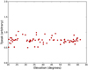 |
Fig. A.1 Uncorrected NH3 (1,1) main line intensities against elevation of repeated observations toward the reference position. The position corresponds to RA: 00:36:47.51, Dec: +63:29:02.1 (J2000). The standard deviations of the mean of the flux is about 10%. |
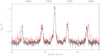 |
Fig. A.2 NH3 (1,1) spectra from the GBT (black) and our data (red) toward the reference position RA: 18:57:07.94, Dec: 02:10:51.40 (J2000). |
Appendix B Prestellar and protostellar cores and NH3 spectra toward the Aquila Rift cloud complex and derived physical parameters
In this appendix we present prestellar and protostellar cores taken from Könyves et al. (2015) (see Fig. B.1), and show the NH3 spectra for the 38 Clumps identified with Clumpfind2d in Sect. 3.2. The observed spectra of the NH3 (1,1) and (2,2) transitions detected toward their peak positions are shown in Figs. B.2 and B.3. Measured physical parameters are listed in Tables B.1–B.3.
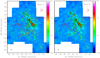 |
Fig. B.1 Integrated intensity maps of NH3 (1,1) (left and right). The reference position is l = 28.59°, b = 3.55°. The integration range is 4 < VLSR < 10 km s−1. Contours start at 0.13 K km s−1 (3σ) on a main beam brightness temperature scale and go up in steps of 0.13 K km s−1. The unit of the color bars is K km s−1. The half-power beam width is illustrated as a black filled circle in the lower left corners of the images. Left and right panels: the red points show the positions of the 362 candidate prestellar cores and 49 protostellar cores taken from Könyves et al. (2015), respectively. The red line in the top right of each map illustrates the 1 pc scale at a distance of 436 pc (Ortiz-León et al. 2017, 2018). |
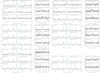 |
Fig. B.2 NH3 (1,1) and (2,2) spectra towards clumps 01 to 17. Green colour indicates the NH3 (1,1) fitting and Gaussian fitting of the NH3 (2,2) lines (see Sect. 2.2). The central position of this area is at (l, b) = (28.59°, 3.55°). Offsets in Galactic coordinates (unit: arcmin) are shown in the top right corner of each NH3 (1,1) panel. |
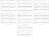 |
Fig. B.3 NH3 (1,1) spectra towards clumps 18 to 38. Green color indicates the NH3 (1,1) fitting of the NH3 (1,1) lines. The central position of this area is at (l, b) = (28.59°, 3.55°). Offsets in Galactic coordinates (unit: arcmin) are shown in the top right corner of each NH3 (1,1) panel. |
Calculated model parameter of NH3 (1,1) and NH3 (2,2) emission lines detected in 17 clumps.
Appendix C Uncertainty estimation and derivation of the physical parameters
The uncertainty of Trot in Eq. (1) is
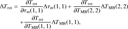 (C.1)
(C.1)
where Δτm(1, 1), ΔTMB(2, 2) and ΔTMB(1, 1) are uncertainties of τm(1, 1), TMB(2, 2) and TMB(1, 1), respectively.
The error of Tkin in Eq. (2) is
 (C.2)
(C.2)
Uncertainties of Ntot in Eq. (3) are
 (C.3)
(C.3)
where ΔN(1, 1) is the uncertainty of N(1, 1) in Eq. (4).
When τ ≪ 1, N(1, 1) is given by

The uncertainty of N(1,1) then becomes

where ΔΔv represents the error in the line width Δv. If τ ≳ 1, Tex is obtained from Eq. (5) as a function of TMB and τ, then the uncertainty of N(1, 1) is defined by
 (C.8)
(C.8)
Conversion of measured FWHM line widths into velocity dispersion: the intensity of a line with Gaussian distribution at radial velocity vr is
 (C.9)
(C.9)
where vp is the peak velocity, and σ is the velocity dispersion. From the definition of the FWHM, we can infer
 (C.10)
where Δv is the FWHM.
Conversion of velocity dispersion into thermal contribution to the observed line width (see Eq.(8)):
 (C.11)
Appendix D Fitted velocity and residuals of the velocity fitting
We have assumed that the observed region shown in Fig. D.1 is a rigid body and fitted its velocity field in a linear form. To check this assumption, we present the distribution of the fitted velocity (Fig. D.1 left panel) and velocity residuals (Fig. D.1 right panel) between the observed velocity and the fitted velocity. Statistics of the velocity residuals are shown in Fig. D.2. From the right panel of Fig. D.1, we can see that most of our velocity residuals are in the range of Vobs–Vfit = –1 to 1 km s−1, which can be even more clearly seen in Fig. D.2. Specifically, 90% of the velocity residuals of the shown region, Serpens South alone, and W 40 alone are in the range Vobs−Vfit < 0.65, 0.56, and 0.79 km s−1, respectively. Larger velocity residuals are mainly located, in Galactic coordinates, at the western and northeastern part of the Serpens South and the southern part of the W 40.
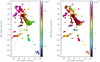 |
Fig. D.1 Fitted velocity (left) and velocity residual (Vobs – Vfit) (right) maps of the NH3 (1,1) lines with S∕Ns >5σ. Contours are as in Figs. 4 and 6. The black solid polyline in the left panel indicates a potential rotation axis, and three black parallel lines perpendicular to the rotation axis show the direction of the velocity gradient. |
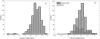 |
Fig. D.2 Histograms of the velocity residuals (Vobs – Vfit) derived fromour NH3 (1,1) data with S∕Ns >5σ: (a) entire observed region, (b) Serpens South and W 40. |
References
- André, P., Men’shchikov, A., Bontemps, S., et al. 2010, A&A, 518, L102 [NASA ADS] [CrossRef] [EDP Sciences] [Google Scholar]
- Barranco, J. A., & Goodman, A. A. 1998, ApJ, 504, 207 [NASA ADS] [CrossRef] [Google Scholar]
- Batrla, W., & Wilson, T. L. 2003, A&A, 408, 231 [NASA ADS] [CrossRef] [EDP Sciences] [Google Scholar]
- Battersby, C., Bally, J., Dunham, M., et al. 2014, ApJ, 786, 116 [NASA ADS] [CrossRef] [Google Scholar]
- Benson, P. J., & Myers, P. C. 1983, ApJ, 270, 589 [NASA ADS] [CrossRef] [Google Scholar]
- Bonnell, I., Arcoragi, J.-P., Martel, H., et al. 1992, ApJ, 400, 579 [NASA ADS] [CrossRef] [Google Scholar]
- Bontemps, S., André, P., Könyves, V., et al. 2010, A&A, 518, L85 [NASA ADS] [CrossRef] [EDP Sciences] [Google Scholar]
- Charnley, S. B., Tielens, A. G. G. M., & Millar, T. J. 1992, ApJ, 399, L71 [NASA ADS] [CrossRef] [Google Scholar]
- Cheung, A. C., Rank, D. M., Townes, C. H., et al. 1969, ApJ, 157, L13 [NASA ADS] [CrossRef] [Google Scholar]
- Chira, R.-A., Beuther, H., Linz, H., et al. 2013, A&A, 552, A40 [NASA ADS] [CrossRef] [EDP Sciences] [Google Scholar]
- Danby, G., Flower, D. R., Valiron, P., et al. 1988, MNRAS, 235, 229 [NASA ADS] [CrossRef] [Google Scholar]
- Dewangan, L. K., Ojha, D. K., Luna, A., et al. 2016, ApJ, 819, 66 [NASA ADS] [CrossRef] [Google Scholar]
- Dunham, M. K., Rosolowsky, E., Evans, N. J., II, et al. 2010, ApJ, 717, 1157 [NASA ADS] [CrossRef] [Google Scholar]
- Dunham, M. K., Rosolowsky, E., Evans, N. J., II, et al. 2011, ApJ, 741, 110 [NASA ADS] [CrossRef] [Google Scholar]
- Dobashi, K., Uehara, H., Kandori, R., et al. 2005, PASJ, 57, S1 [NASA ADS] [CrossRef] [Google Scholar]
- Evans, N. J., II 1999, ARA&A, 37, 311 [NASA ADS] [CrossRef] [Google Scholar]
- Faure, A., Hily-Blant, P., Le Gal, R., et al. 2013, ApJ, 770, L2 [NASA ADS] [CrossRef] [Google Scholar]
- Foster, J. B., Rosolowsky, E. W., Kauffmann, J., et al. 2009, ApJ, 696, 298 [NASA ADS] [CrossRef] [Google Scholar]
- Friesen, R. K., Bourke, T. L., Di Francesco, J., Gutermuth, R., Myers, P. C. 2016, ApJ, 833, 204 [NASA ADS] [CrossRef] [Google Scholar]
- Friesen, R. K., Pineda, J. E., co-PIs, et al. 2017, ApJ, 843, 63 [NASA ADS] [CrossRef] [Google Scholar]
- Giannetti, A., Brand, J., Sánchez-Monge, Á., et al. 2013, A&A, 556, A16 [NASA ADS] [CrossRef] [EDP Sciences] [Google Scholar]
- Goodman, A. A., Benson, P. J., Fuller, G. A., et al. 1993, ApJ, 406, 528 [NASA ADS] [CrossRef] [Google Scholar]
- Goldsmith, P. F. 2001, ApJ, 557, 736 [NASA ADS] [CrossRef] [MathSciNet] [Google Scholar]
- Gutermuth, R. A., Bourke, T. L., Allen, L. E., et al. 2008, ApJ, 673, L151 [NASA ADS] [CrossRef] [Google Scholar]
- Ho, P. T. P., & Townes, C. H. 1983, ARA&A, 21, 239 [NASA ADS] [CrossRef] [Google Scholar]
- Hunter, J. D. 2007, Comput. Sci. Eng., 9, 90 [NASA ADS] [CrossRef] [Google Scholar]
- Jijina, J., Myers, P. C., & Adams, F. C. 1999, ApJS, 125, 161 [NASA ADS] [CrossRef] [Google Scholar]
- Komesh, T., Esimbek, J., Baan, W., et al. 2019, ApJ, 874, 172 [CrossRef] [Google Scholar]
- Könyves, V., André, P., Men’shchikov, A., et al. 2010, A&A, 518, L106 [NASA ADS] [CrossRef] [EDP Sciences] [Google Scholar]
- Könyves, V., André, P., Men’shchikov, A., et al. 2015, A&A, 584, A91 [NASA ADS] [CrossRef] [EDP Sciences] [Google Scholar]
- Koumpia, E., Harvey, P. M., Ossenkopf, V., et al. 2015, A&A, 580, A68 [NASA ADS] [CrossRef] [EDP Sciences] [Google Scholar]
- Kuhn, M. A., Getman, K. V., Feigelson, E. D., et al. 2010, ApJ, 725, 2485 [NASA ADS] [CrossRef] [Google Scholar]
- Lada, C. J., & Lada, E. A. 2003, ARA&A, 41, 57 [NASA ADS] [CrossRef] [Google Scholar]
- Lada, C. J., Bergin, E. A., Alves, J. F., & Huard, T. L. 2003, ApJ, 586, 286 [NASA ADS] [CrossRef] [Google Scholar]
- Larsson, B., Liseau, R., Bergman, P., et al. 2003, A&A, 402, L69 [NASA ADS] [CrossRef] [EDP Sciences] [Google Scholar]
- Levshakov, S. A., Henkel, C., Reimers, D., et al. 2013, A&A, 553, A58 [NASA ADS] [CrossRef] [EDP Sciences] [Google Scholar]
- Levshakov, S. A., Henkel, C., Reimers, D., & Wang, M. 2014, A&A, 567, A78 [NASA ADS] [CrossRef] [EDP Sciences] [Google Scholar]
- Lu, X., Zhang, Q., Liu, H. B., Wang, J., & Gu, Q. 2014, ApJ, 790, 84 [NASA ADS] [CrossRef] [Google Scholar]
- Mallick, K. K., Kumar, M. S. N., Ojha, D. K., et al. 2013, ApJ, 779, 113 [NASA ADS] [CrossRef] [Google Scholar]
- Mauersberger, R., Henkel, C., Wilson, T. L., & Walmsley, C. M. 1986, A&A, 162, 199 [Google Scholar]
- Mauersberger, R., Henkel, C., & Wilson, T. L. 1987, A&A, 173, 352 [NASA ADS] [Google Scholar]
- Merello, M., Molinari, S., Rygl, K. L. J., et al. 2019, MNRAS, 483, 5355 [NASA ADS] [CrossRef] [Google Scholar]
- Molinari, S., Brand, J., Cesaroni, R., & Palla, F. 1996, A&A, 308, 573 [NASA ADS] [Google Scholar]
- Myers, P. C., & Benson, P. J. 1983, ApJ, 266, 309 [NASA ADS] [CrossRef] [Google Scholar]
- Myers, P. C., Dame, T. M., Thaddeus, P., et al. 1986, ApJ, 301, 398 [NASA ADS] [CrossRef] [Google Scholar]
- Nakamura, F., Dobashi, K., Shimoikura, T., Tanaka, T., & Onishi, T. 2017, ApJ, 837, 154 [NASA ADS] [CrossRef] [Google Scholar]
- Ortiz-León, G. N., Dzib, S. A., Kounkel, M. A., et al. 2017, ApJ, 834, 143 [NASA ADS] [CrossRef] [Google Scholar]
- Ortiz-León, G. N., Loinard, L., Dzib, S. A., et al. 2018, ApJ, 869, L33 [NASA ADS] [CrossRef] [Google Scholar]
- Ott, J., Henkel, C., Staveley-Smith, L., et al. 2010, ApJ, 710, 105 [NASA ADS] [CrossRef] [Google Scholar]
- Pandian, J. D., Wyrowski, F., & Menten, K. M. 2012, ApJ, 753, 50 [NASA ADS] [CrossRef] [Google Scholar]
- Persson, C. M., De Luca, M., Mookerjea, B., et al. 2012, A&A, 543, A145 [NASA ADS] [CrossRef] [EDP Sciences] [Google Scholar]
- Rodríguez, L. F., Rodney, S. A., & Reipurth, B. 2010, AJ, 140, 968 [CrossRef] [Google Scholar]
- Rohlfs, K., & Wilson, T. L. 2004, Tools of Radio Astronomy, eds. K. Rohlfs, & T. L. Wilson (Berlin: Springer), 2004 [Google Scholar]
- Rumble, D., Hatchell, J., Pattle, K., et al. 2016, MNRAS, 460, 4150 [NASA ADS] [CrossRef] [Google Scholar]
- Schreyer, K., Henning, T., Koempe, C., & Harjunpaeae, P. 1996, A&A, 306, 267 [Google Scholar]
- Shirley, Y. L. 2015, PASP, 127, 299 [NASA ADS] [CrossRef] [Google Scholar]
- Smith, J., Bentley, A., Castelaz, M., et al. 1985, ApJ, 291, 571 [NASA ADS] [CrossRef] [Google Scholar]
- Sokolov, V., Wang, K., Pineda, J. E., et al. 2017, A&A, 606, A133 [NASA ADS] [CrossRef] [EDP Sciences] [Google Scholar]
- Su, Y., Yang, J., Zhang, S., et al. 2019, ApJS, 240, 9 [NASA ADS] [CrossRef] [Google Scholar]
- Su, Y., Yang, J., Yan, Q.-Z., et al. 2020, ApJ, 893, 91 [CrossRef] [Google Scholar]
- Suzuki, H., Yamamoto, S., Ohishi, M., et al. 1992, ApJ, 392, 551 [NASA ADS] [CrossRef] [Google Scholar]
- Tafalla, M., Myers, P. C., Caselli, P., & Walmsley, C. M. 2004, A&A, 416, 191 [NASA ADS] [CrossRef] [EDP Sciences] [Google Scholar]
- Tafalla, M., Santiago-García, J., Myers, P. C., et al. 2006, A&A, 455, 577 [NASA ADS] [CrossRef] [EDP Sciences] [Google Scholar]
- Takano, S., Nakai, N., & Kawaguchi, K. 2002, PASJ, 54, 195 [NASA ADS] [CrossRef] [Google Scholar]
- Tan, J. C., Beltrán, M. T., Caselli, P., et al. 2014, Protostars and Planets VI (Tucson, AZ: University of Arizona Press), 149 [Google Scholar]
- Tang, X.D., Henkel, C., Menten, K. M., et al. 2017, A&A, 598, A30 [NASA ADS] [CrossRef] [EDP Sciences] [Google Scholar]
- Tang, X. D., Henkel, C., Menten, K. M., et al. 2018a, A&A, 609, A16 [NASA ADS] [CrossRef] [EDP Sciences] [Google Scholar]
- Tang, X. D., Henkel, C., Wyrowski, F., et al. 2018b, A&A, 611, A6 [NASA ADS] [CrossRef] [EDP Sciences] [Google Scholar]
- Ungerechts, H., Walmsley, C. M., & Winnewisser, G. 1986, A&A, 157, 207 [Google Scholar]
- Urquhart, J. S., Morgan, L. K., Figura, C. C., et al. 2011, MNRAS, 418, 1689 [NASA ADS] [CrossRef] [Google Scholar]
- Urquhart, J. S., Figura, C. C., Moore, T. J. T., et al. 2015, MNRAS, 452, 4029 [NASA ADS] [CrossRef] [Google Scholar]
- Vallee, J. P. 1987, A&A, 178, 237 [NASA ADS] [Google Scholar]
- Walmsley, C. M., & Ungerechts, H. 1983, A&A, 122, 164 [Google Scholar]
- Weiß, A., Neininger, N., Henkel, C., Stutzki, J., & Klein, U. 2001, ApJ, 554, L143 [NASA ADS] [CrossRef] [Google Scholar]
- Wienen, M., Wyrowski, F., Schuller, F., et al. 2012, A&A, 544, A146 [NASA ADS] [CrossRef] [EDP Sciences] [Google Scholar]
- Williams, J. P., de Geus, E. J., & Blitz, L. 1994, ApJ, 428, 693 [NASA ADS] [CrossRef] [Google Scholar]
- Wiseman, J. J., & Ho, P. T. P. 1998, ApJ, 502, 676 [NASA ADS] [CrossRef] [Google Scholar]
- Wouterloot, J. G. A., Walmsley, C. M., & Henkel, C. 1988, A&A, 203, 367 [NASA ADS] [Google Scholar]
- Wu, Y., Zhang, Q., Yu, W., et al. 2006, A&A, 450, 607 [NASA ADS] [CrossRef] [EDP Sciences] [Google Scholar]
- Wu, G., Qiu, K., Esimbek, J., et al. 2018, A&A, 616, A111 [CrossRef] [EDP Sciences] [Google Scholar]
- Young, K. E., Lee, J.-E., Evans, N. J., II, et al. 2004, ApJ, 614, 252 [NASA ADS] [CrossRef] [Google Scholar]
- Zeilik, M., II, & Lada, C. J. 1978, ApJ, 222, 896 [NASA ADS] [CrossRef] [Google Scholar]
- Zinnecker, H., & Yorke, H. W. 2007, ARA&A, 45, 481 [NASA ADS] [CrossRef] [Google Scholar]
All Tables
Calculated model parameter of NH3 (1,1) and NH3 (2,2) emission lines detected in 17 clumps.
All Figures
|
Fig. 1 Color image of the Aquila Rift (red for 500 μm, green for 350 μm, and blue for 250 μm, all derived from Herschel data; Bontemps et al. 2010; Könyves et al. 2010). The regions subsequently observed in NH3 are marked by six boxes (see Table A.1). |
| In the text | |
|
Fig. 2 NH3 (1,1) and (2,2) spectra at offset (Δl, Δb) = (2′, 16′) with respect to the reference position (l = 28.59°, b = 3.55°). In each panel, the black solid line represents the observed spectrum, the green solid line indicates the NH3 (1,1) fitting (lower panel) and Gaussian fitting (upper panel) of the NH3 (2,2) line (see Sect. 2.2). The groups of hyperfine components “mg”, “isg”, and “osg” represent the main, inner-satellite, and outer-satellite groups. The velocity scale is Local Standard of Rest, here and elsewhere. |
| In the text | |
|
Fig. 3 Integrated intensity maps of NH3 (1,1) (left) and (2,2) (right). The reference position is l = 28.59°, b = 3.55°. The integration range is 4 < VLSR < 10 km s−1. Contours start at 0.13 K km s−1 (3σ) on a main beam brightness temperature scale and go up in steps of 0.13 K km s−1. The unit of the color bars is K km s−1. The half-power beam width is illustrated as a black filled circle in the lower left corners of the images. The red line in the top right of each map illustrates the 1 pc scale at a distance of 436 pc (Ortiz-León et al. 2017, 2018). Left panel: black stars show the positions of the identified 38 ammonia clumps (see Sect. 3.2). |
| In the text | |
|
Fig. 4 Para-NH3 (1,1) intensity-weighted mean velocity (moment 1, left) and FWHM line width (moment 2, right) maps. The reference position is l = 28.59°, b = 3.55°. These intensity-weighted mean velocities and FWHM line widths referring to the individual hf components are derived from the GILDAS built-in “NH3 (1,1)” fitting method (Sect. 2.2). The considered velocity range is 4 < VLSR < 10 km s−1 for each panel. Contours of integrated intensity start at 0.23 K km s−1 (5σ) on a main beam brightness temperature scale and go up in steps of 0.23 K km s−1. |
| In the text | |
|
Fig. 5 Histograms of physical parameters derived from NH3. (a) Intrinsic FWHM line widths of individual NH3 (1,1) hyperfine structure components with a peak line flux threshold of 5σ; (b) peak optical depths of the main group of hf components τm(1, 1) for those positions with NH3 (1,1) S∕Ns > 5σ (these line widths and peak optical depths are derived from the GILDAS built-in “NH3 (1,1)” fitting method); (c) rotational temperature Trot, where both the NH3 (1,1) and (2,2) lines were detected, at levels of at least 5σ; (d) kinetic temperature Tkin, for those positions with NH3 (2,2) line detections and >5σ features; (e) para and total (para+ortho) column densities of NH3, for those positions exhibiting NH3 (2,2) line detections and >5σ features, assuming an ortho- to para-ratio in thermal equilibrium at the presently obtained kinetic temperature; (f) para-NH3 fractional abundance χ = [para-NH3]/[H2], and total-NH3 (para+ortho) fractional abundance χ = [total-NH3]/[H2], toward the positions with NH3 (2,2) line detections and >5σ features, again adopting ortho- to para NH3 ratios assuming thermal equilibrium. |
| In the text | |
|
Fig. 6 Maps of NH3 kinetic temperature in units of Kelvin (left), the logarithm of the total-NH3 column density in units of cm−2 (middle), and the corresponding logarithm of the fractional abundance (right). The reference position is l = 28.59°, b = 3.55°. Contours of integrated NH3 (1,1) intensity are the same as in Fig. 4 and cover the velocity range 4 < VLSR < 10 km s−1. Contours start at 0.23 K km s−1 (5σ) on a main beam brightness temperature scale and go up in steps of 0.23 K km s−1. Magenta stars show the locations of the OB association (OS1a, IRS1, IRS1a, IRS2, IRS2a, IRS2b, IRS3, and IRS3a) in W 40. |
| In the text | |
|
Fig. 7 Column densities derived from total-N(NH3) for Serpens South (blue points) and W 40 (red points) vs. N(H2) column densities (left), total column densities of N(NH3) vs. kinetic temperature (middle), and total fractional NH3 abundance, N(total-NH3)/N(H2), vs. kinetic temperature Tkin(NH3) (right). |
| In the text | |
|
Fig. 8 Comparison of gas kinetic temperature derived from NH3 (2,2)/(1,1) ratios for Serpens South (blue points) and W 40 (red points) against dust temperature. The black line in the left panel indicates identical gas and dust temperature. |
| In the text | |
|
Fig. 9 Nonthermal velocity dispersion (σNT) vs. gas kinetic temperature derived from para-NH3 (1,1) for Serpens South (blue points) and W 40 (red points). The total dispersion of individual hyperfine structure (hfs) components are derived from the GILDAS built-in “NH3 (1, 1)” fitting method for the (1,1) line. The black lines represent the thermal sound speed. |
| In the text | |
|
Fig. 10 Gas kinetic temperature derived from para-NH3 (black points) and dust temperature (red points) along the W 40 region (projected distance from its main stellar source OS1a, l = 28.79°, b = 3.49°). The blue and green lines are the expected relationships from a Stefan-Boltzmann law and modified Stefan-Boltzmann law (see Sect. 4.4), respectively, assuming OS1a is the dominant source with an approximate luminosity of 105.25 L⊙ (Kuhn et al. 2010; Rumble et al. 2016). |
| In the text | |
|
Fig. A.1 Uncorrected NH3 (1,1) main line intensities against elevation of repeated observations toward the reference position. The position corresponds to RA: 00:36:47.51, Dec: +63:29:02.1 (J2000). The standard deviations of the mean of the flux is about 10%. |
| In the text | |
|
Fig. A.2 NH3 (1,1) spectra from the GBT (black) and our data (red) toward the reference position RA: 18:57:07.94, Dec: 02:10:51.40 (J2000). |
| In the text | |
|
Fig. B.1 Integrated intensity maps of NH3 (1,1) (left and right). The reference position is l = 28.59°, b = 3.55°. The integration range is 4 < VLSR < 10 km s−1. Contours start at 0.13 K km s−1 (3σ) on a main beam brightness temperature scale and go up in steps of 0.13 K km s−1. The unit of the color bars is K km s−1. The half-power beam width is illustrated as a black filled circle in the lower left corners of the images. Left and right panels: the red points show the positions of the 362 candidate prestellar cores and 49 protostellar cores taken from Könyves et al. (2015), respectively. The red line in the top right of each map illustrates the 1 pc scale at a distance of 436 pc (Ortiz-León et al. 2017, 2018). |
| In the text | |
|
Fig. B.2 NH3 (1,1) and (2,2) spectra towards clumps 01 to 17. Green colour indicates the NH3 (1,1) fitting and Gaussian fitting of the NH3 (2,2) lines (see Sect. 2.2). The central position of this area is at (l, b) = (28.59°, 3.55°). Offsets in Galactic coordinates (unit: arcmin) are shown in the top right corner of each NH3 (1,1) panel. |
| In the text | |
|
Fig. B.3 NH3 (1,1) spectra towards clumps 18 to 38. Green color indicates the NH3 (1,1) fitting of the NH3 (1,1) lines. The central position of this area is at (l, b) = (28.59°, 3.55°). Offsets in Galactic coordinates (unit: arcmin) are shown in the top right corner of each NH3 (1,1) panel. |
| In the text | |
|
Fig. D.1 Fitted velocity (left) and velocity residual (Vobs – Vfit) (right) maps of the NH3 (1,1) lines with S∕Ns >5σ. Contours are as in Figs. 4 and 6. The black solid polyline in the left panel indicates a potential rotation axis, and three black parallel lines perpendicular to the rotation axis show the direction of the velocity gradient. |
| In the text | |
|
Fig. D.2 Histograms of the velocity residuals (Vobs – Vfit) derived fromour NH3 (1,1) data with S∕Ns >5σ: (a) entire observed region, (b) Serpens South and W 40. |
| In the text | |
Current usage metrics show cumulative count of Article Views (full-text article views including HTML views, PDF and ePub downloads, according to the available data) and Abstracts Views on Vision4Press platform.
Data correspond to usage on the plateform after 2015. The current usage metrics is available 48-96 hours after online publication and is updated daily on week days.
Initial download of the metrics may take a while.