| Issue |
A&A
Volume 642, October 2020
|
|
|---|---|---|
| Article Number | A44 | |
| Number of page(s) | 14 | |
| Section | The Sun and the Heliosphere | |
| DOI | https://doi.org/10.1051/0004-6361/202038668 | |
| Published online | 02 October 2020 | |
Sunspot penumbral filaments intruding into a light bridge and the resultant reconnection jets⋆
1
CAS Key Laboratory of Solar Activity, National Astronomical Observatories, Chinese Academy of Sciences, Beijing 100101, PR China
e-mail: This email address is being protected from spambots. You need JavaScript enabled to view it.
, This email address is being protected from spambots. You need JavaScript enabled to view it.
2
School of Astronomy and Space Science, University of Chinese Academy of Sciences, Beijing 100049, PR China
3
School of Physics and Materials Science, Anhui University, Hefei 230601, PR China
4
Yunnan Observatories, Chinese Academy of Sciences, Kunming 650011, PR China
Received:
16
June
2020
Accepted:
29
July
2020
Abstract
Context. Penumbral filaments and light bridges are prominent structures inside sunspots and are important for understanding the nature of sunspot magnetic fields and magneto-convection underneath.
Aims. We investigate an interesting event where several penumbral filaments intrude into a sunspot light bridge. In doing so we aim to gain further insight into the magnetic fields of the sunspot penumbral filament and light bridge, as well as their interaction.
Methods. Combining data from the New Vacuum Solar Telescope, Solar Dynamics Observatory, and Interface Region Imaging Spectrograph, we study the emission, kinematic, and magnetic topology characteristics of the penumbral filaments intruding into the light bridge and the resultant jets.
Results. At the west part of the light bridge, the intruding penumbral filaments penetrate into the umbrae on both sides of the light bridge, and two groups of jets are also detected. The jets share the same projected morphology with the intruding filaments and are accompanied by intermittent footpoint brightenings. Simultaneous spectral imaging observations provide convincing evidence for the presences of magnetic-reconnection-related heating and bidirectional flows near the jet bases and contribute to measuring the vector velocities of the jets. Additionally, nonlinear force-free field extrapolation results reveal strong and highly inclined magnetic fields along the intruding penumbral filaments, highly consistent with the results deduced from the vector velocities of the jets. Therefore, we propose that the jets could be caused by magnetic reconnections between emerging fields within the light bridge and the nearly horizontal fields of intruding filaments. The jets are then ejected outward along the stronger filament fields.
Conclusions. Our study indicates that magnetic reconnection could occur between the penumbral filament fields and emerging fields within the light bridge and produce jets along the stronger filament fields. These results further complement the study of magnetic reconnection and dynamic activities within the sunspot.
Key words: magnetic reconnection / Sun: activity / Sun: atmosphere / Sun: magnetic fields / sunspots
Movies associated to Figs. 1, 2, and 4 are available at https://www.aanda.org
© ESO 2020
1. Introduction
Sunspots are manifestations of high concentrations of solar magnetic field, where the strong magnetic field inhibits the normal convective transport of plasma and energy from the solar interior to the surface (Gough & Tayler 1966; Borrero & Ichimoto 2011). A typical sunspot is composed of a dark umbra and a filamentary penumbra surrounding the umbra. The sunspot magnetic fields are believed to be near vertical in the umbra and more inclined in the penumbra (Thomas et al. 2002). Inside the dark sunspots, many small-scale structures with inhomogeneous brightness have been studied, such as umbral dots (Beckers & Schröter 1968; Sobotka et al. 1997; Riethmüller et al. 2008; Goodarzi et al. 2018), light bridges (Muller 1979; Lites et al. 1991; Sobotka et al. 1994; Leka 1997; Berger & Berdyugina 2003; Katsukawa et al. 2007a; Rouppe van der Voort et al. 2010; Lagg et al. 2014; Felipe et al. 2017; Wang et al. 2018; Durán et al. 2020), penumbral filaments (Muller 1973; Schlichenmaier et al. 1998; Scharmer et al. 2002; Ichimoto et al. 2007; Langhans et al. 2007; Su et al. 2010; Tiwari et al. 2013), and umbral filaments (Kleint & Sainz Dalda 2013; Guglielmino et al. 2017, 2019). Umbral dots are bright dot-like features embedded in the umbral background, and their number rapidly increases with decreasing diameter (Sobotka et al. 1997). Light bridges are bright lanes penetrating into the dark umbra, and strong ones can even completely separate the umbra. Previous studies have shown that the magnetic fields of light bridges are generally weaker and more inclined than the neighboring strong and vertical umbral fields, forming a magnetic canopy (Rueedi et al. 1995; Jurčák et al. 2006; Felipe et al. 2016). Recent observations and simulations revealed the existence of weakly twisted and emerging magnetic fields in the light bridge (Louis et al. 2015; Toriumi et al. 2015a,b; Yuan & Walsh 2016). Penumbral filaments are radial structures in the penumbra, consisting of a dark core flanked by lateral brightenings (Scharmer et al. 2008). Spruit & Scharmer (2006) introduced the concept of field-free convection gaps, which intrude into the strong sunspot magnetic field above and form a cusp-like structure near the observed surface (τ = 1), in order to explain the formation of umbral dots, light bridges, and penumbral filaments. And a strong horizontal magnetic field is predicted to exist along the penumbral filament. As for umbral filaments, they are unusual elongated filamentary bright structures with strong horizontal fields within sunspot umbrae, and are interpreted as the photospheric manifestation of a flux rope hanging above the umbra (Guglielmino et al. 2019).
The structures mentioned above are usually derived from local inhomogeneous magnetic field and magneto-convection, indicating the complexity of sunspot magnetic and thermal properties (Spruit & Scharmer 2006; Schüssler & Vögler 2006; Rimmele 2008; Rempel et al. 2009; Reardon et al. 2013). As a result of the deviation from sunspot background conditions, various dynamic phenomena especially surge-like activities frequently occur around these structures, such as surges and light walls above the light bridges (Roy 1973; Asai et al. 2001; Shimizu et al. 2009; Louis et al. 2014a; Yang et al. 2015, 2016, 2017; Bharti 2015; Robustini et al. 2016; Hou et al. 2016a,b, 2017; Zhang et al. 2017; Tian et al. 2018; Bai et al. 2019), transient jets above a penumbral filament intrusion into the umbra (Bharti et al. 2017), and ubiquitous penumbral microjets in the penumbral chromosphere (Katsukawa et al. 2007b; Jurčák & Katsukawa 2008; Nakamura et al. 2012; Tiwari et al. 2016; Drews & Rouppe van der Voort 2017; Samanta et al. 2017; Esteban Pozuelo et al. 2019; Rouppe van der Voort & Drews 2019). These surge-like activities display an impressive variety of morphological, temporal, and spectral properties.
Some of these surge-like activities are oscillatory in nature, such as the bright wall-shaped structures: namely light walls, which were recently revealed by high-resolution observations from the Interface Region Imaging Spectrograph (IRIS; De Pontieu et al. 2014). The most prominent feature of light walls is their coherent oscillating bright fronts in 1330/1400 Å channel, which have rising speeds of about 10–20 km s−1 (Yang et al. 2015). Zhang et al. (2017) found that the core of the IRIS Mg II k 2796.35 Å line within an oscillating light wall above a light bridge repeatedly experiences a fast, impulsive blueward excursion followed by gradual motion to a redshift. The authors proposed that these oscillating walls result from upward shocked p-mode waves. A similar viewpoint is also discussed in sunspot studies (Morton 2012; Rouppe van der Voor & de la Cruz Rodríguezt 2013; Hou et al. 2017; Tian et al. 2018; Hou et al. 2018). Through investigating two special events where the light walls co-exist with traditional surges (or jets) above light bridges, Hou et al. (2017) compared the two different phenomena in terms of rising velocities, heights, lifetimes, and base widths and confirmed p-mode shock waves again as the source of the oscillating light walls. The authors noticed that the oscillating light walls rise along the vertical umbral field to a typical height of several Megameters (Mm) with a projected velocity of about 10 km s−1, and could exist above the light bridge over a spatial range of some tens of Mm for several hours (even up to several days in Hou et al. 2016a).
On the other hand, a considerable fraction of these surge-like activities within sunspots display obvious features of magnetic reconnection, such as the intermittent surges above sunspot light bridges with high speeds (∼100 km s−1). These surges have been intensively investigated through observations in Hα and Ca II channels and are believed to be driven by magnetic reconnection between emerging magnetic arcades within the light bridge and surrounding vertical umbral fields (Asai et al. 2001; Shimizu et al. 2009; Louis et al. 2014a; Robustini et al. 2016; Tian et al. 2018; Yang et al. 2019b). Using high-resolution imaging spectroscopy in Hα from the Swedish 1 m Solar Telescope, Robustini et al. (2016) reported fan-shaped jets (with lengths of 7–38 Mm and speeds of ∼100 km s−1) above a light bridge and interpreted magnetic reconnection as the driver of these jets. Recently, at light bridges, Tian et al. (2018) detected frequently occurring fine-scale jets with an inverted Y-shape and transient footpoint brightenings, which are indicative of magnetic reconnection. The simultaneous IRIS spectral line profiles measured at the jet footpoint brightenings show significant broadenings and enhancements at both wings, strongly indicating the occurrence of magnetic reconnection. Similarly, Bharti et al. (2017) reported a series of transient jets extending ∼3 Mm above a penumbral intrusion into a sunspot umbra. The observed transient λ-shaped bases of these jets indicate that magnetic reconnection between emerging magnetic arcades and the pre-existing more vertical umbral magnetic fields produces these jets, which are then ejected along the vertical umbral fields. In addition, penumbral microjets, the short-lived (≤1 min), fine-scale (0.4 Mm in width and 1–4 Mm in length), jetlike features (apparent speed of ≥100 km s−1) in chromospheres of sunspot penumbrae, are another kind of activity believed to be driven by magnetic reconnection (Katsukawa et al. 2007b; Sakai & Smith 2008; Magara 2010; Drews & Rouppe van der Voort 2017). Magnetic reconnection is believed to occur between the horizontal penumbral filament fields and more vertical penumbral fields, and leads to the penumbral microjets, which are aligned with the relatively vertical penumbral magnetic fields (Jurčák & Katsukawa 2008; Katsukawa & Jurčák 2010). Alternatively, Ryutova et al. (2008) suggested that shocks generated by magnetic reconnection between neighboring penumbral filaments produce penumbral microjets, which is supported by observations reported in Reardon et al. (2013).
As mentioned above, the surge-like activities within sunspots with features of reconnection are suggested to be driven by the magnetic reconnection occurring either between emerging magnetic fields within the light bridge and vertical background sunspot (umbral) fields (Shimizu et al. 2009; Robustini et al. 2016; Hou et al. 2017; Tian et al. 2018) or between the horizontal penumbral filament fields and relatively vertical background sunspot (penumbral) fields (Katsukawa et al. 2007b; Jurčák & Katsukawa 2008; Magara 2010). Here, two questions naturally present themselves: will magnetic reconnection occur between the emerging fields within light bridges and the penumbral filament fields? If yes, what would then happen? It seems self-evident that as long as the magnetic topology and plasma conditions are conducive of reconnection through flux emergence, the reconnection would occur, and the accelerated plasma from the reconnection site would have to follow the field lines. Direct observations are necessary to answer the above two questions but remain absent. In the present work, based on high-quality observations from the New Vacuum Solar Telescope (NVST; Liu et al. 2014) in China, IRIS, and Solar Dynamics Observatory (SDO; Pesnell et al. 2012), we investigate an interesting event that would contribute to providing answers to these questions. In this event, sunspot penumbral filaments with nearly horizontal strong magnetic fields intrude into a sunspot light bridge. Subsequently, transient brightenings and jets are observed around the intrusion site. Unlike the surge-like activities aligned with the sunspot vertical fields reported previously, the intermittent jets emanating from the brightenings reported here are along the highly inclined fields of intruding penumbral filaments. Although the spectral profiles detected at the jet footpoint brightenings show similar features to those reported earlier, the brightenings and jets in our observations are believed to be produced in a different magnetic configuration: through reconnection between the emerging fields within the light bridge and the nearly horizontal fields of intruding penumbral filaments.
In the present work, combining successive imaging observations with dominant emissions sampled from different heights and abundant spectral data obtained at specific sites, we investigate the temporal evolution and spectral properties of sunspot penumbral filaments intruding into the light bridge and the resultant jets. Furthermore, the observed photospheric vector magnetic fields and extrapolated three-dimensional (3D) fields through nonlinear force-free field (NLFFF) modeling enable us to better understand magnetic morphological properties of these intruding penumbral filaments and jets. A cartoon model for the formation mechanism of these jets and its implications for magnetic fields of the sunspot penumbral filaments and light bridge are also proposed. The remainder of this paper is organized as follows. Section 2 describes the observations and data analysis taken in our study. In Sect. 3, we present the results of our data analysis in detail. Finally, we summarize our major findings and discuss the results in Sect. 4.
2. Observations and data analysis
Based on observations from the NVST, IRIS, and SDO, we investigate an event where the sunspot penumbral filament intrusions into umbrae produce two groups of jets on both sides of a light bridge. This event occurred in active region (AR) NOAA 12741 near the solar center on 2019 May 13. It was observed by the NVST from 00:54 UT to 03:05 UT in TiO 7058 Å channel and Hα channels (i.e., the line center at 6562.8 Å and two line wings at ±0.5 Å). The NVST is a vacuum solar telescope with a 985 mm clear aperture and is located in Fuxian Lake, China, which came into operation in 2012. The multi-channel high-resolution imaging system of NVST consists of one channel for the chromosphere (Hα 6562.8 Å) and two channels for the photosphere (TiO 7058 Å and G-band 4300 Å). The Hα filter is a tunable Lyot filter with a bandwidth of 0.25 Å. It can scan spectra in the ±5 Å range with a step size of 0.1 Å (Liu et al. 2014). The Hα images employed here have a field of view (FOV) of ∼178″ × 179″, a pixel size of 0 165, and a cadence of ∼43 s. The TiO images are obtained with a spatial sampling of 0
 052 pixel−1, a cadence of 30 s, and a FOV of ∼143″ × 118″. The observed Hα and TiO images are firstly calibrated through dark current subtraction and flat field correction, and are then reconstructed to Level 1+ by speckle masking (Xiang et al. 2016).
Moreover, the IRIS was also focused on this region from 00:25 UT to 01:51 UT, and the spectral data were taken in a very large dense 320-step raster mode with a step scale of 0 35 and a step cadence of 16.2 s. Level 2 IRIS data are employed here, which have been calibrated through dark current subtraction, and flat field, geometrical, and orbital variation corrections (De Pontieu et al. 2014). We mainly use the slit-jaw images (SJIs) of 1400 Å and 2796 Å passbands, which have a cadence of 65 s, a pixel scale of 0
 3327, and a FOV of 167″ × 175″. The 1400 Å channel samples emission of the Si IV 1394 Å and 1403 Å lines formed in the transition region (104.9 K) and the UV continuum emission from the lower chromosphere. The 2796 Å channel is dominated by the Mg II k 2796 Å line emission formed in the upper chromosphere (104.0 K). For calculating the Doppler velocity of the jets, we also employ Si IV 1402.77 Å spectral line formed in the middle transition region with a temperature of about 104.9 K. The nearby cold chromospheric S I 1401.51 Å line is assumed to have a zero Doppler shift for the absolute wavelength calibration (Tian et al. 2018).
In addition, the observations from Atmospheric Imaging Assembly (AIA; Lemen et al. 2012) and Helioseismic and Magnetic Imager (HMI; Schou et al. 2012) on board the SDO are also used in the present work. The SDO/AIA successively observes the multilayered solar atmosphere in ten passbands, comprising seven extreme ultraviolet (EUV) channels and three ultraviolet (UV) and visible channels. The SDO/HMI provides full-disk line-of-sight (LOS) magnetograms, intensitygrams, and photospheric vector magnetograms. Here we take the AIA full-disk 171 Å images with a cadence of 12 s and a spatial sampling of 0 6 pixel−1, HMI one-arcsecond resolution LOS magnetograms with a cadence of 45 s, and the HMI vector data product called Space-weather HMI Active Region Patches (SHARP; Bobra et al. 2014). Furthermore, using the cross-correlation method, we carefully co-align data from the NVST, IRIS, and SDO according to specific features that can be simultaneously detected in different channels.
In order to reconstruct 3D magnetic fields above the regions of interest, we use the “weighted optimization” method to perform NLFFF extrapolations (Wheatland et al. 2000; Wiegelmann 2004; Wiegelmann et al. 2012) based on the HMI/SHARP photospheric vector magnetic fields observed at 01:00 UT on 2019 May 13 for AR 12741. The NLFFF extrapolation is conducted within a box of 584 × 408 × 128 uniformly spaced grid points (212 × 148 × 46 Mm3). As the uncertainty on the boundary condition will certainly give rise to unreliable extrapolation results, it is necessary to assess the errors of the observed photospheric magnetic field employed here. The HMI/SHARP data product provides the statistical error (standard deviation) for each vector field component, i.e., Bp_err, Bt_err, and Br_err for the phi component, theta component, and radial component of the vector magnetic field, respectively. At 01:00 UT on 2019 May 13, within the region of interest, the average values of the phi component, theta component, and radial component of the photospheric vector magnetic field are −774.7 G, 437.8 G, and −1210.3 G, and the average values of their statistical errors are 48.4 G, −47.1 G, and 43.2 G. The uncertainties on the three components are about 6.2%, 10.7%, and 3.6%, which are too small to significantly affect the extrapolation results (Zhu et al. 2017). Furthermore, through the method developed by Liu et al. (2016), we calculate the squashing factor Q of the extrapolated fields, which provides important information about the magnetic connectivity (Titov et al. 2002).
3. Results
3.1. Overview of the sunspot penumbral filament intrusions and associated jets
The event of interest occurred within the main sunspot of AR 12741 when it was around the solar disk center on 2019 May 13. Figure 1a shows a SDO/HMI LOS magnetogram of this AR around 01:18 UT. The sunspot with negative magnetic polarity is outlined by a green rectangle and enlarged to be shown in IRIS/SJI 1400 Å and SDO/AIA 171 Å images (panels b–c). It is shown that a light bridge divides the sunspot into two parts (see blue contours). In 1400 Å and 171 Å channels, bright jet-like activities are observed to emanate from the west part of this light bridge (see also the associated animation). Panels d–g display the light bridge and jets with a smaller FOV (see the green rectangle in panel c) in NVST TiO and Hα channels. The TiO image reveals that several penumbral filaments deviate strongly from a radial configuration; they intrude into the west part of the light bridge and form two groups of penumbral intrusions, whose tips penetrate into the sunspot umbrae from both sides of the light bridge (see the green rectangle in panel d). In the Hα observations, two groups of jets (jet1 and jet2) can be clearly discerned (panels e–g), which manifest as dark absorption features in the images of Hα wings at ±0.5 Å and are less clear in the Hα core image. Similar to the intruding penumbral filaments in the aspect of morphology, jet1 and jet2 originate from different sides of the light bridge and then approach each other during their southwestward extensions to tens of Mm in the plane of the sky (POS). Moreover, brightenings are intermittently detected in Hα channels near the footpoints of the jets (see the red contours).
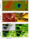 |
Fig. 1. Overview of the main sunspot, light bridge, penumbral filaments, and jets in AR 12741 on 2019 May 13. a–c: SDO/HMI LOS magnetogram, IRIS/SJI of 1400 Å, and SDO/AIA 171 Å image showing the magnetic fields of AR 12741 and the jets emanating from the west part of the light bridge within the main sunspot. The blue curves in (a) are contours of the LOS magnetogram at −1000 G and are duplicated to (b) and (c). The green dashed rectangle in (c) outlines the FOV of (d)–(g) and Figs. 2–6. d: NVST TiO image displaying the penumbral filaments, which intrude into the light bridge and sunspot umbrae. e–g: images of Hα line core and two wings (Δλ = ±0.5 Å) exhibiting two groups of jets (jet1 and jet2) emanating from the light bridge and brightenings near the jet bases (see the red contours). An animation (figure1.mov) of 1400 Å and 171 Å images, covering 00:51 UT to 01:51 UT, is available online. |
3.2. Footpoint brightenings and kinematic characteristics of the jets
As mentioned above, during the observed evolution of the jets, transient brightenings recurrently appeared around the jet base. Figures 2a1–a3 show these brightenings around 01:19 UT in NVST Hα blue wing, core, and red wing channels, respectively (also see the associated animation). Signatures of these brightenings can also be identified from simultaneous IRIS 1400 Å observations (see red contours in panel a4), indicating heating of local plasma to about 104.9 K. We note that this temperature is applicable only when the assumption of coronal equilibrium (CE) is valid (i.e., CHIANTI-based temperature) and may not be used for high-density atmospheres such as Ellerman bombs and UV bursts, where the formation temperature of IRIS Si IV lines could be 15 000–20 000 K (Rutten 2016; Toriumi et al. 2017). These transient brightenings recurred around the base region of jets, followed by ejection of the jets. The green dashed curves “Slice1” and “Slice2” in panel a3 approximately denote projected trajectories of jet1 and jet2 in the POS, respectively. Figures 2b1–b4 display the brightenings around 01:45 UT. Although these brightenings had weaker emission enhancement than those around 01:19 UT, they were scanned by the IRIS spectral slit at that time, which enables us to carry out a comprehensive spectral analysis.
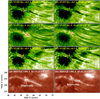 |
Fig. 2. Intermittent brightenings near the jet bases. a1–a4: NVST Hα blue wing image (Δλ = −0.5 Å), core image, red wing image (Δλ = +0.5 Å), and IRIS 1400 Å image showing the jets and associated brightenings (see the red contours) near the jet bases around 01:19 UT. The curves “Slice1” and “Slice2” in panel a3 approximate the projected trajectory of jet1 and jet2, respectively. b1–b4: similar to (a1)–(a4), but for the time point of 01:45 UT. An associated animation (figure2.mov) of Hα blue wing, core, and red wing images, covering 01:00 UT to 02:28 UT, is available online. |
To investigate the kinematic characteristics of jet1 and jet2, we derive time–distance plots from sequences of Hα images along the curves “Slice1” and “Slice2” in Fig. 2a3 and then display them in Figs. 3a1–a3 and b1–b3, respectively. The upward motions of the jets can be clearly seen in the Hα blue wing at −0.5 Å (panels a1 and b1), and downward motions are distinct in the Hα red wing at +0.5 Å (panels a3 and b3). Such kinematic characteristics of jets are also obviously revealed by the associated animation of Fig. 2. Here we focus on the upward motions of jet1 and jet2, and two rising phases of each jet are investigated in detail, onsets of which are marked by white dotted vertical lines. In the time–distance plots derived from Hα blue wing images, we track the jet front of each jet in the rising phase and record their y-axis coordinates at three time points with set intervals. After repeating the track processing five times, we get five groups of coordinates for the jet front in each rising phase. We then calculate the average values of these coordinates and plot three points at the time-distance plot for each ascending phase; the standard deviation is taken as the uncertainty. Finally, these points are fitted through the linear fitting, which is shown as a dotted oblique line in Figs. 3a1 and b1. The slope of the linear fitting line indicates the POS velocity of the jets. The projected ascending velocities of the front motions in the POS are 12.9 ± 0.6 km s−1 and 15.4 ± 0.6 km s−1 for jet1, and are 15.1 ± 0.5 km s−1 and 11.3 ± 0.6 km s−1 for jet2. Note that these POS velocities are measured at the late stage of the ascent, when the upward-ejecting jet fronts have decelerated from their peak velocities at the initial ascent stage. Furthermore, two downward flows are detected below the jet2 base with projected velocities of 10.7 ± 1.2 km s−1 and 9.5 ± 1.3 km s−1 (see panel b3). We can see that a base brightening accompanies some jet fronts (such as the first one of jet1) while no emission enhancement is visible around the jet bases for the other ones. This happens because the brightening regions around the jet bases are sometimes not crossed by “Slice1” or “Slice2”, but which are visible in the associated animation.
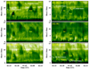 |
Fig. 3. Kinematic characteristics of the jets revealed by the NVST Hα observations. a1–a3: time–distance plots derived from the Hα blue wing, line core, and red wing images along the curve “Slice1” shown in Fig. 2a3. The dotted vertical lines mark the initial moments of two rising phases. The dotted oblique lines delineate linear fittings of the front of jet1 in two rising phases. b1–b3: similar to (a1)–(a3), but showing jet2 along the curve “Slice2”. |
By analyzing simultaneous observations from the IRIS, we find that the intermittent brightening around the jet bases in Hα channels can also be clearly detected in both the 1400 Å and 2796 Å images (see Figs. 4a1 and b1 and the associated animation). After the appearance of base brightening around 01:20 UT, a bright blob-like feature was observed in the 1400 Å channel (see the white arrows in panels a1–a3). The bright blob was ejected outward from the brightening site and moved along a POS trajectory similar to that of jet1 and jet2. The blue dashed curves (“Slice3”) in panels a3 and b3 approximate the POS trajectory of the bright blob, along which two time–distance plots are obtained from sequences of 1400 Å and 2796 Å images (see panels c1 and c2). The POS motion of the bright blob in the 1400 Å time–distance plot can be seen to accurately match a parabola consisting of an upward phase and a falling phase, which appears to be in the nature of true mass motion. Taking the same method used to estimate the POS velocities of the jet fronts in the Hα time–distance plot, we find that at the late stage of the ascent, the blob moved upward with a POS velocity of 11.9 ± 0.9 km s−1, and finally fell back. We note that the 1400 Å emission of the blob during the upward phase is obviously stronger than that in the falling phase, indicating local heating possibly caused by shock fronts or compression related to the upwardly ejecting material during the ascent phase (Hou et al. 2017; Tian et al. 2018). However, the 2796 Å time–distance plot of panel c2 reveals that the enhanced emission of the bright jet blob can only be identified during the period corresponding to the ascent phase in panel c1 with a POS velocity of 11.5 ± 0.9 km s−1 and that the trajectory is less distinct than that in the 1400 Å channel. As the IRIS 1400 Å and 2796 Å channels mainly sample the emission from plasma with different temperatures, these observations imply that the upwardly ejecting materials are multi-thermal. Moreover, the materials heated to the formation temperature of the 1400 Å channel could be accelerated enough to reach the height of the transition region and then fell back. However, the materials with lower temperatures corresponding to the 2796 Å channel would fall after they reached much lower heights, forming superimposed trajectories under a certain height.
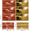 |
Fig. 4. Kinematic characteristics of the jets revealed by the IRIS observations. (a1)–(a3): sequence of 1400 Å images exhibiting the bright blob-like feature moving along the jet. The blue solid arrow in panel c denotes the ejecting direction of the bright blob. The dashed curve “Slice3” approximates the projected trajectory of bright blob. b1–b3: Corresponding 2796 Å images. (c1)–(c2): time-distance plots along the curve “Slice3” in 1400 Å and 2796 Å channels. The dotted oblique lines delineate linear fittings of projected trajectory of the bright blob in the rising phase. An animation (figure4.mov) of 1400 Å and 2796 Å channels, covering 00:40 UT to 01:51 UT, is available online. |
3.3. Spectral properties of the jets and the footpoint brightenings
From 01:42 UT to 01:51 UT, the IRIS spectrograph slit scanned our focused region. The slit crossed the brightening near the jet base around 01:43:58 UT (see green vertical dashed line in Fig. 5A). After that, the slit scanned the jet from east to west, and we select a slit position at 01:49:22 UT (see blue vertical dashed line) to investigate the spectral features of the jet. Panels B and C exhibit the detector images of C II 1334.53/1335.71 Å, Si IV 1393.76/1402.77 Å, and Mg II h&k 2796.35/2803.52 Å windows taken through the slit at the two positions shown in panel A. We average the spectra within a relatively quiet region around the jet-base brightening (see the black bars in panel A) and take the resultant profiles as reference profiles (see the black curves in panel D). Green and blue horizontal dashed lines in panels B and C indicate the locations where the slit crosses the jet-base brightening and jet. The profiles of UV emission lines of C II, Si IV, and Mg II ions measured along these two horizontal lines are exemplified by green and blue curves in panel D. It is obvious that compared with the reference profiles, the profiles sampled at the location of the jet-base brightening (green curves) are dramatically enhanced and remarkably broadened at both wings of each emission line. These features imply the existence of heating and bidirectional flows related to magnetic reconnections around the jet-base region (Peter et al. 2014; Tian et al. 2018). Another interesting feature of the jet-base brightening is that the Mg II 2798.809 Å line, which is actually a blend of 2798.754 Å and 2798.822 Å lines, changes from absorption to emission. Since the Mg II 2798.809 Å line emission can serve as a diagnostic for lower chromosphere heating (Pereira et al. 2015; Tian et al. 2015, 2016), this feature further demonstrates the occurrence of magnetic reconnections around the jet-base region. Furthermore, the profiles detected at the jet (blue curves) present a distinct intensity enhancement of the blue wings, indicating flows towards the observer along the LOS.
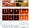 |
Fig. 5. IRIS spectral observations of the jets and jet-base brightening. A: IRIS 1400 Å and 2796 Å images. The green and blue vertical dashed lines mark the positions of the spectrograph slit at 01:43:58 UT and 01:49:22 UT, respectively. B–C: spectral Detector images taken through the spectrograph slit at the positions shown in (A). D: IRIS spectral line profiles along the green horizontal dashed line in (B) at the jet-base brightening and the blue line in (C) at the jet indicated by the arrows in (A). The reference line profiles are obtained by averaging the spectra within the section between the two black horizontal lines in (B) (also see the black bars in (A)). Here the intensities of profiles in the Mg II window are all divided by ten. |
To calculate the exact LOS velocity of the jets, we analyze the IRIS Si IV 1402.77 Å line profile. At 01:43:09 UT, the IRIS spectrograph slit was located at the east of the jet-base brightening and crossed the bases of jet1 and jet2 observed in Hα channels (see the blue and red plus symbols in Fig. 6a1). At the two crossing positions, obvious redshift signals are exhibited in the Si IV line spectra of panel a2. The red and blue plus symbols in panel a3 delineate the observed Si IV 1402.77 Å profiles sampled along the red and blue lines shown in panel a2. Since the observed Si IV profiles are close to Gaussian distribution, we apply single-Gaussian fitting to approximate the line profile (see the red and blue solid curves in panel a3). The Gaussian fit to the Si IV line profile is obtained by computing a nonlinear least-squares fit to a Gaussian function f(x) with three parameters:  , where
  . The three parameters represent the height of the Gaussian (A0), the center of the Gaussian (A1), and the width of the Gaussian (A2), respectively. We then obtain the Doppler velocity and its uncertainty according to the center of the Gaussian (A1) and its 1-sigma error estimate (Li et al. 2016; Zhang et al. 2018a). The Doppler velocities at the blue and red plus symbol positions are 9.7 ± 0.5 km s−1 and 13.0 ± 0.9 km s−1, indicating downward flows at the east of the base brightening of jet1 and jet2 (see blue and red dashed arrows in panel a1). At 01:50:43 UT, the scanning slit crossed the jet at a greater height, where jet1 and jet2 had merged into one jet flow (panel b1). The spectroscopic analysis reveals that there is a significant blueshift signal of −13.5 ± 0.4 km s−1 at the crossing position (panels b2–b3), implying an upward flow (see the blue dashed arrow in panel b1).
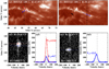 |
Fig. 6. Analysis of IRIS Si IV 1402.77 Å line for the jets with two directions. a1–a3: spectral analysis of the jets toward the solar surface. The black vertical line in (a1) marks the location of spectrograph slit at 01:43:41 UT, and the arrows denote the directions of downward jet flows cross the slit. Panel a2: Si IV 1402.77 Å line spectra along the slit. Panel a3: exhibits the Si IV 1402.77 Å line profiles (plus signs) and their single-Gaussian fitting profiles (solid curves) at positions indicated by the blue and red plus signs (dotted lines) shown in (a2). b1–b3: Similar to (a1)–(a3), but for the jets ejecting upward. |
3.4. Three-dimensional magnetic fields of the penumbral filaments revealed by NLFFF extrapolation
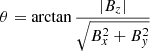
The kinematic characteristics of the jets ought to be deciphered for the magnetic fields of the intruding penumbral filaments and light bridge, which are further analyzed in Figs. 7 and 8. The NVST TiO image at 00:59:14 UT in Fig. 7a1 shows that, superposed on the west part of the light bridge, several penumbral filament intrusions penetrate into the umbrae from both sides. Each penumbral filament manifests as a dark core flanked by lateral brightenings. The corresponding photospheric vertical magnetic field is plotted as the background in panel a2, and the red arrows indicate the photospheric horizontal magnetic field around 01:00 UT. In the enlarged TiO image of panel b1, red arrows clearly depict strong photospheric horizontal fields (≃1000 G) along the penumbral filaments. At the east part of the light bridge, relatively weak and almost horizontal fields with an opposite direction are also detected. Furthermore, we compute the angle θ between the vector magnetic field and the horizontal plane as follows:
 (1)
(1)
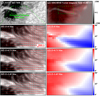 |
Fig. 7. Magnetic fields of the intruding penumbral filaments and sunspot light bridge. (a1)–(a2): NVST TiO image and SDO/HMI vector magnetogram showing the sunspot penumbral filaments intruding into umbrae at both sides of the light bridge and the corresponding photospheric magnetic fields. (b1)–(b3): enlarged TiO images superimposed by the horizontal magnetic fields (red arrows) calculated by NLFFF extrapolation at the height of z ≃ 0 Mm, z ≃ 0.73 Mm, and z ≃ 1.45 Mm, respectively. c1–c3: corresponding maps of the angle between the vector magnetic field and the horizontal plane. |
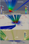 |
Fig. 8. 3D magnetic topology of the sunspot penumbral filaments intruding into the light bridge revealed by NLFFF extrapolation at 01:00 UT on 2019 May 13. Panels a and b: intruding filaments and sunspot umbral fields from a side view and a top view, respectively. Panel c: displays logarithmic Q distribution in the vertical plane based on the black cut denoted in (panel b), which distinctly depicts the high-Q region above the light bridge (LBQ). |
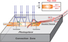 |
Fig. 9. Sketch illustrating the formation of the jets caused by the sunspot penumbral filament intrusions into the sunspot light bridge. The orange rectangle approximates mapping of the light bridge on the photosphere (indicated by the upper surface of a gray cube). The green curves represent emerging magnetic fields within the light bridge. Umbral magnetic fields surrounding the light bridge are denoted by the navy blue curves and resemble a magnetic canopy. The black curves delineate the magnetic fields of the penumbral filaments intruding into the umbrae on two sides of the light bridge. The star symbols mark the sites of magnetic reconnection. The red curves denote newly formed magnetic fields due to the reconnection occurring between the emerging fields within the light bridge and the highly inclined fields of the intruding filaments, along which downward flows and two groups of upward jets (jet1 and jet2) are observed. |
The θ map shown in panel c1 reveals that the sunspot umbrae have magnetic fields close to vertical (θ ≃ 90°) at the photospheric layer (Z ≃ 0 Mm), and the fields of sunspot penumbrae are more inclined (θ ≃ 45°). The magnetic fields of penumbral filaments intruding into the light bridge are almost horizontal (θ ≃ 0°). To reconstruct the 3D magnetic fields of AR 12741, we then perform NLFFF modeling based on the observed photospheric vector fields at 01:00 UT. Panels b2–c2 and b3–c3 display the extrapolated horizontal fields and θ maps at the height of Z ≃ 0.73 Mm and Z ≃ 1.45 Mm, respectively. Note that with the increase of altitude, the range of penumbral filament horizontal fields (deep blue region in the θ maps) keeps shrinking southwestward and gradually retreats from the light bridge. This indicates that, above the light-bridge region, the greater the height, the larger the θ value of the intruding filament fields. The southwest parts of the filaments, which are out of the light-bridge region, are dominated by inclined magnetic fields with smaller θ than surrounding penumbrae even at the height of Z ≃ 1.45 Mm.
For visualizations of the 3D magnetic topologies of our focused structures, we select a region from the NLFFF extrapolation and display it in Fig. 8. Moreover, we calculate the distributions of strength |B| and squashing factor Q of the reconstructed fields. Figures 8a and b show the sunspot umbral fields and intruding penumbral filaments from the side view and top view, respectively. The plotted field lines are colored depending on the local magnetic field strength (|B|). It is clear that there are highly inclined fields (stronger than 1000 G) intruding into the light bridge. These magnetic fields should correspond to the observed intruding penumbral filaments. In the Q map of the vertical plane above a cut crossing the light bridge (see black line in panel b), a high-Q region above the light bridge (LBQ) is visible (panel c), implying the existence of a magnetic canopy.
4. Summary and discussion
Based on high-quality observations from the NVST, SDO, and IRIS, we investigate an interesting event where several penumbral filaments intruded into a sunspot light bridge. On 2019 May 13, a light bridge completely separated the umbra of the main sunspot in AR 12741. The NVST TiO images show that superposed on the west part of the light bridge, several penumbral filaments intrude into the sunspot umbrae from both sides of the light bridge. Meanwhile, in IRIS 1400 Å and SDO/AIA 171 Å channels, bright jet-like activities were seen emanating from the west part of this light bridge. Similarly, the NVST Hα observations, especially at two wings of ±0.5 Å, reveal that two groups of jets (jet1 and jet2) originated from different sides of the light bridge and then approached each other when moving southwestward in the POS, which shared the same projected morphology with the intruding filaments. Additionally, intermittent brightenings and downward flows were detected around the jet bases. The IRIS spectral observations also provide convincing evidence of the presence of magnetic-reconnection-related heating and bidirectional flows near the jet-base region. Moreover, the IRIS SJIs of 1400 Å and spectral observations of 1402.77 Å line reveal that at the formation height of the 1402.77 Å line, the jets ejected southwestward in the POS had a POS velocity of 11.9 ± 0.9 km s−1 around 01:20 UT, and the LOS velocity was estimated as 13.5 ± 0.4 km s−1 at 01:50 UT. In the aspect of magnetic topology, the observed photospheric magnetic fields and extrapolated 3D fields reveal the existence of strong and highly inclined magnetic fields along the intruding penumbral filaments.
The jets reported in the present work can be observed in Hα, 1400 Å, and 171 Å channels, indicating that the jets consist of multi-thermal components. Moreover, the jets are accompanied by intermittent brightenings around the bases, which are clearly visible in the 1400 Å and 2796 Å images. This means that the local material at the jet-base region is heated to at least 104.0 K. In addition, the IRIS spectral profiles of the jet-base brightening are significantly enhanced and broadened at both wings of each emission line. These features are very similar to the recent IRIS observation of brightening events and are interpreted as local heating of plasma via magnetic reconnection and bidirectional outflows from the reconnection region (Peter et al. 2014; Toriumi et al. 2015a, 2017; Tian et al. 2016, 2018; Huang et al. 2018; Young et al. 2018; Chen et al. 2019). Moreover, the Mg II 2798.809 Å line of the jet-base brightening changes from absorption to emission. In solar spectra, the Mg II 2798.809 Å line is seen mostly in absorption, but can become an emission line when strong heating takes place in the lower chromosphere (Pereira et al. 2015; Tian et al. 2015, 2016; Toriumi et al. 2017). Therefore, it is highly possible that the profiles shown in Fig. 5 indicate the energy release caused by magnetic reconnection at the jet-base region. It is worth mentioning that reconnection is not the only mechanism that can lead to broadening of the spectra line. Currents, for instance, can also produce dissipation that can yield similar spectral shapes. However, the intensities of the spectra lines analyzed in this work are so strong that they cannot be mainly caused by the currents. Furthermore, the strong enhancements to both blue and red wings may not be explained merely by the Joule dissipation. As a result, we propose that the studied southwestward jets in the POS are likely outflows in one direction caused by the reconnection occurring around the jet bases. This interpretation is further supported by the downward flows displayed in Fig. 3b3, which may represent the outflow toward another direction.
In Fig. 3, we estimate the projected ascending velocities of the jets through the time–distance plot of Hα observations and obtain the values of 12.9 ± 0.6 km s−1, 15.4 ± 0.6 km s−1, 15.1 ± 0.5 km s−1, and 11.3 ± 0.6 km s−1 at different time points. However, for a vector velocity of the jets, we need to obtain the LOS component of true velocity, which can be measured by the IRIS spectral observations. Around 01:20 UT, jets were observed accompanied by distinct footpoint brightenings in both Hα and 1400 Å channels. Figure 4 reveals that a bright jet blob feature detected in IRIS 1400 Å channel moved southwestward with a POS velocity of about 11.9 km s−1, which is comparable to the value of 12.9 ± 0.6 km s−1 calculated based on the NVST Hα observations. However, due to the 320-step raster mode of the IRIS spectrograph slit, the LOS velocity of the jet can only be obtained when the scanning slit crossed the jet after 01:45 UT, whereas the POS motion of the jet was not distinct in the 1400 Å slit-jaw images but clear in H-alpha blue wing observations (second jet in Fig. 3a1). Therefore, for the jet around 01:50 UT shown in Fig. 6, which had a LOS velocity of ∼13.5 km s−1 estimated through the Doppler shift of the Si IV 1402.77 Å line, we adopt the POS velocity (∼15.4 km s−1) derived from the H-alpha observations as an approximation to that in the 1400 Å observations. As a result, we estimate the true velocity of the jet to be about 20.5 km s−1. Considering that the velocity is measured during the late stage of the ascent near the transition region, where the upward jets have been significantly decelerated by the solar effective gravity or resistance from the upper atmosphere, the estimated value should be the lower limit value of the initial speed of the upward jets when they are launched from a lower height, e.g., upper photosphere or lower chromosphere. That is, the peak velocity of the jet at the initial ascent stage should be much larger than 20.5 km s−1.
If we assume a proton number density (n) of 1015 cm−3 and a magnetic field strength (B) of 500 Gauss near the lower chromosphere above the sunspot light bridge, the Alfvén speed (VA) could be estimated to be ∼34.5 km s−1 according to the formula 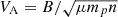 . Since the estimated Alfvén speed is not significantly larger than the lower limit value (20.5 km s−1) of the initial speed of the observed jets, it is reasonable to suggest that these jets are produced by magnetic reconnection near the lower solar atmosphere above the light bridge. Additionally, at the temperature of the lower solar atmosphere (∼10 000 K), the local sound speed (Cs ≃ 152T1/2 m s−1) could be estimated as ∼15.2 km s−1, which is smaller than the speed of the observed jets. This further supports the hypothesis that the intensity enhancement of the jet during its upward phase shown in Fig. 4 is caused by reconnection-related shock heating. Moreover, the intermittent and aperiodic occurrences of these jets also exclude the possible role of the p-mode wave on driving the jets, which is often suggested to account for the oscillating light walls above light bridges with a dominant period of several minutes (Yang et al. 2015; Zhang et al. 2017; Hou et al. 2017; Tian et al. 2018). One may see from the time–distance plots in Fig. 3 that the jets have a parabolic trajectory with a typical lifetime of 10–20 min. These jets are very similar to the surges reported by Toriumi et al. (2015a) and Robustini et al. (2016), which are interpreted as results of repeated magnetic reconnection driven by magneto-convective evolution.
As modeled by Nakamura et al. (2012), the jets generated by magnetic reconnection tend to move along stronger magnetic fields because weaker fields have higher gas pressure in the initial equilibrium and hence result in the gas pressure gradient along the strong fields, accelerating the field-aligned plasma flow. As a result, it is reasonable that within sunspots, the surge-like activities reported earlier are all aligned with stronger and relatively vertical background sunspot (umbral or penumbral) fields, because that they are driven by the magnetic reconnection occurring either between emerging magnetic fields within the light bridge and background sunspot (umbral) fields (Shimizu et al. 2009; Robustini et al. 2016; Hou et al. 2017; Tian et al. 2018) or between the horizontal penumbral filament fields and background sunspot (penumbral) fields (Katsukawa et al. 2007b; Jurčák & Katsukawa 2008; Magara 2010). But in the present work, the studied jets have the same projected morphology as the highly inclined intruding penumbral filaments, whose fields are weaker than the background sunspot fields but stronger than the emerging fields within the light bridge. We therefore propose that these jets could be driven by the magnetic reconnection between emerging fields within the light bridge and the intruding filament horizontal fields, and are then ejected outward along the stronger filament fields. As a result, the answers to the two questions raised in Sect. 1 would be that if penumbral filaments intrude into the light bridge, magnetic reconnection could occur between the emerging fields within the light bridge and penumbral filament fields, leading to jets being produced along the stronger filament fields.
Penumbral filaments and light bridges are dominant radial structures in the sunspot penumbra and remarkable bright lanes dividing the sunspot umbrae, respectively. The penumbral filaments are observed to have highly inclined or horizontal magnetic fields (Louis et al. 2014b). And the curved filamentary structures are present in some light bridges (Rimmele 2008). By analyzing high-resolution observations from the Swedish 1m Solar Telescope, SDO, and Hinode, Robustini et al. (2016) reported fan-shaped jets above the light bridge of a sunspot driven by reconnection and noticed that this light bridge exhibits a filamentary structure somewhat similar to the penumbral filament intrusions. However, due to the lack of high-resolution TiO observations, the emission features and morphologies of the filamentary structures within the light bridge and their relations to the fan-shaped jets cannot be investigated in detail. In the present work, with the help of high-resolution NVST TiO observations, we clearly show that the filamentary structures within the light bridge here have typical penumbral filament features of dark cores flanked by lateral brightenings (Scharmer et al. 2002). These filaments emanate from the sunspot penumbra, intrude into the light bridge, and then form two groups of penumbral intrusions, whose tips penetrate into the sunspot umbrae from both sides of the light bridge (see Figs. 1d and 7a1). The photospheric vector magnetic fields observed by SDO/HMI reveal that the intruding penumbral filaments have strong horizontal magnetic fields (≃1000 G) at the photospheric layer (see Figs. 7b1 and c1). Moreover, the NLFFF extrapolation results also provide solid evidence for the existence of highly inclined magnetic fields of the penumbral filaments at higher positions above the photosphere (see Figs. 7b2–c3 and 8). It can be estimated that near the transition region, that is, at the formation height of the 1402.77 Å line, the angle θ between the penumbral filament field and the horizontal plane is 30°–50°. Based on the position of the jets on the solar disk and the POS and LOS velocities of jets measured through the IRIS 1402.77 Å spectral imaging observations, we can calculate the angle φ between the jets and the local horizontal plane by applying the method of transforming the observed magnetic field vector in the image plane into the heliographic plane (Hagyard 1987; Gary & Hagyard 1990). The angle φ between the moving direction of the jets and the local horizontal plane at the formation height of the 1402.77 Å line is estimated to be ∼40°, which is highly consistent with the magnetic topology of the penumbral filaments. These results further reinforce our conclusion that the jets emanating from the light bridge are moving along the fields of the penumbral filaments.
To illustrate the magnetic fields of intruding penumbral filaments and light bridge as well as the formation process of the jets detected by the NVST, SDO, and IRIS, we draw a cartoon map and show it in Fig. 9. Within the light bridge (see the orange rectangle), low-lying magnetic structures (see the green curves) continuously emerge through long-lasting convection upflows from the solar interior to the solar atmosphere (Lites et al. 1991; Rueedi et al. 1995; Leka 1997; Jurčák et al. 2006; Rouppe van der Voort et al. 2010; Toriumi et al. 2015a,b; Zhang et al. 2018b). They are then restricted in the lower solar atmosphere by the above strong umbral fields (see the blue curves), which form a magnetic canopy covering the light bridge (Jurčák et al. 2006). When part of these emerging fields meet the overlying magnetic canopy field with opposite polarity at one side, current sheets are formed, leading to magnetic reconnection (see the stars at the east part of the light bridge) in the lower atmosphere (Asai et al. 2001; Shimizu et al. 2009; Hou et al. 2017; Tian et al. 2018). The resultant brightenings can be detected in Hα, 1400 Å, and 2796 Å channels in this event (see the animations attached to Figs. 1, 2, and 4). At the west part of the light bridge, the nearly horizontal fields of penumbral filaments (see the black curves) protrude into the light bridge. When the horizontal components of the emerging fields within the light bridge and filament fields are in opposite directions, current sheets will be formed. Subsequently, the vigorous convective upflows within the light bridge will push field lines with opposite directions together at the current sheets, giving rise to repeated magnetic reconnections between the horizontal filament fields and the emerging fields within the light bridge. The newly formed filament fields through reconnection are marked by the red curves and their footpoints within the sunspot keep moving from the umbrae into the light bridge, which is also confirmed by the evolution of the intruding penumbral filaments observed by the NVST. The repeated reconnections cause the observed intermittent brightenings while the reconnection outflows with opposite directions are observed as upward jet1 and jet2 along the filament fields and downward flows below the reconnection sites. From the top view, these outflows form a Y-shaped structure lying on the solar surface.
We highlight the fact that due to the lack of high-resolution observations of vector magnetic fields, such as the Hinode data, here we cannot find direct evidence of the emerging magnetic fields within the light bridge. However, emergence of magnetic flux within the light bridge has been widely demonstrated in recent observational and numerical works (Louis et al. 2015; Toriumi et al. 2015a,b; Yuan & Walsh 2016; Tian et al. 2018; Durán et al. 2020). Furthermore, some may wonder how, within the same light bridge, magnetic reconnection can trigger jets in some locations (the west part of the light bridge in the reported event) but not in others (the east part). We speculate that this could be influenced by the overlying magnetic topology and the occurrence height of the reconnection (deciding the surrounding plasma density), which we plan to investigate in detail in further work.
Similar to our observations, Yang et al. (2019a) reported that at the edge of a light bridge, light bridge filaments intruded into the sunspot umbrae. Nevertheless, the difference is that, around the tips of the intruding filaments, photospheric vortices and vertically launched jets were detected by Yang et al. (2019a). These authors considered that the strong transverse velocity shear between the light bridge and the umbrae triggered the Kelvin-Helmholtz instability (KHI) resulting in the vortex structures, which then launched the jet in the vertical direction through magnetic reconnection or waves. To our knowledge, velocity shear larger than (it would be twice under certain assumptions) the local Alfvén speed (here ∼10 km s−1 in the photosphere) is needed for KHI to take place (Chandrasekhar 1961; Li et al. 2019). Also, the KHI-induced vortices would form randomly at the boundary of flows (here the boundary is the edge of the light bridge). Considering the actual observations in both events reported in Yang et al. (2019a) and our study, we speculate that the vortices could be caused by the interaction between the large-scale, long-lasting horizontal flows and some small-scale local convection cells (Toriumi et al. 2015a) at some sites of the bridge during its developing phase, when the local convections are stronger than those in the mature (or decaying) bridges. The diverging flows caused by the small-scale local convection would block the large-scale horizontal flows along the bridge filaments at some sites and squeeze them (and the magnetic fields) outwards, which would then simultaneously intrude into the umbrae and form the vortex structures at both sides of the bridge. Subsequently, the horizontal intruding filament fields would reconnect with the vertical umbral fields and produce jets along the stronger vertical umbral fields. However, for the mature light bridge reported in our study, we suggest that the small-scale local convections are not strong enough to keep pushing the filaments. Therefore, the intruding filaments observed here would be much less active than that in Yang et al. (2019a) and would not reconnect with the umbral fields. On the other hand, random flux emergence caused by the weak local convection within the light bridge would interact with the above horizontal filament fields, producing jets ejecting outward along the stronger filaments fields. During the observation period of our event, we cannot find vertical jets in the light bridge, but we believe that during the developing phase of the light bridge, when the small-scale local convections are strong, the reconnection with the umbral field could be frequent, and thus vertical jets would be observed.
The magnetic fields of sunspot penumbra have been extensively investigated through observations of spectral lines forming in the photosphere and numerical simulations, which indicate horizontal magnetic fields along dark penumbral filaments and more vertical fields in the surrounding regions of penumbra (Thomas et al. 2002; Langhans et al. 2005; Scharmer et al. 2008; Rempel et al. 2009). Scharmer et al. (2002) presented the first observations of penumbral filaments with clear dark cores. Spruit & Scharmer (2006) introduced the concept of field-free convection gaps to explain the penumbral filaments, and a strong horizontal magnetic field was predicted to exist along the penumbral filament. The analysis presented here sheds light on the magnetic fields of the sunspot penumbral filament and light bridge, as well as the interactions between them. It is revealed that the fields of the penumbral filaments intruding into the sunspot light bridge and umbrae are indeed nearly horizontal at the photosphere and highly inclined at higher layers, which is depicted by the jets along these filaments observed in NVST Hα images. The interpretation of the formation of these jets mentioned above indicates that magnetic reconnection could occur between the penumbral filament fields and emerging fields within the light bridge, resulting in jets along the stronger filament fields. These results further complement the study of magnetic reconnection and dynamic activity within the sunspot.
Movies
Movie of Fig. 1 Access Supplementary Material
Movie of Fig. 2 Access Supplementary Material
Movie of Fig. 4 Access Supplementary Material
Acknowledgments
The authors appreciate the anonymous referee for the valuable suggestions. Y.H. thanks Prof. Hui Tian, Dr. Xiaoshuai Zhu, Dr. Yongliang Song, and Dr. Shuo Yang for helpful discussions. The data are used courtesy of NVST, SDO, and IRIS science teams. SDO is a mission of NASA’s Living With a Star Program. IRIS is a NASA small explorer mission developed and operated by LMSAL with mission operations executed at NASA Ames Research center and major contributions to downlink communications funded by ESA and the Norwegian Space Centre. The authors are supported by the National Key R&D Program of China (2019YFA0405000), the National Natural Science Foundation of China (11533008, 11903050, 11773039, 11790304, 11873059, 11673035, 11673034, and 11790300), the Strategic Priority Research Program of the Chinese Academy of Sciences (XDB41000000), the NAOC Nebula Talents Program, the Youth Innovation Promotion Association of CAS, Young Elite Scientists Sponsorship Program by CAST (2018QNRC001), and Key Programs of the Chinese Academy of Sciences (QYZDJ-SSW-SLH050).
References
- Asai, A., Ishii, T. T., & Kurokawa, H. 2001, ApJ, 555, L65 [NASA ADS] [CrossRef] [Google Scholar]
- Bai, X., Socas-Navarro, H., Nóbrega-Siverio, D., et al. 2019, ApJ, 870, 90 [CrossRef] [Google Scholar]
- Beckers, J. M., & Schröter, E. H. 1968, Sol. Phys., 4, 303 [NASA ADS] [CrossRef] [Google Scholar]
- Berger, T. E., & Berdyugina, S. V. 2003, ApJ, 589, L117 [NASA ADS] [CrossRef] [Google Scholar]
- Bharti, L. 2015, MNRAS, 452, L16 [NASA ADS] [CrossRef] [Google Scholar]
- Bharti, L., Solanki, S. K., & Hirzberger, J. 2017, A&A, 597, A127 [CrossRef] [EDP Sciences] [Google Scholar]
- Bobra, M. G., Sun, X., Hoeksema, J. T., et al. 2014, Sol. Phys., 289, 3549 [NASA ADS] [CrossRef] [Google Scholar]
- Borrero, J. M., & Ichimoto, K. 2011, Liv. Rev. Sol. Phys., 8, 4 [Google Scholar]
- Chandrasekhar, S. 1961, International Series of Monographs on Physics (Oxford: Clarendon) [Google Scholar]
- Chen, Y., Tian, H., Peter, H., et al. 2019, ApJ, 875, L30 [NASA ADS] [CrossRef] [Google Scholar]
- De Pontieu, B., Title, A. M., Lemen, J. R., et al. 2014, Sol. Phys., 289, 2733 [NASA ADS] [CrossRef] [Google Scholar]
- Drews, A., & Rouppe van der Voort, L. 2017, A&A, 602, A80 [NASA ADS] [CrossRef] [EDP Sciences] [Google Scholar]
- Durán, J. S. C., Lagg, A., Solanki, S. K., et al. 2020, ApJ, 895, 129 [CrossRef] [Google Scholar]
- Esteban Pozuelo, S., de la Cruz Rodríguez, J., Drews, A., et al. 2019, ApJ, 870, 88 [NASA ADS] [CrossRef] [Google Scholar]
- Felipe, T., Collados, M., Khomenko, E., et al. 2016, A&A, 596, A59 [NASA ADS] [CrossRef] [EDP Sciences] [Google Scholar]
- Felipe, T., Collados, M., Khomenko, E., et al. 2017, A&A, 608, A97 [CrossRef] [EDP Sciences] [Google Scholar]
- Goodarzi, H., Koutchmy, S., & Adjabshirizadeh, A. 2018, ApJ, 860, 168 [CrossRef] [Google Scholar]
- Gough, D. O., & Tayler, R. J. 1966, MNRAS, 133, 85 [NASA ADS] [CrossRef] [Google Scholar]
- Gary, G. A., & Hagyard, M. J. 1990, Sol. Phys., 126, 21 [NASA ADS] [CrossRef] [Google Scholar]
- Guglielmino, S. L., Romano, P., & Zuccarello, F. 2017, ApJ, 846, L16 [NASA ADS] [CrossRef] [Google Scholar]
- Guglielmino, S. L., Romano, P., Ruiz Cobo, B., Zuccarello, F., & Murabito, M. 2019, ApJ, 880, 34 [CrossRef] [Google Scholar]
- Hagyard, M. J. 1987, Sol. Phys., 107, 239 [NASA ADS] [CrossRef] [Google Scholar]
- Hou, Y., Zhang, J., Li, T., et al. 2016a, ApJ, 829, L29 [NASA ADS] [CrossRef] [Google Scholar]
- Hou, Y. J., Li, T., Yang, S. H., & Zhang, J. 2016b, A&A, 589, L7 [NASA ADS] [CrossRef] [EDP Sciences] [Google Scholar]
- Hou, Y., Zhang, J., Li, T., et al. 2017, ApJ, 848, L9 [CrossRef] [Google Scholar]
- Hou, Z., Huang, Z., Xia, L., et al. 2018, ApJ, 855, 65 [CrossRef] [Google Scholar]
- Huang, Z., Xia, L., Nelson, C. J., et al. 2018, ApJ, 854, 80 [CrossRef] [Google Scholar]
- Ichimoto, K., Suematsu, Y., Tsuneta, S., et al. 2007, Science, 318, 1597 [NASA ADS] [CrossRef] [PubMed] [Google Scholar]
- Jurčák, J., & Katsukawa, Y. 2008, A&A, 488, L33 [NASA ADS] [CrossRef] [EDP Sciences] [Google Scholar]
- Jurčák, J., Martínez Pillet, V., & Sobotka, M. 2006, A&A, 453, 1079 [NASA ADS] [CrossRef] [EDP Sciences] [Google Scholar]
- Katsukawa, Y., & Jurčák, J. 2010, A&A, 524, A20 [NASA ADS] [CrossRef] [EDP Sciences] [Google Scholar]
- Katsukawa, Y., Yokoyama, T., Berger, T. E., et al. 2007a, PASJ, 59, S577 [NASA ADS] [CrossRef] [Google Scholar]
- Katsukawa, Y., Berger, T. E., Ichimoto, K., et al. 2007b, Science, 318, 1594 [NASA ADS] [CrossRef] [Google Scholar]
- Kleint, L., & Sainz Dalda, A. 2013, ApJ, 770, 74 [NASA ADS] [CrossRef] [Google Scholar]
- Lagg, A., Solanki, S. K., van Noort, M., et al. 2014, A&A, 568, A60 [NASA ADS] [CrossRef] [EDP Sciences] [Google Scholar]
- Langhans, K., Scharmer, G. B., Kiselman, D., et al. 2005, A&A, 436, 1087 [NASA ADS] [CrossRef] [EDP Sciences] [Google Scholar]
- Langhans, K., Scharmer, G. B., Kiselman, D., et al. 2007, A&A, 464, 763 [NASA ADS] [CrossRef] [EDP Sciences] [Google Scholar]
- Leka, K. D. 1997, ApJ, 484, 900 [NASA ADS] [CrossRef] [Google Scholar]
- Lemen, J. R., Title, A. M., Akin, D. J., et al. 2012, Sol. Phys., 275, 17 [Google Scholar]
- Li, T., Yang, K., Hou, Y., & Zhang, J. 2016, ApJ, 830, 152 [NASA ADS] [CrossRef] [Google Scholar]
- Li, X., Zhang, J., Yang, S., et al. 2019, ApJ, 875, 52 [CrossRef] [Google Scholar]
- Lites, B. W., Bida, T. A., Johannesson, A., & Scharmer, G. B. 1991, ApJ, 373, 683 [NASA ADS] [CrossRef] [Google Scholar]
- Liu, R., Kliem, B., Titov, V. S., et al. 2016, ApJ, 818, 148 [Google Scholar]
- Liu, Z., Xu, J., Gu, B.-Z., et al. 2014, Res. Astron. Astrophys., 14, 705 [Google Scholar]
- Louis, R. E., Beck, C., & Ichimoto, K. 2014a, A&A, 567, A96 [NASA ADS] [CrossRef] [EDP Sciences] [Google Scholar]
- Louis, R. E., Beck, C., Mathew, S. K., et al. 2014b, A&A, 570, A92 [NASA ADS] [CrossRef] [EDP Sciences] [Google Scholar]
- Louis, R. E., Bellot Rubio, L. R., de la Cruz Rodríguez, J., Socas-Navarro, H., & Ortiz, A. 2015, A&A, 584, A1 [NASA ADS] [CrossRef] [EDP Sciences] [Google Scholar]
- Magara, T. 2010, ApJ, 715, L40 [NASA ADS] [CrossRef] [Google Scholar]
- Morton, R. J. 2012, A&A, 543, A6 [NASA ADS] [CrossRef] [EDP Sciences] [Google Scholar]
- Muller, R. 1973, Sol. Phys., 32, 409 [NASA ADS] [CrossRef] [Google Scholar]
- Muller, R. 1979, Sol. Phys., 61, 297 [NASA ADS] [CrossRef] [Google Scholar]
- Nakamura, N., Shibata, K., & Isobe, H. 2012, ApJ, 761, 87 [NASA ADS] [CrossRef] [Google Scholar]
- Pereira, T. M. D., Carlsson, M., De Pontieu, B., et al. 2015, ApJ, 806, 14 [NASA ADS] [CrossRef] [Google Scholar]
- Pesnell, W. D., Thompson, B. J., & Chamberlin, P. C. 2012, Sol. Phys., 275, 3 [Google Scholar]
- Peter, H., Tian, H., Curdt, W., et al. 2014, Science, 346, 1255726 [Google Scholar]
- Reardon, K., Tritschler, A., & Katsukawa, Y. 2013, ApJ, 779, 143 [NASA ADS] [CrossRef] [Google Scholar]
- Rempel, M., Schüssler, M., & Knölker, M. 2009, ApJ, 691, 640 [NASA ADS] [CrossRef] [Google Scholar]
- Riethmüller, T. L., Solanki, S. K., & Lagg, A. 2008, ApJ, 678, L157 [NASA ADS] [CrossRef] [Google Scholar]
- Rimmele, T. R. 1997, ApJ, 490, 458 [NASA ADS] [CrossRef] [Google Scholar]
- Rimmele, T. 2008, ApJ, 672, 684 [NASA ADS] [CrossRef] [Google Scholar]
- Robustini, C., Leenaarts, J., de la Cruz Rodriguez, J., & van der Rouppe Voort, L. 2016, A&A, 590, A57 [NASA ADS] [CrossRef] [EDP Sciences] [Google Scholar]
- Rouppe van der Voort, L., & de la Cruz Rodríguez, J. 2013, ApJ, 776, 56 [CrossRef] [Google Scholar]
- Rouppe van der Voort, L. H. M., & Drews, A. 2019, A&A, 626, A62 [CrossRef] [EDP Sciences] [Google Scholar]
- Rouppe van der Voort, L., Bellot Rubio, L. R., & Ortiz, A. 2010, ApJ, 718, L78 [NASA ADS] [CrossRef] [Google Scholar]
- Roy, J. R. 1973, Sol. Phys., 28, 95 [NASA ADS] [CrossRef] [Google Scholar]
- Rueedi, I., Solanki, S. K., & Livingston, W. 1995, A&A, 302, 543 [NASA ADS] [Google Scholar]
- Rutten, R. J. 2016, A&A, 590, A124 [NASA ADS] [CrossRef] [EDP Sciences] [Google Scholar]
- Ryutova, M., Berger, T., Frank, Z., et al. 2008, ApJ, 686, 1404 [NASA ADS] [CrossRef] [Google Scholar]
- Sakai, J. I., & Smith, P. D. 2008, ApJ, 687, L127 [NASA ADS] [CrossRef] [Google Scholar]
- Samanta, T., Tian, H., Banerjee, D., et al. 2017, ApJ, 835, L19 [NASA ADS] [CrossRef] [Google Scholar]
- Scharmer, G. B., Gudiksen, B. V., Kiselman, D., et al. 2002, Nature, 420, 151 [NASA ADS] [CrossRef] [PubMed] [Google Scholar]
- Scharmer, G. B., Narayan, G., Hillberg, T., et al. 2008, ApJ, 689, L69 [Google Scholar]
- Schlichenmaier, R., Jahn, K., & Schmidt, H. U. 1998, A&A, 337, 897 [NASA ADS] [Google Scholar]
- Schou, J., Scherrer, P. H., Bush, R. I., et al. 2012, Sol. Phys., 275, 229 [Google Scholar]
- Schüssler, M., & Vögler, A. 2006, ApJ, 641, L73 [NASA ADS] [CrossRef] [Google Scholar]
- Shimizu, T., Katsukawa, Y., Kubo, M., et al. 2009, ApJ, 696, L66 [NASA ADS] [CrossRef] [Google Scholar]
- Sobotka, M., Bonet, J. A., & Vazquez, M. 1994, ApJ, 426, 404 [NASA ADS] [CrossRef] [Google Scholar]
- Sobotka, M., Brandt, P. N., & Simon, G. W. 1997, A&A, 328, 682 [NASA ADS] [Google Scholar]
- Solanki, S. K. 2003, A&ARv., 11, 153 [Google Scholar]
- Spruit, H. C., & Scharmer, G. B. 2006, A&A, 447, 343 [NASA ADS] [CrossRef] [EDP Sciences] [Google Scholar]
- Su, J., Liu, Y., Zhang, H., et al. 2010, ApJ, 710, 170 [CrossRef] [Google Scholar]
- Thomas, J. H., Weiss, N. O., Tobias, S. M., et al. 2002, Nature, 420, 390 [NASA ADS] [CrossRef] [PubMed] [Google Scholar]
- Tian, H., Young, P. R., Reeves, K. K., et al. 2015, ApJ, 811, 139 [NASA ADS] [CrossRef] [Google Scholar]
- Tian, H., Xu, Z., He, J., et al. 2016, ApJ, 824, 96 [NASA ADS] [CrossRef] [Google Scholar]
- Tian, H., Yurchyshyn, V., Peter, H., et al. 2018, ApJ, 854, 92 [CrossRef] [Google Scholar]
- Titov, V. S., Hornig, G., & Démoulin, P. 2002, J. Geophys. Res. (Space Phys.), 107, 1164 [NASA ADS] [CrossRef] [Google Scholar]
- Tiwari, S. K., Moore, R. L., Winebarger, A. R., et al. 2016, ApJ, 816, 92 [NASA ADS] [CrossRef] [Google Scholar]
- Tiwari, S. K., van Noort, M., Lagg, A., et al. 2013, A&A, 557, A25 [NASA ADS] [CrossRef] [EDP Sciences] [Google Scholar]
- Toriumi, S., Katsukawa, Y., & Cheung, M. C. M. 2015a, ApJ, 811, 137 [NASA ADS] [CrossRef] [Google Scholar]
- Toriumi, S., Cheung, M. C. M., & Katsukawa, Y. 2015b, ApJ, 811, 138 [NASA ADS] [CrossRef] [Google Scholar]
- Toriumi, S., Katsukawa, Y., & Cheung, M. C. M. 2017, ApJ, 836, 63 [NASA ADS] [CrossRef] [Google Scholar]
- Wang, H., Liu, R., Li, Q., et al. 2018, ApJ, 852, L18 [CrossRef] [Google Scholar]
- Wheatland, M. S., Sturrock, P. A., & Roumeliotis, G. 2000, ApJ, 540, 1150 [Google Scholar]
- Wiegelmann, T. 2004, Sol. Phys., 219, 87 [NASA ADS] [CrossRef] [Google Scholar]
- Wiegelmann, T., Thalmann, J. K., Inhester, B., et al. 2012, Sol. Phys., 281, 37 [NASA ADS] [Google Scholar]
- Xiang, Y. Y., Liu, Z., & Jin, Z. Y., 2016, New Astron., 49, 8 [Google Scholar]
- Yang, S., Zhang, J., Jiang, F., & Xiang, Y. 2015, ApJ, 804, L27 [NASA ADS] [CrossRef] [Google Scholar]
- Yang, S., Zhang, J., & Erdélyi, R. 2016, ApJ, 833, L18 [NASA ADS] [CrossRef] [Google Scholar]
- Yang, S., Zhang, J., Erdélyi, R., et al. 2017, ApJ, 843, L15 [CrossRef] [Google Scholar]
- Yang, H., Lim, E.-K., Iijima, H., et al. 2019a, ApJ, 882, 175 [CrossRef] [Google Scholar]
- Yang, X., Yurchyshyn, V., Ahn, K., et al. 2019b, ApJ, 886, 64 [CrossRef] [Google Scholar]
- Young, P. R., Tian, H., Peter, H., et al. 2018, Space Sci. Rev., 214, 120 [NASA ADS] [CrossRef] [Google Scholar]
- Yuan, D., & Walsh, R. W. 2016, A&A, 594, A101 [CrossRef] [EDP Sciences] [Google Scholar]
- Zhang, J., Tian, H., He, J., & Wang, L. 2017, ApJ, 838, 2 [NASA ADS] [CrossRef] [Google Scholar]
- Zhang, B., Hou, Y. J., & Zhang, J. 2018a, A&A, 611, A47 [CrossRef] [EDP Sciences] [Google Scholar]
- Zhang, J., Tian, H., Solanki, S. K., et al. 2018b, ApJ, 865, 29 [CrossRef] [Google Scholar]
- Zhu, X., Wang, H., Cheng, X., et al. 2017, ApJ, 844, L20 [NASA ADS] [CrossRef] [Google Scholar]
All Figures
|
Fig. 1. Overview of the main sunspot, light bridge, penumbral filaments, and jets in AR 12741 on 2019 May 13. a–c: SDO/HMI LOS magnetogram, IRIS/SJI of 1400 Å, and SDO/AIA 171 Å image showing the magnetic fields of AR 12741 and the jets emanating from the west part of the light bridge within the main sunspot. The blue curves in (a) are contours of the LOS magnetogram at −1000 G and are duplicated to (b) and (c). The green dashed rectangle in (c) outlines the FOV of (d)–(g) and Figs. 2–6. d: NVST TiO image displaying the penumbral filaments, which intrude into the light bridge and sunspot umbrae. e–g: images of Hα line core and two wings (Δλ = ±0.5 Å) exhibiting two groups of jets (jet1 and jet2) emanating from the light bridge and brightenings near the jet bases (see the red contours). An animation (figure1.mov) of 1400 Å and 171 Å images, covering 00:51 UT to 01:51 UT, is available online. |
| In the text | |
|
Fig. 2. Intermittent brightenings near the jet bases. a1–a4: NVST Hα blue wing image (Δλ = −0.5 Å), core image, red wing image (Δλ = +0.5 Å), and IRIS 1400 Å image showing the jets and associated brightenings (see the red contours) near the jet bases around 01:19 UT. The curves “Slice1” and “Slice2” in panel a3 approximate the projected trajectory of jet1 and jet2, respectively. b1–b4: similar to (a1)–(a4), but for the time point of 01:45 UT. An associated animation (figure2.mov) of Hα blue wing, core, and red wing images, covering 01:00 UT to 02:28 UT, is available online. |
| In the text | |
|
Fig. 3. Kinematic characteristics of the jets revealed by the NVST Hα observations. a1–a3: time–distance plots derived from the Hα blue wing, line core, and red wing images along the curve “Slice1” shown in Fig. 2a3. The dotted vertical lines mark the initial moments of two rising phases. The dotted oblique lines delineate linear fittings of the front of jet1 in two rising phases. b1–b3: similar to (a1)–(a3), but showing jet2 along the curve “Slice2”. |
| In the text | |
|
Fig. 4. Kinematic characteristics of the jets revealed by the IRIS observations. (a1)–(a3): sequence of 1400 Å images exhibiting the bright blob-like feature moving along the jet. The blue solid arrow in panel c denotes the ejecting direction of the bright blob. The dashed curve “Slice3” approximates the projected trajectory of bright blob. b1–b3: Corresponding 2796 Å images. (c1)–(c2): time-distance plots along the curve “Slice3” in 1400 Å and 2796 Å channels. The dotted oblique lines delineate linear fittings of projected trajectory of the bright blob in the rising phase. An animation (figure4.mov) of 1400 Å and 2796 Å channels, covering 00:40 UT to 01:51 UT, is available online. |
| In the text | |
|
Fig. 5. IRIS spectral observations of the jets and jet-base brightening. A: IRIS 1400 Å and 2796 Å images. The green and blue vertical dashed lines mark the positions of the spectrograph slit at 01:43:58 UT and 01:49:22 UT, respectively. B–C: spectral Detector images taken through the spectrograph slit at the positions shown in (A). D: IRIS spectral line profiles along the green horizontal dashed line in (B) at the jet-base brightening and the blue line in (C) at the jet indicated by the arrows in (A). The reference line profiles are obtained by averaging the spectra within the section between the two black horizontal lines in (B) (also see the black bars in (A)). Here the intensities of profiles in the Mg II window are all divided by ten. |
| In the text | |
|
Fig. 6. Analysis of IRIS Si IV 1402.77 Å line for the jets with two directions. a1–a3: spectral analysis of the jets toward the solar surface. The black vertical line in (a1) marks the location of spectrograph slit at 01:43:41 UT, and the arrows denote the directions of downward jet flows cross the slit. Panel a2: Si IV 1402.77 Å line spectra along the slit. Panel a3: exhibits the Si IV 1402.77 Å line profiles (plus signs) and their single-Gaussian fitting profiles (solid curves) at positions indicated by the blue and red plus signs (dotted lines) shown in (a2). b1–b3: Similar to (a1)–(a3), but for the jets ejecting upward. |
| In the text | |
|
Fig. 7. Magnetic fields of the intruding penumbral filaments and sunspot light bridge. (a1)–(a2): NVST TiO image and SDO/HMI vector magnetogram showing the sunspot penumbral filaments intruding into umbrae at both sides of the light bridge and the corresponding photospheric magnetic fields. (b1)–(b3): enlarged TiO images superimposed by the horizontal magnetic fields (red arrows) calculated by NLFFF extrapolation at the height of z ≃ 0 Mm, z ≃ 0.73 Mm, and z ≃ 1.45 Mm, respectively. c1–c3: corresponding maps of the angle between the vector magnetic field and the horizontal plane. |
| In the text | |
|
Fig. 8. 3D magnetic topology of the sunspot penumbral filaments intruding into the light bridge revealed by NLFFF extrapolation at 01:00 UT on 2019 May 13. Panels a and b: intruding filaments and sunspot umbral fields from a side view and a top view, respectively. Panel c: displays logarithmic Q distribution in the vertical plane based on the black cut denoted in (panel b), which distinctly depicts the high-Q region above the light bridge (LBQ). |
| In the text | |
|
Fig. 9. Sketch illustrating the formation of the jets caused by the sunspot penumbral filament intrusions into the sunspot light bridge. The orange rectangle approximates mapping of the light bridge on the photosphere (indicated by the upper surface of a gray cube). The green curves represent emerging magnetic fields within the light bridge. Umbral magnetic fields surrounding the light bridge are denoted by the navy blue curves and resemble a magnetic canopy. The black curves delineate the magnetic fields of the penumbral filaments intruding into the umbrae on two sides of the light bridge. The star symbols mark the sites of magnetic reconnection. The red curves denote newly formed magnetic fields due to the reconnection occurring between the emerging fields within the light bridge and the highly inclined fields of the intruding filaments, along which downward flows and two groups of upward jets (jet1 and jet2) are observed. |
| In the text | |
Current usage metrics show cumulative count of Article Views (full-text article views including HTML views, PDF and ePub downloads, according to the available data) and Abstracts Views on Vision4Press platform.
Data correspond to usage on the plateform after 2015. The current usage metrics is available 48-96 hours after online publication and is updated daily on week days.
Initial download of the metrics may take a while.