| Issue |
A&A
Volume 641, September 2020
|
|
|---|---|---|
| Article Number | A161 | |
| Number of page(s) | 9 | |
| Section | Planets and planetary systems | |
| DOI | https://doi.org/10.1051/0004-6361/202038412 | |
| Published online | 24 September 2020 | |
Search for He I airglow emission from the hot Jupiter τ Boo b
1
Leiden Observatory, Leiden University,
Postbus 9513,
2300 RA
Leiden, The Netherlands
e-mail: This email address is being protected from spambots. You need JavaScript enabled to view it.
2
Max-Planck-Institut für Astronomie,
Königstuhl 17,
69117
Heidelberg, Germany
3
Department of Physics, University of Warwick,
Coventry
CV4 7AL, UK
4
INAF – Osservatorio Astrofisico di Torino,
Via Osservatorio 20,
10025
Pino Torinese, Italy
5
Centre for Exoplanets and Habitability, University of Warwick,
Gibbet Hill,
Coventry,
CV4 7AL, UK
6
Université Grenoble Alpes, CNRS, IPAG,
38000
Grenoble, France
Received:
13
May
2020
Accepted:
24
July
2020
Abstract
Context. It has been suggested that the helium absorption line at 10 830 Å that originates from the metastable triplet state 23S is an excellent probe for the extended atmospheres of hot Jupiters and their hydrodynamic escape processes. It has recently been detected in the transmission spectra of a handful of planets. The isotropic reemission will lead to helium airglow that may be observable at other orbital phases.
Aims. We investigate the detectability of He I emission at 10 830 Å in the atmospheres of exoplanets using high-resolution spectroscopy. This would provide insights into the properties of the upper atmospheres of close-in gas giants.
Methods. We estimated the expected strength of He I emission in hot Jupiters based on their transmission signal. We searched for the He I 10 830 Å emission feature in τ Boo b in three nights of high-resolution spectra taken by CARMENES at the 3.5m Calar Alto telescope. The spectra from each night were corrected for telluric absorption, sky emission lines, and stellar features, and were shifted to the planetary rest frame to search for the emission.
Results. The He I emission is not detected in τ Boo b at a 5σ contrast limit of 4 × 10⁻⁴ for emission line widths of >20 km s−1. This is about a factor 8 above the expected emission level (assuming a typical He I transit absorption of 1% for hot Jupiters). This suggests that targeting the He I emission with well-designed observations using upcoming instruments such as VLT/CRIRES+ and E-ELT/HIRES is possible.
Key words: planets and satellites: atmospheres / planets and satellites: individual: τ Boo b / techniques: spectroscopic / infrared: planetary systems
© ESO 2020
1 Introduction
The atmospheres of close-in exoplanets are strongly affected by the high-energy irradiation from their host stars, which causes their upper atmospheres to become weakly bound and susceptible to hydrodynamic escape (Owen 2019). For gas-giant planets, Lyman-α absorption in transit measurements has been the primary probe for their extended atmospheres, for instance, in HD 209458b (Vidal-Madjar et al. 2003), GJ 436b (Kulow et al. 2014; Ehrenreich et al. 2015), and GJ 3470b (Bourrier et al. 2018). Such observations trace the exospheres in which neutral hydrogen extends far beyond the Roche-lobe radius, and cast light on the hydrodynamic escape and mass loss that drives the evolution of the atmospheric and bulk composition of close-in exoplanets (Ehrenreich et al. 2015).
In addition to Lyα, helium at 10 830 Å was also identified to be a powerful tracer of the extended atmospheres (Seager & Sasselov 2000), which was recently reassessed by Oklopčić & Hirata (2018). This helium line has several advantages over Lyα because it is less strongly affected by interstellar absorption and can be observed from the ground with high-resolution spectrographs. This opens a new window into the characterization of exospheres.
The theoretical work by Oklopčić & Hirata (2018) has resulted in a breakthrough in helium measurements. Excess absorption was first detected by the Wide Field Camera 3 on board the Hubble Space Telescope in WASP-107b (Spake et al. 2018) and was independently confirmed by ground-based observations (Allart et al. 2019; Kirk et al. 2020) that showed an absorption level of 5.54 ± 0.27%. In addition, another five planets have been reported with helium signals: HAT-P-11b at a level of 1.08 ± 0.05% (Allart et al. 2018; Mansfield et al. 2018), HD 189733b at 0.88 ± 0.04% (Salz et al. 2018; Guilluy et al. 2020), WASP-69b at 3.59 ± 0.19% (Nortmann et al. 2018), HD 209458b at 0.91 ± 0.10% (Alonso-Floriano et al. 2019), and GJ 3470b at 1.5 ± 0.3% (Ninan et al. 2020; Palle et al. 2020). Upper limits in He I absorption were derived for Kelt-9b and GJ 436b at 0.33 and 0.41% (Nortmann et al. 2018), for WASP-12b at 59 ± 143 ppm over a70 Å band (Kreidberg & Oklopčić 2018), for GJ 1214b at 3.8% ± 4.3% (Crossfield et al. 2019), for K2-100b with an equivalent width (EW) smaller than 5.7 mÅ (Gaidos et al. 2020), and AU Mic b with an EW of 3.7 mÅ (Hirano et al. 2020).
The wide range of helium absorption levels seen in the transmission spectra of hot gas giants is likely due to the variety in the stellar radiation fields. The helium absorption line at 10 830 Å originates from atoms in a metastable triplet state 23 S, which is mainly populated through recombination of ionized helium. The ionization of He I requires photons with wavelengths smaller than 504 Å, that is, X-ray and extreme-ultraviolet (EUV). Therefore, the helium absorption is expected to be enhanced for planets irradiated with higher X-ray and EUV flux (Nortmann et al. 2018). However, the level of EUV irradiation may not be the only determining factor. The mid-UV radiation near 2600 Å can depopulate the triplet state 23S through ionization. The strength of the helium absorption has therefore been proposed to depend on the ratio between EUV and mid-UV stellar fluxes, and K-type stars may provide the most favorable stellar environment (Oklopčić 2019). The exoplanets with detected helium absorption generally support this trend so far; four out of six exoplanets orbit K-type stars. More detections will help to better understand the factors that affect the He I absorption level.
As helium atoms at the triplet state 23S absorb photons to reach the 23P state, the opposite transition will occur concurrently, in which 10 830 Å photons are reemitted in random directions. Based on the absorption level, we estimate the amount of emission expected from the planetary atmospheres. The study of He I airglow emission allows us to better understand the radiation fields and level populations under nonlocal thermodynamic equilibrium in the upper atmospheres. In addition, it provides a way of probing the extended atmospheres of nontransiting close-in gas giants, which have not been investigated before.
In this paper, we address the detectability of He I emission in the atmospheres of close-in exoplanets. We first calculate the expected emission level (Sect. 2), then perform a case study on τ Boo b (Sect. 3) by searching for helium airglow emission in high-resolution spectroscopic data from the Calar Alto high-Resolution search for M dwarfs with Exoearths with Near-infrared and optical Echelle Spectrographs (CARMENES) in Sects. 4 and 5. We discuss our results and future prospects in Sect. 6.
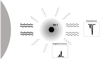 |
Fig. 1 Illustration of He I emission from an exosphere of a close-in planet. The gray disk represents the extended atmosphere around such a planet. He I absorption is observed during transit, while airglow emission can be probed at other orbital phases. |
2 Helium emission from extended atmospheres
The concept of probing He I airglow emission is illustrated in Fig. 1. We consider the extended atmosphere as an optically thin cloud surrounding the exoplanet. The cloud absorbs a fraction of irradiation from the host star due to the transition at 10 830 Å, which excites the helium atoms at state 23 S to the higher state 23P. The absorbed radiation is reemitted isotropically when the excited electrons return to the metastable triplet state. In the assumption that the extended atmosphere has a low density and is optically thin, the reemitted photons can freely escape and be observed as an emission feature. During transit, the feature is seen in absorption because only a small fraction of the radiation is reemitted along the line of sight. Consequently, we can detect He I absorption lines during transit and emission lines from other viewing angles.
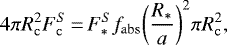
To estimate the strength of the He I emission, the cloud is assumed to absorb a fraction of the incident stellar energy at 10 830 Å and to reemit it isotropically. Assuming that the upper energy level is not (de-)populated in another way, we can estimate (see Seager 2010)
 (1)
(1)
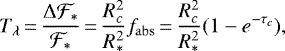
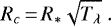
where Rc is the radius of the cloud that absorbs radiation at that wavelength, R* is the stellar radius, a is the orbital distance of the planet, fabs is the fraction of energy absorbed at 10 830 Å, which is linked to the column density of helium atoms at state 23 S in the cloud,  and
and  denotes the 10 830 Å flux at the surface of the planet and the star, respectively. The corresponding fluxes that we observe at Earth are
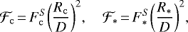 (2)
(2)
where D is the distanceof the system to Earth. Thus, the planet to star contrast at 10 830 Å is
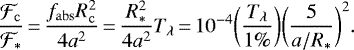 (3)
(3)
Tλ is the excess absorption at 10 830 Å that can be measured by transmission spectroscopy, with  .
.
The uncertainties regarding this estimate are further discussed in Sect. 6.1. A more detailed derivation involving radiative transfer is presented in Appendix A. Based on Eq. (3), we expect contrast levels of ~ 10−4, which may be reached by combining multiple nights of observations.
3 τ Boo system
The hot Jupiter τ Bootis b is one of the first exoplanets that has been discovered (Butler et al. 1997). It orbits a bright F7V type main-sequence star (V = 4.5 mag) at a distance of 15.6 pc from Earth. Although the planet is not transiting, its orbital inclination was determined to be 45° by tracking CO absorption in its thermal dayside spectrum (Brogi et al. 2012), which was confirmed by measurements of H2O (Lockwood et al. 2014). The properties of the τ Boo system are summarized in Table 1. Because the planet is not transiting, there is unfortunately no direct measure of its radius (meaning that its surface gravity is unknown), and the He I 10 830 Å line cannot be probed in transmission.
The system has been an interesting target for investigating star-planet interactions because of its strong stellar activity. The star has a high S-index of 0.202 (Wright et al. 2004), indicating strong emission cores in the Ca II H&K lines. It exhibits an X-ray luminosity of 9 × 1028 erg s−1 (Huensch et al. 1998) and a reconstructed EUV luminosity of 2.5 × 1029 erg s−1 (Sanz-Forcada et al. 2011), which are among the highest values found in the planet-hosting stars. The intense X-ray and EUV radiation can deposit substantial energy in the planetary atmosphere, facilitating the expansion and evaporation of gas. Although τ Boo is not a K-type star (which is probably the most favorable spectral type for probing the helium line), τ Boo b might well have an extended atmosphere with a large population of helium at the triplet state because its stellar X-ray and EUV emission is high, and it is a promising target to search for the He I emission at 10 830 Å.
Properties of the star τ Boo (upper part) and τ Boo b (lower part).
4 Observations and data analysis
We observed and analyzed the τ Boo system for five nights with the CARMENES spectrograph, which is mounted on the 3.5 m Calar-Alto Telescope (Quirrenbach et al. 2016), on 26 March2018, 11 May 2018, 12 March 2019, 15 March 2019, and 11 April 2019. CARMENES has two channels, VIS and NIR, that cover the optical wavelength range (520–960 nm) and the near-infrared (NIR) wavelength range (960–1710 nm), respectively. The resolving power is 94 600 in theVIS channel and 80 400 in the NIR channel. Each channel is fed with two fibers: fiber A targets the star, and fiber B simultaneously obtains a sky spectrum. The He I line at 10 830 Å falls on echelle order 56 (10 801–11 001 Å) in the NIR channel. We focus our analysis on this order.
The details of the observations are shown in Table 2 and Fig. 2. The observations probed thermal emission from τ Boo b, covering a wide range in planet orbital phases each night (see Fig. 2). The exposure times were adjusted according to the weather conditions, maintaining a signal-to-noise ratio (S/N) of ≥100. The observations in the first two nights were taken with exposure times of 40 s with a seeing of 2′′ and 1.4′′, delivering lower S/N per spectrum than during the other nights with longer exposures and better weather conditions. The drop-off in S/N at the end of night 2 was due to the increasingly high airmass. The relative humidity during nights 1, 2, and 5 continuously exceeded 85%, in contrast to the lower value (~45%) during night 4. This agrees well with the behavior of the S/N in these nights. Although the relative humidity was not as high as in the first two nights, it varied strongly in night 3, which might account for the drastic change in S/N.
The standard data reduction, such as bias removal, flat fielding, correction for cosmic-rays, and wavelength calibration, was performed with the CARMENES pipeline CARACAL v2.10 (Caballero et al. 2016). The output of the pipeline was provided in the observer frame with a vacuum wavelength solution. We converted the vacuum wavelength solution into air wavelengths and used it throughout our analysis.
4.1 Data analysis
First, we manually corrected for additional hot pixels and cosmic rays present in the pipeline-reduced spectra by substituting these values with the linear interpolation of adjacent pixels or adjacent time series. Subsequently, each spectrum was normalized to unity using the continuum at the blue and red side of the helium line over the ranges 10 804.0–10 805.2 Å, 10 818.5–10 819.0 Å, and 10 839.0–10 840.3 Å. After normalization, the spectral series of each night were handled as a two-dimensional matrix, as shown in Fig. 3a. Each row in the matrix represents one spectrum, and the frame number is given on the y-axis. The y-axis also corresponds to orbital phase or time.
Before correcting for the telluric lines, we first removed the stellar Si line and He I triplet at 10 827.1 Å and 10 829.09, 10 830.25, and 10 830.34 Å. In order to achieve this, we built an empirical stellar model for each night by combining all spectra with S/N > 100 in the stellar rest frame, where we set all values outside of the two stellar features to unity. This model was then shifted to the observer’s rest frame, was scaled, and then removed from each spectrum. Subsequently, the spectra were free of stellar lines in the wavelength region near the planetary helium line (see Fig. 3b).
The residual matrix in Fig. 3b shows the telluric lines near the planetary helium signal that required removal, including the H2O absorption features at 10 832.1 and 10 834.0 Å, and the OH emission lines at 10 824.7, 10 829.8, and 10 831.3 Å. The strengths of telluric lines vary overnight, which mainly results from the change in airmass and/or water column. To correct for telluric absorption lines, we measured the temporal variation of the flux at the centers of several deep H2O absorption features and combined them to serve as a representation for the atmospheric change overnight. This temporal variation was then removed using a column-by-column linear regression while avoiding the columns that contain the assumed planetary He I emission. We removed the sky emission lines in a similar way, using their mean-variation overnight. After telluric correction, each column of the matrix was subsequently normalized as follows. The spectra were combined via weighted average, with the weights defined as the squared S/N of each exposure, to build a master spectrum. Each individual spectrum was subsequently divided by this master spectrum to obtain the residual spectral series, as shown in Fig. 3c.
We note that during the telluric removal and final normalisation, we masked the region in each spectrum where the planetary He line is expected to appear, so that we were able to avoid self-subtraction of the signal, if present. This is particularly important ifthe planetary He I line is broad. When the line width is larger than the change in the planetary radial velocity overnight, the planetary signal would be (partially) subtracted out, making it less likely to be detected.
4.2 Additional noise in residual spectra
After correcting for the stellar and telluric effects, we shifted the residual spectral series of all five nights into the stellar rest frame by correcting for the systemic velocity, barycentric velocity, and stellar reflex motion of τ Boo, as shown in Fig. 4. The spectra were binned to 0.006 in phase (y-axis) for a better identification of the noise structure. We saw that the observations in nights 2 and 3 included broad noise structures, which may originate from the variability of stellar lines or the residuals of telluric corrections.
As we noted in Sect. 3, the chromosphere of τ Boo is highly active. The stellar He I line as a chromospheric diagnostic may undergo temporal variation due to flaring. The strength of the stellar He I line can also show periodic modulation by rotation if the line isnot homogeneous on the stellar disk (Andretta et al. 2017). Moreover, the fast spin of τ Boo may result in residual noise features that shift in wavelength up to its rotation velocity (~15 km s−1). To quantify the effect of stellar variability, we measured the strength of the stellar He I line at 10 830 Å during each night by fitting a Gaussian profile to the data and measuring the amplitude of the best-fit Gaussian profile. We define the line variation as the relative depth with respect to the average stellar spectrum of each night, and then bin the results to 0.006 in phase (see Fig. 2 bottom panel). During a single night, the variation is generally ≤0.25%, which is within the noise level of the data and therefore should not significantly affect our analysis. However, it is possible that the variation can build up as we combine different frames during the night, leading to systematic noise in the combined residual spectrum. For example, the variability of He I line may cause the variation in the residual fluxat 10 830.3 Å in night 2 (see Fig. 4). We also compared the average line profile of different nights (Fig. 5). On a night-to-night basis, we note that the helium line profile in night 2 is distinct from other nights, perhaps due to the effect of the nearby strong telluric line or the higher level of stellar activity.
In addition, we note that the spectral S/N in the middle of night 3 abruptly dropped by a factor of two, as shown in Fig. 2, probably due to the changing weather condition. This may lead to the inconsistency of the data in the region from 10 829.4 to 10 830.2 Å. Unfortunately, the trail of the planetary signal in night 3 resides exactly in this problematic wavelength range, which is crowded by artifacts (see Fig. 4). In the night 2 observations, telluric lines are very strong and variable because the relative humidity was high and the precipitable water vapor varied. We were unable to completely remove this. The residuals of the deep telluric H2O line at 10 832.1 Å and OH sky emission at 10 831.3 Å coincide with the trail of the planetary signal (see Fig. 4), which means that it is difficult to preserve it while removing the telluric contamination. In this condition, the S/N is not improved by adding the night 2 data because more noise was introduced along with the weaker signal. We therefore excluded the observations of night 2 and 3 from further analysis.
Based on the ephemeris listed in Table 1, we shifted the residual spectra to the planetary rest frame. The residual spectral series from different nights were then combined with each residual spectrum weighted by its variance over the radial velocity ranges from −150 to −50 km s−1 and from 50 to 150 km s−1.
Observation summary.
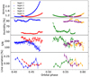 |
Fig. 2 Variation in airmass (upper panel), relative humidity (mid panel), S/N (lower panel) and variation around the mean of thestellar He I line (bottom panel) during observations in the different nights. The S/N of each spectrum is defined as the average signal-to-noise ratio of the continuum near the He I 10 830 Å line. |
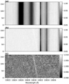 |
Fig. 3 Illustration of the data reduction steps we applied to the spectral series taken on night 4. Each row in the matrix represents one spectrum, and the y-axis corresponds to time. As detailed in Sect. 4.1, the steps include (a) normalization of the continuum, (b) correction for stellar lines in each spectrum using an empirical model, and (c) removal of telluric contamination by correcting the temporal variation of the flux in telluric lines using a column-by-column linear regression. The trail of an artificially injected planetary helium line (with a magnitude of 0.3% and a width of 11 km s−1) is visible as a slanted white band near 10 830 Å that shifts in time as a result of the change in the radial component of the orbital velocity of the planet. |
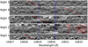 |
Fig. 4 Residual spectral series from nights 1 to 5. The y-axis represents the time or orbital phase. The residuals are binned to 0.006 in phase for clarity. The slanted dashed lines in red trace the expected planetary helium line. The dotted lines in blue denote the positions of the stellar He I triplet. The shaded region in night 2 contains the telluric H2O absorption and OH emission line, which overlap the expected planetary helium line. |
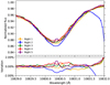 |
Fig. 5 Upper panel: average profile of the stellar helium line in each night. Lower panel: difference of each profile with respect to the mean. The deep absorption line at 10 832.2 Å in night 2 (blue curve) is a telluric H2O line. The small peaks on top of the helium line in night 1 and 5 are caused by sky OH emission. |
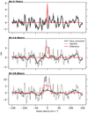 |
Fig. 6 Combined (three nights) residual spectra in the planetary rest frame centered at the 10 830 Å He I line. In the three panels, the solid black line indicates the residual spectra, boxcar-smoothed by 3.7 km s−1 (top), 14.9 km s−1 (middle), and 29.8 km s−1 (bottom). The dotted curves show an artificially injected signal at an S/N of 5, and the solid red curve shows the difference between the injectedand original data. The values are scaled by the standard deviation of the observed residuals so that the y-axis represents the S/N. |
5 Result
Figure 6 shows the time-averaged spectrum around the helium line in the planet rest-frame. The amplitude is scaled to make the standard deviation equal to unity around the targeted He I 10 830 Å line. We find no statistically significant signal from the planetary He I 10 830 Å line within the three nights of observations.
5.1 Detection limits
As we have no information on the profile of the potential He I line originating from τ Boo b, we assumed a box profile centered at 10 830.3 Å, which has a clear definition of the line width compared to a Gaussian profile. We performed signal injections considering various widths (W) of the planetary emission, ranging from 3.7 km s−1 (equal to the instrument resolution) to 37 km s−1 (which is limited by the self-subtraction of broad signals). The combined residuals of the observations and injections are shown in Fig. 6 for three different line widths as examples. We regarded the original residuals (without signal injection) as the noise, and convolved it with the corresponding signal profile to take the width of the signal into account. The noise level is defined as the standard deviation (from −150 to +150 km s−1) of the convolved residuals. These were then scaled by this noise level, so that the y-axis represents the S/N. The strength of the signal in each injection case was determined by measuring the amplitude of the recovered signal, which is the difference between the injected and the original residuals, as shown by the red curves in Fig. 6. The 5σ detection limits were thus determined as the minimum line emission leading to a recovered S/N of 5 in our injection tests. The detection limit as a function of the line width is shown in Fig. 7. We note that the S/N is determined at the peak of the emission signal (the amplitude of the box profile). This means that detecting a broader signal requires a lower level of the peak contrast, as shown in the black line in Fig. 7. However, this does not mean that the detectability increases for broad signals. As the flux is distributed into wider velocity space as a result of broadening mechanisms, more integrated flux (a higher EW) is required to detect broader signals. The corresponding EW limit required for 5σ detection is plotted as the red curve in Fig. 7.
The width of the signal affects the S/N of a potential detection in the following ways. First, the white noise level decreases with the square root of the line width. Although the residual noise in our case is not fully uncorrelated because stellar and telluric corrections are imperfect, the S/N can still be enhanced, if not by as much as a factor of  . Second, for a larger W, a wider part of the planet emission line trail is masked out, which changes the residual noise pattern of the data, as shown in Fig. 6, where the observed residuals (solid black curves) for different widths are not identical. Furthermore, the detection of broad planetary signals is hindered by the self-subtraction problem, as discussed in Sect. 4.1. The detectability therefore drops significantly for widths larger than 25 km s−1, which is comparable to the radial velocity change of the planet during a night. Overall, the detection limit drops significantly toward larger W, but reaches a plateau at W > 20 km s−1, for which we reach a 5σ limit of 4 × 10⁻⁴.
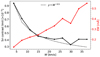 |
Fig. 7 5σ detection limit of the He I airglow emission as a function of the line width of the potential signal using three nights of observationsof τ Boo b (solid black line), and corresponding equivalent widths of the detection limit (solid red curve). The dashed line represents the scaled relation of W−1∕2 that is expected for pure Gaussian white noise. |
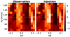 |
Fig. 8 Signal-to-noise ratio map for a grid of planetary orbits with different semiamplitude KP and phase offset Δϕ. There is no salient signal in the observations (left panel). An injected signal at KP = 110 km s−1 and Δϕ = 0 is clearly recovered (right panel). |
5.2 Validation of signal recovery
Prior knowledge of the planetary orbit was used to mask the trail in the spectral series to avoid self-subtraction of the potential signal (see Sect. 4.1). In order to assess the effect of this procedure on the final result, we repeated the whole analysis by adopting a grid of planetary orbits with different semiamplitude KP and phase offset Δϕ when we applied the mask. In Fig. 8 we map the S/N of the residuals at 10 830.3 Å in the planetary rest frame for each hypotheticalorbit in the grid. As a comparison, we produce a similar map when an artificial planetary signal with a strength of 3.3 × 10⁻⁴ and a width of 30 km s−1 was injected, which is recovered at KP = 110 km s−1 and Δϕ = 0 in Fig. 8, also without prior knowledge of the planetary orbit.
6 Discussion
6.1 Detectability of He emission
Using three nights of observations (~6.5 h of integration) on τ Boo b with CARMENES, we reached a contrast limit of 4 × 10⁻⁴ for a planetary He I emission with a boxcar profile with a width >20 km s−1. However, following Eq. (3), the estimated amplitude of the He I emission is typically ≤ 10−4. At this stage, no detection is expected with these observations.
We note that we made several assumptions for simplicity. First, we assumed that the atmosphere extends significantly beyond the planet radius, and the He I cloud was considered to be optically thin. The stellar radiation was assumed to be absorbed uniformly inthe cloud and reemitted isotropically. In addition, Eq. (3) assumes that the energy is conserved at the particular wavelength 10 830 Å, meaning that we only take into account the transition between the helium 23 S and 23 P states.
In practice, the flux ratio can deviate from this simplified model in the following ways. (a) The flux emission of the cloud can be higher than our estimate when the extent of the exosphere is even larger than the stellar disk, in which case the measured fabs in the transmission spectrum is lower than the actual absorption level of the entire cloud. (b) Analysis of the line ratio of He I triplet detected in transmission observations suggests that the planetary signal might also originate from an optically thick part of the atmosphere, especially for Jupiter-mass planets such as HD 189733b and HD 209458b, where the He I absorption feature traces compact atmospheres with an extent of only a fraction of planetary radii (Salz et al. 2018; Lampón et al. 2020). If the cloud is not optically thin or the He I atmosphere is not significantly larger with respect to the planet, the reradiation is not isotropically emitted from the cloud in 4π but with preferential directions, as an analogy to scattered light. In this case, the emission flux at the full phase (i.e., when the illuminated hemisphere is totally in view) is higher than the value in Eq. (3), but it also needs to be scaled with the phase function Φα at different orbital phases (where we observe different portions of the illuminated hemisphere). (c) If the He I cloud is not optically thin, the planetary thermal emission passing through the cloud can be absorbed along the line of sight, which cancels out a portion of the airglow emission. To evaluate this effect, we compared the absorbed thermal emission to the airglow emission flux as follows. Assuming the planet emits as a blackbody with an equilibrium temperature of Tp, we can calculate the planetary thermal emission flux in contrast to the stellar flux at 10 830 Å. Taking τ Boo system as an example, the flux contrast is  . To the optically thick limit, where all thermal emission is absorbed by the He I cloud, it counterbalances ~25% of the airglow emission. Even in the extreme optically thick case, the helium is consequently expected to be seen in emission. (d) The emission level of He I 10 830 Å is determined by the population of helium in the 23 P state and by the rates of the stimulated and spontaneous decay of 23P state. Studying this requires detailed accounts and comparisons of other depopulating processes, including photoionization from the 23 P state, collisions of electrons and H-atoms, and radiative excitation to 23D state (D3 line). Previous models of helium atmospheres, such as Oklopčić & Hirata (2018) and Lampón et al. (2020), neglected transitions related to 23P state because the metastable 23S state population is not significantly affected by these processes as an atom in the 23 P state just decays back to 23 S state (Oklopčić & Hirata 2018). This indicates that the 23P to 23S decay is the main way of depopulating the 23P state. We therefore argue that the level of absorption and the airglow emission at 10 830 Å are connected.
In addition to the amplitude of the He I emission, the velocity profile is rather uncertain. Current detections suggest that the He I excess absorption spans a wide range of line widths. For instance, Saturn- or Neptune-mass planets such as WASP-69b and HAT-P-11b (Allart et al. 2018; Nortmann et al. 2018) are reported to have broad absorption features (up to ~30 km s−1), while Jupiter-mass planets such as HD 209485b (Alonso-Floriano et al. 2019) show a more narrow signature of ~10 km s−1, implying a lower rate of atmospheric escape and mass loss. The line profile depends on the physical and hydrodynamic properties such as the kinematic temperature of the exosphere and the atmospheric escape, which are not well understood (Salz et al. 2016). Considering the diverse nature of planetary atmospheres, we therefore recommend to explore a variety of line widths and line positions in data analysis.
6.2 Future prospects
6.2.1 Observation design
Based on our data analysis, we find several aspects that should be taken into account when future observations to search for He I airglow emission are designed. First, the observations should avoid blending the planetary helium signal with strong telluric absorption lines (such as during our night 2 observations). In this situation, a large portion of the emission signal is removed along with the telluric correction. Even if the signal is preserved with other methods, strong telluric features cannot be corrected for perfectly, which introduces artifacts around the helium signal. Furthermore, the S/N of observations at the core of strong telluric absorption lines is significantly lower than in the continuum. Hence, the potential signal falling in such region is more difficult to detect. It is therefore desirable to take the relative position between the planetary and telluric lines into account and to select the proper time for observations according to the barycentric Earth radial velocity and the planetary radial velocity.
The stellar activity is yet another factor to consider in data analysis because the stellar He I line as a chromospheric diagnostic may undergo temporal variation during observations. For an active star like τ Boo, this is likely to happen and introduce additional noise. Cauley et al. (2018), Salz et al. (2018), and Guilluy et al. (2020) evaluated the effect of stellar activity on probing the planetary helium atmosphere in transmission. However, unlike transit observations, additional noise related to stellar activity is not expected to significantly affect measurements of emission signals from a planet because there is always a radial velocity offset between the star and planet when emission is probed. Only when the radial velocity difference is small (i.e., during transit and secondary eclipse) can stellar activity contribute to noise at the planetary rest frame and result in pseudo-signals. In terms of detecting airglow emission, the likely consequence of the variability of stellar He I line is that systematic noise structure is introduced nearby the planetary signal in the temporal-combined residual spectrum, instead of affecting the level of planetary signal. Consequently, for highly active stars, there needs to be sufficient difference between the planet and stellar radial velocity, which depends on the orbital phase, during observations.
In terms of target selection, we performed the case study on τ Boo because the star is significantly brighter than other known hot-Jupiter systems, enabling high S/N observations. In addition, itshigh level of stellar activity likely results in an extended planetary atmosphere in which the He I 23 S is populated. As shown in Fig. 9, when we account for the stellar brightness and the airglow emission signal estimated using Eq. (3), τ Boo b falls closest to our detection limit (denoted by the dashed line) among other potential targets. In calculating the emission signal, as we have no measurements of the He I absorption by the nontransiting τ Boo b, we assumed an absorption level of 1%, which brings about some uncertainty, however. τ Boo as an F-type star may also have high levels of mid-UV radiation that can depopulate the helium triplet states, leading to a weaker signal. It remains unclear to what extent these various factors contribute to the He I signal as a whole. In addition, the planet mass is significantly higher than that of most hot Jupiters, which increases the surface gravity and might make atmosphericescape more difficult (Salz et al. 2016). A more secure choice is to investigate targets whose He I absorption has been measured with transmission spectroscopy (denoted with red dots in Fig. 9), so that the emission amplitude is known beforehand. Another benefit of targeting a transit planet is that we would be able to obtain the stellar spectrum without any contribution from the planet during secondary eclipse. Using this as a reference spectrum, we would be able to avoid self-subtracting the planetary signal in analysis, which is particularly important for broad signatures. Furthermore, as discussed in Sect. 6.1, the airglow emission signal is partially counterbalanced by absorption of planet thermal emission through the He I cloud when it is compact. Consequently, planets with puffy and optically thin He I clouds are better targets for this purpose.
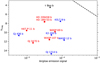 |
Fig. 9 V magnitude of host stars plotted against the airglow emission signal estimated using Eq. (3) for exoplanets with He I absorption detections (red dots) or upper limits (blue triangles). The black star represents the estimated signal of τ Boo b assuming a typical absorption level of 1%. The dashed black line shows the detection limit of our analysis. |
6.2.2 Search with VLT/CRIRES+ and E-ELT/HIRES
CRIRES+ is an upgrade of the cryogenic high-resolution infrared echelle spectrograph (CRIRES) located at the focus of UT1 of the Very Large Telescope (VLT), providing a spectral resolving power of 100 000 (Follert et al. 2014). When we simply scale the expected S/N for observations with CRIRES+ by the larger telescope diameter of the 8.2 m VLT compared to the 3.5 m Calar Alto Telescope, also considering that the throughput of CRIRES+ may be a factor of 1.5 lower than that of CARMENES while the observing condition at VLT site is generally better, we expect to go a factor ~2 deeper in the same observing time. Accordingly, we expect to reach a detection limit of 2 × 10⁻⁴ for a broad He I emission given the same amount of integration (~6.5 h). Taking τ Boo b as an example, following Eq. (3), we estimate the amplitude of the emission to be ~ 5 × 10⁻⁵ assuming a typical “transit” absorption level of 1%. This means that a 3σ detection of He I airglow emission could be obtained in about five observation nights. Although probing He I emission is demanding using the current generation of telescopes, it is promising with the High Resolution Spectrograph (HIRES) at ESO’s forthcoming Extremely Large Telescope (E-ELT; Marconi et al. 2016). The significantly larger diameter of the 39m E-ELT means that the 5σ detection of He I airglow emission could be achieved with ~3 h of integration. Of course there is a large uncertainty in the expected level of emission, which can at least partly be mitigated by choosing a transiting planet.
7 Conclusions
We explored the possibility of probing He I emission at 10 830 Å in the extended atmospheres of hot Jupiters, the amplitude of which is estimated based on the He I absorption level as observed during transit. We searched for this emission from τ Boo b using CARMENES spectra. We corrected for the telluric and stellar features nearby the expected He I signal and combined multiple nights of observations. Given our estimate of the contrast of ≤ 10−4, the 6.5-h data combined are not sufficient to place meaningful constraints on the He I emission from the planet. The detection limit that we derive from our analysis is 4 × 10⁻⁴ for a broad emission signal with a width of >20 km s−1. While we donot reach the required contrast with the current CARMENES data, the He I airglow emission from hot Jupiters is still promising to probe with future instruments.
Acknowledgements
We thank the referee and editor for comments which helped improving the quality of the paper. Y.Z., I.S., F.A., and P.M. acknowledge funding from the European Research Council (ERC) under the European Union’s Horizon 2020 research and innovation program under grant agreement No 694513. P.M. acknowledges support from the European Research Council under the European Union’s Horizon 2020 research and innovation program under grant agreement No. 832428. M.B. acknowledges support from the UK Science and Technology Facilities Council (STFC) research grant ST/S000631/1. A.W. acknowledges the financial support of the SNSF by grant number P2GEP2-178191 and P400P2-186765.
Appendix A Derivation of the helium emission strength with radiative transfer
During transit, the stellar flux  decreases by
 as a result of the absorption by helium atoms at 23S state. The absorption depth Tλ measured by transmission spectroscopy is
 (A.1)
(A.1)
where τc is the optical depth of the He I cloud around the planet, and the structure of the cloud is neglected.
A.1 Optically thick He I clouds
For optically thick clouds, τc ≫ 1, Eq. (A.1) becomes
 (A.2)
(A.2)
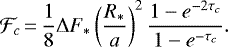
The emission flux from the cloud can be approximated as isotropic scattering with an albedo of 1, resulting in a factor of 2/3 of the received flux (Seager 2010),
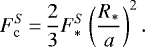 (A.3)
(A.3)
SubstitutingEqs. (2) and (A.2) into Eq. (A.3), we obtain
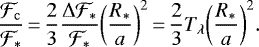 (A.4)
(A.4)
A.2 Optically thin He I clouds
For optically thin cases, we consider the simplified 1D plane-parallel equation of radiative transfer,
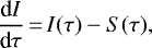 (A.5)
(A.5)
where Iν is the spectral radiance, S is the source function, and τ is the extinction optical depth, which increases toward the interior of the cloud (i.e., the optical depth at the interior is τc and that at the surface is 0).
The source function is approximated as
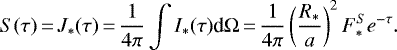 (A.6)
(A.6)
Hence, the solution for the equation of radiative transfer can be composed as
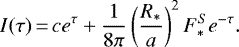 (A.7)
(A.7)
Using the boundary condition I(τc) = 0, we determine the integral constant c, which simplifies the solution as
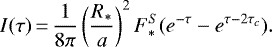 (A.8)
(A.8)
Then the emergent radiance from the cloud Ic is
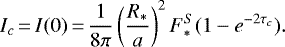 (A.9)
(A.9)
The observed flux of the cloud is
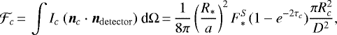 (A.10)
where nc and n detector represent the unit vectors along the intensity of the cloud and the normal direction of the detector surface, respectively. Because the targets are far away, we can safely assume nc ⋅ndetector = 1 in Eq. (A.10).
Substituting 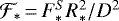 and Eqs. (A.1) into (A.10), we have
 (A.11)
At the optically thin limit (τc ≪ 1), Eq. (A.11) reduces to
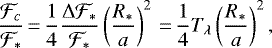 (A.12)
which agrees with Eq. (3).
References
- Allart, R., Bourrier, V., Lovis, C., et al. 2018, Science, 362, 1384 [Google Scholar]
- Allart, R., Bourrier, V., Lovis, C., et al. 2019, A&A, 623, A58 [NASA ADS] [CrossRef] [EDP Sciences] [Google Scholar]
- Alonso-Floriano, F. J., Snellen, I. A. G., Czesla, S., et al. 2019, A&A, 629, A110 [NASA ADS] [CrossRef] [EDP Sciences] [Google Scholar]
- Andretta, V., Giampapa, M. S., Covino, E., Reiners, A., & Beeck, B. 2017, ApJ, 839, 97 [Google Scholar]
- Borsa, F., Scandariato, G., Rainer, M., et al. 2015, A&A, 578, A64 [NASA ADS] [CrossRef] [EDP Sciences] [Google Scholar]
- Bourrier, V., Lecavelier des Etangs, A., Ehrenreich, D., et al. 2018, A&A, 620, A147 [NASA ADS] [CrossRef] [EDP Sciences] [Google Scholar]
- Brogi, M., Snellen, I. A. G., de Kok, R. J., et al. 2012, Nature, 486, 502 [Google Scholar]
- Butler, R. P., Marcy, G. W., Williams, E., Hauser, H., & Shirts, P. 1997, ApJ, 474, L115 [Google Scholar]
- Caballero, J. A., Guàrdia, J., López del Fresno, M., et al. 2016, SPIE Conf. Ser., 9910, 99100E [Google Scholar]
- Cauley, P. W., Kuckein, C., Redfield, S., et al. 2018, AJ, 156, 189 [Google Scholar]
- Crossfield, I. J. M., Barman, T., Hansen, B., & Frewen, S. 2019, Res. Notes Am. Astron. Soc., 3, 24 [Google Scholar]
- Ehrenreich, D., Bourrier, V., Wheatley, P. J., et al. 2015, Nature, 522, 459 [Google Scholar]
- Follert, R., Dorn, R. J., Oliva, E., et al. 2014, SPIE Conf. Ser., 9147, 914719 [Google Scholar]
- Gaia Collaboration (Brown, A. G. A., et al.) 2018, A&A, 616, A1 [NASA ADS] [CrossRef] [EDP Sciences] [Google Scholar]
- Gaidos, E., Hirano, T., Mann, A. W., et al. 2020, MNRAS, 495, 650 [Google Scholar]
- Guilluy, G., Andretta, V., Borsa, F., et al. 2020, A&A, 639, A49 [EDP Sciences] [Google Scholar]
- Hirano, T., Krishnamurthy, V., Gaidos, E., et al. 2020, ApJ, 899, L13 [Google Scholar]
- Huensch, M., Schmitt, J. H. M. M., & Voges, W. 1998, A&AS, 132, 155 [NASA ADS] [CrossRef] [EDP Sciences] [Google Scholar]
- Justesen, A. B., & Albrecht, S. 2019, A&A, 625, A59 [EDP Sciences] [Google Scholar]
- Kirk, J., Alam, M. K., López-Morales, M., & Zeng, L. 2020, AJ, 159, 115 [Google Scholar]
- Kreidberg, L., & Oklopčić, A. 2018, Res. Notes AAS, 2, 44 [Google Scholar]
- Kulow, J. R., France, K., Linsky, J., & Loyd, R. O. P. 2014, ApJ, 786, 132 [Google Scholar]
- Lampón, M., López-Puertas, M., Lara, L. M., et al. 2020, A&A, 636, A13 [CrossRef] [EDP Sciences] [Google Scholar]
- Lockwood, A. C., Johnson, J. A., Bender, C. F., et al. 2014, ApJ, 783, L29 [Google Scholar]
- Mansfield, M., Bean, J. L., Oklopčić, A., et al. 2018, ApJ, 868, L34 [Google Scholar]
- Marconi, A., Di Marcantonio, P., D’Odorico, V., et al. 2016, SPIE Conf. Ser., 9908, 990823 [Google Scholar]
- Ninan, J. P., Stefansson, G., Mahadevan, S., et al. 2020, ApJ, 894, 97 [Google Scholar]
- Nortmann, L., Pallé, E., Salz, M., et al. 2018, Science, 362, 1388 [Google Scholar]
- Oklopčić, A. 2019, ApJ, 881, 133 [Google Scholar]
- Oklopčić, A., & Hirata, C. M. 2018, ApJ, 855, L11 [Google Scholar]
- Owen, J. E. 2019, Ann. Rev. Earth Planet. Sci., 47, 67 [Google Scholar]
- Palle, E., Nortmann, L., Casasayas-Barris, N., et al. 2020, A&A, 638, A61 [EDP Sciences] [Google Scholar]
- Quirrenbach, A., Amado, P. J., Caballero, J. A., et al. 2016, SPIE Conf. Ser., 9908, 990812 [Google Scholar]
- Salz, M., Czesla, S., Schneider, P. C., & Schmitt, J. H. M. M. 2016, A&A, 586, A75 [NASA ADS] [CrossRef] [EDP Sciences] [Google Scholar]
- Salz, M., Czesla, S., Schneider, P. C., et al. 2018, A&A, 620, A97 [NASA ADS] [CrossRef] [EDP Sciences] [Google Scholar]
- Sanz-Forcada, J., Micela, G., Ribas, I., et al. 2011, A&A, 532, A6 [NASA ADS] [CrossRef] [EDP Sciences] [Google Scholar]
- Seager, S. 2010, Exoplanet Atmospheres: Physical Processes (Princeton: Princeton University Press) [Google Scholar]
- Seager, S., & Sasselov, D. D. 2000, ApJ, 537, 916 [Google Scholar]
- Spake, J. J., Sing, D. K., Evans, T. M., et al. 2018, Nature, 557, 68 [Google Scholar]
- Takeda, G., Ford, E. B., Sills, A., et al. 2007, ApJS, 168, 297 [Google Scholar]
- Vidal-Madjar, A., Lecavelier des Etangs, A., Désert, J. M., et al. 2003, Nature, 422, 143 [Google Scholar]
- Wright, J. T., Marcy, G. W., Butler, R. P., & Vogt, S. S. 2004, ApJS, 152, 261 [NASA ADS] [CrossRef] [Google Scholar]
All Tables
All Figures
|
Fig. 1 Illustration of He I emission from an exosphere of a close-in planet. The gray disk represents the extended atmosphere around such a planet. He I absorption is observed during transit, while airglow emission can be probed at other orbital phases. |
| In the text | |
|
Fig. 2 Variation in airmass (upper panel), relative humidity (mid panel), S/N (lower panel) and variation around the mean of thestellar He I line (bottom panel) during observations in the different nights. The S/N of each spectrum is defined as the average signal-to-noise ratio of the continuum near the He I 10 830 Å line. |
| In the text | |
|
Fig. 3 Illustration of the data reduction steps we applied to the spectral series taken on night 4. Each row in the matrix represents one spectrum, and the y-axis corresponds to time. As detailed in Sect. 4.1, the steps include (a) normalization of the continuum, (b) correction for stellar lines in each spectrum using an empirical model, and (c) removal of telluric contamination by correcting the temporal variation of the flux in telluric lines using a column-by-column linear regression. The trail of an artificially injected planetary helium line (with a magnitude of 0.3% and a width of 11 km s−1) is visible as a slanted white band near 10 830 Å that shifts in time as a result of the change in the radial component of the orbital velocity of the planet. |
| In the text | |
|
Fig. 4 Residual spectral series from nights 1 to 5. The y-axis represents the time or orbital phase. The residuals are binned to 0.006 in phase for clarity. The slanted dashed lines in red trace the expected planetary helium line. The dotted lines in blue denote the positions of the stellar He I triplet. The shaded region in night 2 contains the telluric H2O absorption and OH emission line, which overlap the expected planetary helium line. |
| In the text | |
|
Fig. 5 Upper panel: average profile of the stellar helium line in each night. Lower panel: difference of each profile with respect to the mean. The deep absorption line at 10 832.2 Å in night 2 (blue curve) is a telluric H2O line. The small peaks on top of the helium line in night 1 and 5 are caused by sky OH emission. |
| In the text | |
|
Fig. 6 Combined (three nights) residual spectra in the planetary rest frame centered at the 10 830 Å He I line. In the three panels, the solid black line indicates the residual spectra, boxcar-smoothed by 3.7 km s−1 (top), 14.9 km s−1 (middle), and 29.8 km s−1 (bottom). The dotted curves show an artificially injected signal at an S/N of 5, and the solid red curve shows the difference between the injectedand original data. The values are scaled by the standard deviation of the observed residuals so that the y-axis represents the S/N. |
| In the text | |
|
Fig. 7 5σ detection limit of the He I airglow emission as a function of the line width of the potential signal using three nights of observationsof τ Boo b (solid black line), and corresponding equivalent widths of the detection limit (solid red curve). The dashed line represents the scaled relation of W−1∕2 that is expected for pure Gaussian white noise. |
| In the text | |
|
Fig. 8 Signal-to-noise ratio map for a grid of planetary orbits with different semiamplitude KP and phase offset Δϕ. There is no salient signal in the observations (left panel). An injected signal at KP = 110 km s−1 and Δϕ = 0 is clearly recovered (right panel). |
| In the text | |
|
Fig. 9 V magnitude of host stars plotted against the airglow emission signal estimated using Eq. (3) for exoplanets with He I absorption detections (red dots) or upper limits (blue triangles). The black star represents the estimated signal of τ Boo b assuming a typical absorption level of 1%. The dashed black line shows the detection limit of our analysis. |
| In the text | |
Current usage metrics show cumulative count of Article Views (full-text article views including HTML views, PDF and ePub downloads, according to the available data) and Abstracts Views on Vision4Press platform.
Data correspond to usage on the plateform after 2015. The current usage metrics is available 48-96 hours after online publication and is updated daily on week days.
Initial download of the metrics may take a while.