| Issue |
A&A
Volume 641, September 2020
|
|
|---|---|---|
| Article Number | A31 | |
| Number of page(s) | 30 | |
| Section | Extragalactic astronomy | |
| DOI | https://doi.org/10.1051/0004-6361/202038184 | |
| Published online | 01 September 2020 | |
From spirals to lenticulars: Evidence from the rotation curves and mass models of three early-type galaxies
1
ESO, Karl-Schwarschild-Strasse 2, 85748 Garching bei München, Germany
e-mail: This email address is being protected from spambots. You need JavaScript enabled to view it.
2
Department of Physics, Harvard University, 17 Oxford Street, Cambridge, MA 02138, USA
3
School of Physics and Astronomy, Cardiff University, Queens Buildings, The Parade, Cardiff CF24 3AA, UK
Received:
16
April
2020
Accepted:
16
June
2020
Abstract
Rotation curves have traditionally been difficult to trace for early-type galaxies (ETGs) because they often lack a high-density disk of cold gas as in late-type galaxies (LTGs). In this work, we derive rotation curves for three lenticular galaxies from the ATLAS3D survey, combining CO data in the inner parts with deep HI data in the outer regions, extending out to 10−20 effective radii. We also use Spitzer photometry at 3.6 μm to decompose the rotation curves into the contributions of baryons and dark matter (DM). We find that (1) the rotation-curve shapes of these ETGs are similar to those of LTGs of a similar mass and surface brightness; (2) the dynamically-inferred stellar mass-to-light ratios are small for quiescent ETGs but similar to those of star-forming LTGs; (3) the DM halos follow the same scaling relations with galaxy luminosity as those of LTGs; and (4) one galaxy (NGC 3626) is poorly fit by cuspy DM profiles, suggesting that DM cores may exist in high-mass galaxies too. Our results indicate that these lenticular galaxies have recently transitioned from LTGs to ETGs without altering their DM halo structure (e.g., via a major merger), and they could be faded spirals. We also confirm that ETGs follow the same radial acceleration relation as LTGs, reinforcing the notion that this is a universal law for all galaxy types.
Key words: galaxies: elliptical and lenticular, cD / galaxies: evolution / dark matter / galaxies: spiral / galaxies: kinematics and dynamics
© ESO 2020
1. Introduction
Extended rotation curves and mass models have been derived for hundreds of late-type galaxies (LTGs: spirals and irregulars), but only for a few early-type galaxies (ETGs: ellipticals and lenticulars) because they often lack high-density HI disks (e.g., Lelli et al. 2016). Traditionally, dynamical studies of ETGs have relied on different kinematic tracers. One approach is to combine stellar kinematics in the inner parts (e.g., Cappellari 2016) with discrete tracers such as planetary nebulae and globular clusters in the outer regions (e.g., Forbes et al. 2016). Alternatively, strong lensing (e.g., Gerhard 2013) and X-ray halos (e.g., Buote & Humphrey 2012) have also been used to trace the mass distribution of ETGs. These methods allowed one to study the dark matter (DM) content of ETGs, but a direct comparison with LTGs has been highly nontrivial since different methods require different assumptions (e.g., Janz et al. 2016; Lelli et al. 2017). For example, studies of stellar kinematics and discrete tracers rely on assumptions about the orbital anisotropy and the tracer population, studies of X-ray halos hold under the assumption of hydrostatic equilibrium, while strong lensing studies may depend on the lensing model and are generally limited to the inner galactic radii.
On the other hand, cold gas (both atomic and molecular) is a more straightforward tracer of the gravitational potential for a number of reasons: (1) the cold gas forms thin rotating disks in which the pressure support is negligible, so the rotation velocity directly traces the circular velocity of a test particle in the given gravitational potential; (2) noncircular motions are generally small, contrary to the ionized gas traced by Hα and [OIII] lines; and (3) the atomic gas, if present, can extend to large radii, well beyond the bright stellar component. However, analyzing the gas kinematics of ETGs as it is done for LTGs has long been challenging due to the low surface brightness of the gas emission (e.g., Weijmans et al. 2008; Struve et al. 2010). Deep, interferometric radio surveys have been able to detect and spatially resolve the HI emission in ETGs in group and field environments (Serra et al. 2012), showing that the atomic gas often forms regularly rotating disks extending out to large radii. Moreover, deep CO observations have revealed that many ETGs host inner disks of molecular gas (Alatalo et al. 2013; Davis et al. 2013). These key observational advances allow us to study the cold gas kinematics in ETGs in detail, providing new insights into the DM halos of different galaxy types.
In this work, we derive rotation curves and mass models of three ETGs from the ATLAS3D survey (Cappellari et al. 2011a): NGC 2824, NGC 3626, and UGC 6176. These are the only three galaxies in the ATLAS3D sample that have both an inner CO disk and an outer HI disk. We combine CO and HI kinematics to determine accurate rotation curves in a uniform way over the entire extent of the gaseous body. Some of the known properties of the galaxies are summarized in Table 1. They are morphologically classified as lenticulars (S0) and identified as “fast rotators” based on their observed stellar kinematics (Cappellari et al. 2011a). In particular, NGC 3626 is a well-studied object since it has a stellar component that counter-rotates with respect to the gaseous disk (Ciri et al. 1995; Jore et al. 1996; Haynes et al. 2000; Sil’chenko et al. 2010; Mazzei et al. 2014). NGC 3626 also has a companion galaxy (UGC 6341, see Fig. 1) with significant HI emission (Serra et al. 2012), which we do not study here.
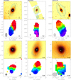 |
Fig. 1. Moment maps for NGC 2824 (left), NGC 3626 (middle), and UGC 6176 (right). The top section shows the HI data, while the bottom section shows the CO data. In each section, the top row shows the Spitzer image at 3.6 μm overlaid with the gas intensity maps, while the bottom row shows the velocity field. The box in the HI velocity field depicts the size of the CO frame. The cross corresponds to the galaxy center; the dashed line indicates the kinematic major axis; the physical scale is illustrated in the bottom-right corner; the beam shape is shown in the bottom-left corner. The HI and CO density contours are multiples of the pseudo-3σ value (0.5, 1, 2, 4, ...) where 3σmap is given in Table 2. |
Galaxy sample.
2. HI and CO moment maps
We analyze public HI and CO cubes from the Atlas3D website (Serra et al. 2012; Alatalo et al. 2013). For NGC 2824, we use a deeper HI cube that was kindly provided to us by Dr. Paolo Serra. The cube properties are summarized in Table 2. We perform our analysis using the Groningen imaging processing system (GIPSY, van der Hulst et al. 1992) and 3DBarolo (3D-Based Analysis of Rotating Object via Line Observations, Di Teodoro & Fraternali 2015). We create masks that identify regions of gas emission using the “smooth and search” algorithm of 3DBarolo with the parameter threshVelocity set to 1 and minPix set to the beam size of each cube. We apply these masks to the full-resolution cubes to create intensity maps (moment-zero), summing all channels that contain line emission, and velocity maps (moment-one), estimating an intensity-weighted mean velocity. Velocity dispersion maps (moment-two) have little physical meaning since the line broadening is largely driven by beam-smearing effects rather than representing the true, intrinsic velocity dispersion of the gas. The average root-mean-square noise in the cubes is determined using channels that are free of line emission. In the intensity maps, a pseudo-3σ contour is estimated using the formulae from Verheijen & Sancisi (2001) and Lelli et al. (2014), which account for the different number of summed channels at each spatial pixel and for the channel dependencies.
Properties of the analyzed datacubes.
Figure 1 shows the intensity maps superimposed on the Spitzer [3.6] images (top rows) and the velocity maps (bottom rows). For all three galaxies, the HI distribution is more extended than the stellar body, while the CO distribution is concentrated near the galactic center. Both HI and CO velocity fields display regular rotation with no clear signs of strong noncircular motions. This is also evinced by position-velocity (PV) diagrams extracted along the kinematic major axis of the disk, which are shown in Fig. 2. The morphological position angle (PA) from the intensity maps agrees with the kinematic PA from the velocity maps. It also agrees with the orientation of the stellar bodies for NGC 2824 and UGC 6176. For NGC 3626, instead, the PA suggested by the elongation of the stellar disk differs from the average HI major axis, pointing to a warped gas disk.
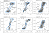 |
Fig. 2. Major-axis PV diagrams from the observed HI cube (top row) and the CO one (bottom row), overlaid with the projected rotation curve (white squares) and model PV diagrams (blue contour corresponding to 1.5σ from Table 2). |
3. Derivation of rotation curves
We derive rotation curves by fitting the velocity fields with a tilted-ring model to obtain initial estimates, which are subsequently refined by building kinematic 3D disk models (e.g., Lelli et al. 2012a, 2012b). We also verified our results using the software 3DBarolo (Di Teodoro & Fraternali 2015), which directly fits the 3D cube bypassing the 2D velocity maps.
In the tilted-ring fit, each ring is described by six free parameters: center (x0, y0), systemic velocity (vsys), position angle (PA), inclination (i), and rotation velocity (vrot). The width of the rings is chosen to be either equal to the width of the beam major axis, or  if the beam is strongly elongated and not aligned with the PA of the galaxy. Here, bmaj and bmin are the major and minor axes of the beam, respectively. The number of rings is determined such that the major axis of the galaxy is fully covered. The pixels in the velocity maps are weighted using a cosine function to give more weight to points close to the major axis, which provide most information regarding the rotation velocity. We simultaneously fit both halves of the galaxy, neglecting possible asymmetries between the different sides. For NGC 3626, however, the CO data do not cover the full gas emission at approaching velocities due to the limited bandwidth of the observations, so we fit only the receding side.
We perform a series of iterations using the GIPSY task rotcur (Begeman 1987). In the first iteration all the parameters are left free, while in the second iteration we fix x0, y0, and vsys using the mean values across the rings. The centers and systemic velocities from the CO and HI data are consistent with each other, as well as with optical determinations from the Nasa Extragalactic Database. In the next two iterations, the PA and inclination are fixed in arbitrary order. We have checked that the order does not change the resulting rotation curve within the errors. For NGC 2824 and UGC 6176, the CO and HI disks show no strong indications of warps, so i and PA are kept constant with radius. For both galaxies, however, the inner CO inclination significantly differ from the outer HI inclination. For NGC 3626, we model an HI warp by varying both PA and i with radius. The last run of rotcur is performed leaving only vrot as a free parameter.
To check the resulting rotation curves and correct for beam smearing effects, we construct model cubes using the rotcur results and the observed gas density profiles as inputs. We derive azimuthally-averaged HI and CO surface brightness profiles using the GIPSY task ellint, adopting the best-fit geometric parameters. The CO surface brightnesses are converted into H2 surface densities adopting the Milky-Way conversion factor XCO = 2 × 1020 cm−2 (K km s−1)−1 (Bolatto et al. 2013). We create model cubes with the GIPSY task galmod for the HI data and a custom-built task for the CO data. Since the latter task does no automatic conversion from H2 surface density to CO surface brightness, we renormalize the total flux of the CO model to be equal to the observed flux. We assume that the gas disk has a velocity dispersion of 10 km s−1 and a thickness of 100 pc.
We compare PV diagrams and channel maps from the model cubes with the observed ones. A disagreement between models and observations indicates that the input density profiles and/or rotation curves are affected by beam smearing. Beam smearing tends to flatten the surface density profile and cause an underestimation of the rotation velocity, especially in the innermost regions. We manually adjust individual points in the inner parts of the rotation curves and/or density profiles to minimize the residuals. In some cases, the PA and inclination angle are also manually adjusted by a few degrees to find the best compromise between the kinematic estimates from rotcur and the observed intensity maps. The best-fit 3D models are illustrated in Fig. 2 and presented in a more extensive way in Appendix A. The adopted geometric parameters are summarized in Tables 3 and 4 for the warp model of NGC 3626. The uncertainties are estimated by running 3DBarolo with all the parameters fixed to the final value and only one parameter of interest left free. The final geometric parameters and rotation curves are shown in Fig. 3.
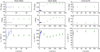 |
Fig. 3. Position angle (top), inclination (middle), and final rotation curves (bottom) from HI (green points) and CO (blue triangles) observations. Open circles show omitted points in the combined rotation curves due to the overlap of CO and HI data. |
Geometric parameters of CO and HI disks.
Warp model for NGC 3626.
In general, 3DBarolo returns similar rotation curves as our manual procedure with some exceptions. For NGC 2824, the CO data have too low spatial resolutions and signal-to-noise ratio to ensure a good 3DBarolo fit, while the HI data shows a strong absorption feature at small radii that 3DBarolo cannot model. For NGC 3626, the missing CO data at approaching velocities cannot be automatically modeled by 3DBarolo, whereas our manual procedure can take this shortcoming into account by focusing on the receding portion of the PV diagram. For these reasons, we prefer our manual procedure with respect to fully automatic fits with 3DBarolo.
We combine the CO and HI rotation curves into a single, optimal rotation curve. At radii where rotation velocities are available from both tracers, we favor the CO data since beam-smearing effects are less severe due to their higher spatial resolution. For NGC 2824 and NGC 3626, the combined rotation curves rise steeply in the central parts, decline at intermediate radii, and flattens in the outer regions. Similar rotation curves are often observed in massive spiral galaxies (Casertano & van Gorkom 1991; Noordermeer et al. 2007). For UGC 6176, the rotation curve is almost perfectly flat, similarly to spiral galaxies of lower masses (e.g., Begeman 1987). The shapes of the rotation curves are further discussed in Sect. 6.
4. Mass models
We derive detailed mass models using Spitzer 3.6 μm images to estimate the stellar gravitational field, together with HI and CO maps to estimate the gas gravitational field (Fig. 1). In Sect. 5, we use these mass models and the observed rotation curves to study the DM halos of our three lenticular galaxies.
4.1. Stellar and gaseous contributions
The SPARC database (Spitzer Photometry and Accurate Rotation Curves, Lelli et al. 2016) provides [3.6] luminosity profiles and nonparametric bulge-disk decompositions for several ETGs in Atlas3D including our three S0s (see Lelli et al. 2017). Given the intrinsic ambiguity of bulge-disk decompositions for lenticular galaxies, we explored different decompositions’ scheme to estimate their impact on the final mass models. After several trials, we decided to use a single, disk-like component for both NGC 2824 and NGC 3626 because the bulge contribution is small and uncertain. This is a conservative choice that avoids adding unnecessary free parameters to the mass model. All the observed features in the surface brightness profiles are preserved in calculating the stellar gravitational contribution, including the inner light concentrations. For NGC 2824 and NGC 3626, we simply assume that these light concentrations lie in a flattened structure with a similar mass-to-light ratio as the stellar disk, as it may be the case for a pseudo-bulge (e.g., Kormendy & Freeman 2004). For UGC 6176, we use the same bulge-disk decomposition as in Lelli et al. (2017).
We calculate the gravitational contribution of each component using the GIPSY task rotmod. We assume a spherical bulge (when present) and thick disks with a vertical exponential profile. The scale-heights of the HI and CO disks are set to 100 pc, while that of the stellar disk (hz) is assumed to correlate with the exponential scale-length (hR) as  (Bershady et al. 2010). This relation has been derived for edge-on spiral galaxies and may be potentially inappropriate for lenticular galaxies (see, e.g., de Grijs 1998). Luckily, the 3D geometry of baryons has a minor effect on the final mass models: the maximum variation in the peak circular velocities is about 20% for axial ratios between zero (razor-thin disk) and one (sphere); see, for example, Fig. 3 in Noordermeer (2008). This effect is smaller than the current uncertainties in the stellar mass-to-light ratios from stellar population models (e.g., Schombert et al. 2019). Having computed the gravitational field of the individual components in the disk mid-plane, the baryonic rotation curve reads
![Mathematical equation: $$ \begin{aligned} { v}^2_{\mathrm{bar}}(R) = \Upsilon _{\mathrm{d}} { v}^2_{\mathrm{d}}(R) + \Upsilon _{\mathrm{b}} { v}^2_{\mathrm{b}}(R) + 1.33\left[{ v}^2_{\mathrm{HI}}(R) + { v}^2_{\mathrm{H2}}(R)\right], \end{aligned} $$](/articles/aa/full_html/2020/09/aa38184-20/aa38184-20-eq3.gif) (1)
(1)
where vd and vb account for the stellar contribution (disk and bulge, respectively), while vHI and vH2 account for the gas contribution (atomic and molecular, respectively). The molecular contribution is computed assuming the standard conversion factor XCO = 2 × 1020 cm−2 (K km s−1)−1 of the Milky Way. Υ denotes the mass-to-light ratio for the stellar disk and the bulge, indicated by the subscripts d and b, respectively. The 1.33 factor in front of the gaseous components takes the mass contribution of primordial helium into account (Lelli et al. 2016, but see also McGaugh et al. 2020). Table 5 provides the circular velocities and the surface densities of the individual components at the same radii at which rotation velocities are measured.
Rotation curves and mass models for three lenticular galaxies.
4.2. Maximum-disk mass models
The baryonic rotation curve depends on the adopted stellar mass-to-light ratios (Eq. (1)). Here we adjust their values to achieve a maximum-disk fit (van Albada & Sancisi 1986; Starkman et al. 2018), ensuring that the inner part of the observed rotation curve is fully explained by luminous matter. Our fits can be seen in Fig. 4 along with the maximal values of Υb and Υd. Surprisingly, the maximum mass-to-light ratios are relatively small for red and dead ETGs, which are expected to be in the range 0.8−1.0 M⊙/L⊙ (Schombert & McGaugh 2014), but are near the high-end boundary of the expectations for star-forming LTGs (Schombert et al. 2019). This is further discussed in Sect. 6. The baryonic rotation curves do not agree with the observed ones at large radii. This indicates the presence of the DM effect in the galaxies, as we investigate in the next Section.
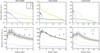 |
Fig. 4. Top panels: surface density profiles for the H2 disk (blue circles), HI disk (green upward triangles), stellar disk (yellow downward triangles), and stellar bulge (red diamonds) when necessary. Open circles indicate that the surface density is extrapolated from an exponential fit. Bottom panels: observed rotation curve (dots with ±1σ error bars) is fit with a maximum-disk mass models (black solid line with ±1σ error band). The baryonic rotation curve is decomposed into the contributions of molecular gas (blue dashed line), atomic gas (green dash-dotted line), stellar disk (yellow solid line), and stellar bulge (red dotted line) when necessary. The maximum mass-to-light ratios are given in the top right corner. |
5. Dark matter halo fits
To model the discrepancy between the observed and baryonic rotation curves at large radii (Fig. 4), we add a DM halo to the mass models. We fit three different halo profiles: NFW (Navarro et al. 1996), Einasto (Einasto 1965), and DC14 (Di Cintio et al. 2014). While the NFW and Einasto profiles are suggested by DM-only cosmological simulations (e.g., Dutton & Macciò 2014), the DC14 profile is derived from hydrodynamical simulations of galaxy formation, and is taking into account the effects of the stellar feedback on the inner DM halo.
Rotation-curve fits with the DC14 profile are described in Katz et al. (2017) and Li et al. (2019, 2020). In short, the shape of the DC14 profile depends on the quantity X = log(M⋆/M200) where M⋆ is the present-day stellar mass and M200 is the halo mass, defined as the enclosed mass at which the halo density equals 200 times the critical density of the Universe. For −4 < X < −2, the DC14 profile is shallower than the NFW profile due to the formation of central DM cores by stellar feedback. For higher and lower values of X, the DC14 reduces to the NFW profile because the supernovae energy is too small to overcome the galaxy potential well and drive a significant mass redistribution. Fox X > −1.3, however, the feedback from active galactic nuclei (AGN), which is not included in the simulations of Di Cintio et al. (2014), is expected to become important, making the DC14 profile potentially inaccurate. After performing the fits we check that X < −1.3 for all galaxies, so the use of the DC14 profile is justified. Specifically, we find −1.37 for NGC 2824, −1.99 for NGC 3626, and −1.44 for UGC 6176. These stellar-to-halo mass ratios are rather high, so the DC14 results are expected to be similar to the NFW and Einasto ones.
5.1. ΛCDM priors
Rotation-curve fits with DM halos are subject to a number of degeneracies due to the significant number of fitting parameters. The availability of Spitzer [3.6] photometry greatly alleviates the so-called disk-halo degeneracy (van Albada et al. 1985), but additional “priors” in a Bayesian context are needed to fully break the problem degeneracies. Thus, it is sensible to constrain the free parameters to domains that are in agreement with cosmological expectations. Specifically, we impose two relations expected from ΛCDM cosmological simulations, following the same procedures as in Li et al. (2019, 2020).
Dutton & Macciò (2014) used cosmological DM-only simulations to study the relation between the mass (M200) and concentration (C200) of the halo. This is given by
![Mathematical equation: $$ \begin{aligned} \log {c_{200}} = a - b \log {(M_{200}/[10^{12}\,h^{-1}\,M_\odot ])}, \end{aligned} $$](/articles/aa/full_html/2020/09/aa38184-20/aa38184-20-eq4.gif) (2)
(2)
with an intrinsic scatter of 0.11 dex. Here a and b are cosmology-dependent parameters, while h = H0/100 where H0 is the Hubble constant. We assume H0 = 73 km s−1 Mpc−1 to be consistent with the local SPARC distance scale (Lelli et al. 2016).
Moster et al. (2013) derived a stellar-to-halo mass relation by matching the number of observed galaxies in the local Universe to the predicted number of DM halos from N-body simulations. The functional form of the stellar-to-halo-mass (SHM) relation is assumed to be
![Mathematical equation: $$ \begin{aligned} \frac{M_\star }{M_{200}} = 2N \left[ \left(\frac{M_{200}}{M_1}\right)^\beta + \left(\frac{M_{200}}{M_1}\right)^\gamma \right]^{-1}, \end{aligned} $$](/articles/aa/full_html/2020/09/aa38184-20/aa38184-20-eq5.gif) (3)
(3)
where log(M1) = 11.59, N = 0.0351, β = 1.376 and γ = 0.608. Without imposing these two relationships, the parameters of the DM halos are poorly constrained (see Appendix B), so in the following we mostly focus on rotation-curve fits with log-normal ΛCDM priors.
5.2. Fitting procedure
To fit the DM halos, we follow Li et al. (2019, 2020) and use their Markov-chain-Monte-Carlo (MCMC) code, which maps the posterior distributions of the fitting parameters using the python package emcee (Foreman-Mackey et al. 2013). The code is supplied the observed rotation curve and the circular velocities of the individual baryonic components. The free parameters are the halo mass and halo concentration (plus the shape parameter αϵ for the Einasto profile), the stellar mass-to-light ratios, the disk inclination (i), and the galaxy distance (D). For convenience, we perform the fits using V200 = [10 G H0M200]1/3 (McGaugh 2012), where G is the gravitational constant. We assume Gaussian priors on i and D centered at the estimated values and with standard deviations given by the estimated uncertaintes. Since our galaxies show radial variations of i, we assume that the inclination uncertainty is equal to half of the total variation. We adopt log-normal priors on the mass-to-light ratios, centered at 0.5 for the disk and 0.7 for the bulge with a standard deviation of 0.1 dex.
For the halo parameters, we use loose boundaries to keep them in a physically sensible range: 10 < V200 < 500 km s−1, 0 < c200 < 100, and for the Einasto profile 0 < αϵ < 2. When we apply the ΛCDM priors, we need to rescale the concentration of the DC14 profile since it is defined in a slightly different way from that of the NFW and Einasto profiles (Di Cintio et al. 2014). Following Katz et al. (2017)1, we adopt
![Mathematical equation: $$ \begin{aligned} c_{200}^\mathrm{rescaled} = c_{200}^\mathrm{DC14}\times \big [1 + 10^{-5}~\exp (3.4 X+ 15.3)\big ]^{-1}. \end{aligned} $$](/articles/aa/full_html/2020/09/aa38184-20/aa38184-20-eq6.gif) (4)
(4)
To impose the mass-concentration relation, we adopt a = 0.830 and b = −0.098 for the NFW and DC14 profiles, assuming a WMAP5 cosmology. This is the best compromise between the WMAP3 cosmology assumed in the simulations of Di Cintio et al. (2014) and the WMAP7 cosmology assumed in the SHM relation of Moster et al. (2013). However, as stated in Li et al. (2019), the difference induced by different cosmological parameters is nearly negligible and mostly plays a role in the final distance estimates. For the Einasto profile, we adopt a = 0.977 and b = −0.130 assuming a Planck cosmology since this is the only available calibration. We also impose an additional constraint on αϵ describing the dependence of this parameter on halo mass. According to Dutton & Macciò (2014), this is given by
 (5)
(5)
with log ν = −0.11 + 0.146m + 0.0138m2 + 0.00123m3, m = log(Mhalo/1012 h−1 M⊙), and a vertical scatter of 0.16 dex.
For each fit, we perform 2000 burn-in steps and 1000 iterations after that. Then, we re-initialize the walkers around the maximum-probability values and perform 1000 more iterations. We have visually checked that the chains have converged. In cases when the posterior distributions have complex shapes, we have checked that changing the number of the burn-in steps and/or walkers does not improve the results. This generally happens for the posterior distributions of fits without ΛCDM priors. Imposing ΛCDM priors breaks intrinsic degeneracies between halo parameters, leading to better behaved posterior distributions (see Appendix B).
5.3. Fitting results
Figures 5 and 6 illustrate that the observed rotation curves are reproduced at both small and large radii. All fits return close to maximal stellar disks with Υd ≃ 0.5 M⊙/L⊙. The inner galaxy regions are largely dominated by baryons. Table 6 gives the maximum-probability values for the fitting parameters, while Appendix B illustrates their full posterior distributions.
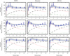 |
Fig. 5. Observed rotation curve (blue dots with ±1σ error bars) fit with the NFW (left), Einasto (middle), and DC14 (right) halo models. The model rotation curve (blue solid line with ±1σ error band) is decomposed into the contributions of stars (bulge plus disk; red dotted line), gas (atomic plus molecular; green dash-dotted line), and DM halo (black dashed line). |
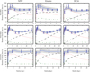 |
Fig. 6. Same as Fig. 5, but without cosmological priors imposed on the DM halo parameters in the fitting procedure. |
Maximum-probability values with ΛCDM constraints for the fit parameters.
When the ΛCDM priors are imposed, different halo profiles give nearly indistinguishable results for all galaxies. When we adopt uniform priors on the halo parameters, however, we find significant differences for NGC 3626. For this object, the rotation curve displays a strong decline at intermediate radii driven by the stars, followed by a nearly solid-body rise driven by the halo. The latter cannot be reproduced by a cuspy DM halo, like the NFW or the Einasto and DC14 with ΛCDM constraints, but it is well described by a cored DM halo, like Einasto with low α values and DC14 with intermediate X values. Thus, the rotation curve of NGC 3626 suggests that DM cores are not only a prerogative of low-mass galaxies, but they may exist in high-mass galaxies too, providing a challenge for current stellar-feedback models (Di Cintio et al. 2014) and possibly pointing to black-hole feedback shaping the inner DM halo (Macciò et al. 2020).
Figure 7 (top panels) illustrates that the maximum-probability halo parameters adhere well to the SHM relation (Moster et al. 2013) once it is imposed as a lognormal prior. For the DC14 profile, however, NGC 3626 is slightly offset to the right of the SHM relation because its rotation curve is pushing the fit toward low M⋆/M200 values in order to have a less cuspy DM profile. Figure 7 (bottom panels) shows that the halo parameters are also consistent with the imposed mass-concentration relation (Dutton & Macciò 2014) within the large uncertainties.
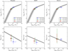 |
Fig. 7. Stellar-to-halo-mass relation (top) and halo mass-concentration relation (bottom). The black solid line and the gray shaded areas show the relations expected in ΛCDM together with their intrinsic scatter (Moster et al. 2013; Dutton & Macciò 2014). The solid points with ±1 sigma errorbars show the maximum-probability values from rotation-curve fits with ΛCDM priors. |
6. Discussion
6.1. Radial acceleration relation
Late type galaxies follow a tight radial acceleration relation (RAR; McGaugh 2016; Lelli et al. 2017): the observed centripetal acceleration at each radius correlates with that predicted by the baryonic components. This implies that, to a first approximation, the rotation-curve shape can be predicted by the baryon distribution, and vice versa. The scatter around the RAR is remarkably small for astronomical standards and is largely dominated by observational scatter, leaving little space for intrinsic scatter in the relation (Li et al. 2018, but see also Stone & Courteau 2019). In addition to the LTGs from the SPARC sample, Lelli et al. (2017) also considered 25 ETGs and 62 dwarf spheroidals, finding that they follow the same relation as LTGs (with the possible exception of ultra-faint dwarfs for which the observational situation is more uncertain). The RAR might represent a universal law of nature with severe implications on cosmological models (see Lelli et al. 2017 for a discussion).
Early type galaxies are the least represented galaxy type in the RAR. The sample of Lelli et al. (2017) included nine so-called slow rotators and 16 fast rotators (Cappellari et al. 2011b). The slow rotators are generally giant boxy ellipticals, in which the observed centripetal acceleration can be measured using X-ray halos in hydrostatic equilibrium (Buote & Humphrey 2012). The fast rotators comprise both disky ellipticals and lenticular galaxies: their inner circular velocities were estimated fitting Jeans axisymmetric models to the stellar kinematics (Cappellari et al. 2011b), while the outer circular velocities were measured using HI observations (den Heijer et al. 2015). Therefore, the mass models of these fast rotators were limited to two measured points only. Having derived full, extended rotation curves for rotating ETGs, we can more rigorously investigate their location on the RAR.
Following Lelli et al. (2017), we calculate the observed centripetal acceleration as  and the one predicted from the baryon distribution as
  with Υd = 0.5 and Υb = 0.7. Figure 8 shows that our ETGs lie on top of the RAR derived for LTGs within 1σ. Although our sample is too small to make statistically robust conclusions, this result suggests that galaxies follow the same RAR independently of their morphology and evolutionary stage. Thus, the rotation curves of ETGs can be predicted from the baryonic mass distribution using the same relation as for LTGs. This points to the possible universality of the RAR, in line with the predictions of Milgromian dynamics (MOND, Milgrom 1983). A bigger ETG sample with both CO and HI data is needed to reinforce this result.
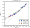 |
Fig. 8. RAR for our ETGs using Υd = 0.5 and Υb = 0.7 as in Lelli et al. (2017). Black and dashed lines correspond, respectively, to the mean and standard deviation of the RAR for LTGs in the SPARC database. The dotted line shows the 1:1 relation. |
6.2. Evolution of early-type galaxies
The dichotomy of early-type galaxies, dividing them into slow and fast rotators (e.g., Emsellem et al. 2007), is well established but the formation and evolution of the two galaxy types is subject of debate. The galaxies studied in this paper are rotating lenticulars, so we focus on their formation and evolution.
Several authors (e.g., Kormendy & Bender 2012; Laurikainen et al. 2010) proposed that lenticulars evolve from spirals through secular quenching of star formation, possibly driven by gas stripping and/or starvation (i.e., lack of gas accretion). These conclusions are motivated by the fact that the stellar disks and bulges of S0s follow the same photometric scaling relations as those of spirals. The fading scenario is backed from comparative population studies, showing that the fraction of LTGs decreases as a function of environmental density with nearly the same slope as the fraction of rotating ETGs increases (Cappellari et al. 2011b). Numerical simulations, however, show that lenticulars formed via major mergers may have coupled bulge-disk components that follow the same scaling relations as spirals (Querejeta et al. 2015), thus photometric data alone may not be sufficient to distinguish between secular fading and major mergers. In this evolutionary context, kinematical and dynamical studies acquire primary importance.
Rizzo et al. (2018) performed kinematic bulge-disk decompositions of unbarred S0s, separating the light contributions from bulge and disk at each spatial position of the optical spectrum. They found that the stellar disks of S0s have the same specific angular momentum as those of spirals, concluding that major mergers are not the dominant formation mechanisms for S0s in the group and field environments. Diametrically different conclusions are drawn by Falcón-Barroso et al. (2019), which, however, did not perform a kinematic bulge-disk decomposition of optical spectra but included bulges in their estimate of the specific stellar angular momentum. The results of our work, based on gas kinematics that is exempt from highly nontrivial spectral decompositions, give further support to the scenario in which S0s are forming from aging spiral galaxies in a fluent transition.
Figure 9 compares the rotation curves of ETGs with those of LTGs from SPARC (Lelli et al. 2016). The rotation-curve shapes of S0s are similar to spirals of comparable effective surface brightness and flat rotation velocity, hence they are of comparable baryonic mass (stars plus gas) since HI-rich ETGs follow the same baryonic Tully-Fisher relation as LTGs (den Heijer et al. 2015). This implies that the shape of the total gravitational potential is similar in spirals and lenticulars. Moreover, the amount of specific angular momentum in the gas disk of S0s is clearly similar to that of spirals, in analogy to the specific angular momentum in the stellar disk (Rizzo et al. 2018). Finally, our values for the mass-to-light ratios (0.5−0.7 M⊙/L⊙ at 3.6 μm) are lower than expected for old and passive ETGs with exponentially declining star-formation histories (0.8−1.0 M⊙/L⊙, see Fig. 11 in Schombert & McGaugh 2014), but are in the typical range of star-forming LTGs (Schombert et al. 2019). This suggests that the star-formation activity in our three ETGs must have dropped (if not stopped) only recently, which allows us to classify them as faded spirals.
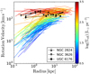 |
Fig. 9. Rotation curves of LTGs from the SPARC sample (Lelli et al. 2016) overlaid with the rotation curves of our ETGs. The LTG rotation curves are color-coded by their effective surface brightness at 3.6 μm. The location of the ETGs is consistent with their high effective surface brightnesses of ∼103 L⊙ pc−2. |
Our findings are consistent with those of Yıldız et al. (2017), who used a sample of HI-rich and HI-poor ETGs from the ATLAS3D survey to study their star-formation properties. They compared the UV colors of the two samples and found that HI-rich ETGs are bluer than HI-poor ETGs. The most gas-rich ETGs are as blue as the outer parts of typical LTGs. Yıldız et al. (2017) concluded that gas-rich ETGs host young stellar populations in their outskirts. They also found evidence of low star formation efficiency in these regions. Although our galaxies are not part of Yildiz’s sample, their HI mass places them among the gas-rich ETGs (NGC 2824 was not considered by Yıldız et al. (2017) due to the weak HI detection in the Atlas3D data, while NGC 3626 and UGC 6176 had no available UV observations). NGC 3626 likely has some ongoing star formation, possibly triggered by a recent interaction with its companion galaxy, as suggested by the stellar and gas rings visible in its outer disk.
Further support for a faded-spiral scenario comes from comparing our derived DM halo parameters to the ones for the LTGs in the SPARC sample (Li et al. 2019). This is shown in Fig. 10, where the halo scale length and characteristic densities are plotted versus the galaxy luminosity at 3.6 μm. The DM halos of our lenticular galaxies follow the same relations of SPARC galaxies within the errors. Thus, these ETGs live in similar DM halos as LTGs, indicating that they may be fading spirals. This also suggests that the evolution from spirals to lenticulars do not necessarily involve major structural changes in the DM halo, as one may expect after a major merger. Indeed, we can exclude major mergers in the recent past of our galaxies (1 − 2 Gyr). The orbital times in their outermost regions range from 0.3 to 0.8 Gyr: since the velocity fields are reasonably symmetric, the gas disk must have remained relatively unperturbed for several orbital times.
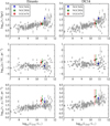 |
Fig. 10. DM halo parameters versus [3.6] luminosity for our three ETGs and the LTGs in the SPARC sample (gray dots from Li et al. 2019): halo scale radius (top panels), characteristic volume density (middle panels), and their product (bottom panels). |
7. Conclusion
We analyzed the dynamics of three S0s that have inner CO emission and outer, extended HI disks. This special feature allowed us to trace the rotation curve from the innermost parts of the galaxies out to 10−20 effective radii. We derived mass models using Spitzer photometry at 3.6 μm and performed DM halo fits. Then, we compared the properties of our ETGs with those of LTGs from the SPARC sample to constrain the evolutionary history of lenticular galaxies. We found the following results:
-
The rotation-curve shapes of our ETGs are similar to those of LTGs of similar mass and surface brightness. This is consistent with a smooth transition from spirals to lenticulars.
-
The dynamically inferred values of the stellar mass-to-light ratio are relatively small for passive ETGs. The retrieved values are similar to those of LTGs (0.5−0.7 M⊙/L⊙). This suggests recent star formation events in these galaxies, consistent with the picture of spirals slowly fading into lenticulars.
-
The DM halo parameters follow the same scaling relations with galaxy luminosity as those of LTGs. This suggests that the transition from LTGs to ETGs happened without altering the halo structure of the galaxies, for example, via a violent event like a major merger.
-
The rotation curve of NGC 3626 has a significant inner decline driven by the stars and a subsequent rise driven by the halo, which is poorly fit by cuspy DM profiles. This suggests that DM cores may exist in high-mass galaxies.
-
We confirm that ETGs follow the same radial acceleration relation as LTGs, pointing to the universality of this relation for galaxies of different morphologies and evolutionary stages.
Our results paint a consistent picture of the evolution of lenticular galaxies, which is in agreement with previous works. A bigger sample of gas-bearing ETGs is needed to make more general statements. Such a sample might be accessible in the near future thanks to new CO surveys with ALMA and NOEMA, as well as HI surveys with the SKA and its pathfinders.
There is a typo in Eq. (3) of Katz et al. (2017) since the factor 10−5 appears inside the exponential. The equation written here is the correct one, which was used in the analysis of Katz et al. (2017).
Acknowledgments
We thank the anonymous referee for a constructive report that improved the clarity of this paper. A.S. is grateful for the hospitality and financial support of Harvard University and the European Southern Observatory (Germany Headquarters), where most of this work was carried out. We are in debt to Paolo Serra for providing us with a deep HI cube of NGC 2824, Pengfei Li for sharing his rotation-curve fitting codes, and Enrico di Teodoro for crucial help with 3DBarolo. We also thank Ralph Bender, Michele Cappellari, Timothy Davis, Stacy McGaugh, and James Schombert for useful discussions. We acknowledge the Atlas3D survey team for making their datacubes publicly available. This research has made use of the NASA/IPAC Extragalactic Database (NED) which is operated by the Jet Propulsion Laboratory, California Institute of Technology, under contract with the National Aeronautics and Space Administration.
References
- Alatalo, K., Davis, T. A., Bureau, M., et al. 2013, MNRAS, 432, 1796 [NASA ADS] [CrossRef] [Google Scholar]
- Begeman, K. G. 1987, PhD Thesis, Kapteyn Institute [Google Scholar]
- Bershady, M. A., Verheijen, M. A. W., Westfall, K. B., et al. 2010, ApJ, 716, 234 [NASA ADS] [CrossRef] [Google Scholar]
- Bolatto, A. D., Wolfire, M., & Leroy, A. K. 2013, ARA&A, 51, 207 [Google Scholar]
- Buote, D. A., & Humphrey, P. J. 2012, in Dark Matter in Elliptical Galaxies, eds. D. W. Kim, & S. Pellegrini, Astrophys. Space Sci. Lib., 378, 235 [CrossRef] [Google Scholar]
- Buta, R. J., Sheth, K., Athanassoula, E., et al. 2015, VizieR Online Data Catalog: J/ApJS/217/32 [Google Scholar]
- Cappellari, M. 2016, ARA&A, 54, 597 [NASA ADS] [CrossRef] [Google Scholar]
- Cappellari, M., Emsellem, E., Krajnović, D., et al. 2011a, MNRAS, 413, 813 [NASA ADS] [CrossRef] [Google Scholar]
- Cappellari, M., Emsellem, E., Krajnović, D., et al. 2011b, MNRAS, 416, 1680 [NASA ADS] [CrossRef] [Google Scholar]
- Casertano, S., & van Gorkom, J. H. 1991, AJ, 101, 1231 [NASA ADS] [CrossRef] [Google Scholar]
- Ciri, R., Bettoni, D., & Galletta, G. 1995, Nature, 375, 661 [NASA ADS] [CrossRef] [Google Scholar]
- Davis, T. A., Alatalo, K., Bureau, M., et al. 2013, MNRAS, 429, 534 [NASA ADS] [CrossRef] [Google Scholar]
- de Grijs, R. 1998, MNRAS, 299, 595 [NASA ADS] [CrossRef] [Google Scholar]
- de Vaucouleurs, G., de Vaucouleurs, A., Corwin, H. G., Jr., et al. 1991, Third Reference Catalogue of Bright Galaxies (New York: Springer) [Google Scholar]
- den Heijer, M., Oosterloo, T. A., Serra, P., et al. 2015, A&A, 581, A98 [NASA ADS] [CrossRef] [EDP Sciences] [Google Scholar]
- Di Cintio, A., Brook, C. B., Dutton, A. A., et al. 2014, MNRAS, 441, 2986 [Google Scholar]
- Di Teodoro, E. M., & Fraternali, F. 2015, MNRAS, 451, 3021 [Google Scholar]
- Dutton, A. A., & Macciò, A. V. 2014, MNRAS, 441, 3359 [Google Scholar]
- Einasto, J. 1965, Trudy Astrofizicheskogo Instituta Alma-Ata, 5, 87 [NASA ADS] [Google Scholar]
- Emsellem, E., Cappellari, M., Krajnović, D., et al. 2007, MNRAS, 379, 401 [Google Scholar]
- Falcón-Barroso, J., van de Ven, G., Lyubenova, M., et al. 2019, A&A, 632, A59 [CrossRef] [EDP Sciences] [Google Scholar]
- Forbes, D. A., Alabi, A., Romanowsky, A. J., et al. 2016, MNRAS, 458, L44 [Google Scholar]
- Foreman-Mackey, D., Conley, A., Meierjurgen Farr, W., et al. 2013, Astrophysics Source Code Library [record ascl:1303.002] [Google Scholar]
- Gerhard, O. 2013, in The Intriguing Life of Massive Galaxies, eds. D. Thomas, A. Pasquali, & I. Ferreras, IAU Symp., 295, 211 [Google Scholar]
- Haynes, M. P., Jore, K. P., Barrett, E. A., Broeils, A. H., & Murray, B. M. 2000, AJ, 120, 703 [Google Scholar]
- Janz, J., Laurikainen, E., Laine, J., Salo, H., & Lisker, T. 2016, MNRAS, 461, L82 [Google Scholar]
- Jore, K. P., Haynes, M. P., & Broeils, A. H. 1996, Am. Astron. Soc. Meet. Abstr., 189, 68.04 [Google Scholar]
- Katz, H., Lelli, F., McGaugh, S. S., et al. 2017, MNRAS, 466, 1648 [Google Scholar]
- Kormendy, J., & Bender, R. 2012, ApJS, 198, 2 [Google Scholar]
- Kormendy, J., & Freeman, K. C. 2004, in Dark Matter in Galaxies, eds. S. Ryder, D. Pisano, M. Walker, & K. Freeman, IAU Symp., 220, 377 [Google Scholar]
- Laurikainen, E., Salo, H., Buta, R., Knapen, J. H., & Comerón, S. 2010, MNRAS, 405, 1089 [NASA ADS] [Google Scholar]
- Lelli, F., Verheijen, M., Fraternali, F., & Sancisi, R. 2012a, A&A, 537, A72 [NASA ADS] [CrossRef] [EDP Sciences] [Google Scholar]
- Lelli, F., Verheijen, M., Fraternali, F., & Sancisi, R. 2012b, A&A, 544, A145 [NASA ADS] [CrossRef] [EDP Sciences] [Google Scholar]
- Lelli, F., Verheijen, M., & Fraternali, F. 2014, MNRAS, 445, 1694 [Google Scholar]
- Lelli, F., McGaugh, S. S., & Schombert, J. M. 2016, AJ, 152, 157 [Google Scholar]
- Lelli, F., McGaugh, S. S., Schombert, J. M., & Pawlowski, M. S. 2017, ApJ, 836, 152 [Google Scholar]
- Li, P., Lelli, F., McGaugh, S., & Schombert, J. 2018, A&A, 615, A3 [NASA ADS] [CrossRef] [EDP Sciences] [Google Scholar]
- Li, P., Lelli, F., McGaugh, S. S., Starkman, N., & Schombert, J. M. 2019, MNRAS, 482, 5106 [Google Scholar]
- Li, P., Lelli, F., McGaugh, S., & Schombert, J. 2020, ApJS, 247, 31 [Google Scholar]
- Macciò, A. V., Crespi, S., Blank, M., & Kang, X. 2020, MNRAS, 495, L46 [Google Scholar]
- Mazzei, P., Marino, A., Rampazzo, R., Galletta, G., & Bettoni, D. 2014, Adv. Space Res., 53, 950 [Google Scholar]
- McGaugh, S. S. 2012, AJ, 143, 40 [Google Scholar]
- McGaugh, S. S. 2016, ApJ, 816, 42 [Google Scholar]
- McGaugh, S. S., Lelli, F., & Schombert, J. M. 2020, Res. Notes Am. Astron. Soc., 4, 45 [Google Scholar]
- Milgrom, M. 1983, ApJ, 270, 365 [NASA ADS] [CrossRef] [Google Scholar]
- Moster, B. P., Naab, T., & White, S. D. M. 2013, MNRAS, 428, 3121 [Google Scholar]
- Navarro, J. F., Frenk, C. S., & White, S. D. M. 1996, ApJ, 462, 563 [NASA ADS] [CrossRef] [Google Scholar]
- Noordermeer, E. 2008, MNRAS, 385, 1359 [Google Scholar]
- Noordermeer, E., van der Hulst, J. M., Sancisi, R., Swaters, R. S., & van Albada, T. S. 2007, MNRAS, 376, 1513 [NASA ADS] [CrossRef] [Google Scholar]
- Querejeta, M., Eliche-Moral, M. C., Tapia, T., et al. 2015, A&A, 579, L2 [NASA ADS] [CrossRef] [EDP Sciences] [Google Scholar]
- Rizzo, F., Fraternali, F., & Iorio, G. 2018, MNRAS, 476, 2137 [NASA ADS] [CrossRef] [Google Scholar]
- Schombert, J., & McGaugh, S. 2014, PASA, 31, e036 [Google Scholar]
- Schombert, J., McGaugh, S., & Lelli, F. 2019, MNRAS, 483, 1496 [NASA ADS] [Google Scholar]
- Serra, P., Oosterloo, T., Morganti, R., et al. 2012, MNRAS, 422, 1835 [Google Scholar]
- Sil’chenko, O. K., Moiseev, A. V., & Shulga, A. P. 2010, AJ, 140, 1462 [Google Scholar]
- Starkman, N., Lelli, F., McGaugh, S., & Schombert, J. 2018, MNRAS, 480, 2292 [Google Scholar]
- Stone, C., & Courteau, S. 2019, ApJ, 882, 6 [Google Scholar]
- Struve, C., Oosterloo, T., Sancisi, R., Morganti, R., & Emonts, B. H. C. 2010, A&A, 523, A75 [NASA ADS] [CrossRef] [EDP Sciences] [Google Scholar]
- van Albada, T. S., & Sancisi, R. 1986, Philos. Trans. R. Soc. London Ser. A, 320, 447 [Google Scholar]
- van Albada, T. S., Bahcall, J. N., Begeman, K., & Sancisi, R. 1985, ApJ, 295, 305 [Google Scholar]
- van der Hulst, J. M., Terlouw, J. P., Begeman, K. G., Zwitser, W., & Roelfsema, P. R. 1992, in The Groningen Image Processing SYstem, GIPSY, eds. D. M. Worrall, C. Biemesderfer, & J. Barnes, ASP Conf. Ser., 25, 131 [Google Scholar]
- Verheijen, M. A. W., & Sancisi, R. 2001, A&A, 370, 765 [NASA ADS] [CrossRef] [EDP Sciences] [Google Scholar]
- Weijmans, A.-M., Krajnović, D., van de Ven, G., et al. 2008, MNRAS, 383, 1343 [Google Scholar]
- Yıldız, M. K., Serra, P., Peletier, R. F., Oosterloo, T. A., & Duc, P.-A. 2017, MNRAS, 464, 329 [Google Scholar]
Appendix A: Notes on individual galaxies
In this appendix, we present in detail the results of our 3D kinematic modeling with GALMOD and 3DBAROLO (see Sect. 3). For each galaxy, we describe intensity maps, position-velocity (PV) diagrams, and channel maps for both HI and CO emissions. The figures are structured in a uniform way.
A.1. NGC 2824
The observed HI intensity map is well reproduced by our model (Fig. A.1, top panels) apart from an over-denstiy in the northern half of the disk, visible in the residual map, that cannot be reproduced by an axisymmetric disk. The observed PV diagrams display negative signal toward the galaxy center, associated to HI absorption, that our model cannot reproduce (Fig. A.1, bottom panels). Apart from these shortcomings, the HI kinematics are well reproduced. This is confirmed by Fig. A.2 comparing HI channel maps from the observed and model cubes.
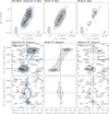 |
Fig. A.1. Top panels: HI intensity maps from the observed cube (left), model cube (middle) and residual cube (right) of NGC 2824. The cross and the dashed line indicate the galaxy center and position angle, respectively. The beam is shown in the bottom left corner. The physical scale is illustrated in the bottom right corner. The contours correspond to 3σpseudo, 6σpseudo, and so on. The outermost contour of the model is plotted in blue over the observed intensity map for comparison. Bottom panels: position-velocity diagrams taken along the major and minor axes from the observed cube (left), model cube (middle) and residual cube (right). The white squares show our derived rotation curve. The outermost contour of the model is plotted in blue over the observed PV diagrams for comparison. The density contours in the PV diagrams correspond to −1.5σ, −3σ (dashed) and 1.5σ, 3σ, 6σ, and so on (solid), where σ is the measured noise in the cube (see Table 2). |
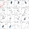 |
Fig. A.2. HI channel maps for NGC 2824 from the observed cube (gray scale) and the model cube (blue contours). The line-of-sight velocity is shown in the upper left corner. The cross indicates the galaxy center. The contours correspond to −3σ, −1.5σ (dashed) and 1.5σ, 3σ, 6σ, and so on (solid). In the first panel, the red contours correspond to arbitrary isophotes of the Spitzer image at 3.6 μm, the beam is shown in the bottom-left corner, and the physical scale is given in the bottom-right corner. |
The observed CO density maps indicates that the molecular disk is lopsided, extending farther toward the approaching part of the galaxy. This feature cannot be fully reproduced by our axisymmetric model (Fig. A.3, top panels). This also causes asymmetries in the PV diagrams (Fig. A.3, bottom panels). In our modeling, we give more weight to the extended, approaching half of the CO disk. Figure A.4 shows that the observed CO channel maps are well reproduced by our model.
A.2. NGC 3626
NGC 3626 is connected to the companion galaxy UGC 6341 by a diffuse HI bridge (Fig. A.5, top panels). We model only the HI emission associated to the disk of NGC 3626. The residual map shows that our axisymmetric model reproduces the HI disk very well, except for a ring feature at R ≃ 3′. The major-axis PV diagram shows a prominent dip (Fig. A.5, bottom panels): since this feature is observed on both sides of the galaxy, we consider it an intrinsic feature of the rotation curve rather than an effect of noncircular motions. Overall, the HI kinematics is well reproduced, as shown by the channel maps in Fig. A.6.
The CO distribution is quite asymmetric (Fig. A.7, top panels), but this is likely due to the fact that the CO observations did not cover the full frequency range of galaxy emission, as can be appreciated by the sharp cutoff of the PV diagrams at low velocities (Fig. A.7, bottom panels). In our modeling, we manually adjust the rotation curve to reproduce the receding part of the galaxy. The resulting model also reproduces the approaching half, including the nonmeasured part of it. The channels maps in Fig. A.8 further demonstrate that the CO kinematics is well reproduced by our model.
The CO data confirms the strong decline in the inner parts of the rotation curve. Even in the extreme case of an edge-on CO disk (which is clearly not the case as seen in Fig. A.7), the CO rotation velocities at small radii are higher than the HI rotation velocities at large radii. Our rotation curve is about 50 km s−1 higher in the inner parts than the one presented in Mazzei et al. (2014). We stress the HI disk is warped and the variations of i and PA with radius are not well constrained by the data. At small radii, we adopt the values of i and PA suggested by the CO disk, then we assume a simple linear rise to the higher values of i and PA suggested by the HI disk at large radii. Clearly, a different modeling of the warp may slightly change the shape of the rotation curve and the resulting stellar mass-to-light ratios.
A.3. UGC 6176
The HI distribution and kinematics are regular and symmetric, so they are well described by our axisymmetric model (Figs. A.9 and A.10). We note, however, that the HI disk is poorly resolved and beam-smearing effects are severe, leading to a very broad PV diagram along the minor axis.
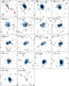 |
Fig. A.10. Same as Fig. A.2, but for the HI data of UGC 6176. |
The CO disk is even less resolved than the HI emission, so we have only one ring in our model (Fig. A.11). The beam is elongated along the east-west direction leading to nontrivial beam-smearing effects. We could not properly reproduce the axial ratio of the observed CO map for any value of the disk inclination. We suspect that the CO beam is not Gaussian, so our model cannot reproduce such extreme beam-smearing effects. In the end, we adopted a relatively high inclination of 85°, which gives the closest match to the observed CO map. At any rate, the observed PV diagrams are well described by our model. The CO channel maps are also reasonably reproduced (Fig. A.12).
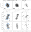 |
Fig. A.11. Same as Fig. A.1, but for the CO data of UGC 6176. |
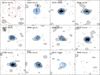 |
Fig. A.12. Same as Fig. A.2, but for the CO data of UGC 6176. |
Although the ATLAS3D collaboration denotes UGC 6176 as a warped galaxy, we find no strong evidence for it. The PA of the HI and the CO disks are consistent with each other and show no clear variation with radius, while the inclination of the CO disk cannot be properly assessed from the available data.
Appendix B: Posterior distributions of DM halo fits
In this appendix, we show the posterior distributions of the free parameters from DM halo fits with and without ΛCDM priors (see Sect. 5.1). When imposing ΛCDM priors (left panels), the posterior distributions are well-behaved and reasonably symmetric. Without imposing ΛCDM priors (right panels), the posterior distributions of the halo parameters become very complex, so their maximum-probability values are not fully trustworthy.
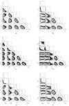 |
Fig. B.1. Posterior distributions for the DM halo fits of NGC 2824, with (left column) and without (right column) ΛCDM priors (see Sect. 5.1 for details). (a) NFW, (b) NFW (no priors), (c) Einasto, (d) Einasto (no priors), (e) DC14, and (f) DC14 (no priors). |
All Tables
All Figures
|
Fig. 1. Moment maps for NGC 2824 (left), NGC 3626 (middle), and UGC 6176 (right). The top section shows the HI data, while the bottom section shows the CO data. In each section, the top row shows the Spitzer image at 3.6 μm overlaid with the gas intensity maps, while the bottom row shows the velocity field. The box in the HI velocity field depicts the size of the CO frame. The cross corresponds to the galaxy center; the dashed line indicates the kinematic major axis; the physical scale is illustrated in the bottom-right corner; the beam shape is shown in the bottom-left corner. The HI and CO density contours are multiples of the pseudo-3σ value (0.5, 1, 2, 4, ...) where 3σmap is given in Table 2. |
| In the text | |
|
Fig. 2. Major-axis PV diagrams from the observed HI cube (top row) and the CO one (bottom row), overlaid with the projected rotation curve (white squares) and model PV diagrams (blue contour corresponding to 1.5σ from Table 2). |
| In the text | |
|
Fig. 3. Position angle (top), inclination (middle), and final rotation curves (bottom) from HI (green points) and CO (blue triangles) observations. Open circles show omitted points in the combined rotation curves due to the overlap of CO and HI data. |
| In the text | |
|
Fig. 4. Top panels: surface density profiles for the H2 disk (blue circles), HI disk (green upward triangles), stellar disk (yellow downward triangles), and stellar bulge (red diamonds) when necessary. Open circles indicate that the surface density is extrapolated from an exponential fit. Bottom panels: observed rotation curve (dots with ±1σ error bars) is fit with a maximum-disk mass models (black solid line with ±1σ error band). The baryonic rotation curve is decomposed into the contributions of molecular gas (blue dashed line), atomic gas (green dash-dotted line), stellar disk (yellow solid line), and stellar bulge (red dotted line) when necessary. The maximum mass-to-light ratios are given in the top right corner. |
| In the text | |
|
Fig. 5. Observed rotation curve (blue dots with ±1σ error bars) fit with the NFW (left), Einasto (middle), and DC14 (right) halo models. The model rotation curve (blue solid line with ±1σ error band) is decomposed into the contributions of stars (bulge plus disk; red dotted line), gas (atomic plus molecular; green dash-dotted line), and DM halo (black dashed line). |
| In the text | |
|
Fig. 6. Same as Fig. 5, but without cosmological priors imposed on the DM halo parameters in the fitting procedure. |
| In the text | |
|
Fig. 7. Stellar-to-halo-mass relation (top) and halo mass-concentration relation (bottom). The black solid line and the gray shaded areas show the relations expected in ΛCDM together with their intrinsic scatter (Moster et al. 2013; Dutton & Macciò 2014). The solid points with ±1 sigma errorbars show the maximum-probability values from rotation-curve fits with ΛCDM priors. |
| In the text | |
|
Fig. 8. RAR for our ETGs using Υd = 0.5 and Υb = 0.7 as in Lelli et al. (2017). Black and dashed lines correspond, respectively, to the mean and standard deviation of the RAR for LTGs in the SPARC database. The dotted line shows the 1:1 relation. |
| In the text | |
|
Fig. 9. Rotation curves of LTGs from the SPARC sample (Lelli et al. 2016) overlaid with the rotation curves of our ETGs. The LTG rotation curves are color-coded by their effective surface brightness at 3.6 μm. The location of the ETGs is consistent with their high effective surface brightnesses of ∼103 L⊙ pc−2. |
| In the text | |
|
Fig. 10. DM halo parameters versus [3.6] luminosity for our three ETGs and the LTGs in the SPARC sample (gray dots from Li et al. 2019): halo scale radius (top panels), characteristic volume density (middle panels), and their product (bottom panels). |
| In the text | |
|
Fig. A.1. Top panels: HI intensity maps from the observed cube (left), model cube (middle) and residual cube (right) of NGC 2824. The cross and the dashed line indicate the galaxy center and position angle, respectively. The beam is shown in the bottom left corner. The physical scale is illustrated in the bottom right corner. The contours correspond to 3σpseudo, 6σpseudo, and so on. The outermost contour of the model is plotted in blue over the observed intensity map for comparison. Bottom panels: position-velocity diagrams taken along the major and minor axes from the observed cube (left), model cube (middle) and residual cube (right). The white squares show our derived rotation curve. The outermost contour of the model is plotted in blue over the observed PV diagrams for comparison. The density contours in the PV diagrams correspond to −1.5σ, −3σ (dashed) and 1.5σ, 3σ, 6σ, and so on (solid), where σ is the measured noise in the cube (see Table 2). |
| In the text | |
|
Fig. A.2. HI channel maps for NGC 2824 from the observed cube (gray scale) and the model cube (blue contours). The line-of-sight velocity is shown in the upper left corner. The cross indicates the galaxy center. The contours correspond to −3σ, −1.5σ (dashed) and 1.5σ, 3σ, 6σ, and so on (solid). In the first panel, the red contours correspond to arbitrary isophotes of the Spitzer image at 3.6 μm, the beam is shown in the bottom-left corner, and the physical scale is given in the bottom-right corner. |
| In the text | |
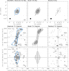 |
Fig. A.3. Same as Fig. A.1, but for the CO data of NGC 2824. |
| In the text | |
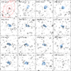 |
Fig. A.4. Same as Fig. A.2, but for the CO data of NGC 2824. |
| In the text | |
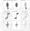 |
Fig. A.5. Same as Fig. A.1, but for the HI data of NGC 3626. |
| In the text | |
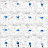 |
Fig. A.6. Same as Fig. A.2, but for the HI data of NGC 3626. |
| In the text | |
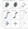 |
Fig. A.7. Same as Fig. A.1, but for the CO data of NGC 3626. |
| In the text | |
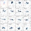 |
Fig. A.8. Same as Fig. A.2, but for the data CO of NGC 3626. |
| In the text | |
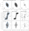 |
Fig. A.9. Same as Fig. A.1, but for the HI data of UGC 6176. |
| In the text | |
|
Fig. A.10. Same as Fig. A.2, but for the HI data of UGC 6176. |
| In the text | |
|
Fig. A.11. Same as Fig. A.1, but for the CO data of UGC 6176. |
| In the text | |
|
Fig. A.12. Same as Fig. A.2, but for the CO data of UGC 6176. |
| In the text | |
|
Fig. B.1. Posterior distributions for the DM halo fits of NGC 2824, with (left column) and without (right column) ΛCDM priors (see Sect. 5.1 for details). (a) NFW, (b) NFW (no priors), (c) Einasto, (d) Einasto (no priors), (e) DC14, and (f) DC14 (no priors). |
| In the text | |
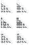 |
Fig. B.2. Same as Fig. B.1, but for NGC 3626. |
| In the text | |
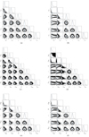 |
Fig. B.3. Same as Fig. B.1, but for UGC 6176. |
| In the text | |
Current usage metrics show cumulative count of Article Views (full-text article views including HTML views, PDF and ePub downloads, according to the available data) and Abstracts Views on Vision4Press platform.
Data correspond to usage on the plateform after 2015. The current usage metrics is available 48-96 hours after online publication and is updated daily on week days.
Initial download of the metrics may take a while.