Constraining the parameter space for the solar nebula

Christian T. Lenz; Hubert Klahr; Tilman Birnstiel; Katherine Kretke; Sebastian Stammler

doi:10.1051/0004-6361/202037878

Home

All issues

Volume 640 (August 2020)

A&A, 640 (2020) A61

Full HTML

Open Access

Issue		A&A Volume 640, August 2020


Article Number		A61
Number of page(s)		21
Section		Interstellar and circumstellar matter
DOI		https://doi.org/10.1051/0004-6361/202037878
Published online		12 August 2020

A&A 640, A61 (2020)

The effect of disk properties on planetesimal formation

Christian T. Lenz¹^,★, Hubert Klahr¹, Tilman Birnstiel², Katherine Kretke³ and Sebastian Stammler²

¹ Max Planck Institute for Astronomy, Königstuhl 17, 69117 Heidelberg, Germany
e-mail: lenz@mpia.de, klahr@mpia.de
² University Observatory, Faculty of Physics, Ludwig-Maximilians-Universität München, Scheinerstr. 1, 81679 Munich, Germany
³ Southwest Research Institute, 1050 Walnut Ave, Suite 300, Boulder, CO 80302, USA

Received: 4 March 2020
Accepted: 22 May 2020

Abstract

Context. When we wish to understand planetesimal formation, the only data set we have is our own Solar System. The Solar System is particularly interesting because so far, it is the only planetary system we know of that developed life. Understanding the conditions under which the solar nebula evolved is crucial in order to understand the different processes in the disk and the subsequent dynamical interaction between (proto-)planets after the gas disk has dissolved.

Aims. Protoplanetary disks provide a plethora of different parameters to explore. The question is whether this parameter space can be constrained, allowing simulations to reproduce the Solar System.

Methods. Models and observations of planet formation provide constraints on the initial planetesimal mass in certain regions of the solar nebula. By making use of pebble flux-regulated planetesimal formation, we performed a parameter study with nine different disk parameters such as the initial disk mass, the initial disk size, the initial dust-to-gas ratio, the turbulence level, and others.

Results. We find that the distribution of mass in planetesimals in the disk depends on the timescales of planetesimal formation and pebble drift. Multiple disk parameters can affect the pebble properties and thus planetesimal formation. However, it is still possible to draw some conclusions on potential parameter ranges.

Conclusions. Pebble flux-regulated planetesimal formation appears to be very robust, allowing simulations with a wide range of parameters to meet the initial planetesimal constraints for the solar nebula. This means that it does not require much fine-tuning.

Key words: accretion, accretion disks / protoplanetary disks / circumstellar matter / turbulence / methods: numerical / minor planets, asteroids: general

^★

Member of the International Max Planck Research School for Astronomy and Cosmic Physics at the Heidelberg University.

© C. T. Lenz et al. 2020

Open Access article, published by EDP Sciences, under the terms of the Creative Commons Attribution License (http://creativecommons.org/licenses/by/4.0), which permits unrestricted use, distribution, and reproduction in any medium, provided the original work is properly cited.

Open Access funding provided by Max Planck Society.

1 Introduction

In order to form planets, tiny micron-sized dust grains have to grow to hundreds or thousands of kilometers. First, grains grow by collisions with other grains. At some point, however, they cannot continue to grow because either (1) the relative velocities become so high that a collision leads to fragmentation (Blum & Münch 1993; Blum & Wurm 2008; Gundlach & Blum 2014), or (2) they start to drift faster toward the star than they could potentially grow (Klahr & Bodenheimer 2006; Birnstiel et al. 2012). There is also the bouncing barrier (Zsom et al. 2010), but charging effects might lead to a growth to sizes that are an order of magnitude above the limit of this barrier (Steinpilz et al. 2019). Laboratory experiments point in the direction of low fragmentation speeds for icy particles (Musiolik & Wurm 2019) of around 1 m s⁻¹. This might cause particles to hit the fragmentation barrier first, which is why we do not consider bouncing in this paper.

Planets are thought to be formed by so-called planetesimals, which have sizes of a few to hundreds of kilometers. These planetesimals are the building blocks of planets. After they have formed, accretion of pebbles (Ormel & Klahr 2010) may become important as well (for a review see, e.g., Ormel 2017). Because grains stop growing at some point, however, continuous growth leaves a missing link between diameters of roughly millimeter–decimeter to planetesimal size (~100 km) through continuous growth.

If there is a pressure bump in the disk, for instance, caused by a vortex or zonal flow, particles can become trapped around the center of the bump (Whipple 1972; Barge & Sommeria 1995). After the accumulation of enough pebbles, the streaming instability (Youdin & Goodman 2005) might be the dominant turbulent process that triggers fragmentation in the laminar case (α_t = 0). Alternatively, gravoturbulent planetesimal formation can occur in the turbulent case (α_t > 0) (Johansen et al. 2006, 2007).

To summarize, we follow the idea that pebbles form planetesimals in a gravoturbulent process leading to a Gaussian-like size distribution of planetesimals that peaks around 100 km in diameter (Klahr & Schreiber 2015; Schreiber 2018). These planetesimals can then build planetary embryos, which can grow by further accretion of both planetesimals and pebbles to form (proto-)planets.

The initial distribution of planetesimals is one of the greatest unknowns in planet formation models. The radial distribution in the disk is important for embryo formation and subsequent accretion of planetesimals onto embryos. While we can observe protoplanetary disks and debris disks around other stars, we cannot observe planetesimal populations. For only one system do we have relatively good knowledge of the present-day small body population: the Solar System. This system has also been modeled most frequently, therefore the strongest constraints we have on the initial planetesimal population comes from our Solar System, even though(as we discuss here) there are many uncertainties. The so-called minimum mass solar nebula (MMSN; Weidenschilling 1977a; Hayashi 1981) is the most commonly used assumption, but it is not based on a modern understanding of planet formation.

Lenz et al. (2019) presented a pebble flux-regulated model for the planetesimal formation rate. In this model, a spatial planetesimal distribution evolves with time and leads to a physically motivated planetesimal density disk profile. It may therefore be sensible to ask whether this model fits the constraints of our Solar System, and if so, how finely tuned it has to be.

This paper is structured as follows. In Sect. 2 we discuss possible constraints for initial planetesimals in different regions of the solar nebula. Section 3 describes the model we used. Section 4 presents the results, and we conclude in Sect. 5.

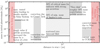Fig. 1

Graphical representation summarizing Sect. 2 on mass constraints of initial planetesimal masses in different regions of the solar nebula. Masses given by the values on the ordinate apply for the entire marked regions. Boxes that extend to the border of the plot indicate unknown upper limits. The dotted vertical line separates the two touching regions.

2 Mass constraints for the initial planetesimal population

In this section we review literature studies to infer constraints on the initial planetesimal mass in various regions of the solar nebula. A summary of this literature research is depicted in Fig. 1.

2.1 Mercury region: interior to 0.7 au

There is no observed stable population of asteroids within the orbit of Mercury (Steffl et al. 2013), even though Campins et al. (1996) for example found a dynamically stable region in the inner region of the Solar System. Moreover, no models for terrestrial planet formation require any planetesimals inside of the Mercury orbit (~ 0.4 au). Additionally, terrestrial planet models fit observations better when the planetesimal disk is truncated around 0.7 AU (Hansen 2009; Walsh et al. 2011; Levison et al. 2015; Morbidelli et al. 2016). Even though some models have suggested a mechanism that might clear out this region (e.g., Ida & Lin 2008; Batygin & Laughlin 2015; Volk & Gladman 2015), none of these are demonstrated in a comprehensive way. However, this implies that we cannot define an upper limit on the mass of initial planetesimals in this region. Low-mass short-period planets around other stars may indicate that other planetary systems contained planetesimals on short-period orbits that formed planets by in situ planetesimal accretion (e.g., Chiang & Laughlin 2013; Hansen & Murray 2012) or pebble accretion (e.g., Chatterjee & Tan 2013), but migration implies that there is no evidence that a population of initial planetesimals was present within the Mercury orbit in our own Solar System. In conclusion, in this region the mass limits span from zero to an unknown upper limit. This implies that there is no necessity to form planetesimals initially in this region.

2.2 Earth-to-Venus region 0.7–1 au

As was shown by Hansen (2009), placing ~2 M_⊕ of oligarchs within 0.7−1 au can lead to good matches to the sizes and spacing of the terrestrial planets of the Solar System. The results from the parameter study of Kokubo et al. (2006) in terms of the number of Earth-like planets within 0.5 to 1.5 au appear to be very robust with respect to the mass and radial profile of oligarchs. The authors showed that reasonable results can still be obtained with a total initial mass of 2.77 M_⊕ in this region. For ~23 M_⊕, super-Earths form.

Pebble flux can allow a significant amount of mass to be transported into this region. When there are enough pebbles and an appropriate disk structure, it is possible to produce reasonable Solar System analogs beginning with < 10⁻² M_⊕ planetesimal masses (Levison et al. 2015). For Jupiter to leave about the mass required in the current asteroid belt, Jupiter would have had to migrate inward and then out of the asteroid belt (known as the grand tack; Walsh et al. 2011) and would have implanted ~ 1 M_⊕ of material into the Earth-Venus-forming region. This suggests that either primordially or after early pebble accretion, there was initially 1 M_⊕ of planetesimals or embryos in this region (Walsh et al. 2011). Because the grand tack removes most objects in the asteroid belt in simulations, the initial planetesimal population needs to be massive enough early on. This probably implies that pebble accretion only grew the mass of the asteroid belt by a factor of a few at most, and thus the terrestrial planet region probably only grew by a factor of a few as well. As a rough estimate, we can assume that the inital planetesimal mass is about 0.1 M_⊕. In conclusion, in this region the mass limits are between 0.1 (if there are enough pebbles that can be accreted) and 2.77 M_⊕ (if there are not).

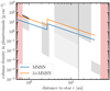Fig. 2

As Fig. 1, but converted into column densities, assuming a power-law shape ∝ r^−2.25 (see Eq. (37) of Lenz et al. 2019 for a motivation). The blue (orange) line shows (three times) the minimum mass solar nebula profile for solids (Weidenschilling 1977a; Hayashi 1981).

2.3 Asteroid belt: 2–3 au

The asteroid belt currently has a mass of about 5 × 10⁻⁴ M_⊕ (e.g., Kresak 1977), where roughly 50% of the mass resides in the four largest objects, with 1/3 in Ceres. Over the history of the Solar System, it has potentially been depleted by the following effects: (1) over the past 4 Gyr, dynamical chaos in the current structure of the Solar System has removed about 50% of the mass of the asteroid belt (Minton & Malhotra 2010). The Vesta crust indicates that the asteroid belt population was only modestly larger at the time when the mean collision velocities were pumped up to 5 km s⁻¹ (i.e., the current mean impact velocity in the main belt region; Bottke et al. 1994) than it is today. If the asteroid belt contained substantially more planetesimals with sizes of 30 km over the last 4 Gyr than it has today, Vesta would be expected to have more than one large basin (Bottke et al. 2005a,b; O’Brien & Greenberg 2005). If planetesimals were “born big” (Morbidelli et al. 2009), that is, ≳ 80 km, this suggests that collisional evolution should not be particularly important in removing material; at least not more than a factor of a few. The late Jupiter-Saturn interaction in terms of a reshuffling of the giant planets likely depleted the asteroid belt by a factor of ~ 2 to ~ 10 (Minton & Malhotra 2010). If the grand tack occurred (Walsh et al. 2011), then only a few times 10⁻³ to a few times 10⁻⁴ of the population would have survived (ignoring newly implanted planetesimals from other regions; see, e.g., Fig. 7 in Morbidelli et al. 2015). Moreover, in the model used by Morbidelli et al. (2015) the C-complex asteroids, which comprise about 75% of the asteroids (Gradie et al. 1989) and include Ceres, are implanted from the outer Solar System. These modifications are swamped by the uncertainty in the clearing rate on the migration efficiency, however. If pebble accretion plays a crucial role for the growth of large asteroids (>200 km in diameter), then this also would reduce the “initial mass” of planetesimals that is needed. This effect probably would be a factor of ~ 2 (Johansen et al. 2015). In conclusion, in this region the limits for the initial planetesimal mass lie between ~ 2 ×10⁻³ M_⊕ (four times the current mass) and ~5 M_⊕.

2.4 Giant-planet-forming region (possibly) 4–15 au

The region in which giant planets form could also have an inner (outer) edge that is farther in (out). This would not change the constraints by much, however.

The lower mass limit of the Saturn core is about 8−9 M_⊕ (Saumon & Guillot 2004; Helled & Schubert 2008), and the Jupiter core has at least 7 M_⊕ (Wahl et al. 2017). So far, we do not know how much of this mass was originally contained in planetesimals from the appropriate region. For the lower limit, we therefore ignore Saturn and take 50% (assuming that the other half stems from pebbles, Bordukat 2019) of the lower mass estimate from Wahl et al. (2017), which gives 3.5 M_⊕.

In order to reach critical masses for strong gas accretion, about five times the mass of the MMSN seems to be needed (Thommes & Duncan 2006, these simulations used planetesimals of 20 km in diameter). This leads to 132 M_⊕ within 4 to 15 au. Assuming that 50% of the mass was contributed by pebbles (Bordukat 2019), the lower limit would be about 66 M_⊕. This lower limit is still high, but desublimation effects just outside the ice line can lead to a pileup in planetesimals by a factor of ~ 5 (Drążkowska & Alibert 2017; Schoonenberg et al. 2018). This effect is not included in this work.

Raymond & Izidoro (2017) found that ~10% of the asteroids around the giant planets were scattered into the asteroid belt. In order to explain the mass of C-type asteroids in the asteroid belt, therefore probably about a few times 10⁻² M_⊕ of asteroids had to have been in the giant-planet-forming region. This value would be the absolute minimum for this region. We conclude that the possible initial planetesimal mass was at least ~ 66 M_⊕ with an unknownhigh mass as upper limit.

2.5 Nice disk ~15–30 au

In order to match the observed structure of the Kuiper belt, where many objects are in resonance with Neptune, outward migration of the giant planets is the preferred explanation. For this type of outward migration, planetesimal-driven migration isthe leading explanation (Fernandez & Ip 1984; Malhotra 1995; Thommes et al. 1999). The Nice model (Tsiganis et al. 2005; Morbidelli et al. 2005; Gomes et al. 2005) is a comprehensive model that explains how this outward planetesimal-driven migration could have occurred. In this model the giant planets initially formed closer to the Sun than their current locations, and migrated outward as a result of interactions with a planetesimal disk known as the Nice disk. Even though the details of the model have been changed (e.g., Morbidelli et al. 2007; Levison et al. 2011), a number of features in the small-body reservoirs of our Solar System can be explained if this population did initially exist and the planets migrated through it. We give a few examples:

Jupiter Trojans: calculations showed that a mass of around ~35 M_⊕ can agree with the current population of the Jupiter Trojans (Morbidelli et al. 2005). With a newer variation, known as the jumping Jupiter model, good matches are found with planetesimal disk masses ~ 14−28 M_⊕ (Nesvornỳ et al. 2013).
Kuiper belt: models with grainy migration of Neptune with a disk mass of ~20 M_⊕ (1000 Pluto-sized objects) match the detailed characteristics of the objects in the 3:2 resonance (Nesvornỳ & Vokrouhlickỳ 2016).
Comets:gas drag prevents kilometer-sized planetesimals from being scattered into the Oort Cloud while the gas disk stillexists (Brasser et al. 2007). This suggests that the long-period comets were scattered into the Oort cloud after the gas disk vanished, a natural outcome of a model like the Nice model. An initial population of about 30 M_⊕ is needed to populate the Oort Cloud (Dones et al. 2004), but the existence of more massive planets in the inner Oort Cloud (e.g., a planet 9, Batygin & Brown 2016) could decrease the required reservoir size. However, because comets might have been shared between stars in the birth cluster under favorable conditions, it is possible that comets are not a reliable constraint (Levison et al. 2010).
Ice giant ejection: in the models in which an ice giant is ejected from the Solar System, the best overall structure of the Solar System, for example, surviving terrestrial planets, needs ~20 M_⊕ in planetesimals (Nesvornỳ & Morbidelli 2012).

Additionally, it has been found that the column density profile of planetesimals has a very weak effect on the outcomes for a relatively broad range of power laws. This was tested by Batygin & Brown (2010) for Σ_p ∝ r^−k, where k = 1…2, with inner edge r_in ~ 12 au and outer radius r_out = 30 au. The Nice scattering occurred after the disk has dissolved so that pebble accretion could have increased the total mass of the Nice disk. However, because the disk was very likely flaring in the outer regions, it is unlikely that pebble accretion was efficient and increased the total mass in these regions by more than a factor of ~ 2 (Lambrechts & Johansen 2012). To summarize, ~10 M_⊕ seems to be needed in this region.

2.6 Cold classical Kuiper belt ~30–50 au

There is a population of objects in the Kuiper belt with low eccentricities and inclinations that appear as though they are not transplanted, but are likely primordial. Observations indicate that the mass of the current classical population is 8 × 10⁻³ M_⊕ (Fuentes & Holman 2008).

If the larger KBOs were formed by coagulation from small planetesimals, there must have been significantly more mass in this region in the early stages. For instance, Pan & Sari (2005) suggested that the high-end size distribution could be matched by collisional evolution. However, when more modern description laws are combined with the requirment of preserving wide binaries, the observed population in this type of collisional environment cannot be match. This therefore suggests that planetesimals formed as large bodies and that the total mass of the cold classcial Kuiper belt objects (CKBOs), dominated by bodies larger than diameters of ~ 100 km, has not evolved significantly (Nesvornỳ et al. 2011).

The Nice migration may have dynamically depleted the Kuiper belt by up to an order of magnitude (Morbidelli et al. 2008). Singer et al. (2019) found a lack of small craters on Pluto and Charon, indicating that planetesimals in the Kuiper belt are not a collisionally evolved population, or that collisions destroyed small planetesimals. We conclude that the initial mass in planetesimals was between approximately 0.008 and ~ 0.1 M_⊕.

2.7 Beyond 50 au

A radial distance of approximately 50 au appears to be a real edge to the cold classical Kuiper belt (Jewitt et al. 1998; Trujillo & Brown 2001; Fuentes & Holman 2008). If there is a population with similar size and albedos to the observed KBO at 60 au, its mass cannot be more than 8% of the observed KBOs because otherwise it would have been detected (Fuentes & Holman 2008). There are small bodies with semimajor axes greater than50 au in the Solar System, but most of them are dynamically coupled to the giant planets, suggesting that they have been scattered into their large orbits. They therefore do not represent primordial orbits. A possible exception to the objects coupled to giant planets are the Sedna-type objects (Brown et al. 2004), but these objects are on highly eccentric orbits, suggesting that they were scattered to their current locations and only decoupled from the remaining Solar System after being scattered outward, for instance, by the tidal influence of the solar birth cluster (Brasser et al. 2006, 2007, 2012; Kaib & Quinn 2008). We conclude that there is no evidence that anything formed at these distances initially.

3 Model

We used a new python-based version of the Birnstiel et al. (2010) code, called DustPy (Stammler & Birnstiel, in prep.). This code allows us to compute the radial motion and growth of particles, as well as the gas evolution. DustPy is a 1D (radial) code with analytical vertical integration for solving the Smoluchowski equation (von Smoluchowski 1916) for particle growth. For more details, see Birnstiel et al. (2010). In the following we describe the basics of the dust model and a simple accretion heating model. The sink term we chose for the gas that is due to photoevaporative winds is shown in Appendix A.

3.1 Basics

For simplicity, we assumed spherical compact particles with mass m = (4∕3)πρ_sa³, where ρ_s is the material density and a is the particle radius. Epstein (1924) derived a friction force under the condition that a ≪ λ_g and v_rel ≪ v_th for spherical particles, $F_{D} = - \frac{4 π}{3} a^{2} ρ_{g} v_{th} v_{rel} .$ $\begin{align*}{\boldsymbol{F}_{\mathrm{D}}}=-\frac{4\pi}{3}{a}^2{\rho_{\mathrm{g}}}{v_{\mathrm{th}}} {\boldsymbol{v}_{\mathrm{rel}}}. \end{align*}$ (1)

The drag force that particles are subject to while moving through a fluid (a ≫λ_g) is $F_{D} = - \frac{C_{D}}{2} π a^{2} ρ_{g} v_{rel} v_{rel},$ $\begin{align*}{\boldsymbol{F}_{\mathrm{D}}}=-\frac{{C_{\mathrm{D}}}}{2}\pi{a}^2{\rho_{\mathrm{g}}} {v_{\mathrm{rel}}} {\boldsymbol{v}_{\mathrm{rel}}}, \end{align*}$ (2)

ρ_g being the gas mass density and v_rel the relative velocity to the gas. C_D is called the drag coefficient. This drag law has been expressed in the same form, but with a constant drag coefficient by Newton (1729) in Sects. 2 and 7 of his second book, for the impact of air on the falling motion of hollow glass spheres, where inertia dominates viscous forces. The first formulation of this drag formula in the form $F_{D} = a^{2} ρ_{g} v_{rel}^{2} \cdot f (Re)$ ${F_{\mathrm{D}}}={a}^2{\rho_{\mathrm{g}}} {v_{\mathrm{rel}}} ^2\cdot f({\mathrm{Re}})$ was given by Rayleigh (1892). Here C_D is given by some function depending on the Reynolds number, $Re = 2 a v_{rel} / ν_{mol},$ $\begin{align*} {\mathrm{Re}}=2{a} {v_{\mathrm{rel}}} /{\nu_{\mathrm{mol}}}, \end{align*}$ (3)

with molecular viscosity ν_mol. The drag coefficient for Re ≤ 2 × 10⁵ is given by (Cheng 2009) $\begin{array}{l} C_{D} = & \frac{24}{Re} {(1 + 0.27 \cdot Re)}^{0.43} \\ + 0.47 [1 - \exp (- 0.04 \cdot {Re}^{0.38})] . \end{array}$ $\begin{align*}\begin{aligned} {C_{\mathrm{D}}}=&\frac{24}{{\mathrm{Re}}}\left(1+0.27\cdot{\mathrm{Re}}\right)^{0.43}\\ &+0.47\left[1-\exp{\left(-0.04\cdot{\mathrm{Re}}^{0.38}\right)}\right]. \end{aligned} \end{align*}$ (4)

The molecular viscosity for hard spheres, neither attracting nor repulsing, is approximately given by $ν_{mol} = \frac{1}{2} v_{th} λ_{g}$ $\begin{align*}{\nu_{\mathrm{mol}}}=\frac{1}{2}{v_{\mathrm{th}}}{\mfp_{\mathrm{g}}} \end{align*}$ (5)

(Chapman 1916, see his Eq. (249)), where the gas mean free path is $λ_{g} = \frac{1}{\sqrt{2}} \frac{1}{n_{g} σ_{g}},$ $\begin{align*} {\mfp_{\mathrm{g}}}=\frac{1}{\sqrt{2}}\frac{1}{\numdens_{\mathrm{g}}\crosssec_{\mathrm{g}}}, \end{align*}$ (6)

and we further assume that the geometrical cross section σ_g is that of molecular hydrogen, $σ_{H2} = 2 \times 10^{- 15} {cm}^{2} .$ $\begin{align*}{\crosssec_{\mathrm{H2}}}=2\times10^{-15}\,\mathrm{cm}^2.\end{align*}$

Massey & Mohr (1933) pointed out that this classical approximation is good enough for helium and hydrogen over a wide range of temperatures (see their Table III), that is, quantum mechanics is not required. For cold temperatures (~ 10 K), quantum mechanics is important, but these temperatures are typical for the outer disk, where the gas density is so low that particles arein the Epstein drag regime in any case.

We define the stopping time as $τ_{s} = m v_{rel} / F_{D},$ $\begin{align*} {\tau_{\mathrm{s}}}=m {v_{\mathrm{rel}}} /{F_{\mathrm{D}}}, \end{align*}$ (7)

following Whipple (1972). According to Newton’s second law, it is ${\dot{v}}_{rel} = - v_{rel} / τ_{s},$ $\begin{align*} \dot{v}_{\mathrm{rel}}=- {v_{\mathrm{rel}}} /{\tau_{\mathrm{s}}}, \end{align*}$ (8)

that is, τ_s is the time it takes for the velocity of the particle relative to the gas to be reduced from v_rel to v_rel ∕e. How well particles are coupled to the gas is described by their Stokes number, which we define by $St : = Ω τ_{s},$ $\begin{align*}{\mathrm{St}}:={\Omega}{\tau_{\mathrm{s}}}, \end{align*}$ (9)

where $Ω = \sqrt{\frac{G M_{⋆}}{r^{3}}}$ $\begin{align*} {\Omega}=\sqrt{\frac{{G}{M_{\star}}}{r^3}} \end{align*}$ (10)

is the Keplerian frequency. Because the Stokes number is the ratio of the stopping time over which particles couple to the gas and the dynamical gas timescale, low values (St ≪ 1) mean that particles are coupled to the gas. High values (St ≫ 1) indicate that particles are decoupled from the gas. In other words, particles are coupled to the gas motion in less than an orbit for St ≪1, and high Stokes numbers (St ≫ 1) would need many orbits to synchronize to the gas motion. When the mean free path of gas molecules λ_g is large enough, particles are in the Epstein drag regime. When λ_g is smaller than the particle radius a, they are in the fluid regime. The transition between the two regimes occurs at about¹ λ_g = 4a∕9. The Stokes number is thus $\frac{St}{Ω} = {\begin{array}{l} ρ_{s} a / (ρ_{g} v_{th}), & Epstein (λ_{g} \geq 4 a / 9) \\ 8 / (3 C_{D}) \frac{ρ_{s}}{ρ_{g}} \frac{a}{v_{rel}}, & Fluid, Re \leq 2 \times 10^{5} \end{array} .$ $\begin{align*}\frac{{\mathrm{St}}}{{\Omega}}= \begin{cases} \displaystyle{\mdens_{\mathrm{s}}}{a}/({\rho_{\mathrm{g}}}{v_{\mathrm{th}}}),&\;\text{Epstein}\ ({\mfp_{\mathrm{g}}}\geq4{a}/9)\\[7pt] \displaystyle8/(3{C_{\mathrm{D}}})\frac{{\mdens_{\mathrm{s}}}}{{\rho_{\mathrm{g}}}}\frac{{a}}{ {v_{\mathrm{rel}}} },&\;\text{Fluid},\ {\mathrm{Re}}\leq2\times10^5\\ \end{cases} . \end{align*}$ (11)

When the fluid regime is reached, we follow Birnstiel et al. (2010) and assume the Stokes drag law regime, $C_{D} = 24 / Re$ $\begin{align*} {C_{\mathrm{D}}}=24/{\mathrm{Re}} \end{align*}$ (12)

for Re ≤ 1 (Stokes 1851, his Eq. (126)). When λ_g < 4a∕9, this leads to $St = \frac{2}{9} \frac{ρ_{s}}{ρ_{g}} \frac{a^{2} Ω}{ν_{mol}} .$ $\begin{align*} {\mathrm{St}}=\frac{2}{9}\frac{{\mdens_{\mathrm{s}}}}{{\rho_{\mathrm{g}}}}\frac{{a}^2{\Omega}}{{\nu_{\mathrm{mol}}}}. \end{align*}$ (13)

In this way, the velocity of particles, their relative velocity to the gas, and the Stokes number do not have to be solved iteratively together.

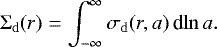
3.2 Column densities

We define the column density as the mass per 3-dim volume, density ρ, vertically integrated over the height z of the disk, 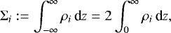$Σ_{i} : = \int_{- \infty}^{\infty} ρ_{i} d z = 2 \int_{0}^{\infty} ρ_{i} d z,$ $\begin{align*} \Sigma_i:=\int_{-\infty}^{\infty}\rho_i\,\textrm{d}{z}=2\int_{0}^{\infty}\rho_i\,\textrm{d}{z,} \end{align*}$ (14)

where i = {d, g, p} can be dust (d), gas (g), and planetesimals (p). We use Σ_d as the column density, including all solid particles without planetesimals. When it has St as an argument, it is the column density of particles with this Stokes number. Following Birnstiel et al. (2010), we define the dust column density distribution per logarithmic bin of grain radius a as 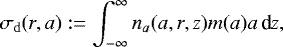$σ_{d} (r, a) : = \int_{- \infty}^{\infty} n_{a} (a, r, z) m (a) a d z,$ $\begin{align*} \sigma_{\mathrm{d}}(r,{a}):=\int_{-\infty}^{\infty}{n_{{a}}}({a},r,z){m}({a}){a}\,\textrm{d}{z}, \end{align*}$ (15)

where n_a is the number density per grain size bin. In this way, knowledge of the used size grid is not required and the total dust column density is given by $Σ_{d} (r) = \int_{- \infty}^{\infty} σ_{d} (r, a) d \ln a .$ $\begin{align*} {\Sigma_{\mathrm{d}}}(r)=\int_{-\infty}^{\infty}\sigma_{\mathrm{d}}(r,{a})\,\textrm{d}{\ln{{a}}}. \end{align*}$ (16)

As initial condition for the gas, we use the self-similar profile (Lynden-Bell & Pringle 1974) $Σ_{g} (r) = \frac{(2 - γ) M_{disk}}{2 π r_{c}^{2} (1 + Z_{0})} {(\frac{r}{r_{c}})}^{- γ} \exp [- {(\frac{r}{r_{c}})}^{2 - γ}],$ $\begin{equation*}{\Sigma_{\mathrm{g}}}(r)=\frac{(2-{\gamma}){M_{\mathrm{disk}}}}{2\pi{{r_{\mathrm{c}}}}^2(1+\dtog_0)}\left(\frac{r}{{{r_{\mathrm{c}}}}}\right)^{-{\gamma}}\exp{\left[-\left(\frac{r}{{{r_{\mathrm{c}}}}}\right)^{2-{\gamma}}\right]}, \end{equation*}$ (17)

where Z₀ = Σ_d∕Σ_g is the initial solid-to-gas ratio in terms of column densities. The initial dust column density is then given by Z₀ Σ_g(t₀).

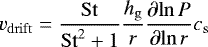
3.3 Drift velocities

From tiny dust grains up to boulders, particles are embedded in the gas disk. With the force of gravity from the central star balanced by the centrifugal force, particles move on Keplerian orbits. The action of the gas pressure gradient on the particles can be neglected because the internal density of the particles is so much higher than the gas density. The gas is subject to gravity, centrifugal force, and the pressuregradient force. When these forces balance each other, the gas moves on slightly sub-Keplerian orbits. Particles with St ≲ 1 are coupled to the gas, thus they are subject to a centrifugal deficiency as a result of sub-Keplerian gas motion and drift radially inward. As long as St < 1, this leads to a stronger radial drift for increasing St. When the particle Stokes number is larger than unity, they decouple from the gas and are subject to a headwind from the surrounding gas. The mass-to-surface ratio increases with size, and this effect becomes weaker for increasing St (i.e., increasing stopping time τ_s). The steady-state solution for radial drift reads (Nakagawa et al. 1986) $v_{drift} = \frac{St}{{St}^{2} + {(1 + ρ_{d} / ρ_{g})}^{2}} \frac{h_{g}}{r} \frac{\partial \ln P}{\partial \ln r} c_{s},$ $\begin{align*}{v_{\mathrm{drift}}}=\frac{{\mathrm{St}}}{{\mathrm{St}}^2+(1+{ \mdens_{\mathrm{d}} }/{\mdens_{\mathrm{g}}} )^2}\frac{{h_{\mathrm{g}}}}{r}{\dfrac{\partial{\ln{{P}}}}{\partial {\ln{r}}}}{c_{\mathrm{s}}}, \end{align*}$ (18)

which reduces to $v_{drift} = \frac{St}{{St}^{2} + 1} \frac{h_{g}}{r} \frac{\partial \ln P}{\partial \ln r} c_{s}$ $\begin{align*}{v_{\mathrm{drift}}}=\frac{{\mathrm{St}}}{{\mathrm{St}}^2+1}\frac{{h_{\mathrm{g}}}}{r}{\dfrac{\partial{\ln{{P}}}}{\partial {\ln{r}}}}{c_{\mathrm{s}}} \end{align*}$ (19)

for low dust-to-gas ratios (Weidenschilling 1977b). We use the latter expression for this paper to save computation time.

3.4 Planetesimal formation rate

For the planetesimal formation rate, we follow Lenz et al. (2019). The model is based on the idea that pebble traps appear and disappear on a given timescale. In those pebble traps, pebble clouds can then collapse to planetesimals.

In this model, the pebble flux (in mass per time) 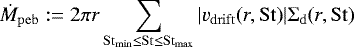${\dot{M}}_{peb} : = 2 π r \sum_{{St}_{min} \leq St \leq {St}_{max}} | v_{drift} (r, St) | Σ_{d} (r, St)$ $\begin{align*}{\dot{M}_{\mathrm{peb}}}:=2\pi r\sum_{{\stokes_{\mathrm{min}}}\leq{\mathrm{St}}\leq{\stokes_{\mathrm{max}}}}\vert{{v_{\mathrm{drift}}}(r,{\mathrm{St}})}\vert{\Sigma_{\mathrm{d}}}(r,{\mathrm{St}}) \end{align*}$ (20)

is transformed into planetesimals over a conversion length ℓ: 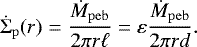${\dot{Σ}}_{p} (r) = \frac{{\dot{M}}_{peb}}{2 π r l} = ε \frac{{\dot{M}}_{peb}}{2 π r d} .$ $\begin{align*}{\dot{\Sigma}_{\mathrm{p}}}(r)=\frac{{\dot{M}_{\mathrm{peb}}}}{2\pi r\ell}={\varepsilon}\frac{{\dot{M}_{\mathrm{peb}}}}{2\pi r{d}}. \end{align*}$ (21)

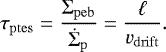
We assume that this conversion length is proportional to the gas pressure scale height h_g. Mass conversion from pebbles into planetesimals according to this recipe is only allowed if the condition 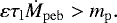$ε τ_{l} {\dot{M}}_{peb} > m_{p} .$ $\begin{align*}{\varepsilon}{\tau_{\mathrm{l}}}{\dot{M}_{\mathrm{peb}}}>{m_{\mathrm{p}}}. \end{align*}$ (22)

is fulfilled, where m_p is the mass of a single 100 km planetesimal and τ_l is the lifetime of traps. In this paper, we assume that τ_l = 100 t_orb for all simulations. ε is the efficiency with which pebbles are transformed into planetesimals. For more details, we refer to Lenz et al. (2019). With the help of the mean radial trap separation d, we can relate this parameter to the conversion length, ℓ = d∕ε. The jump from pebble size to objects 100 km in diameter is a direct result of the particle diffusion timescale within the particle cloud and the collapse timescale (Klahr & Schreiber 2015; Schreiber 2018; Gerbig et al. 2020).

3.5 Comparison to other planetesimal formation rate models

The model for the planetesimal formation rate from Lenz et al. (2019) differs from other models. Lenz et al. (2019) regulated planetesimal formation by a conversion length scale over which drifting particles were converted into planetesimals. The conversion length scale depends on the radial density of pebble traps and the efficiency of concentrating particles and converting pebble clouds into bound objects. Drążkowska et al. (2016) and Schoonenberg et al. (2018) suggested models for which planetesimal formation occurs with a certain efficiency per orbit from the local particle density. These models assume that particles are not trapped while drifting. Potentially, an equivalent situation might be reached for explicit traps that build up and vanish on a given timescale everywhere in the disk, with some average radial distance between each other. Lenz et al. (2019) parameterized this by the conversion length ℓ, see Eq. (3) in their paper.

Adding a gas gap to the simulation, Stammler et al. (2019) used the model of Schoonenberg et al. (2018) to produce planetesimals just outside this gap. The authors were able to reproduce the observed optical depth of HD 163296.

Eriksson et al. (2020) used the criterion from Yang et al. (2017) and assumed that all the available local mass is transformed into planetesimals when the condition is met for which particles in the midplane can concentrate in a particle-to-gas mass ratios of more than 10. For further discussion of other planetesimal formation models, see Lenz et al. (2019).

3.6 Advection-diffusion equation

The particle diffusion coefficient D_d for species i can be estimated with help of the gas diffusion coefficient $D_{g} = α_{t} c_{s} h_{g}$ $\begin{align*}{D_{\mathrm{g}}}={\alpha_{\mathrm{t}}}{c_{\mathrm{s}}}{h_{\mathrm{g}}} \end{align*}$ (23)

as (Youdin & Lithwick 2007) $D_{d}^{i} = \frac{D_{g}}{1 + {St}_{i}^{2}} .$ $\begin{align*} {D_{\mathrm{d}}}^i=\frac{{D_{\mathrm{g}}}}{1+\stokes_i^2}. \end{align*}$ (24)

This means that small particles are diffused with the gas and larger particles are less affected by gas diffusion. As first described by Fick (1855) and reviewed in more modern notation by Tyrrell (1964, his Eq. (1)), and derived from fundamental principles by Reeks (1983, his Eq. (25))² the diffusiveflux is given by $J_{diff}^{i} = - D_{d}^{i} \nabla ρ_{d}^{i}$ $\begin{align*}\boldsymbol{J}_{\mathrm{diff}}^i = -{D_{\mathrm{d}}}^i\nabla{ \mdens_{\mathrm{d}} }^i \end{align*}$ (25)

(see also Cuzzi et al. 1993), which gives the z-integrated version in radial direction, $j_{diff, r}^{i} = - \int_{- \infty}^{\infty} D_{d}^{i} \frac{\partial ρ_{d}^{i}}{\partial r} d z \approx - D_{d}^{i} \frac{\partial Σ_{d}^{i}}{\partial r} .$ $\begin{align*}j_{\mathrm{diff,r}}^i = -\int_{-\infty}^{\infty}{D_{\mathrm{d}}}^i{\frac{\partial {{ \mdens_{\mathrm{d}} }^i}}{\partial {r}}}\textrm{d}{z} \approx -{D_{\mathrm{d}}}^i{\frac{\partial{{\Sigma_{\mathrm{d}}}^i}}{\partial{r}}}. \end{align*}$ (26)

In the last step we used the fact that because of the Gaussian shape of $ρ_{d}^{i}$ ${ \mdens_{\mathrm{d}} }^i$ in z-direction, the highest contribution of the integral comes from the region within $[- h_{d}^{i}, h_{d}^{i}]$ $[-{h_{\mathrm{d}}}^i,{h_{\mathrm{d}}}^i]$ , within which the gas density does not change by much (especially because $h_{d}^{i} < h_{g}$ ${h_{\mathrm{d}}}^i<{h_{\mathrm{g}}}$ ). When the gas density is roughly constant, the particle Stokes number also remains roughly constant. When at $z = h_{d}^{i}$ $z={h_{\mathrm{d}}}^i$ the temperature is similar to the temperature of the midplane, $D_{d}^{i}$ ${D_{\mathrm{d}}}^i$ can be considered to be z-independent. As long as these conditions are met, the right-hand side of Eq. (26) gives a good approximation. Because particles exhibit diffusive mixing as a result of turbulent gas motion, they are not able to move faster than the turbulent gas motion driving it. This maximum diffusion speed can be estimated to be (Cuzzi et al. 2001) $v_{max} ≃ \sqrt{α_{t}} c_{s} .$ $\begin{align*} v_{\mathrm{max}}\simeq\sqrt{{\alpha_{\mathrm{t}}}}{c_{\mathrm{s}}}. \end{align*}$ (27)

We would like to point out that in the expressions in Desch et al. (2017), for instance, which are based on Morfill & Völk (1984), the diffusive flux is not given by $j_{diff, r}^{i} \neq - D_{d}^{i} Σ_{g} \frac{\partial}{\partial r} (\frac{Σ_{d}^{i}}{Σ_{g}}) .$ $\begin{align*} j_{\mathrm{diff,r}}^i \neq -{D_{\mathrm{d}}}^i{\Sigma_{\mathrm{g}}}{\frac{\partial{}}{\partial{r}}} \left(\frac{{\Sigma_{\mathrm{d}}}^i}{{\Sigma_{\mathrm{g}}}}\right). \end{align*}$ (28)

This expression is strictly speaking only valid for small particles, which couple to the gas motion on timescales shorter than the correlation time of the fastest turbulent eddy τ_Kolmogorov, that is, the smallest eddy at the dissipation scale of turbulence (Kolmogorov scale) τ_s < τ_Kolmogorov, or for constant gas densities. Otherwise, Eq. (26) should be used. Unfortunately, we do not know the value of τ_Kolmogorov. For further details on the different turbulence regimes, see, for example, Ormel & Cuzzi (2007). The difference between the two diffusion terms can be significant when the gas density drops quickly, as is the case for gap opening due to photoevaporation. Although Dubrulle et al. (1995) used this diffusive flux for the vertical direction (z derivative instead of r derivative), their result for the particle scale height is still valid because the gas density does not change much in the vertical direction within one particle scale height. By making use of Eq. (26), the advection-diffusion equation reads $\begin{array}{l} \frac{\partial Σ_{d}^{i}}{\partial t} + \frac{1}{r} \frac{\partial}{\partial r} {r [Σ_{d}^{i} v_{r}^{i} - D_{d, eff}^{i} \frac{\partial Σ_{d}^{i}}{\partial r}]} \\ = - \frac{f_{St} ε}{d} | v_{drift}^{i} | Σ_{d}^{i} \cdot θ ({\dot{M}}_{peb} - {\dot{M}}_{cr}) . \end{array}$ $\begin{align*} &{\frac{\partial{{\Sigma_{\mathrm{d}}}^i}}{\partial{t}}} +\frac{1}{r}{\frac{\partial{}}{\partial{r}}} \left\{ r\left[ {\Sigma_{\mathrm{d}}}^i{v_{\mathrm{r}}}^i-{D_{\mathrm{d,eff}}}^i{\frac{\partial{{\Sigma_{\mathrm{d}}}^i}}{\partial{r}}} \right] \right\} \nonumber\\ &\quad\ =-\frac{f_{{\mathrm{St}}}{\varepsilon}}{{d}}\vert{{v_{\mathrm{drift}}}^i}\vert{\Sigma_{\mathrm{d}}}^i \cdot\theta({\dot{M}_{\mathrm{peb}}}-{\dot{M}_{\mathrm{cr}}}) . \end{align*}$ (29)

Here, θ(⋅) is the Heaviside function, and ${\dot{M}}_{cr} : = \frac{m_{p}}{ε τ_{l}}$ $\begin{align*} {\dot{M}_{\mathrm{cr}}}:=\frac{{m_{\mathrm{p}}}}{{\varepsilon}{\tau_{\mathrm{l}}}} \end{align*}$ (30)

is the critical pebble flux required to allow planetesimal formation (Lenz et al. 2019). We introduce a smoothing function for the Stokes number dependency of the efficiency parameter ε, $\begin{array}{l} f_{St} = & {[\exp (- 12 \cdot (\lg (St) - \lg ({St}_{min} / 2))) + 1] \\ \times {[\exp (12 \cdot (\lg (St) - \lg (2 {St}_{max}))) + 1]}}^{- 1} . \end{array}$ $\begin{align*}f_{{\mathrm{St}}}=&\,\left\{\left[\exp{\left(-12\cdot\left(\lg{({\mathrm{St}})}-\lg{({\stokes_{\mathrm{min}}}/2)}\right)\right)}+1\right]\right. \nonumber\\ &\times\,\left.\left[\exp{\left(12\cdot\left(\lg{({\mathrm{St}})}-\lg{(2{\stokes_{\mathrm{max}}})}\right)\right)}+1\right]\right\}^{-1}. \end{align*}$ (31)

This prefactor is displayed in Fig. 3. The idea is to smooth out the strong dependence on the fragmentation speed; this is similar to the idea presented in Windmark et al. (2012), where particles have a velocity distribution.

The evolution of the gas is given by (Pringle 1981) $\frac{\partial Σ_{g}}{\partial t} = \frac{3}{r} \frac{\partial}{\partial r} [r^{1 / 2} \frac{\partial}{\partial r} (ν Σ_{g} r^{1 / 2})] + {\dot{Σ}}_{w},$ $\begin{align*}{\frac{\partial{{\Sigma_{\mathrm{g}}}}}{\partial{t}}} =\frac{3}{r}{\frac{\partial{}}{\partial{r}}} \left[ r^{1/2}{\frac{\partial{}}{\partial{r}}} \left( \nu{\Sigma_{\mathrm{g}}} r^{1/2} \right) \right]+\dot{\Sigma}_{\mathrm{w}}, \end{align*}$ (32)

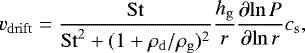
where ${\dot{Σ}}_{w}$ $\dot{\Sigma}_{\mathrm{w}}$ is a loss term due to photoevaporative winds. The photoevaporation model is based on Picogna et al. (2019) and described in Appendix A. For the viscosity ν we choose the turbulent viscosity according to Shakura & Sunyaev (1973), which is the same expression as Eq. (23).

Fig. 3

Illustration of Eq. (31) for St_min = 0.01 and St_max = 10.

3.7 Temperature model

In order to calculate the midplane gas temperature, we need the contribution from radiation (internal and external) as well as from accretion heating. From pure radiation heating (e.g., Armitage 2010) we obtain $T_{rad} = {(\frac{L_{⋆}}{4 π σ_{SB} r^{2}} θ + T_{bg}^{4})}^{1 / 4},$ $\begin{align*}T_{\mathrm{rad}}=\left(\frac{{L_{\star}}}{4\pi{\sigma_{\mathrm{SB}}} r^2}\theta+{T_{\mathrm{bg}}}^4\right)^{1/4}, \end{align*}$ (33)

where θ ≈ tanθ ≈ h_g∕r ≈ 0.04 (e.g., Chiang & Goldreich 1997; Pfeil & Klahr 2019). We set the background temperature due to external sources to T_bg = 10 K.

Gough (1981) described the luminosity evolution of the Sun as $L_{⋆} (t) = \frac{L_{⊙}}{1 + 2 / 5 \cdot (1 - t / t_{⊙})} .$ $\begin{align*} {L_{\star}}(t)=\frac{{L_{\odot}}}{1+2/5\cdot(1-t/t_{\odot})}. \end{align*}$ (34)

As the age of the Sun is approximately t_⊙≈ 4.6 × 10⁹ yr and our simulations run for a few 10⁶ yr, we can make the approximation $L_{⋆} \approx 5 L_{⊙} / 7 \approx 2.73 \times 10^{33} erg s^{-1} .$ $\begin{align*}{L_{\star}}\approx5L_{\odot}/7\approx2.73\times10^{33}\,\mathrm{erg\,s^{-1}}.\end{align*}$

For pure accretion heating (i.e., ignoring radiation heating for the moment), and without taking optical depth effects into account and assuming that $T_{acc} \propto c_{s}^{2}$ $T_{\mathrm{acc}}\propto{c_{\mathrm{s}}}^2$ , the local midplane temperature can be calculated as (Nakamoto & Nakagawa 1994; Pringle 1981) $T_{acc} = {(α_{t} Σ_{g} Ω \frac{9 k_{B}}{8 m_{g} σ_{SB}})}^{1 / 3} .$ $\begin{align*} T_{\mathrm{acc}}=\left({\alpha_{\mathrm{t}}}{\Sigma_{\mathrm{g}}}{\Omega}\frac{9{\mathrm{k_B}}}{8 {m_{\mathrm{g}}}{\sigma_{\mathrm{SB}}}}\right)^{1/3}. \end{align*}$ (35)

Following Ostriker (1963) and Armitage (2010, his Eq. (3.37)), we approximate the midplane temperature due to accretion and radiation heating as $T = {[(\frac{3}{4} τ_{R} + 1) T_{acc}^{4} + T_{rad}^{4}]}^{1 / 4} .$ $\begin{align*} T=\left[\left(\frac{3}{4}{\tau_{\mathrm{R}}}+1\right) T_{\mathrm{acc}}^4+T_{\mathrm{rad}}^4\right]^{1/4}. \end{align*}$ (36)

The Rosseland optical depth τ is approximated by $τ_{R} \approx κ_{R} \frac{1}{2} Σ_{d},$ $\begin{align*} \optdepth_{\mathrm{R}}\approx\kappa_{\mathrm{R}}\frac{1}{2}{\Sigma_{\mathrm{d}}}, \end{align*}$ (37)

where κ_R is the size- and wavelength-averaged Rosseland opacity (Birnstiel et al. 2018) that is calculated at every time step based on the local size distribution,and Σ_d is the column density of all particles except for planetesimals. We use this accretion heating model only for some further test cases. For the majority of the simulations presented in the main text, we used radiation heating alone, see Eq. (33).

3.8 Analyzed parameters

For the total disk masses we used values between the MMSN (0.013 M_⊙) and approximately the critical value at which disk fragmentation can occur, ~ 0.1 M_⊙ (Toomre 1964; Goldreich & Lynden-Bell 1965). However, for collapse due to the gravity of the disks themselves, the cooling time is also an important criterion (Baehr et al. 2017).

The disk size, which is approximately given by the characteristic radius r_c of our initial condition, spans from 10 to 100 au, based on observations (Andrews et al. 2010). For the viscosity power-law index γ we also allowed extreme cases, that is, 0.5 ≤ γ ≤ 1.5, and made the turbulence parameter disk radius dependent for the cases γ≠ 1, $α_{t} = α_{0} {(\frac{r}{r_{c}})}^{g},$ $\begin{align*} {\alpha_{\mathrm{t}}} = \alpha_0 \left( \frac{r}{{{r_{\mathrm{c}}}}} \right)^g, \end{align*}$ (38)

where g = γ + q − 3∕2 and T ∝ r^−q.

For the fragmentation speed, Musiolik & Wurm (2019) recently indicated that the value should be about 1 m s⁻¹. We still analyzed values up to the former default of 10 m s⁻¹.

Values for the solar metallicity span from Z = 1.34% (Asplund et al. 2009) to Z = 2% (for a review, see Vagnozzi 2019). We used Z = 0.0134 as our fiducial initial dust-to-gas ratio.

For the trap formation time τ_f, we took typical timescales for the significant evolution of disk instabilities such as the convective overstability, vertical convective instability, subcritical baroclinic instability, or vertical shear instability (Pfeil & Klahr 2019), as well as Hall magnetohydrodynamics (Bai & Stone 2014; Béthune et al. 2016). The values can span from a few hundred to some thousands of orbits, depending on how fast the instability evolves and how fast it can then create pressure bumps. Therefore we also considered the viscous timescale $τ_{visc} ~ \frac{1}{α_{t} Ω} = \frac{t_{orb}}{2 π α_{t}}$ $\begin{align*} \tau_{\mathrm{visc}}\sim\frac{1}{{\alpha_{\mathrm{t}}}{\Omega}}=\frac{{t_{\mathrm{orb}}}}{2\pi{\alpha_{\mathrm{t}}}} \end{align*}$ (39)

(e.g., Armitage 2010) on which structures could form. For example, for α_t ~ 10⁻⁴, this would give ~1600t_orb.

We studied turbulence levels that represent an almost laminar case (α_t = 10⁻⁵) up to a very turbulent state (α_t = 10⁻²). For the planetesimal formation efficiency, here defined as ε = 5h_g∕ℓ, we relied onnumerical experiments in order to judge whether values are high or low. We found that ε = 0.3 is already high, with almost all the mass that was originially in dust being in planetesimals by the end of the simulations, see Fig. 4. When this ratio is about 0.1, we consider the efficiency to be rather low, which is the case for ε ≈ 0.01.

X-ray luminosities are found in the range (Güdel et al. 1997; Vidotto et al. 2014) $10^{28} ≲ L_{X} / (erg s^{-1}) ≲ 10^{31} .$ $\begin{align*} 10^{28}\lesssim L_{\mathrm{X}}/(\mathrm{erg\,s^{-1}})\lesssim10^{31}. \end{align*}$ (40)

Table 1 summarizes all the different parameters that we determined for this paper.

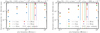Fig. 4

Final mass in planetesimals within a given disk radius shown in the legend, normalized to the initial total disk dust mass, as a function of planetesimal formation efficiency. Defining ε = 5h_g ∕ℓ, where ℓ is theconversion length over which pebbles are transformed into planetesimals. The vertical dashed lines show the predicted maximum at the outer edge of the respective zone. This means that the dashed blue line shows the predicted maximum at 1 au and the purple line shows this at 50 au. This plot shows ε variations from the first fiducial run (gray values in Table 1) in the left panel and from the second fiducial run in the right panel (bold values in Table 1).

Table 1

Parameters used in this study.

4 Results

4.1 Effect of planetesimal formation efficiency

Before analyzing the results of all nine different disk parameters, we would first like to concentrate on the planetesimal formation efficiency. Because many processes that we do not yet fully understand are hidden in this parameter, we first have to clarify which values are low or high. In the left panel of Fig. 4 we show for the first fiducial parameter set the final mass in planetesimals within a given disk region over the total initial dust mass as a function of planetesimal formation efficiency. All simulations were stopped at 10 Myr, or when essentially all the gas was drained. A linear regime for small ε is visible, which is expected because the formation rate scales linearly with this parameter (Eq. (21)). For very high efficiency values, the mass in all the regions should reach a plateau because the planetesimal profile is expected to lie very close to the initial condition of the dust. For an extreme case, the conversion length is infinitaly small and pebbles are all instantly transformed into planetesimals. When a critical high value of ε∕d is reached, the initial structure is basically reproduced, which leads to a plateau in this plot. Given these extreme cases, we expect there to be a sweet spot, that is, for a given efficiency, the final planetesimal mass reaches a local maximum. This behavior can be described by looking at timescales. How fast planetesimals can be built locally from pebbles is determined by the planetesimal formation timescale $τ_{ptes} = \frac{Σ_{peb}}{{\dot{Σ}}_{p}} = \frac{l}{v_{drift}} .$ $\begin{align*} {\tau_{\mathrm{ptes}}} = \frac{{\Sigma_{\mathrm{peb}}}}{{\dot{\Sigma}_{\mathrm{p}}}}=\frac{\ell}{{v_{\mathrm{drift}}}}.\vspace*{-3pt} \end{align*}$ (41)

At the sametime, pebbles are removed from their location by radial drift on the drift timescale $τ_{dr} = \frac{r}{v_{drift}} .$ $\begin{align*} {\tau_{\mathrm{dr}}} = \frac{r}{{v_{\mathrm{drift}}}}.\vspace*{-3pt} \end{align*}$ (42)

When τ_ptes < τ_dr, pebbles are transformed into planetesimals faster than particles are removed from their location by radial drift, that is, the planetesimal profile becomes closer to the initial dust profile. Setting these timescales equal and making use of ℓ = ε∕d, we obtain $ε = \frac{d}{r},$ $\begin{align*}{\varepsilon} = \frac{{d}}{r},\vspace*{-3pt} \end{align*}$ (43)

which means that for a fixed location in the disk, only the gas temperature matters because 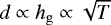$d \propto h_{g} \propto \sqrt{T}$ ${d}\propto{h_{\mathrm{g}}}\propto \sqrt{T}$ . Starting from very low ε, the mass increases linearly until the sweet spot, where planetesimal formation and drift occur on similar timescales. When ε is increased even more, pebbles are transformed into planetesimals before they can significantly drift, leading to a profile that is closer to the initial dust profile the higher ε.

However, considering the simplicity of the estimate for the maximum, the prediction works surprisingly well for both parameter sets (compare the left and right panels of Fig. 4). The difference in the shape of the curves may be related to whether the disk is mostly limited by drift or fragmentation, as well as by the mass budget in pebbles. For the fragmentation-limited case, material remains longer within a certain region in the disk because fragmentation events force it to start growing again from tiny, very slowly drifting dust grains, or small dust that is swept up by larger grains. Figure 5 shows that the high fragmentation speed in the first parameter set allows the disk to be mostly fragmentation limited in the inner disk and drift limited in the outer disk over the typical time span of planetesimal formation. However, for the second parameter set, the fragmentation speed is so low that during the time of planetesimal formation, basically the entire disk is fragmentation limited. Also compare to the findings of Birnstiel et al. (2012), which did not include planetesimal formation.

The vertical purple lines in Fig. 4 mark the point beyond which all the initial dust mass is bound in planetesimals because there is not much planetesimal mass outside of 50 au and because this is a prediction for the maximum in mass at 50 au. For the radial positions farther in, the required planetesimal formation efficiency to reach a maximum in mass is even lower.

4.2 Deeper analysis of special cases

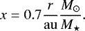
In this section we focus on the two fiducial runs and on the most appropriate simulation, where only the latter contains a simple model for accretion heating that we described in Sect. 3.7. Figure 6 shows the time evolution of the gas, dust, and planetesimal profiles (top panels) as well as the local values of these at three different disk radii (bottom panels). The kinks in the planetesimal profiles (solid lines) and dust profiles (dotted lines) inidcate the position of the water-ice line in that simulation. Interior to the water-ice line, loss of water ice due to sublimation is assumed. Figure 6 compares both fiducial runs (see the gray and bold values in Table 1), which are different from each other in two main aspects. For the first fiducial run we used a turbulence strength parameter of α_t = 10⁻³ and a fragmentation speed of v_f = 10 m s⁻¹, whereas for the second fiducial run we set α_t = 10⁻⁴ and v_f = 1 m s⁻¹. Although for the latter case both values are one order of magnitude lower than in the former, the smaller v_f in the second fiducial run leads to much smaller maximum particle sizes because the fragmentation barrier scales quadratically with v_f but only inversely linearly with α_t (Birnstiel et al. 2012). As a result, almost the entire disk is limited by fragmentation over most of the time of planetesimal formation in the second parameter set, while the first becomes drift limited much faster (see Fig. 5). Figure 6 also shows that higher α_t causes the disk to spread faster, with material being removed in the very outer regions due to the constant external far-UV sink term that we used.

Figure 5 shows the particle flux for particles of different sizes in the Stokes number space as a function of disk radius at three different snapshots. The fragmentation (red lines) and drift limit (purple lines) set the maximum size of the flux-dominating particle species. The horizontal gray line marks the Stokes number beyond which particles are assumed to contribute to particle trapping and planetesimal formation, see also Fig. 3. Within ~ 3 au, some particles have higher Stokes numbers, forming a kink feature because they enter the Stokes drag regime (see Figs. 5 and B.3). However, it looks much less extreme in the grain size space. More details on the special case including accretion heating can be found in Appendix B, where we show the time evolution of the pebble flux and of the planetesimal, dust, and gas profiles.

4.3 Mass evolution

It might be valuable to know if and when the total mass in planetesimals saturates. This saturated mass can be compared with the MMSN solid mass. When this mass is not reached, we consider the parameter set of that simulation to be unable to reproduce the Solar System, as usually several times the MMSN is needed in order to obtain results that are comparable to the Solar System. Figures 7 and 8 show the time evolution in mass of the first and second sample, respectively. In each panel, only one parameter was changed compared to the ficucial parameter set shown in the header of both figures. The final value of the total disk mass that is in planetesimals can be compared to the minimum mass for the solar nebula based on Weidenschilling (1977a) and Hayashi (1981). The required mass for initial planetesimals is marked by gray regions. When the final mass is below the gray region for a given parameter set, this set can be excluded for the solar nebula. In both figures, initial dust-to-gas ratios of 0.003 and lower are not able to lead to the MMSN mass in planetesimals. A fragmentation speed of v_f = 10² cm s⁻¹ seems to be a critical value below which the MMSN mass cannot be reached unless the initial dust-to-gas ratio Z₀ > 0.0134, the turbulence strength α_t ≤ 10⁻⁴ (here this parameter is also used for vertical and radial particle diffusion, as well as relative turbulent velocities), or ε > 0.03. For a disk starting with M_disk < 0.1 M_⊙, ε or Z₀ might need even higher values to reach a final planetesimal disk mass more massive than the MMSN.

The yellow line in the middle lower panel of Fig. 8 shows a case of low planetesimal formation efficiencies in a mostly fragmentation-limited disk. In this case, after about 10⁵ yr, photoevaporation allows another phase of planetesimal formation after the planetesimal mass in the disk reached a plateau. The same effect is detected for high initial dust-to-gas ratios, see the case of Z = 0.03 in the center panel of Fig. 8. In both cases the reason for the second planetesimal formation phase is the higher mass budget. For low ε, particles survive longer in a fragmentation-limited disk because their average radial drift velocity is much lower as a result of disruptive collisions that replenish slowly drifting dust grains, and less mass is transformed into planetesimals. For Z ≳ 0.03, the initial particle mass budget is already so high that there remains enough mass for planetesimal formation at later times, when photoevaoration has removed a significant amount of gas mass. However, this effect of a second planetesmial formation phase only occurs if the disk is mostly fragmentation limited, which applies for the results shown in Fig. 8 but not for those shown in Fig. 7, in which case the disks are mostly drift limited. Additionally, the second planetesimal formation phase induced by photoevaporation is not sufficient to reach the mass of the MMSN for low planetesimal formation efficiencies, that is, for ε ≲ 0.01.

The first sample, shown in Fig. 7, leads to higher masses of the planetesimal population than in the second sample, shown in Fig. 8. The reason for this is that in the first sample grains can grow to larger sizes because the fragmentation speed is higher. However, both samples used the parameterized planetesimal formation model of Lenz et al. (2019), see Sect. 3.4. Again, in this model, particle traps are only considered through parameters, but the gas profile is smooth, without pressure bumps or gaps, unless caused by photoevaporation. Pressure bumps in the gas profile would lead to a reduction in radial drift speed, allowing particles to remain longer in certain disk regions (e.g., Pinilla et al. 2012), even when these traps appear and disappear on a given timescale. This could lead to longer planetesimal formation and greater effect of photoevapotation. However, this might not change the results significantly and therefore leaves our conclusions untouched.

Fig. 5

Local particle flux in Earth masses per year resulting from pure radial drift per size bin (color) as a function of Stokes number and disk radius. Here, we show the first fiducial run in the left panels (gray values in Table 1) and the second fiducial run in the right panels (bold values in Table 1), both at three different snapshots. The orange (purple) line shows the fragmentation (drift) limit, and the gray line the threshold Stokes number that is required to participate in planetesimal formation (but see the smoothing function Eq. (31)). Particles in the region below the dashed white line have positive total radial velocities, i.e., they are moving outward. For the simulation shown in the left panels, outside of ~ 10 au the disk is limited by drift over most of the time of planetesimal formation. For the simulation shown in the right panels, the disk is mostly limited by fragmentation.

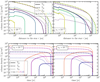Fig. 6

Top panels: planetesimal (solid), gas (dashed), and total dust (dotted) vertically integrated density profiles at different times. Bottom panels: same quantities, but as a function of time, for three different disk locations. Both fiducial simulations are compared, where the first (gray values in Table 1) is shown in the right and the second (bold valuesin Table 1) in the left panels.

4.4 Deep parameter analysis

The final planetesimal profiles for all nine parameters show a huge variety of possible parameters for the solar nebula. It is reassuring that the model works not only for a very finely tuned subset of parameter choices. Although the different parameters can influence each other, it is still possible to draw some conclusions. Table 2 shows the parameters that fail to fulfill the outer Solar System constraints or the MMSN mass. In Table 3 we present disk parameter ranges that might be able to reproduce the Solar System. These conclusions are based on Table 2. How much mass the initial disk should contain depends on the fragmentation speed because this determines how much mass is in particles with St ≳ 0.01.

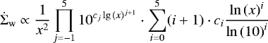
Our parameter analysis is based on Figs. 7–10. The last two of these figures show the column density profiles of the final planetesimal population. In each panel only one parameter is varied compared to the fiducial parameter set (dashed lines). In the background, the gray boxes represent the mass constraints discussed in Sect. 2.

The initial characteristic radius r_c has two main effects. One is the radial position beyond which the dust and gas density drops exponentially. The second is that for smaller (larger) r_c there is more mass in the inner (outer) disk region. When the disk is too large, there is simply too much mass available around 40 au and beyond to form planetesimals. Too much mass in the outer disk then leads to violation of the upper CCKBO constraint. Whether this constraint is indeed violated also depends on the initial disk mass, the planetesimal formation efficiency, the initial dust-to-gas ratio, and the viscosity power-law index γ. However, for a narrow set of these four parameters, it is possible to determine constraints for r_c.

The fragmentation speed v_f changes the outcome greatly because the fragmentation limit depends quadratically on this parameter. For v_f ≳ 10 m s⁻¹ γ ~ 0.5 is beneficial becaue of the stronger density drop in the outer disk; see the orange line in the top right panel of Fig. 9. However, for v_f ≳ 1 m s⁻¹, more than M_disk ≳ 0.1 M_⊙ is required to create enough mass to build all planets, specifically in the inner disk part (≲ 15 au); see the orange line in the top right panel of Fig. 10.

When v_f < 1 m s⁻¹, too few or no particles with St ≳ 0.01 would be formed, which is the necessary Stokes number to make trapping, and the collapse of pebble clouds into planetesimals work. With v_f = 1 m s⁻¹ it is already difficult to meet all the constraints, especially a total mass in planetesimals higher than the minimum mass solar nebula (Weidenschilling 1977a; Hayashi 1981); see the lowest line in the middle left panel of Fig. 7 and the dashed lines in Fig. 8.

The initial dust-to-gas ratio Z₀ determines how much mass is initially bound in particles, and it also determines the dust dynamics because a low dust-to-gas ratio leads to a drift-limited disk that quickly loses particles as a result of drift. Large Z₀ of up to approximately 0.03 seem to allow fulfilling the mass constraints on initial planetesimals. However, values of ≲ 0.003 lead to a mass in the final planetesimal population that is too low, as shown in Figs. 7–10.

The more time particles have to drift from the region outside of ~ 50 au to the inner parts before planetesimal formation, the better the CCKB constraints can be met. Alternatively, traps might not occur outside of 50 au at all (Pfeil & Klahr 2019). From the simulations we conclude that the trap formation time must be τ_f > 300 t_orb or even ≳ 1000 t_orb. Other values lead to masses between ~30 and 50 au, which are orders of magnitudes higher than the upper limit.

Constraining values for the turbulence parameter α_t is also linked to the fragmentation speed because the fragmentation limit scales inversely linear with α_t but quadratically with v_f. For this limit, only the relative velocity matters. However, we assumed that vertical and radial diffusion, as well as the viscosity parameter for the gas, have the same value α_t that we used for the turbulent velocities. For smaller α_t, particles can settle closer to the midplane. When this value is low enough, growth is not limited by relative turbulent velocties but by relative settling speeds or relative radial drift. When α_t is high (~ 10⁻²), relative turbulent velocities are too high to allow St > 0.01 particles. Atthe same time, the radial viscous gas motion drags dust along to the outer regions of the disk, leading to too much mass in planetesimals outside of 30 au. For v_f ~ 10 m s⁻¹ we therefore suggest α_t ~ 10⁻⁵−10⁻³, while the upper end should be up to a few 10⁻⁴ if v_f~ 1 m s⁻¹.

Values of ε∕d ≤ 0.002∕h_g can be excluded for the solar nebula (if ε and d∕h_g are constant), because the total final planetesimal mass in the disk is below the MMSN, and the mass required for the Nice disk cannot be reached. Unless the solar nebula was not very small (r_c ≲ 10 au), planetesimal formation should not have been too efficient, that is, ε∕d ≲ 0.06∕h_g. Otherwise, too many planetesimals are formed outside of 30 au. The range of possible values therefore is 0.002 < εh_g∕d ≲ 0.06.

Photoevaporation did not affect the final planetesimal profile significantly for small enough disks (r_c ≲ 20 au). However, for large disks (r_c ~ 100 au), it can make a difference. This case is not relevant for finding similar conditions to the solar nebula, however, because in this case, too much mass is bound in planetesimals in the outer disk regions in any case.

In the left panel of Fig. 4, the plateau is reached for lower values of ε∕d than in the right panel. This is linked to the lower pebble mass that is available for planetesimal formation because the lower fragmentation velocity leads to smaller maximum Stokes numbers.

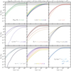Fig. 7

Total planetesimal mass as a function of time for the first sample (gray values in Table 1). The fiducial values for this set of simulations are shown in the header of the plot. In each panel, the simulation with those parameters is shown as the dashed gray line, and the solid lines with colors show simulation results where only one parameter of the set was changed. The gray area shows values more massive than the solids of the MMSN (Weidenschilling 1977a; Hayashi 1981).

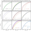Fig. 8

Same as Fig. 7, but for the second sample (variations to the bold values in Table 1). The fiducial run produces just enough planetesimal mass in the disk to reach the MMSN mass in solids, even though the disk mass already is at the high end. From this point of view, either a higher initial dust-to-gas ratio, a higher planetesimal formation efficiency, or a higher fragmentation speed are required. Bottom left panel: no line is visible for α_t = 0.01 as no planetesimals are formed in that case.

4.5 Effects of accretion heating on the results

Accretion heating leads to a hotter inner disk, which is good because not a single planetesimal was detected inside the orbit of Mercury. This means that the planetesimal profile has to drop drastically in the inner region before it reaches the current radial position of Mercury. This can be satisfied as a result of the higher gas temperatures because they force the fragmentation limit to be at lower Stokes numbers, and to a larger conversion length (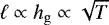 $l \propto h_{g} \propto \sqrt{T}$ $\ell\propto{h_{\mathrm{g}}}\propto\sqrt{T}$ ). In this simulation the ice line moves radially over time, therefore the profile shows no distinct kink feature. The constraints on the outer disk, that is, the Nice disk and the CCKB, are the strongest constraints we have. The other constraints may be slightly more flexible. These constraints are approximately met by this simulation.

Because the temperature model presented in this paper was not tested in a comprehensive way, for instance, by comparing it with modelsof Hubeny (1990) or Nakamoto & Nakagawa (1994), we only used it to show one special case. In addition, planetesimal–planetesimal collisions would replenish the small dust population (Gerbig et al. 2019). This effect is not taken into account in this paper but might change the gas midplane temperature through changes in the mean dust opacity.

We highlight one special case with parameters M_disk∕M_⊙ = 0.1, r_c ∕au = 20, γ = 1, v_f ∕cm s⁻¹ = 2 × 10², Z₀ = 0.0134, τ_f ∕t_orb = 1600, α_t = 3 × 10⁻⁴, ε = 0.05, and L_X ∕erg s⁻¹ = 3 × 10²⁹. We refer to this as the most appropriate simulation in this paper. The final planetesimal profile is shown in the top left panel of Fig. 10 as a dotted line.

Table 2

Parameters that can be excluded to reproduce the solar nebula based on Figs. 7, 8, 9, and 10.

Table 3

Parameter ranges that might work for reproducing the Solar System.

5 Summary

We used an extended version of the Lenz et al. (2019) model, including Stokes drag for particles, and allowed the gas to evolve viscously while photoevaporation removed gas over time. The analyzed parameter space was largely increased. While this paper provides a parameter study for pebble flux-regulated planetesimal formation, we focused on meeting Solar System constraints for initial planetesimals. Therefore we used two different default parameter sets and varied one out of nine parameters per simulation. While some parameters can be excluded, the model seems to be very robust overall, therefore it does not require parameter fine-tuning in order to fulfill the constraints.

The computation times of the simulations were between about a week and six months and were run on ten cores each. More than ten cores for one simulation would not decrease the computation time significantly because the code cannot make use of further parallelization. The runs of the second sample, in particular, were running for months. To shorten the computation time, a simple model must be used such as the two-population model presented by Birnstiel et al. (2012). However, this simplified model was only tested for a narrow set of parameters and causes deviations from DustPy simulations for certain parameters. Additionally, the two-population model was not yet tested in detail with the inclusion of the planetesimal formation model that was used in this study. A simple model that reproduces the results shown in this study is likely possible, but we preferred to use DustPy in order to rely on fundamental physics principles and a sophisticated growth and fragmentation model rather than simplified and untested models.

In Sect. 2 we suggested mass constraints for initial planetesimals in different regions of the disk:

0.7−1 au: 0.1−2.77 M_⊕
2−3 au: 0.002−5 M_⊕
4−15 au: 66−unknown M_⊕
15−30 au: 10−unknown M_⊕
30−50 au: 0.008−0.1 M_⊕

Within 0.7 au and outside of 50 au, there might have been nothing or a very low mass in planetesimals. These suggested constraints are illustrated in Figs. 1 and 2.

The fragmentation speed v_f that leads to breakup in particle collisions and the turbulence parameter of relative velocities α_t determine how large particles can grow. When the combination of both leads to a fragmentation limit that is close to Stokes numbers of 0.01, the available mass for planetesimal formation is affected by these parameters. A constraint in total initial disk mass therefore has to be linked to (mostly) v_f. To fulfill the constraints we suggested, we need M_disk ≳ 0.1 M_⊙ for v_f ~ 1 m s⁻¹ and M_disk ≳ 0.02 M_⊙ for v_f ≳ 10 m s⁻¹. In addition, the solar nebula was not larger than r_c ≲ 50 au (r_c is the initial transition radius between a power law and a dropping exponential profile). The power-law index of that inner region was likely about γ ~ 1, but for high fragmentation speeds, γ ~ 0.5 can be beneficial for the outer region because of the density drop (if traps can be formed outside of 50 au). To allow pebbles with St ≳ 10⁻² to form, which is approximately the Stokes number required for trapping and subsequent planetesimal formation, v_f ≳ 1 m s⁻¹ is required. For the initial dust-to-gas ratio, many values 0.01 ≲ Z₀ ≲ 0.03 might work, but Z₀ ≲ 0.003 leads to too little mass in planetesimals. Outside of 50 au, traps needed at least 300 t_orb or never formed there. For the turbulence parameter we find a wide range of possible values α_t ~ 10⁻⁵−10⁻³ (or only up to a few 10⁻⁴ if v_f ~ 1 m s⁻¹). Because disk parameters can affect each other, we also find a wide range for the radial pebble-to-planetesimal conversion length: 0.002 < h_g∕ℓ ≲ 0.06. If the disk is sufficiently small (r_c ≲ 20 au), photoevaporation does not change the final planetesimal profile by much. The parameters of our most appropriate case, which includes a simple accretion heating model, are the following: M_disk∕M_⊙ = 0.1, r_c ∕au = 20, γ = 1, v_f ∕cm s⁻¹ = 2 × 10², Z₀ = 0.0134, τ_f ∕t_orb = 1600, α_t = 3 × 10⁻⁴, and ε = 0.05, and L_X ∕erg s⁻¹ = 3 × 10²⁹ (see the dotted line in the top left panel of Fig. 10).

We estimated the maximum mass in planetesimals by equating the planetesimal formation and drift timescale. This approach leads to ℓ = r, see Eq. (43), which seems to fit our simulation results well (see Fig. 4). When the planetesimal formation timescale is much shorter than the drift timescale, the planetesimal profile reproduces the initial dust profile. Planetesimal formation efficiencies lower than the value corresponding to this sweet spot lead to planetesimal profiles steeper than the initial dust profile or even steeper than the minimum mass solar nebula profile. This effect has been observed in Lenz et al. (2019), and this study provides an estimate for the transition to more local planetesimal formation, which is linked to slopes closer to the initial dust profile.

Within the model, further limitations are that no pebble accretion was included, which might especially affect the planetesimal profile in the inner disk as pebbles are accreted before they reach this zone. In addition, our simulations did not consider planetesimal-planetesimal collisions, which would lead to multiple generations in planetesimals, pebbles, and dust.

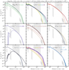Fig. 9

Final (at 10 Myr) planetesimal column density as a function of disk radius for the first sample (gray values in Table 1). The fiducialvalues for this set of simulations are shown in the header of the plot. In each panel, the simulation with those parameters is shown as dashed gray line, and the solid lines with colors show simulation results where only one parameter of the set was changed. The gray areas represent the constraints that we described in Sect. 2, where the mass in the given region was translated into a column density, assuming a planetesimal profile ∝ r^−2.25 (see Eq. (37) of Lenz et al. 2019). For the outermost region, we also overplotted a box ∝ r⁻⁸.

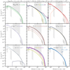Fig. 10

Same as Fig. 9, but for the second sample (variations to the bold values in Table 1). If ε is high enough, photoevaporation does not change the result significantly. It seems to have an effect for low ε, however; see the yellow line in the bottom middle panel of Fig. 8. Top left panel: we also plot the most appropriate case as a dotted line (last row in Table 1).

6 Conclusions

The MMSN is not consistent with viscous disk evolution models and does not provide enough mass in the giant-planet-forming region to allow strong gas accretion (see Fig. 2). While typically the MMSN distribution is assumed to be present from the beginning, the timing of substantial planetesimal formation could also matter for further embryo formation and evolution. We have shown that pebble flux-regulated planetesimal formation produces beneficial planetesimal distributions for a wide range of parameters, both with respect to planetesimal formation and initial conditions of the disk. Even though the effect of disk parameters on the evolution of initial planetesimals works both ways, some constraints on these parameters were found in this study. If we had worked with only a narrow set of parameters that could reproduce the Solar System, we would have had to fine-tune the model. This stresses the applicability of our parameterization to models of planet formation such as population synthesis models.

Acknowledgements

C.L. thanks Remo Burn, Thomas Pfeil, Oliver Völkel, Giovanni Picogna, Paola Pinilla, Christoph Mordasini, Alessandro Morbidelli, Andreas Schreiber, Bertram Bitsch, Joanna Drążkowska, Vincent Carpenter, Peter Rodenkich, Chris Ormel, Matthew Holman, Matias Garate, and Oliver Schib for helpful discussions. We would like to thank the referee KleomenisTsiganis for comments and suggestions on how to improve the readability and quality of the paper. This work was funded in parts by the Deutsche Forschungsgemeinschaft (DFG, German Research Foundation) as part of the Schwerpunktprogramm (SPP, Priority Program) SPP 1833 “Building a Habitable Earth”, priority program SPP 1992: “Exoplanet Diversity” under contract KL 1469/17-1, by the priority program SPP 1385 “The first ten million years of the Solar System” under contract KL1469/4-(1-3) “Gravoturbulent planetesimal formation in the early Solar System”. Futhermore DFG Research Unit FOR2544 “Blue Planets around Red Stars” under contract KL 1469/15-1. This research was also supported by the Munich Institute forAstro- and Particle Physics (MIAPP) of the DFG cluster of excellence “Origin and Structure of the Universe” and was performed in part at KITP Santa Barbara by the National Science Foundation under Grant No. NSF PHY11-25915.

Appendix A Photoevaporation

For the gas-loss rate due to photoevaporation, we followed Picogna et al. (2019) (X-ray and extreme UV). Carbon depletion can have significant effects (Wölfer et al. 2019) that we did not take into account. For the profile provided by Picogna et al. (2019) we used the scaling with stellar mass from Owen et al. (2012). The equations presented in this section are only for gas, but do not remove particles from the simulation. For the sake of brevity, we define $x = 0.7 \frac{r}{au} \frac{M_{⊙}}{M_{⋆}} .$ $\begin{align*} x = 0.7\frac{r}{{\mathrm{au}}}\frac{{M_{\odot}}}{{M_{\star}}}. \end{align*}$ (A.1)

The photoevaporation profile is given by ${\dot{Σ}}_{w} \propto \frac{1}{x^{2}} \prod_{j = - 1}^{5} 1 0^{c_{j} \lg {(x)}^{j + 1}} \cdot \sum_{i = 0}^{5} (i + 1) \cdot c_{i} \frac{\ln {(x)}^{i}}{\ln {(10)}^{i}}$ $\begin{align*} \dot{\Sigma}_{\mathrm{w}}\propto\frac{1}{x^2}\prod_{j=-1}^5 10^{c_j\lg{(x)^{j+1}}}\cdot\sum_{i=0}^5(i+1)\cdot c_i\frac{\ln{(x)}^i}{\ln{(10)}^i} \end{align*}$ (A.2)

with parameters $\begin{array}{l} c_{- 1} = - 2.8562 \\ c_{0} = 5.7248 \\ c_{1} = - 11.4721 \\ c_{2} = 16.3587 \\ c_{3} = - 12.1214 \\ c_{4} = 4.3130 \\ c_{5} = - 0.5885. \end{array}$ $\begin{align*} &c_{-1} = {-}\hphantom{1}\!\!2.8562 \nonumber\\ &c_0 = \hphantom{-1}5.7248 \nonumber\\ &c_1 = -11.4721 \nonumber\\ &c_2 = \hphantom{-}16.3587 \nonumber\\ &c_3 = -12.1214 \nonumber\\ &c_4 = \hphantom{-1}4.3130 \nonumber\\ &c_5 = {-}\hphantom{1}\!\!0.5885. \end{align*}$ (A.3)

The expression is normalized such that the total mass-loss rate ${\dot{M}}_{X} = \int_{0}^{\infty} 2 π r {\dot{Σ}}_{w} d r$ $\begin{align*} \dot{M}_{\mathrm{X}}=\int_0^{\infty}2\pi r\dot{\Sigma}_{\mathrm{w}}\textrm{d}{r} \end{align*}$ (A.4)

is given by $\begin{array}{l} \lg (\frac{{\dot{M}}_{X}}{M_{⊙} {yr}^{- 1}}) \\ = A_{L} \cdot \exp {\frac{1}{C_{L}} {[\ln (\lg (\frac{L_{X}}{erg s^{-1}})) - B_{L}]}^{2}} + D_{L}, \end{array}$ $\begin{align*} &\lg{\left(\frac{\dot{M}_{\mathrm{X}}}{{M_{\odot}}\,{\mathrm{yr}}^{-1}}\right)} \\ \nonumber &\quad\ = A_{\mathrm{L}}\cdot\exp{\left\{\frac{1}{C_{\mathrm{L}}}\left[\ln{\left(\lg{\left(\frac{L_{\mathrm{X}}}{\mathrm{erg\,s^{-1}}}\right)}\right)}-B_{\mathrm{L}}\right]^2\right\}}+D_{\mathrm{L}}, \end{align*}$ (A.5)

with parameters $\begin{array}{l} A_{L} = - 2.7326 \\ B_{L} = 3.3307 \\ C_{L} = - 2.9868 \times 10^{- 3} \\ D_{L} = - 7.2580. \end{array}$ $\begin{align*} &A_{\mathrm{L}} = -2.7326 \nonumber\\ &B_{\mathrm{L}} = \hphantom{-}3.3307 \nonumber\\ &C_{\mathrm{L}} = -2.9868\times10^{-3}\nonumber\\ &D_{\mathrm{L}} = -7.2580. \end{align*}$ (A.6)

Outside of 120 au × M_⋆∕(0.7M_⊙), we set ${\dot{Σ}}_{w} (r > 120 au \frac{M_{⋆}}{0.7 M_{⊙}}) = 3 \times 10^{- 15} g {cm}^{-2} s^{-1}$ $\begin{align*} \dot{\Sigma}_{\mathrm{w}}\left(r>120\,{\mathrm{au}}\frac{{M_{\star}}}{0.7{M_{\odot}}}\right)=3\,{\times}\,10^{-15}\,\mathrm{g\,cm^{-2}\,s^{-1}} \end{align*}$ (A.7)

due to external far-UV radiation.

For the case of an inner hole, we also follow Picogna et al. (2019). The hole radius r_h is implicitly defined by the radially integrated midplane gas number density, $\int_{0}^{r_{h}} \frac{Σ_{g}}{\sqrt{2 π} h_{g} m_{g}} d r = 10^{22} {cm}^{- 2} .$ $\begin{align*} \int_{0}^{r_{\mathrm{h}}}\frac{{\Sigma_{\mathrm{g}}}}{\sqrt{2\pi}{h_{\mathrm{g}}} {m_{\mathrm{g}}}}\textrm{d}{r}=10^{22}\,\mathrm{cm}^{-2}. \end{align*}$ (A.8)

The profile with inner hole becomes ${\dot{Σ}}_{w, h} \propto \frac{a_{h}}{2 π r / au} b_{h}^{δ x} δ x^{c_{h} - 1} [δ x \cdot \ln (b_{h}) + c_{h}],$ $\begin{align*} \dot{\Sigma}_{\mathrm{w,h}}\propto \frac{a_{\mathrm{h}}}{2\pi r/{\mathrm{au}}}b_{\mathrm{h}}^{\delta x}{\delta x}^{c_{\mathrm{h}}-1} \left[\delta x\cdot\ln{(b_{\mathrm{h}})+c_{\mathrm{h}}}\right], \end{align*}$ (A.9)

where δx = (r − r_h)∕au, and the parameters are given by $\begin{array}{l} a_{h} & = 0.11843, \\ b_{h} & = 0.99695, \\ c_{h} & = 0.48835. \end{array}$ $\begin{align*} \begin{aligned} a_{\mathrm{h}} &= 0.11843, \\ b_{\mathrm{h}} &= 0.99695, \\ c_{\mathrm{h}} &= 0.48835. \end{aligned} \end{align*}$ (A.10)

The gas-lossrate is normalized such that $1.12 {\dot{M}}_{X} = \int_{0}^{\infty} 2 π r {\dot{Σ}}_{w, h} d r .$ $\begin{align*} 1.12\dot{M}_{\mathrm{X}}=\int_0^{\infty}2\pi r\dot{\Sigma}_{\mathrm{w,h}}\textrm{d}{r}. \end{align*}$ (A.11)

Appendix B Most appropriate simulation that includes accretion heating

This appendix concentrates on a special case with accretion heating that is linked to the size distribution of solids. Figure B.1 shows the pebble flux as a function of disk radius at different snapshots and as a function of time at different disk radii. The interpretation of this figure is similar to the interpretation given in Lenz et al. (2019): when the critical flux for planetesimal formation is reached, the flux is orders of magnitude higher than the critical value Ṁ_cr (above the shaded areas in both panels). Photoevaporation (an effect not included in Lenz et al. 2019) leads to a small increase in pebble flux at late times; see the evolution after ~8 × 10⁶ yr in the lower panel of Fig. B.1. However, this increase has only a negligible effect on the final planetesimal population because the pebble flux has dropped by many orders of magnitude compared to its maximum value.

In Fig. B.2 the ice line radially moves over time because in this simulation, the gas temperaturedepends on dust evolution. The kink feature in planetesimals that is clearly visible at early times (~ 10⁴ yr) is therefore smeared out at late times (~10⁶ yr). At all threelocations shown in the bottom panel, planetesimal formation continues for ~ 10⁶ yr with significant mass contributions. A higher X-ray luminosity (up to ~10³⁰ erg s⁻¹) would not change the results by much as the disk would not vanish before ~ 2 Myr. At this time, the planetesimal population has already saturated.

For our most appropriate case, which includes accretion heating (Fig. B.3), the higher gas midplane temperatures in the inner disk region cause smaller maximum Stokes numbers than a situation with pure radiation heating. At late times (~ 1 Myr), enough dustwas converted into planetesimals, causing the opacity to drop, and the gas temperatures are therefore much lower than in the initial phase of disk evolution. As a result, higher Stokes numbers can be reached, and significantly more planetesimals are formed within ~1 au. This effect is also visible in Figs. B.1 and B.2.

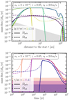Fig. B.1

Pebble flux in units of Earth masses per year for different times as a function of disk radius (upper panel) and as a function oftime for different disk locations (lower panel). Here, we show data from the accretion heating simulation (the most appropriate case, see the last row in Table 1). Solid lines show the pebble flux using the smoothing function Eq. (31), dashed lines show the total flux, i.e., taking all solid material into account, except for planetesimals. For the upper panels, sub-critical fluxes are marked by the gray zone. They are shown in the respective colors in thelower panels.

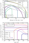Fig. B.2

Same as Fig. 6, but for the accretion heating simulation (the most appropriate case, see the last row in Table 1).

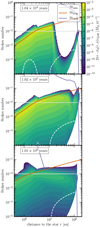Fig. B.3

As Fig. 5, but for an example run with accretion heating (the most appropriate simulation, see the last row in Table 1).

References

Andrews, S. M., Wilner, D., Hughes, A., Qi, C., & Dullemond, C. 2010, ApJ, 723, 1241 [NASA ADS] [CrossRef] [Google Scholar]
Armitage, P. J. 2010, Astrophysics of Planet Formation (Cambridge: Cambridge University Press) [Google Scholar]
Asplund, M., Grevesse, N., Sauval, A. J., & Scott, P. 2009, ARA&A, 47, 481 [NASA ADS] [CrossRef] [Google Scholar]
Baehr, H., Klahr, H., & Kratter, K. M. 2017, ApJ, 848, 40 [NASA ADS] [CrossRef] [Google Scholar]
Bai, X.-N., & Stone, J. M. 2014, ApJ, 796, 31 [Google Scholar]
Barge, P., & Sommeria, J. 1995, A&A, 295, L1 [NASA ADS] [Google Scholar]
Batygin, K., & Brown, M. E. 2010, ApJ, 716, 1323 [NASA ADS] [CrossRef] [Google Scholar]
Batygin, K., & Brown, M. E. 2016, AJ, 151, 22 [NASA ADS] [CrossRef] [Google Scholar]
Batygin, K., & Laughlin, G. 2015, Proc. Natl. Acad. Sci., 112, 4214 [Google Scholar]
Béthune, W., Lesur, G., & Ferreira, J. 2016, A&A, 589, A87 [NASA ADS] [CrossRef] [EDP Sciences] [Google Scholar]
Birnstiel, T., Dullemond, C. P., & Brauer, F. 2010, A&A, 513, A79 [NASA ADS] [CrossRef] [EDP Sciences] [Google Scholar]
Birnstiel, T., Klahr, H., & Ercolano, B. 2012, A&A, 539, A148 [NASA ADS] [CrossRef] [EDP Sciences] [Google Scholar]
Birnstiel, T., Dullemond, C. P., Zhu, Z., et al. 2018, ApJ, 869, L45 [NASA ADS] [CrossRef] [Google Scholar]
Blum, J., & Münch, M. 1993, Icarus, 106, 151 [NASA ADS] [CrossRef] [Google Scholar]
Blum, J., & Wurm, G. 2008, ARA&A, 46, 21 [NASA ADS] [CrossRef] [EDP Sciences] [Google Scholar]
Bordukat, S. 2019, Bachelor’s thesis, Ruperto-Carola University Heidelberg, Heidelberg [Google Scholar]
Bottke Jr, W. F., Nolan, M. C., Greenberg, R., & Kolvoord, R. A. 1994, Icarus, 107, 255 [NASA ADS] [CrossRef] [Google Scholar]
Bottke Jr, W. F., Durda, D. D., Nesvornỳ, D., et al. 2005a, Icarus, 175, 111 [NASA ADS] [CrossRef] [Google Scholar]
Bottke Jr, W. F., Durda, D. D., Nesvornỳ, D., et al. 2005b, Icarus, 179, 63 [NASA ADS] [CrossRef] [Google Scholar]
Brasser, R., Duncan, M., & Levison, H. 2006, Icarus, 184, 59 [NASA ADS] [CrossRef] [Google Scholar]
Brasser, R., Duncan, M., & Levison, H. 2007, Icarus, 191, 413 [NASA ADS] [CrossRef] [Google Scholar]
Brasser, R., Duncan, M., Levison, H., Schwamb, M., & Brown, M. 2012, Icarus, 217, 1 [NASA ADS] [CrossRef] [Google Scholar]
Brown, M. E., Trujillo, C., & Rabinowitz, D. 2004, ApJ, 617, 645 [NASA ADS] [CrossRef] [Google Scholar]
Campins, H., Davis, D., Weidenschilling, S., et al. 1996, ASP Conf. Ser. 107, 85 [NASA ADS] [Google Scholar]
Chapman, S. 1916, Phil. Trans. R. Soc. London. Ser. A, 216, 279 [CrossRef] [Google Scholar]
Chatterjee, S., & Tan, J. C. 2013, ApJ, 780, 53 [Google Scholar]
Cheng, N.-S. 2009, Powder Technol., 189, 395 [CrossRef] [Google Scholar]
Chiang, E., & Goldreich, P. 1997, ApJ, 490, 368 [NASA ADS] [CrossRef] [Google Scholar]
Chiang, E., & Laughlin, G. 2013, MNRAS, 431, 3444 [Google Scholar]
Cuzzi, J. N., Dobrovolskis, A. R., & Champney, J. M. 1993, Icarus, 106, 102 [NASA ADS] [CrossRef] [Google Scholar]
Cuzzi, J. N., Hogan, R. C., Paque, J. M., & Dobrovolskis, A. R. 2001, ApJ, 546, 496 [NASA ADS] [CrossRef] [Google Scholar]
Desch, S. J., Estrada, P. R., Kalyaan, A., & Cuzzi, J. N. 2017, ApJ, 840, 86 [NASA ADS] [CrossRef] [Google Scholar]
Dones, L., Weissman, P. R., Levison, H. F., & Duncan, M. J. 2004, ASP Conf. Ser., 323, 371 [NASA ADS] [Google Scholar]
Drążkowska, J., & Alibert, Y. 2017, A&A, 608, A92 [NASA ADS] [CrossRef] [EDP Sciences] [Google Scholar]
Drążkowska, J., Alibert, Y., & Moore, B. 2016, A&A, 594, A105 [NASA ADS] [CrossRef] [EDP Sciences] [Google Scholar]
Dubrulle, B., Morfill, G., & Sterzik, M. 1995, Icarus, 114, 237 [NASA ADS] [CrossRef] [Google Scholar]
Epstein, P. S. 1924, Phys. Rev., 23, 710 [NASA ADS] [CrossRef] [Google Scholar]
Eriksson, L. E., Johansen, A., & Liu, B. 2020, A&A, 635, A110 [CrossRef] [EDP Sciences] [Google Scholar]
Fernandez, J., & Ip, W.-H. 1984, Icarus, 58, 109 [NASA ADS] [CrossRef] [Google Scholar]
Fick, A. 1855, Ann. Phys., 170, 59 [NASA ADS] [CrossRef] [Google Scholar]
Fuentes, C. I., & Holman, M. J. 2008, AJ, 136, 83 [NASA ADS] [CrossRef] [Google Scholar]
Gerbig, K., Lenz, C. T., & Klahr, H. 2019, A&A, 629, A116 [CrossRef] [EDP Sciences] [Google Scholar]
Gerbig, K., Murray-Clay, R. A., Klahr, H., & Baehr, H. 2020, ApJ, 895, A91 [CrossRef] [Google Scholar]
Goldreich, P., & Lynden-Bell, D. 1965, MNRAS, 130, 97 [NASA ADS] [CrossRef] [Google Scholar]
Gomes, R., Levison, H. F., Tsiganis, K., & Morbidelli, A. 2005, Nature, 435, 466 [NASA ADS] [CrossRef] [PubMed] [Google Scholar]
Gough, D. 1981, Physics of Solar Variations (Berlin: Springer), 21 [Google Scholar]
Gradie, J. C., Chapman, C. R., & Tedesco, E. F. 1989, in Asteroids II, eds. R. P. Binzel, T. Gehrels, & M. S. Matthews (Tucson, AZ: University of Arizona Press), 316 [Google Scholar]
Güdel, M., Guinan, E. F., & Skinner, S. L. 1997, ApJ, 483, 947 [NASA ADS] [CrossRef] [Google Scholar]
Gundlach, B., & Blum, J. 2014, ApJ, 798, 34 [NASA ADS] [CrossRef] [Google Scholar]
Hansen, B. M. 2009, ApJ, 703, 1131 [NASA ADS] [CrossRef] [Google Scholar]
Hansen, B. M., & Murray, N. 2012, ApJ, 751, 158 [Google Scholar]
Hayashi, C. 1981, Prog. Theor. Phys. Suppl., 70, 35 [NASA ADS] [CrossRef] [MathSciNet] [Google Scholar]
Helled, R., & Schubert, G. 2008, Icarus, 198, 156 [NASA ADS] [CrossRef] [Google Scholar]
Hubeny, I. 1990, ApJ, 351, 632 [NASA ADS] [CrossRef] [Google Scholar]
Ida, S., & Lin, D. 2008, ApJ, 673, 487 [NASA ADS] [CrossRef] [Google Scholar]
Jewitt, D., Luu, J., & Trujillo, C. 1998, AJ, 115, 2125 [NASA ADS] [CrossRef] [Google Scholar]
Johansen, A., Klahr, H., & Henning, T. 2006, ApJ, 636, 1121 [NASA ADS] [CrossRef] [Google Scholar]
Johansen, A., Oishi, J. S., Mac Low, M.-M., et al. 2007, Nature, 448, 1022 [Google Scholar]
Johansen, A., Mac Low, M.-M., Lacerda, P., & Bizzarro, M. 2015, Sci. Adv., 1, e1500109 [NASA ADS] [CrossRef] [Google Scholar]
Kaib, N. A., & Quinn, T. 2008, Icarus, 197, 221 [NASA ADS] [CrossRef] [Google Scholar]
Klahr, H., & Bodenheimer, P. 2006, ApJ, 639, 432 [NASA ADS] [CrossRef] [Google Scholar]
Klahr, H., & Schreiber, A. 2015, Proc. IAU, 10, 1 [CrossRef] [Google Scholar]
Kokubo, E., Kominami, J., & Ida, S. 2006, ApJ, 642, 1131 [NASA ADS] [CrossRef] [Google Scholar]
Kresak, L. 1977, Bull. Astr. Inst. Czechosl., 28, 65 [Google Scholar]
Lambrechts, M., & Johansen, A. 2012, A&A, 544, A32 [Google Scholar]
Lenz, C. T., Klahr, H., & Birnstiel, T. 2019, ApJ, 874, 36 [CrossRef] [Google Scholar]
Levison, H. F., Thommes, E., & Duncan, M. J. 2010, AJ, 139, 1297 [NASA ADS] [CrossRef] [Google Scholar]
Levison, H. F., Morbidelli, A., Tsiganis, K., Nesvornỳ, D., & Gomes, R. 2011, AJ, 142, 152 [NASA ADS] [CrossRef] [Google Scholar]
Levison, H. F., Kretke, K. A., Walsh, K. J., & Bottke, W. F. 2015, Proc. Natl. Acad. Sci., 112, 14180 [NASA ADS] [CrossRef] [Google Scholar]
Lynden-Bell, D., & Pringle, J. 1974, MNRAS, 168, 603 [Google Scholar]
Malhotra, R. 1995, AJ, 110, 420 [NASA ADS] [CrossRef] [Google Scholar]
Massey, H., & Mohr, C. 1933, Proc. R. Soc. London, Ser. A, 141, 434 [CrossRef] [Google Scholar]
Minton, D. A., & Malhotra, R. 2010, Icarus, 207, 744 [NASA ADS] [CrossRef] [Google Scholar]
Morbidelli, A., Levison, H. F., Tsiganis, K., & Gomes, R. 2005, Nature, 435, 462 [NASA ADS] [CrossRef] [PubMed] [Google Scholar]
Morbidelli, A., Tsiganis, K., Crida, A., Levison, H. F., & Gomes, R. 2007, AJ, 134, 1790 [NASA ADS] [CrossRef] [Google Scholar]
Morbidelli, A., Crida, A., Masset, F., & Nelson, R. P. 2008, A&A, 478, 929 [NASA ADS] [CrossRef] [EDP Sciences] [Google Scholar]
Morbidelli, A., Bottke, W. F., Nesvornỳ, D., & Levison, H. F. 2009, Icarus, 204, 558 [NASA ADS] [CrossRef] [Google Scholar]
Morbidelli, A., Walsh, K. J., O’Brien, D. P., Minton, D. A., & Bottke, W. F. 2015, Asteroids IV (Tucson, AZ: University of Arizona Press), 493 [Google Scholar]
Morbidelli, A., Bitsch, B., Crida, A., et al. 2016, Icarus, 267, 368 [NASA ADS] [CrossRef] [Google Scholar]
Morfill, G., & Völk, H. 1984, ApJ, 287, 371 [NASA ADS] [CrossRef] [Google Scholar]
Musiolik, G., & Wurm, G. 2019, ApJ, 873, 58 [NASA ADS] [CrossRef] [Google Scholar]
Nakagawa, Y., Sekiya, M., & Hayashi, C. 1986, Icarus, 67, 375 [NASA ADS] [CrossRef] [Google Scholar]
Nakamoto, T., & Nakagawa, Y. 1994, ApJ, 421, 640 [NASA ADS] [CrossRef] [Google Scholar]
Nesvornỳ, D., & Morbidelli, A. 2012, AJ, 144, 117 [NASA ADS] [CrossRef] [Google Scholar]
Nesvornỳ, D., & Vokrouhlickỳ, D. 2016, ApJ, 825, 94 [NASA ADS] [CrossRef] [Google Scholar]
Nesvornỳ, D., Vokrouhlickỳ, D., Bottke, W. F., Noll, K., & Levison, H. F. 2011, AJ, 141, 159 [NASA ADS] [CrossRef] [Google Scholar]
Nesvornỳ, D., Vokrouhlickỳ, D., & Morbidelli, A. 2013, ApJ, 768, 45 [NASA ADS] [CrossRef] [Google Scholar]
Newton, I. 1729, The mathematical principles of natural philosophy. By Sir Isaac Newton. Translated into English by Andrew Motte. To which are added, The laws of the moon’s motion, according to gravity. By John Machin Astron. Prof. Gresh. and Secr. R. Soc. In two volumes (Benjamin Motte, at the Middle-Temple-Gate, in Fleetstreet) [Google Scholar]
O’Brien, D. P., & Greenberg, R. 2005, Icarus, 178, 179 [NASA ADS] [CrossRef] [Google Scholar]
Ormel, C. W. 2017, in Formation, Evolution, and Dynamics of Young Solar Systems (Berlin: Springer), 197 [Google Scholar]
Ormel, C., & Cuzzi, J. 2007, A&A, 466, 413 [NASA ADS] [CrossRef] [EDP Sciences] [Google Scholar]
Ormel, C., & Klahr, H. 2010, A&A, 520, A43 [NASA ADS] [CrossRef] [EDP Sciences] [Google Scholar]
Ostriker, J. P. 1963, ApJ, 138, 281 [CrossRef] [Google Scholar]
Owen, J. E., Clarke, C. J., & Ercolano, B. 2012, MNRAS, 422, 1880 [NASA ADS] [CrossRef] [Google Scholar]
Pan, M., & Sari, R. 2005, Icarus, 173, 342 [NASA ADS] [CrossRef] [Google Scholar]
Pfeil, T., & Klahr, H. 2019, ApJ, 871, 150 [NASA ADS] [CrossRef] [Google Scholar]
Picogna, G., Ercolano, B., Owen, J. E., & Weber, M. L. 2019, MNRAS, 487, 691 [NASA ADS] [CrossRef] [Google Scholar]
Pinilla, P., Birnstiel, T., Ricci, L., et al. 2012, A&A, 538, A114 [NASA ADS] [CrossRef] [EDP Sciences] [Google Scholar]
Pringle, J. E. 1981, ARA&A, 19, 137 [NASA ADS] [CrossRef] [Google Scholar]
Rayleigh, L. 1892, London, Edinburgh, Dublin Philos. Mag. J. Sci. 34, 59 [CrossRef] [Google Scholar]
Raymond, S. N., & Izidoro, A. 2017, Sci. Adv., 3, e1701138 [NASA ADS] [CrossRef] [Google Scholar]
Reeks, M. 1983, J. Aerosol Sci., 14, 729 [CrossRef] [Google Scholar]
Saumon, D., & Guillot, T. 2004, ApJ, 609, 1170 [NASA ADS] [CrossRef] [Google Scholar]
Schoonenberg,D., Ormel, C. W., & Krijt, S. 2018, A&A, 620, A134 [NASA ADS] [CrossRef] [EDP Sciences] [Google Scholar]
Schreiber, A. 2018, PhD thesis, Ruperto-Carola University Heidelberg, Heidelberg [Google Scholar]
Shakura, N. I., & Sunyaev, R. A. 1973, A&A, 24, 337 [NASA ADS] [Google Scholar]
Singer, K. N., McKinnon, W. B., Gladman, B., et al. 2019, Science, 363, 955 [NASA ADS] [CrossRef] [Google Scholar]
Stammler, S. M., Drążkowskaa, J., Birnstiel, T., et al. 2019, ApJ, 884, L5 [NASA ADS] [CrossRef] [Google Scholar]
Steffl, A., Cunningham, N., Shinn, A., Durda, D., & Stern, S. 2013, Icarus, 223, 48 [CrossRef] [Google Scholar]
Steinpilz, T., Joeris, K., Jungmann, F., et al. 2019, Nat. Phys., 1, 225 [Google Scholar]
Stokes, G. G. 1851, On the Effect of the Internal Friction of Fluids on the Motion of Pendulums, (Cambridge: Pitt Press Cambridge), 9 [Google Scholar]
Thommes, E. W., Duncan, M. J., & Levison, H. F. 1999, Nature, 402, 635 [NASA ADS] [CrossRef] [PubMed] [Google Scholar]
Thommes, E. W., & Duncan, M. J. 2006, Planet Formation, eds. H. Klahr, & W. Brandner (Cambridge: Cambridge University Press), 129 [CrossRef] [Google Scholar]
Toomre, A. 1964, ApJ, 139, 1217 [Google Scholar]
Trujillo, C. A., & Brown, M. E. 2001, ApJ, 554, L95 [NASA ADS] [CrossRef] [MathSciNet] [Google Scholar]
Tsiganis, K., Gomes, R., Morbidelli, A., & Levison, H. 2005, Nature, 435, 459 [NASA ADS] [CrossRef] [PubMed] [Google Scholar]
Tyrrell, H. J. V. 1964, J. Chem. Edu., 41, 397 [CrossRef] [Google Scholar]
Vagnozzi, S. 2019, Atoms, 7, 41 [NASA ADS] [CrossRef] [Google Scholar]
Vidotto, A. A., Gregory, S. G., Jardine, M., et al. 2014, MNRAS, 441, 2361 [NASA ADS] [CrossRef] [Google Scholar]
Volk, K., & Gladman, B. 2015, ApJ, 806, L26 [NASA ADS] [CrossRef] [Google Scholar]
von Smoluchowski, M. 1916, Z. Phys., 17, 557 [Google Scholar]
Wahl, S. M., Hubbard, W. B., Militzer, B., et al. 2017, Geophys. Res. Lett., 44, 4649 [NASA ADS] [CrossRef] [Google Scholar]
Walsh, K. J., Morbidelli, A., Raymond, S. N., O’Brien, D. P., & Mandell, A. M. 2011, Nature, 475, 206 [NASA ADS] [CrossRef] [PubMed] [Google Scholar]
Weidenschilling, S. J. 1977a, Astrophys. Space Sci., 51, 153 [NASA ADS] [CrossRef] [Google Scholar]
Weidenschilling, S. J. 1977b, MNRAS, 180, 57 [Google Scholar]
Whipple, F. L. 1972, in From Plasma to Planet (New York: Wiley Interscience Division,) 211 [Google Scholar]
Windmark, F., Birnstiel, T., Ormel, C. W., & Dullemond, C. P. 2012, A&A, 544, L16 [NASA ADS] [CrossRef] [EDP Sciences] [Google Scholar]
Wölfer, L., Picogna, G., Ercolano, B., & van Dishoeck, E. F. 2019, MNRAS, 490, 5596 [CrossRef] [Google Scholar]
Yang, C.-C., Johansen, A., & Carrera, D. 2017, A&A, 606, A80 [NASA ADS] [CrossRef] [EDP Sciences] [Google Scholar]
Youdin, A. N., & Goodman, J. 2005, ApJ, 620, 459 [NASA ADS] [CrossRef] [Google Scholar]
Youdin, A. N., & Lithwick, Y. 2007, Icarus, 192, 588 [NASA ADS] [CrossRef] [Google Scholar]
Zsom, A., Ormel, C., Güttler, C., Blum, J., & Dullemond, C. 2010, A&A, 513, A57 [NASA ADS] [CrossRef] [EDP Sciences] [Google Scholar]

¹

Following Weidenschilling (1977b), this condition can be obtained by setting either the stopping time in the Stokes drag law and the Epstein drag regime or the two drag forces equal and making use of Eq. (5).

²

The diffusive flux is sometimes written in a form where it is proportional to the gradient of concentration, which is meant in the sense of mass per volume, not mass over mass fraction. In our notation this is given by the density ρ.

All Tables

Table 1

Parameters used in this study.

In the text

Table 2

Parameters that can be excluded to reproduce the solar nebula based on Figs. 7, 8, 9, and 10.

In the text

Table 3

Parameter ranges that might work for reproducing the Solar System.

In the text

All Figures

	Fig. 1 Graphical representation summarizing Sect. 2 on mass constraints of initial planetesimal masses in different regions of the solar nebula. Masses given by the values on the ordinate apply for the entire marked regions. Boxes that extend to the border of the plot indicate unknown upper limits. The dotted vertical line separates the two touching regions.
In the text

	Fig. 2 As Fig. 1, but converted into column densities, assuming a power-law shape ∝ r^−2.25 (see Eq. (37) of Lenz et al. 2019 for a motivation). The blue (orange) line shows (three times) the minimum mass solar nebula profile for solids (Weidenschilling 1977a; Hayashi 1981).
In the text

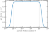	Fig. 3 Illustration of Eq. (31) for St_min = 0.01 and St_max = 10.
In the text

Fig. 4

Final mass in planetesimals within a given disk radius shown in the legend, normalized to the initial total disk dust mass, as a function of planetesimal formation efficiency. Defining ε = 5h_g ∕ℓ, where ℓ is theconversion length over which pebbles are transformed into planetesimals. The vertical dashed lines show the predicted maximum at the outer edge of the respective zone. This means that the dashed blue line shows the predicted maximum at 1 au and the purple line shows this at 50 au. This plot shows ε variations from the first fiducial run (gray values in Table 1) in the left panel and from the second fiducial run in the right panel (bold values in Table 1).

In the text

Fig. 5

Local particle flux in Earth masses per year resulting from pure radial drift per size bin (color) as a function of Stokes number and disk radius. Here, we show the first fiducial run in the left panels (gray values in Table 1) and the second fiducial run in the right panels (bold values in Table 1), both at three different snapshots. The orange (purple) line shows the fragmentation (drift) limit, and the gray line the threshold Stokes number that is required to participate in planetesimal formation (but see the smoothing function Eq. (31)). Particles in the region below the dashed white line have positive total radial velocities, i.e., they are moving outward. For the simulation shown in the left panels, outside of ~ 10 au the disk is limited by drift over most of the time of planetesimal formation. For the simulation shown in the right panels, the disk is mostly limited by fragmentation.

In the text

Fig. 6

Top panels: planetesimal (solid), gas (dashed), and total dust (dotted) vertically integrated density profiles at different times. Bottom panels: same quantities, but as a function of time, for three different disk locations. Both fiducial simulations are compared, where the first (gray values in Table 1) is shown in the right and the second (bold valuesin Table 1) in the left panels.

In the text

Fig. 7

Total planetesimal mass as a function of time for the first sample (gray values in Table 1). The fiducial values for this set of simulations are shown in the header of the plot. In each panel, the simulation with those parameters is shown as the dashed gray line, and the solid lines with colors show simulation results where only one parameter of the set was changed. The gray area shows values more massive than the solids of the MMSN (Weidenschilling 1977a; Hayashi 1981).

In the text

Fig. 8

Same as Fig. 7, but for the second sample (variations to the bold values in Table 1). The fiducial run produces just enough planetesimal mass in the disk to reach the MMSN mass in solids, even though the disk mass already is at the high end. From this point of view, either a higher initial dust-to-gas ratio, a higher planetesimal formation efficiency, or a higher fragmentation speed are required. Bottom left panel: no line is visible for α_t = 0.01 as no planetesimals are formed in that case.

In the text

Fig. 9

Final (at 10 Myr) planetesimal column density as a function of disk radius for the first sample (gray values in Table 1). The fiducialvalues for this set of simulations are shown in the header of the plot. In each panel, the simulation with those parameters is shown as dashed gray line, and the solid lines with colors show simulation results where only one parameter of the set was changed. The gray areas represent the constraints that we described in Sect. 2, where the mass in the given region was translated into a column density, assuming a planetesimal profile ∝ r^−2.25 (see Eq. (37) of Lenz et al. 2019). For the outermost region, we also overplotted a box ∝ r⁻⁸.

In the text

	Fig. 10 Same as Fig. 9, but for the second sample (variations to the bold values in Table 1). If ε is high enough, photoevaporation does not change the result significantly. It seems to have an effect for low ε, however; see the yellow line in the bottom middle panel of Fig. 8. Top left panel: we also plot the most appropriate case as a dotted line (last row in Table 1).
In the text

Fig. B.1

Pebble flux in units of Earth masses per year for different times as a function of disk radius (upper panel) and as a function oftime for different disk locations (lower panel). Here, we show data from the accretion heating simulation (the most appropriate case, see the last row in Table 1). Solid lines show the pebble flux using the smoothing function Eq. (31), dashed lines show the total flux, i.e., taking all solid material into account, except for planetesimals. For the upper panels, sub-critical fluxes are marked by the gray zone. They are shown in the respective colors in thelower panels.

In the text

	Fig. B.2 Same as Fig. 6, but for the accretion heating simulation (the most appropriate case, see the last row in Table 1).
In the text

	Fig. B.3 As Fig. 5, but for an example run with accretion heating (the most appropriate simulation, see the last row in Table 1).
In the text

Current usage metrics show cumulative count of Article Views (full-text article views including HTML views, PDF and ePub downloads, according to the available data) and Abstracts Views on Vision4Press platform.

Data correspond to usage on the plateform after 2015. The current usage metrics is available 48-96 hours after online publication and is updated daily on week days.

Initial download of the metrics may take a while.

[1] Andrews, S. M., Wilner, D., Hughes, A., Qi, C., & Dullemond, C. 2010, ApJ, 723, 1241 [NASA ADS] [CrossRef] [Google Scholar]

[2] Armitage, P. J. 2010, Astrophysics of Planet Formation (Cambridge: Cambridge University Press) [Google Scholar]

[3] Asplund, M., Grevesse, N., Sauval, A. J., & Scott, P. 2009, ARA&A, 47, 481 [NASA ADS] [CrossRef] [Google Scholar]

[4] Baehr, H., Klahr, H., & Kratter, K. M. 2017, ApJ, 848, 40 [NASA ADS] [CrossRef] [Google Scholar]

[5] Bai, X.-N., & Stone, J. M. 2014, ApJ, 796, 31 [Google Scholar]

[6] Barge, P., & Sommeria, J. 1995, A&A, 295, L1 [NASA ADS] [Google Scholar]

[7] Batygin, K., & Brown, M. E. 2010, ApJ, 716, 1323 [NASA ADS] [CrossRef] [Google Scholar]

[8] Batygin, K., & Brown, M. E. 2016, AJ, 151, 22 [NASA ADS] [CrossRef] [Google Scholar]

[9] Batygin, K., & Laughlin, G. 2015, Proc. Natl. Acad. Sci., 112, 4214 [Google Scholar]

[10] Béthune, W., Lesur, G., & Ferreira, J. 2016, A&A, 589, A87 [NASA ADS] [CrossRef] [EDP Sciences] [Google Scholar]

[11] Birnstiel, T., Dullemond, C. P., & Brauer, F. 2010, A&A, 513, A79 [NASA ADS] [CrossRef] [EDP Sciences] [Google Scholar]

[12] Birnstiel, T., Klahr, H., & Ercolano, B. 2012, A&A, 539, A148 [NASA ADS] [CrossRef] [EDP Sciences] [Google Scholar]

[13] Birnstiel, T., Dullemond, C. P., Zhu, Z., et al. 2018, ApJ, 869, L45 [NASA ADS] [CrossRef] [Google Scholar]

[14] Blum, J., & Münch, M. 1993, Icarus, 106, 151 [NASA ADS] [CrossRef] [Google Scholar]

[15] Blum, J., & Wurm, G. 2008, ARA&A, 46, 21 [NASA ADS] [CrossRef] [EDP Sciences] [Google Scholar]

[16] Bordukat, S. 2019, Bachelor’s thesis, Ruperto-Carola University Heidelberg, Heidelberg [Google Scholar]

[17] Bottke Jr, W. F., Nolan, M. C., Greenberg, R., & Kolvoord, R. A. 1994, Icarus, 107, 255 [NASA ADS] [CrossRef] [Google Scholar]

[18] Bottke Jr, W. F., Durda, D. D., Nesvornỳ, D., et al. 2005a, Icarus, 175, 111 [NASA ADS] [CrossRef] [Google Scholar]

[19] Bottke Jr, W. F., Durda, D. D., Nesvornỳ, D., et al. 2005b, Icarus, 179, 63 [NASA ADS] [CrossRef] [Google Scholar]

[20] Brasser, R., Duncan, M., & Levison, H. 2006, Icarus, 184, 59 [NASA ADS] [CrossRef] [Google Scholar]

[21] Brasser, R., Duncan, M., & Levison, H. 2007, Icarus, 191, 413 [NASA ADS] [CrossRef] [Google Scholar]

[22] Brasser, R., Duncan, M., Levison, H., Schwamb, M., & Brown, M. 2012, Icarus, 217, 1 [NASA ADS] [CrossRef] [Google Scholar]

[23] Brown, M. E., Trujillo, C., & Rabinowitz, D. 2004, ApJ, 617, 645 [NASA ADS] [CrossRef] [Google Scholar]

[24] Campins, H., Davis, D., Weidenschilling, S., et al. 1996, ASP Conf. Ser. 107, 85 [NASA ADS] [Google Scholar]

[25] Chapman, S. 1916, Phil. Trans. R. Soc. London. Ser. A, 216, 279 [CrossRef] [Google Scholar]

[26] Chatterjee, S., & Tan, J. C. 2013, ApJ, 780, 53 [Google Scholar]

[27] Cheng, N.-S. 2009, Powder Technol., 189, 395 [CrossRef] [Google Scholar]

[28] Chiang, E., & Goldreich, P. 1997, ApJ, 490, 368 [NASA ADS] [CrossRef] [Google Scholar]

[29] Chiang, E., & Laughlin, G. 2013, MNRAS, 431, 3444 [Google Scholar]

[30] Cuzzi, J. N., Dobrovolskis, A. R., & Champney, J. M. 1993, Icarus, 106, 102 [NASA ADS] [CrossRef] [Google Scholar]

[31] Cuzzi, J. N., Hogan, R. C., Paque, J. M., & Dobrovolskis, A. R. 2001, ApJ, 546, 496 [NASA ADS] [CrossRef] [Google Scholar]

[32] Desch, S. J., Estrada, P. R., Kalyaan, A., & Cuzzi, J. N. 2017, ApJ, 840, 86 [NASA ADS] [CrossRef] [Google Scholar]

[33] Dones, L., Weissman, P. R., Levison, H. F., & Duncan, M. J. 2004, ASP Conf. Ser., 323, 371 [NASA ADS] [Google Scholar]

[34] Drążkowska, J., & Alibert, Y. 2017, A&A, 608, A92 [NASA ADS] [CrossRef] [EDP Sciences] [Google Scholar]

[35] Drążkowska, J., Alibert, Y., & Moore, B. 2016, A&A, 594, A105 [NASA ADS] [CrossRef] [EDP Sciences] [Google Scholar]

[36] Dubrulle, B., Morfill, G., & Sterzik, M. 1995, Icarus, 114, 237 [NASA ADS] [CrossRef] [Google Scholar]

[37] Epstein, P. S. 1924, Phys. Rev., 23, 710 [NASA ADS] [CrossRef] [Google Scholar]

[38] Eriksson, L. E., Johansen, A., & Liu, B. 2020, A&A, 635, A110 [CrossRef] [EDP Sciences] [Google Scholar]

[39] Fernandez, J., & Ip, W.-H. 1984, Icarus, 58, 109 [NASA ADS] [CrossRef] [Google Scholar]

[40] Fick, A. 1855, Ann. Phys., 170, 59 [NASA ADS] [CrossRef] [Google Scholar]

[41] Fuentes, C. I., & Holman, M. J. 2008, AJ, 136, 83 [NASA ADS] [CrossRef] [Google Scholar]

[42] Gerbig, K., Lenz, C. T., & Klahr, H. 2019, A&A, 629, A116 [CrossRef] [EDP Sciences] [Google Scholar]

[43] Gerbig, K., Murray-Clay, R. A., Klahr, H., & Baehr, H. 2020, ApJ, 895, A91 [CrossRef] [Google Scholar]

[44] Goldreich, P., & Lynden-Bell, D. 1965, MNRAS, 130, 97 [NASA ADS] [CrossRef] [Google Scholar]

[45] Gomes, R., Levison, H. F., Tsiganis, K., & Morbidelli, A. 2005, Nature, 435, 466 [NASA ADS] [CrossRef] [PubMed] [Google Scholar]

[46] Gough, D. 1981, Physics of Solar Variations (Berlin: Springer), 21 [Google Scholar]

[47] Gradie, J. C., Chapman, C. R., & Tedesco, E. F. 1989, in Asteroids II, eds. R. P. Binzel, T. Gehrels, & M. S. Matthews (Tucson, AZ: University of Arizona Press), 316 [Google Scholar]

[48] Güdel, M., Guinan, E. F., & Skinner, S. L. 1997, ApJ, 483, 947 [NASA ADS] [CrossRef] [Google Scholar]

[49] Gundlach, B., & Blum, J. 2014, ApJ, 798, 34 [NASA ADS] [CrossRef] [Google Scholar]

[50] Hansen, B. M. 2009, ApJ, 703, 1131 [NASA ADS] [CrossRef] [Google Scholar]

[51] Hansen, B. M., & Murray, N. 2012, ApJ, 751, 158 [Google Scholar]

[52] Hayashi, C. 1981, Prog. Theor. Phys. Suppl., 70, 35 [NASA ADS] [CrossRef] [MathSciNet] [Google Scholar]

[53] Helled, R., & Schubert, G. 2008, Icarus, 198, 156 [NASA ADS] [CrossRef] [Google Scholar]

[54] Hubeny, I. 1990, ApJ, 351, 632 [NASA ADS] [CrossRef] [Google Scholar]

[55] Ida, S., & Lin, D. 2008, ApJ, 673, 487 [NASA ADS] [CrossRef] [Google Scholar]

[56] Jewitt, D., Luu, J., & Trujillo, C. 1998, AJ, 115, 2125 [NASA ADS] [CrossRef] [Google Scholar]

[57] Johansen, A., Klahr, H., & Henning, T. 2006, ApJ, 636, 1121 [NASA ADS] [CrossRef] [Google Scholar]

[58] Johansen, A., Oishi, J. S., Mac Low, M.-M., et al. 2007, Nature, 448, 1022 [Google Scholar]

[59] Johansen, A., Mac Low, M.-M., Lacerda, P., & Bizzarro, M. 2015, Sci. Adv., 1, e1500109 [NASA ADS] [CrossRef] [Google Scholar]

[60] Kaib, N. A., & Quinn, T. 2008, Icarus, 197, 221 [NASA ADS] [CrossRef] [Google Scholar]

[61] Klahr, H., & Bodenheimer, P. 2006, ApJ, 639, 432 [NASA ADS] [CrossRef] [Google Scholar]

[62] Klahr, H., & Schreiber, A. 2015, Proc. IAU, 10, 1 [CrossRef] [Google Scholar]

[63] Kokubo, E., Kominami, J., & Ida, S. 2006, ApJ, 642, 1131 [NASA ADS] [CrossRef] [Google Scholar]

[64] Kresak, L. 1977, Bull. Astr. Inst. Czechosl., 28, 65 [Google Scholar]

[65] Lambrechts, M., & Johansen, A. 2012, A&A, 544, A32 [Google Scholar]

[66] Lenz, C. T., Klahr, H., & Birnstiel, T. 2019, ApJ, 874, 36 [CrossRef] [Google Scholar]

[67] Levison, H. F., Thommes, E., & Duncan, M. J. 2010, AJ, 139, 1297 [NASA ADS] [CrossRef] [Google Scholar]

[68] Levison, H. F., Morbidelli, A., Tsiganis, K., Nesvornỳ, D., & Gomes, R. 2011, AJ, 142, 152 [NASA ADS] [CrossRef] [Google Scholar]

[69] Levison, H. F., Kretke, K. A., Walsh, K. J., & Bottke, W. F. 2015, Proc. Natl. Acad. Sci., 112, 14180 [NASA ADS] [CrossRef] [Google Scholar]

[70] Lynden-Bell, D., & Pringle, J. 1974, MNRAS, 168, 603 [Google Scholar]

[71] Malhotra, R. 1995, AJ, 110, 420 [NASA ADS] [CrossRef] [Google Scholar]

[72] Massey, H., & Mohr, C. 1933, Proc. R. Soc. London, Ser. A, 141, 434 [CrossRef] [Google Scholar]

[73] Minton, D. A., & Malhotra, R. 2010, Icarus, 207, 744 [NASA ADS] [CrossRef] [Google Scholar]

[74] Morbidelli, A., Levison, H. F., Tsiganis, K., & Gomes, R. 2005, Nature, 435, 462 [NASA ADS] [CrossRef] [PubMed] [Google Scholar]

[75] Morbidelli, A., Tsiganis, K., Crida, A., Levison, H. F., & Gomes, R. 2007, AJ, 134, 1790 [NASA ADS] [CrossRef] [Google Scholar]

[76] Morbidelli, A., Crida, A., Masset, F., & Nelson, R. P. 2008, A&A, 478, 929 [NASA ADS] [CrossRef] [EDP Sciences] [Google Scholar]

[77] Morbidelli, A., Bottke, W. F., Nesvornỳ, D., & Levison, H. F. 2009, Icarus, 204, 558 [NASA ADS] [CrossRef] [Google Scholar]

[78] Morbidelli, A., Walsh, K. J., O’Brien, D. P., Minton, D. A., & Bottke, W. F. 2015, Asteroids IV (Tucson, AZ: University of Arizona Press), 493 [Google Scholar]

[79] Morbidelli, A., Bitsch, B., Crida, A., et al. 2016, Icarus, 267, 368 [NASA ADS] [CrossRef] [Google Scholar]

[80] Morfill, G., & Völk, H. 1984, ApJ, 287, 371 [NASA ADS] [CrossRef] [Google Scholar]

[81] Musiolik, G., & Wurm, G. 2019, ApJ, 873, 58 [NASA ADS] [CrossRef] [Google Scholar]

[82] Nakagawa, Y., Sekiya, M., & Hayashi, C. 1986, Icarus, 67, 375 [NASA ADS] [CrossRef] [Google Scholar]

[83] Nakamoto, T., & Nakagawa, Y. 1994, ApJ, 421, 640 [NASA ADS] [CrossRef] [Google Scholar]

[84] Nesvornỳ, D., & Morbidelli, A. 2012, AJ, 144, 117 [NASA ADS] [CrossRef] [Google Scholar]

[85] Nesvornỳ, D., & Vokrouhlickỳ, D. 2016, ApJ, 825, 94 [NASA ADS] [CrossRef] [Google Scholar]

[86] Nesvornỳ, D., Vokrouhlickỳ, D., Bottke, W. F., Noll, K., & Levison, H. F. 2011, AJ, 141, 159 [NASA ADS] [CrossRef] [Google Scholar]

[87] Nesvornỳ, D., Vokrouhlickỳ, D., & Morbidelli, A. 2013, ApJ, 768, 45 [NASA ADS] [CrossRef] [Google Scholar]

[88] Newton, I. 1729, The mathematical principles of natural philosophy. By Sir Isaac Newton. Translated into English by Andrew Motte. To which are added, The laws of the moon’s motion, according to gravity. By John Machin Astron. Prof. Gresh. and Secr. R. Soc. In two volumes (Benjamin Motte, at the Middle-Temple-Gate, in Fleetstreet) [Google Scholar]

[89] O’Brien, D. P., & Greenberg, R. 2005, Icarus, 178, 179 [NASA ADS] [CrossRef] [Google Scholar]

[90] Ormel, C. W. 2017, in Formation, Evolution, and Dynamics of Young Solar Systems (Berlin: Springer), 197 [Google Scholar]

[91] Ormel, C., & Cuzzi, J. 2007, A&A, 466, 413 [NASA ADS] [CrossRef] [EDP Sciences] [Google Scholar]

[92] Ormel, C., & Klahr, H. 2010, A&A, 520, A43 [NASA ADS] [CrossRef] [EDP Sciences] [Google Scholar]

[93] Ostriker, J. P. 1963, ApJ, 138, 281 [CrossRef] [Google Scholar]

[94] Owen, J. E., Clarke, C. J., & Ercolano, B. 2012, MNRAS, 422, 1880 [NASA ADS] [CrossRef] [Google Scholar]

[95] Pan, M., & Sari, R. 2005, Icarus, 173, 342 [NASA ADS] [CrossRef] [Google Scholar]

[96] Pfeil, T., & Klahr, H. 2019, ApJ, 871, 150 [NASA ADS] [CrossRef] [Google Scholar]

[97] Picogna, G., Ercolano, B., Owen, J. E., & Weber, M. L. 2019, MNRAS, 487, 691 [NASA ADS] [CrossRef] [Google Scholar]

[98] Pinilla, P., Birnstiel, T., Ricci, L., et al. 2012, A&A, 538, A114 [NASA ADS] [CrossRef] [EDP Sciences] [Google Scholar]

[99] Pringle, J. E. 1981, ARA&A, 19, 137 [NASA ADS] [CrossRef] [Google Scholar]

[100] Rayleigh, L. 1892, London, Edinburgh, Dublin Philos. Mag. J. Sci. 34, 59 [CrossRef] [Google Scholar]

[101] Raymond, S. N., & Izidoro, A. 2017, Sci. Adv., 3, e1701138 [NASA ADS] [CrossRef] [Google Scholar]

[102] Reeks, M. 1983, J. Aerosol Sci., 14, 729 [CrossRef] [Google Scholar]

[103] Saumon, D., & Guillot, T. 2004, ApJ, 609, 1170 [NASA ADS] [CrossRef] [Google Scholar]

[104] Schoonenberg,D., Ormel, C. W., & Krijt, S. 2018, A&A, 620, A134 [NASA ADS] [CrossRef] [EDP Sciences] [Google Scholar]

[105] Schreiber, A. 2018, PhD thesis, Ruperto-Carola University Heidelberg, Heidelberg [Google Scholar]

[106] Shakura, N. I., & Sunyaev, R. A. 1973, A&A, 24, 337 [NASA ADS] [Google Scholar]

[107] Singer, K. N., McKinnon, W. B., Gladman, B., et al. 2019, Science, 363, 955 [NASA ADS] [CrossRef] [Google Scholar]

[108] Stammler, S. M., Drążkowskaa, J., Birnstiel, T., et al. 2019, ApJ, 884, L5 [NASA ADS] [CrossRef] [Google Scholar]

[109] Steffl, A., Cunningham, N., Shinn, A., Durda, D., & Stern, S. 2013, Icarus, 223, 48 [CrossRef] [Google Scholar]

[110] Steinpilz, T., Joeris, K., Jungmann, F., et al. 2019, Nat. Phys., 1, 225 [Google Scholar]

[111] Stokes, G. G. 1851, On the Effect of the Internal Friction of Fluids on the Motion of Pendulums, (Cambridge: Pitt Press Cambridge), 9 [Google Scholar]

[112] Thommes, E. W., Duncan, M. J., & Levison, H. F. 1999, Nature, 402, 635 [NASA ADS] [CrossRef] [PubMed] [Google Scholar]

[113] Thommes, E. W., & Duncan, M. J. 2006, Planet Formation, eds. H. Klahr, & W. Brandner (Cambridge: Cambridge University Press), 129 [CrossRef] [Google Scholar]

[114] Toomre, A. 1964, ApJ, 139, 1217 [Google Scholar]

[115] Trujillo, C. A., & Brown, M. E. 2001, ApJ, 554, L95 [NASA ADS] [CrossRef] [MathSciNet] [Google Scholar]

[116] Tsiganis, K., Gomes, R., Morbidelli, A., & Levison, H. 2005, Nature, 435, 459 [NASA ADS] [CrossRef] [PubMed] [Google Scholar]

[117] Tyrrell, H. J. V. 1964, J. Chem. Edu., 41, 397 [CrossRef] [Google Scholar]

[118] Vagnozzi, S. 2019, Atoms, 7, 41 [NASA ADS] [CrossRef] [Google Scholar]

[119] Vidotto, A. A., Gregory, S. G., Jardine, M., et al. 2014, MNRAS, 441, 2361 [NASA ADS] [CrossRef] [Google Scholar]

[120] Volk, K., & Gladman, B. 2015, ApJ, 806, L26 [NASA ADS] [CrossRef] [Google Scholar]

[121] von Smoluchowski, M. 1916, Z. Phys., 17, 557 [Google Scholar]

[122] Wahl, S. M., Hubbard, W. B., Militzer, B., et al. 2017, Geophys. Res. Lett., 44, 4649 [NASA ADS] [CrossRef] [Google Scholar]

[123] Walsh, K. J., Morbidelli, A., Raymond, S. N., O’Brien, D. P., & Mandell, A. M. 2011, Nature, 475, 206 [NASA ADS] [CrossRef] [PubMed] [Google Scholar]

[124] Weidenschilling, S. J. 1977a, Astrophys. Space Sci., 51, 153 [NASA ADS] [CrossRef] [Google Scholar]

[125] Weidenschilling, S. J. 1977b, MNRAS, 180, 57 [Google Scholar]

[126] Whipple, F. L. 1972, in From Plasma to Planet (New York: Wiley Interscience Division,) 211 [Google Scholar]

[127] Windmark, F., Birnstiel, T., Ormel, C. W., & Dullemond, C. P. 2012, A&A, 544, L16 [NASA ADS] [CrossRef] [EDP Sciences] [Google Scholar]

[128] Wölfer, L., Picogna, G., Ercolano, B., & van Dishoeck, E. F. 2019, MNRAS, 490, 5596 [CrossRef] [Google Scholar]

[129] Yang, C.-C., Johansen, A., & Carrera, D. 2017, A&A, 606, A80 [NASA ADS] [CrossRef] [EDP Sciences] [Google Scholar]

[130] Youdin, A. N., & Goodman, J. 2005, ApJ, 620, 459 [NASA ADS] [CrossRef] [Google Scholar]

[131] Youdin, A. N., & Lithwick, Y. 2007, Icarus, 192, 588 [NASA ADS] [CrossRef] [Google Scholar]

[132] Zsom, A., Ormel, C., Güttler, C., Blum, J., & Dullemond, C. 2010, A&A, 513, A57 [NASA ADS] [CrossRef] [EDP Sciences] [Google Scholar]