| Issue |
A&A
Volume 637, May 2020
|
|
|---|---|---|
| Article Number | A78 | |
| Number of page(s) | 14 | |
| Section | Planets and planetary systems | |
| DOI | https://doi.org/10.1051/0004-6361/201937317 | |
| Published online | 20 May 2020 | |
Tidal and general relativistic effects in rocky planet formation at the substellar mass limit using N-body simulations
1
Facultad de Ciencias Astronómicas y Geofísicas, Universidad Nacional de La Plata,
Paseo del Bosque s/n (1900),
La Plata,
Argentina
e-mail: This email address is being protected from spambots. You need JavaScript enabled to view it.
2
Instituto de Astrofísica de La Plata, CCT La Plata-CONICET-UNLP,
Paseo del Bosque s/n (1900),
La Plata,
Argentina
3
Centro Universitario Regional del Este, Universidad de la República,
AP 264,
Rocha
27000,
Uruguay
Received:
13
December
2019
Accepted:
10
March
2020
Abstract
Context. Recent observational results show that very low mass stars and brown dwarfs are able to host close-in rocky planets. Low-mass stars are the most abundant stars in the Galaxy, and the formation efficiency of their planetary systems is relevant in the computation of a global probability of finding Earth-like planets inside habitable zones. Tidal forces and relativistic effects are relevant in the latest dynamical evolution of planets around low-mass stars, and their effect on the planetary formation efficiency still needs to be addressed.
Aims. Our goal is to evaluate the impact of tidal forces and relativistic effects on the formation of rocky planets around a star close to the substellar mass limit in terms of the resulting planetary architectures and its distribution according to the corresponding evolving habitable zone.
Methods. We performed a set of N-body simulations spanning the first 100 Myr of the evolution of two systems composed of 224 embryos with a total mass 0.25 M⊕ and 74 embryos with a total mass 3 M⊕ around a central object of 0.08 M⊙. For these two scenarios we compared the planetary architectures that result from simulations that are purely gravitational with those from simulations that include the early contraction and spin-up of the central object, the distortions and dissipation tidal terms, and general relativistic effects.
Results. We found that including these effects allows the formation and survival of a close-in (r < 0.07 au) population of rocky planets with masses in the range 0.001 < m∕M⊕ < 0.02 in all the simulations of the less massive scenario, and a close-in population with masses m ~ 0.35 M⊕ in just a few of the simulations of the more massive scenario. The surviving close-in bodies suffered more collisions during the integration time of the simulations. These collisions play an important role in their final masses. However, all of these bodies conserved their initial amount of water in mass throughout the integration time.
Conclusions. The incorporation of tidal and general relativistic effects allows the formation of an in situ close-in population located in the habitable zone of the system. This means that both effects are relevant during the formation of rocky planets and their early evolution around stars close to the substellar mass limit, in particular when low-mass planetary embryos are involved.
Key words: planets and satellites: formation / planets and satellites: terrestrial planets / stars: low-mass / planet-star interactions / methods: numerical
© ESO 2020
1 Introduction
During the past decades several observational and theoretical results have suggested that the formation of rocky planets is a common process around stars of different masses (e.g., Cumming et al. 2008; Mordasini et al. 2009; Howard 2013; Ronco et al. 2017). In particular, observations and modeling have proven the existence and formation of rocky planets around very low mass stars (VLMS) and brown dwarfs (BDs; e.g., Payne & Lodato 2007; Raymond et al. 2007; Gillon et al. 2017). These achievements are relevant because VLMS are the most abundant stars in the Galaxy and together with BDs are within the closest solar neighbors (e.g., Padoan & Nordlund 2004; Henry 2004; Bastian et al. 2010). This allows for surveys of rocky planets even in habitable zones, around numerous stellar samples, and through different observational techniques. This could be a crucial observational test of the processes driving the planet formation as suggested by theoretical modeling.
Although the detection of rocky planets around BDs is still challenging, some systems have been discovered (e.g., Kubas et al. 2012; Gillon et al. 2017; Grimm et al. 2018; Zechmeister et al. 2019). Using photometry from Spitzer, He et al. (2017) reported an occurrence rate of ~87% of planets with radius 0.75 < R∕R⊕ < 1.25 and orbital periods 1.7 < P∕days < 1000 around a sample of 44 BDs. From the M-type low-mass stars monitored by the Kepler mission, Mulders et al. (2015) found that planets around VLMS are located close to their host stars, having an occurrence rate of small planets (1 < R∕R⊕ < 3), which is three to four times higher than for Sun-like stars, while Hardegree-Ullman et al. (2019) estimated a mean number of 1.19 planets per mid-type M dwarf with radius 0.5 < R∕R⊕ < 2.5 and orbital period 0.5 < P∕days < 10. The current SPHERE (Spectro-Polarimetric High-contrast Exoplanet REsearch) together with ESPRESSO (Echelle SPectrograph for Rocky Exoplanet and Stable Spectroscopic Observations) are already detecting Earth-sized planets around G, K, and M dwarfs (Lovis et al. 2017; Hojjatpanah et al. 2019), and CARMENES (Calar Alto High-Resolution Search for M Dwarfs with Exo-earths with a Near-infrared Echelle Spectrograph) is searching for exoplanets around M dwarfs and already found two Earth-mass planets around an M7 BD (Zechmeister et al. 2019). The ongoing and upcoming transit searches such as TESS (Transiting Exoplanet Survey Satellite) and PLATO (PLAnetary Transits and Oscillations of stars) are expected to find most of the nearest transiting systems in the next years (Barclay et al. 2018; Ragazzoni et al. 2016), opening the new era of atmospheric characterization of terrestrial-sized planets.
Current observations suggest that there does not seem to be a discontinuity in the general properties of the circumstellar disks around VLMS and BDs (e.g., Luhman 2012). In particular, the dust growth to millimeter and centimeters sizes on the disk mid-plane of BDs is similar to the growth in VLMS disks, as has been inferred for a few BDs that have been observed with ALMA (Atacama Large Milimeter Array) and CARMA (Combined Array for Research in Milimeter-wave Astronomy; Ricci et al. 2012, 2013, 2014). This suggests that similar processes in the evolution of the disk might also take place at either side of the substellar mass limit.
Payne & Lodato (2007) investigated planet formation around low-mass objects using a standard core accretion model. They found that the formation of Earth-like planets is possible even around BDs, and that planets with masses up to 5 M⊕ can be formed. They reported that the mass-distribution of the resulting planets is strongly correlated with the disk masses. In particular, if the BD has a disk mass of about a few Jupiter masses, then only 10% of the BDs might host planets with masses exceeding 0.3 M⊕. Through dynamical simulations of terrestrial planet formation from planetary embryos, Raymond et al. (2007) found that the masses of planets located inside the habitable zone decrease while the mass of the host star decreases. The authors found small and dry planets around low-mass stars. Using N-body simulations with diverse water-mass fractions for objects beyond the snow line, Ciesla et al. (2015) found both dry and water-rich planets close to low-mass stars. By studying planet formation around different host stars, their simulations predict that a greater number of compact and low-mass planets are located around low-mass stars, while higher mass stars will be hosting fewer and more massive planets. Recently, Coleman et al. (2019) studied planet formation around low-mass stars similar to Trappist-1 and considered different accretion scenarios. They found water-rich rocky planets with periods 0.5 < P∕days < 1000. Furthermore, Miguel et al. (2020) studied planet formation around BDs and low-mass stars using a population synthesis code and found planets with a high ice-to-rock ratio.
It is still debated how the formation and evolution of rocky planetary systems around low-mass objects needs to be treated. Planets around these objects are thought to form close to them in a region where tides are very strong and lead to significant orbital changes (Papaloizou & Terquem 2010; Barnes et al. 2010; Heller et al. 2010). That BDs as well as VLMS collapse and spin up with time in their first 100 Myr allows the population of close-in tidally locked bodies around them to experience many different dynamical evolutions (Bolmont et al. 2011). Bolmont et al. (2013, 2015) showed the importance of incorporating tidal effects and general relativity as well as the effect of rotation-induced flattering in the dynamical and tidal evolution of multi-planetary systems, particularly those with close-in bodies.
In this work we incorporate these effects in a set of N-body simulations to study rocky planet formation from a sample of embryos around an object with a mass of 0.08 M⊙ close to the substellar mass limit in a period of 100 Myr in order to improve predictions for planetary system architectures. We evaluatehow relevant tidal and relativistic effects are during rocky planet formation around an object at the substellar mass limit. Our aim is to estimate dynamical properties of the resulting population of close-in bodies and the efficiency of forming planets that remain in the habitable zone of the system.
In Sect. 2 we briefly describe the early gravitational collapse and rotation rates of VLMS and BDs. In Sect. 3 we model the habitable zone around a star close to the substellar mass limit. In Sect. 4 we describe the protoplanetary disk model that is based on observations. In Sect. 5 we explain the numerical method we used to include tidal forces and general relativity effects in the N-body simulations. In Sect. 6 we describe the resulting planetary systems, and in Sect. 7 we finally summarize our conclusions and future works.
2 Collapse and rotation of young VLMS and BD
The BDs are stellar structures that are unable to reach the necessary core temperatures and densities to sustain stable hydrogen fusion. For solar metallicity, the substellar mass limit that separates BDs from VLMS is 0.072 M⊙ (Baraffe et al. 2015). During the first ~100 Myr of their evolution, BDs and VLMS share several properties such as circumstellar disks at different evolutionary stages (e.g., Luhman 2012), the formation of planets around them, their gravitational collapse, and the subsequent increase in their rotation rates with time. These last two properties are particularly relevant in our modeling.
In the case of VLMS, the collapse stops when they reach the main sequence at ages of ~ 100 Myr. Brown dwarfs continue to collapse slowly toward to a degenerate structure that is unable to sustain stable hydrogen fusion (e.g., Kumar 1963; Hayashi & Nakano 1963).
Available observations show that the mean rotational periods of BD are shorter than those of VLMS. This has been interpreted as indicating that the magnetic braking on the early spin-up in the substellar mass domain is inefficient (Mohanty et al. 2002; Scholz et al. 2015). The spin rate of the main object sets the position of the corotation radius rcorot, which is the mid-plane orbital distance at which the mean orbital velocity n of a planet is equal to the rotational velocity Ω⋆ of the central object. In the case of a VLMS and BD, rcorot shrinks while the object spins up. This behavior is essential for the treatment of close-in bodies because their orbital evolution depends on the initial eccentricity e and semimajor axis a with respect to the location of rcorot.
3 Modeling the habitable zone
The classical habitable zone (CHZ) is the circular region around a single star or a multiple star system in which a rocky planet can retain liquid water on its surface (Kasting et al. 1993). The CHZ definition assumes that the most important greenhouse gases for habitable planets orbiting main-sequence stars are CO2 and H2 O. This assumption extends the idea that the long-term (~1 Myr) carbonate-silicate cycle on Earth acts as a planetary thermostat that regulates the surface temperature (Watson et al. 1981; Walker et al. 1981; Kasting 1988) toward potentially habitable exoplanets.
To study potentially habitable exoplanets around a nonsolar-type star, it is necessary to take the relation between the albedo and the effective temperature of the central star into account. By extrapolating the cases studied by Kasting et al. (1993), the inner and outer limits of the isolated habitable zone (IHZ) for stars with effective temperatures in between 3700 < Teff∕K < 7200 can be calculated as in Selsis et al. (2007) by
 (1)
(1)
 (2)
(2)
where lin,⊙ = 0.97 au and lout,⊙ = 1.67 au are the inner and outer limits of a system with a Sun-like star as central object, considering runaway greenhouse and maximum greenhouse values, respectively (Kopparapu et al. 2013a,b), and ain = 2.7619 × 10⁻⁵ au K−1, bin = 3.8095 × 10⁻⁹ au K−2, aout = 1.3786 × 10⁻⁴ au K−1, and bout = 1.4286 × 10⁻⁹ au K−2 are empirically determined constants; L⊙ and L⋆ are the luminosity of the Sun and the considered star, and the temperature of the star is T⋆ = Teff−5700 K, where Teff can be expressed by
 (3)
(3)
with R⋆ the radius of the central object and σ the Stefan-Boltzmann constant. As in Barnes et al. (2013), who studied habitable planets around BDs, we extended the calculation of the IHZ to the substellar mass limit. In this work lin and lout therefore represent the inner and outer limits of the IHZ around a 0.08 M⊙ object. We used R⋆, L⋆, and Teff as a function of time as predicted by the models of Baraffe et al. (2015)1. In Fig. 1 we show the evolution of the IHZ of an object of 0.08 M⊙. While the object is evolving, L⋆, R⋆, and Teff decrease with time and the location of the IHZ becomes narrower and closer to the substellar object. When the central object is 1 Myr old, lin =0.214 au and lout = 0.369 au, while at 1 Gyr, lin = 0.017 au and lout = 0.029 au. It is worth noting that the IHZ is located more than ten times closer to the central object after this time.
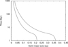 |
Fig. 1 Evolution of the habitable zone around a star of 0.08 M⊙ in a period of 1 Gyr. |
4 Protoplanetary disk
In this section, we describe the protoplanetary disk model that we adopted for the 0.08 M⊙ central object. We calculate the dust species that might survive inside our region of study to determine the material that is avialable for the formation of larger structures such as protoplanetary embryos. We distinguish two scenarios, motivated by the diversity of disk masses and the observed distribution of the exoplanet mass around low-mass objects. Finally, we compare our model with others that have been used by different authors.
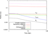 |
Fig. 2 Sublimation radii for different dust grain species and comparison with the corotation rcorot, the stellar radius R⋆, and the inner radii of our region of study rinit. |
4.1 Region of study
Our region of study is defined between an inner radius rinit = 0.015 au and an outer radius of rfinal = 1 au. The inner radius was selected by considering that tidal effects allow a planet located at this distance to survive without colliding with the central object for certain values of its eccentricity (Bolmont et al. 2011). The outer radius was defined in a way that the habitable zone and an outer region of water-rich embryos are contained in our region of study.
We evaluated the consistency of the selection of rinit with the sublimation radius for different dust species by analyzing those species that could survive inside our region of study. We computed sublimation radii for a variety of species using the model of Kobayashi et al. (2011). Sublimation temperatures were estimated according to Pollack et al. (1994). In Fig. 2 we show the variation of the sublimation radii with time for different species, compared with the corotation radii rcorot, the inner radii rinit of the region, and the radius of the stellar object R⋆. Components such as iron and volatile and refractory organics could survive during the first million years inside our region of study.
4.2 Protoplanetary disk model
The parameter that determines the distribution of the material within the disk is the surface density Σ. Based on physical models of viscous accretion disks (see Lynden-Bell & Pringle 1974; Hartmann et al. 1998), we adopted the dust surfacedensity profile given by
 (4)
(4)
This profile is commonly used to interpret observational results in a wide range of stellar masses down to the substellar mass regime (e.g., Andrews et al. 2009, 2010; Guilloteau et al. 2011; Testi et al. 2016). The value r represents the radial coordinate in the mid-plane of the disk, rc is the characteristic radius of thedisk, γ is the factor that determines the density gradient, and ηice represents the increase in the amount of solid material due to the condensation of water beyond the snow line r = rice. For large samples of stars, Andrews et al. (2009, 2010) found that the factor γ can take values between 1.1, and the mean value is 0.9. On the other hand, using a different technique, Isella et al. (2009) found values for γ between −0.8 and 0.8, with a mean value of 0.1. For BD and VLMS, the lower and upper bounds for γ are −1.4 and 1.4, respectively, and the mean value is close to 1 (Testi et al. 2016). We took rc = 15 au and γ = 1, which are consistent with the latest observations of disks around BDs and VLMS (Ricci et al. 2012, 2013, 2014; Testi et al. 2016; Hendler et al. 2017). We fixed the location of the snow line at rice = 0.42 au (see Appendix A). Following Lodders (2003), we propose that inside the snow line ηice = 1 and beyond the snow line ηice = 2. This jump of a factor 2 in the solid surface density profile is related to the water gradient distribution. Thus, we considered that bodies beyond rice present 50% of the water in mass, while bodies inside rice have just 0.01% water in mass. This small percentage of water for bodies inside the snow line is given considering that the inner region was affected by water-rich embryos from beyond the snow line during the gaseous phase that is related to the evolution of the disk. The water distribution was assigned to each body at the beginning of our simulations. The highest initial percentage of water in mass determines the value of the maximum percentage of water in mass that a resulting planet could have given the fact that the N-body code treats the collisions as perfectly inelastic ones, so that bodies conserve their mass and amount of water in mass in each collision.
By assuming an axial symmetric distribution for the solid material, we can express the dust mass of the disk Mdust by
 (5)
(5)
Solving Eq. (5) means solving two integrals because of the jump in the content of water in the disk given by ηice at rice. Thus we can estimate the normalization constant for the solid component of the disk Σ0s for a given value of the solid mass in the disk.
4.3 Twofold parameterization of the disk density
As discussed by Manara et al. (2018), there is reliable observational evidence that protoplanetary disks are less massive than the known exoplanet populations. The authors suggested two mechanisms for this discrepancy in mass: an early formation of planetary cores at ages <0.1−1 Myr when disks may be more massive, and replenishment of disks by fresh material from the environment during theirlifetimes. In order to consider the current uncertainties in estimating disk masses, we made the disk parameterization of the surface density profile from Eq. (4) for two distinct values of Mdust. We refer to these two cases as the following mass scenarios:
The disk scenario (S1) is based on the latest observational results on the masses of dust in protoplanetary disks. We assumed Mdust = 9 × 10⁻⁶ M⊙ (~3 M⊕) from the average of the dust masses obtained from observations of BDs and VLMS made with ALMA (see references in Sect. 4.2). If we were to assume a gas-to-dust ratio of 100:1, this would be equivalent to taking Mdisk = 1.1% M⋆.
The planetary systems scenario (S2) is based on the observational results on the masses of exoplanetary systems. We assumed Mdust = 9 × 10⁻⁵ M⊙ (~ 30 M⊕) regarding the current terrestrial exoplanet detection around BDs (e.g., Kubas et al. 2012; Gillon et al. 2017; Grimm et al. 2018). If we were to assume a gas-to-dust radio of 100:1, this would be equivalent to taking Mdisk = 11% M⋆. In this case, we increased the percentage of the mass in order to extend the solid material in the disk that is available in our region of study to form rocky planets.
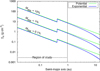 |
Fig. 3 Power law (green line) and exponential tapered (blue line) surface density profiles in the protoplanetary-planetary disk for a total disk mass Mdisk of 0.1, 1, and 10% of the mass of the central object of 0.08 M⊙. The region of study (0.015 < r∕au < 1) is indicated. |
4.4 Contrasting Σ parameterization
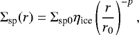
Many authors have also proposed a power-law surface density profile to model protoplanetary disks (e.g., Ciesla et al. 2015; Testi et al. 2016). We therefore compared the model proposed in this work (Eq. (4)) with a power-law density profile,
 (6)
(6)
where r0 and p are equivalent to rc and γ in the exponentially tapered density profile. In Fig. 3 we show the comparison of the two density profiles considering the same initial parameters as we chose to describe Σs(r) (see Sect. 4.2). As an example, we selected three different disk masses Mdisk: 0.1, 1, and 10% of the massof the central object, and we assumed a gas-to-dust ratio of 100 : 1. The power-law profiles do not show significant differences with the exponentially tapered density profiles within our region of study.
5 Numerical model
In this section we describe the treatment of planet formation around an object of 0.08 M⊙ by including a protoplanetary embryo distribution that interacts with the main object. We developed a set of N-body simulations with the well-known mercury code (Chambers 1999) by incorporating tidal and general relativistic acceleration corrections as external forces. Thus the dynamical evolution of protoplanetary embryos was affected not only by gravitational interactions between them and with the star, but also by tidal distortions and dissipation, as well as by general relativistic effects. The stellar contraction and rotational period evolution was included in the code as well as a fixed pseudo-synchronization period for protoplanetary embryos during the 100 Myr integration time of our simulations.
5.1 Tidal model
We followed the equilibrium tide model (Hut 1981; Eggleton et al. 1998) that was rederivated by Bolmont et al. (2011), which considers both the tide raised by the BD on the planet and by the planet on the BD in the orbital evolution of planetary systems. It also takesinto account the spin-up and contraction of the BD. The authors followed the constant time-lag model and assumed constant internal dissipation for the BD and the planets involved. Following the equilibrium tidal model, we incorporated tidal distortions and dissipation terms, considering the tide raised by the star on each protoplanetary embryo and by each protoplanetary embryo on the star and neglected the tide between embryos. Tidal interactions produce deformations on the bodies that in a heliocentric reference frame lead to precession of the argument of periastron ω and a decay in semimajor axis a and eccentricity e, which can be interpreted as distortions and dissipation terms, respectively.
The correction in the acceleration of each protoplanetary embryo produced by the tidal distortion term was taken from Hut (1981) (for an explicit expression, see Beaugé & Nesvorný 2012) and is given by
![Mathematical equation: \begin{equation*} \textbf{f}_{\omega} = -3\frac{\mu}{r^8}\left[k_{2,\star}\left(\frac{M_{\mathrm{p}}}{M_{\star}}\right)R_{\star}^5 + k_{2,\mathrm{p}}\left(\frac{M_{\star}}{M_{\mathrm{p}}}\right)R_{\mathrm{p}}^5\right] \vec{r}, \end{equation*}](/articles/aa/full_html/2020/05/aa37317-19/aa37317-19-eq7.png) (7)
(7)
where r is the position vector of the embryo with respect to the central object, k2,⋆ = 0.307 and k2,p = 0.305 are the potential Love numbers of degree 2 of the star and the embryo, respectively (Bolmont et al. 2015), μ = G(M⋆ + Mp), G is the gravitational constant, and M⋆, R⋆, Mp, and Rp are the masses and radius of the star and the protoplanetary embryo under the approximation that these objects can instantaneously adjust their equilibrium shapes to the tidal force and considering only distoritions up to the second-order harmonic (Darwin 1908).
The evolution of R⋆ was taken from the models of Baraffe et al. (2015), and the value of Rp of each protoplanetary embryo was calculated by considering each of them as a spherical body with a fixed volume density ρ = 5 gr cm−3.
The timescale associated with the tidal dissipation term was calculated based on the work of Sterne (1939) by considering the stellar and embryo tide, and it is given by
 (8)
(8)
with ![Mathematical equation: $f(e) = (1-e^2)^{-5}[1 + (3/2)e^2 + (1/8)e^4]$](/articles/aa/full_html/2020/05/aa37317-19/aa37317-19-eq9.png) . The acceleration correction of each protoplanetary embryo induced by the tidal dissipation term, which produces a and e decay, was obtained from Eggleton et al. (1998). After some algebra, this equals the expression from Beaugé & Nesvorný (2012),
. The acceleration correction of each protoplanetary embryo induced by the tidal dissipation term, which produces a and e decay, was obtained from Eggleton et al. (1998). After some algebra, this equals the expression from Beaugé & Nesvorný (2012),
![Mathematical equation: \begin{align*} \textbf{f}_{\textrm{ae}} = & -3\frac{\mu}{r^{10}} \left[ \frac{M_{\textrm{p}}}{M_{\star}} k_{2,\star} \Delta {t}_{\star} R_{\star}^{5}\left(2\vec{r}(\vec{r} \cdot \vec{v}) + r^{2}(\vec{r} \times \Omega_{\star} + \vec{v})\right)\right]\\ \qquad\ \ -3\frac{\mu}{r^{10}} \left[\frac{M_{\star}}{M_{\textrm{p}}}k_{2,\textrm{p}} \Delta {t}_{\textrm{p}} R_{\textrm{p}}^{5} \left(2\vec{r}(\vec{r}\cdot\vec{v}) + r^{2}(\vec{r} \times \Omega_{\textrm{p}} + \vec{v})\right)\right], \end{align*}](/articles/aa/full_html/2020/05/aa37317-19/aa37317-19-eq10.png) (9)
(9)
where v is the velocity vector of the embryo, and Δt⋆ and Δtp are the time-lag model constants for the star and the protoplanetary embryo, respectively. The factors k2,⋆ Δt⋆, and k2,pΔtp are related to the dissipation factors by
 (10)
(10)
with the dissipation factor for each protoplanetary embryo σp = 8.577 × 10−50g−1cm−2s−1, the same dissipation factor as estimated for the Earth (Neron de Surgy & Laskar 1997), and the dissipation factor of the central object is σ⋆ = 2.006 × 10−60g−1cm−2s−1 (Hansen 2010).
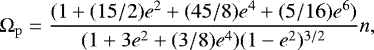
In the constant time-lag model, in which the time-lag constant Δt⋆ is independentof the tidal frequency, the rotation of the companions leads to pseudo-synchronization (Hut 1981; Eggleton et al. 1998). In preliminary simulations, Leconte et al. (2010); Bolmont et al. (2011, 2013) verified that a planet reaches the pseudo-synchronization very quickly in its evolution. For a planet, being at pseudo-synchronization means that its rotation tends to be synchronized with the orbital angular velocity at periastron, where the tidal interactions are stronger (Hut 1981). As in Bolmont et al. (2011), we fixed each protoplanetary embryo at pseudo-synchronization (Hut 1981) in each time-step of our simulations as
 (11)
(11)
where Ωp is the rotational velocity of the protoplanetary embryo.
If e = 0, then the embryo is in perfect synchronization, thus Ωp = n and only the tide of the central object remain. When e is small, the tide of the main object dominates and determines the evolution of the embryo: if the embryo is located beyond rcorot, then  so that the embryo is pushed outward, and if it is inside,
  so that the embryo is pulled inward. On the other hand, when e is high, the embryo tide will prevail. In this case, the embryo is pulled inward. This is always true because for a body in pseudo-synchronization, the body tide always acts to decrease the orbital distance (Leconte et al. 2010).
The rotational velocity Ω⋆ of the main object was calculated following the tidal model proposed by Bolmont et al. (2011), who integrated its evolution as affected by its contraction and the influence of orbiting planets. They calibrated their results with a set of observationally determined Ω⋆ for VLMS and BDs at different ages from Herbst et al. (2007). Thus the evolution of Ω⋆ can be expressed as
![Mathematical equation: \begin{equation*} \Omega_{\star}(t)=\Omega_{\star}(t_0)\left[\frac{r_{\mathrm{gyr}}^2(t_0)}{r_{\mathrm{gyr}}^2(t)}\left(\frac{R_{\star}(t_0)}{R_{\star}(t)}\right)^{2}\times {\textrm{exp}}\left(\int_{t_0}^{t}f_{\textrm{t}} \textrm{d}t\right)\right]\end{equation*}](/articles/aa/full_html/2020/05/aa37317-19/aa37317-19-eq16.png) (12)
(12)
(e.g., Bolmont et al. 2011), where  is the square of thegyration radius, defined as
  , with I⋆ the moment of inertia of the main object (Hut 1981). The function ft is given by
 (13)
(13)
If we were to consider  and R⋆ as constant values (Bolmont et al. 2011), then
![Mathematical equation: \begin{equation*}f_{\mathrm{t}}=-\frac{\gamma_{\star}}{t_{\mathrm{dis},\star}}\left[No1(e) - \frac{\Omega_{\star}}{n}No2(e)\right] ,\end{equation*}](/articles/aa/full_html/2020/05/aa37317-19/aa37317-19-eq21.png) (14)
(14)
with  , where h is the orbital angular momentum, tdis,⋆ is the dissipation timescale of the central object (see below), and the functions No1(e) and No2(e) are dependent on the eccentricity of the planetary companion, which is given by
 (15)
(15)
When only terrestrial planets are considered to orbit the host object, then ft is small andthe substellar object rotation period is mainly determined by the conservation of angular momentum, that is, by the initial rotation period (Bolmont et al. 2011). We therefore numerically integrated Eq. (12) independently of the dynamics of the planetary system. We considered that the radius R⋆ evolves according to the structure and atmospheric models from Baraffe et al. (2015), but we fixed its value for each time-step of our integration, which was small enough to be considered constant in order to simplify the integration and be able to use Eq. (14). We also assumed one Earth-like planet to orbit the main object with random initial values for e and a inside our region of study. From the different orbital elements initially given to the Earth-like planet, we verified that the evolution of Ω⋆ was mainly determined by the evolution of the substellar object and was similar to the evolution achieved by Bolmont et al. (2011). In Fig. 4 we show the resulting evolution of the rotational period and the corresponding R⋆ in a period from 1 to 100 Myr.
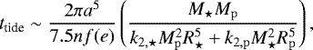
The dissipation timescales for eccentric orbits are determined from the secular tidal evolution of a and e (see Hansen 2010; Bolmont et al. 2011, 2013) as ta and te, respectively,by
![Mathematical equation: \begin{equation*} \begin{split} \frac{1}{t_{\textrm{a}}}=\frac{1}{a} \frac{\textrm{d}a}{\textrm{d}t} = - \frac{1}{t_{\textrm{dis,p}}} \left[Na1(e) - \frac{\Omega_{\textrm{p}}}{n}Na2(e) \right] \\ - \frac{1}{t_{\mathrm{dis},\star}} \left[Na1(e) - \frac{\Omega_{\star}}{n}Na2(e) \right] \end{split} \end{equation*}](/articles/aa/full_html/2020/05/aa37317-19/aa37317-19-eq24.png) (16)
(16)
![Mathematical equation: \begin{equation*} \begin{split} \frac{1}{t_{\textrm{e}}}=\frac{1}{e} \frac{\textrm{d}e}{\textrm{d}t} = & - \frac{9}{2t_{\textrm{dis,p}}} \left[Ne1(e) - \frac{11}{18} \frac{\Omega_{\textrm{p}}}{n}Ne2(e)\right], \\ &- \frac{9}{2t_{\mathrm{dis},\star}}\left[ Ne1(e) - \frac{11}{18} \frac{\Omega_{\star}}{n}Ne2(e) \right]. \end{split} \end{equation*}](/articles/aa/full_html/2020/05/aa37317-19/aa37317-19-eq25.png) (17)
(17)
Here tdis,p and tdis,⋆ are the dissipation timescales for circular orbits for the embryo and the main object, respectively, and Na1, Na2, Ne1, and Ne2 are factors that take place in eccentric orbits and are defined by
![Mathematical equation: \begin{align*} & t_{\textrm{dis,p}} = \frac{1}{9} \frac{M_{\textrm{p}}}{M_{\star}(M_{\textrm{p}} + M_{\star})} \frac{a^8}{R_{\textrm{p}}^{10}} \frac{1}{\sigma_{\textrm{p}}},\nonumber\\[3pt] & t_{\mathrm{dis},\star} = \frac{1}{9} \frac{M_{\star}}{M_{\textrm{p}}(M_{\textrm{p}} + M_{\star})} \frac{a^8}{R_{\star}^{10}} \frac{1}{\sigma_{\star}},\nonumber\\[3pt] & Na1(e) = \frac{1 + (31/2)e^{2} + (255/8)e^{4} + (185/16)e^{6} + (25/64)e^{8}}{(1-e^{2})^{15/2}},\nonumber\\[3pt] & Na2(e) = \frac{1 + (15/2)e^{2} + (45/8)e^{4} + (5/16)e^{6}}{(1-e^{2})^{6}},\nonumber\\[3pt] & Ne1(e) = \frac{1 + (15/4)e^{2} + (15/8)e^{4} + (5/64)e^{6}}{(1-e^{2})^{13/2}},\nonumber\\[3pt] & Ne2(e) = \frac{1 + (3/2)e^{2} + (1/8)e^{4}}{(1-e^{2})^{5}}. \end{align*}](/articles/aa/full_html/2020/05/aa37317-19/aa37317-19-eq26.png) (18)
(18)
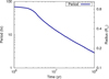 |
Fig. 4 Rotation period evolution of an object of 0.08 M⊙ based on Bolmont et al. (2011) associated with its radius contraction. The radius evolution is taken from Baraffe et al. (2015). |
5.2 General relativistic effect
The important effect derived from General Relativity theory (GRT) on the dynamic of planetary systems is the precession of ω (Einstein 1916). In our case, we considered that only the main object contributes with relevant corrections. As we worked in the reference frame of the star, the associated correction in the acceleration of the embryo is
![Mathematical equation: \begin{equation*} \textbf{f}_{\mathrm{GR}} = \frac{GM_{\star}}{r^3c^2}\left[\left(\frac{4GM_{\star}}{r} - \vec{v}^2\right)\vec{r}+4(\vec{v}.\vec{r})\vec{v}\right],\end{equation*}](/articles/aa/full_html/2020/05/aa37317-19/aa37317-19-eq27.png) (19)
(19)
with c the speed of light. Eq. (19) was proposed by Anderson et al. (1975), who worked under the parameterize post-Newtonian theories. The authors obtained a relative correction associated with two parameters β and γ, which are equal to unity in the GRT case. This expression has been used in several works that included relativistic corrections (e.g., Quinn et al. 1991; Shahid-Saless & Yeomans 1994; Varadi et al. 2003; Benitez & Gallardo 2008; Zanardi et al. 2018). The timescale associated with the precession of the longitude of periastron is given by
 (20)
(20)
5.3 Test simulations
We made a set of N-body simulations in order to test the agreement between the external forces that we incorporated in the MERCURY code and the timescale associated with them. To test the precession of ω, we developed two simulations: one that included the tidal distortion term, and another that included the GR correction. In Fig. 5 we show the apsidal precession timescale of a planet with 1 M⊕ orbiting a 1 Myr substellar object of 0.08 M⊙ with initial values a = 0.01 au and e = 0.1 for the two simulations we made. Our results show that the apsidal precession of 360° is completed in 14 750 and 3060 yr, respectively, which agrees with the time predicted by the timescales associated with each correction term in Eqs. (20) and (8). These timescale values depend on the physical parameters of the protoplanetary embryos and the substellar object, as well as on the initial orbital elements. For instance, if the protoplanets are smaller than Earth in mass and radius, then the relativistic effect is more relevant than the tidal distortion regarding the precession of ω.
To test the analytic expressions for the tidal dissipation with the timescales of e and a decay, we developed a N-body simulation that includes the dissipation term. Our aim was to compare our results with those obtained by Bolmont et al. (2011), who used the analytic tidal model. In their work, they represent the evolution of a, e, and the rotation period of a planet of 1 M⊕ evolving around a BD of 0.04 M⊙. We chose as initial values a = 0.017242 au and e = 0.744. The semimajor axis we selected represents aswitch, that is, the one that determines the behavior of the protoplanet and separates inward migration and crash from inward migration but survival of the protoplanet or outward migration.
In Fig. 6 we show the evolution of a, e, and the pseudo-synchronization period Pp of a 1 M⊕ planet around an evolving 0.04 M⊙ BD. In the middle panel, we also show the rcorot evolution, while in the bottom panel we include the rotation period of the BD, P⋆. First, as P⋆ > Pp, the planet moves inward of the central object. Under this condition, even tough a = rcorot, the orbit is not circular and the planet continues to move inward. When P⋆ = Pp, the orbit is circular and then Ωp = n, which means that this time when a = rcorot, the planet starts to move outward because P⋆ < Pp.
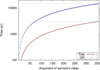 |
Fig. 5 Apsidal precession due to tidal distortion (solid red line) and GR effects (dotted blue line) in a system composed of a 1 M⊕ planet around a 0.08 M⊙ BD with initial a = 0.01 au and e = 0.1. In this example, the argument of periastron completes an orbit in ~14 750 yr when is affected by GR and in ~3060 yr when is affected by tidal distortion. |
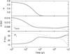 |
Fig. 6 Evolution of e, a, and the pseudo-synchronization period of a 1 M⊕ around a 0.04 M⊙ BD. Solid lines indicates the results considering the initial orbital elements from Bolmont et al. (2011). The dashed lines indicate the evolution of rcorot (middle panel) and the rotational period of the BD, P⋆ (bottom panel). |
5.4 N-body simulations
We performed 20 N-body simulations using the modified version of the MERCURY code. We developed 10 simulations for scenario S1 and 10 simulations for scenario S2, as explained in Sect. 4.3. We also ran 10 simulations for each scenario described above using the original version of the MERCURY code, without external forces, in order to evaluate the relevance of tidal and general relativistic effects.
5.4.1 Protoplanetary embryo distributions
For using mercury code, it is necessary to give physical and orbital parameters for the protoplanetary embryos. We modeled the initial mass distributions of embryos as a function of the radial distance from the central object, which are initial conditions for our numerical simulations. The initial spatial distribution of protoplanetary embryos was computed following Eq. (4), considering a distance range 0.015 < r∕au < 1 and defining 1 Myr as the initial time. We considered that at this age, the gas has already been dissipated from the disk.
Even though we are aware of the existence of a number of BDs that still accrete gas from their disks up to ~ 10 Myr (references, e.g., in Pascucci et al. 2009; Downes et al. 2015), incorporating the gas component is beyond the scope of this work, which reproduces the BDs that are not observed to show gas signatures at ~ 1 Myr, however. We calculated the mass of each protoplanetary embryo Mp considering that at the initial time, they are at the end of the oligarchic growth stage, having accreted all the planetesimals in their feeding zones (Kokubo & Ida 2000) by
 (21)
(21)
where ΔrH is the orbital separation between two consecutive embryos in terms of their mutual Hill radii rH, with Δ an arbitraryinteger number, given by
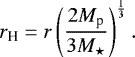 (22)
(22)
By replacing Eqs. (4) and (22) in Eq. (21), we obtain an expression for the mass of each protoplanetary embryo as a function of the radial distance in the disk mid-plane r, which is given by
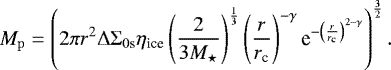 (23)
(23)
We located our first embryo at the inner radii of our region r1 = 0.015 au. Then we calculated its mass using Eq. (23). For the remaining embryos, we propose a separation of 10 rH by fixing Δ = 10 (Kokubo & Ida 1998).
Thus we calculated the initial positions ri+1 and masses Mp,i+1 for the embryos by
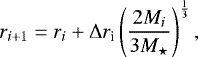 (24)
(24)
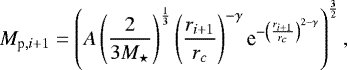 (25)
(25)
for i = 1, 2, etc. with 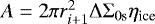 .
.
Using Eqs. (24) and (25), we derived the initial distributions of masses of the protoplanetary embryos as a function of the radial distance, which represents the semimajor axis, from the central object for scenarios S1and S2. In Fig. 7 we illustrate the two distributions. S1 has a distribution of 224 embryos with a total mass MpT ~ 0.25 M⊕ located in the region of study. Two hundred and ten of them are distributed in the inner region up to the snow line, with a total mass ~ 0.06 M⊕, while the remaining 14 embryos are distributed beyond the snow line and have a total mass ~ 0.19 M⊕. S2 has a distribution of 74 embryos that are located in the region of study with a total mass MpT ~ 3 M⊕. Sixty-nine of them are distributed in the inner region up to the snow line, with a total mass ~ 0.72 M⊕, while the remaining 5 embryos have a total mass of ~ 2.25 M⊕ and are placed beyond the snow line up to 1 au.
We considered lower values than 0.02 for the initial eccentricities and 0.5° for the initial inclinations. The orbital elements, argument of periastron ω, longitude of the ascending node Ω, and mean anomaly M were determined randomly at the beginning of the simulations. They were between 0° and 360° from a uniform distribution for each protoplanetary embryo.
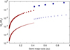 |
Fig. 7 Initial embryo distributions of masses as a function of their initial location given by their semimajor axis for S1 (circles) and S2 (stars). Blue represents the water-rich population (50% water in mass), and red represents the bodies with the lowest amount of water in mass (0.01%). |
5.4.2 N-body code: characterization
To develop our simulations, we chose the hybrid integrator, which uses a second-order symplectic algorithm to treat interactions between objects with separations greater than 3 Hill radii, and we selected the Bulirsch-Stöer method to resolve closer encounters. The collisions were treated as perfectly inelastic, conserving the mass and the corresponding water content of protoplanetary embryos. We considered that a body is ejected from the system when it reaches a distance a > 100 au.
We adopted a time step of 0.08 days, which corresponds to 1∕30 th of the orbital period of the innermost body in the simulations. In order to avoid any numerical error for small-perihelion orbits, we assumed R⋆ = 0.004 au, which corresponds to the maximum value of the radius of the central object.
All simulations were integrated over 100 Myr, which is a standard time for studying the dynamical evolution of planetary systems. Because of the stochastic nature of the accretion process between the protoplanets and eventually with the main object, we remark that it is necessary to carry out a set of N-body simulations. In this case, we performed ten simulations for each scenario, which required a mean CPU time of six months on 3.6 GHz processors.
6 Results
In this section we present the resulting planetary systems of the simulations in scenarios S1 and S2. We compare the resulting planets from simulations that included tidal and GR effects with those from simulations that neglected these effects to test their relevance in the formation of rocky planets. In particular, we focus our analysis on the population that is located close to the central object.
6.1 Planetary architectures
Our simulations predict a diversity of final planetary system architectures at 100 Myr regarding all the simulations made in both scenarios. Figure 8 shows the final location of the resulting planetary systems of each simulation in scenario S1 for the final masses and fraction of water in mass. The planetary masses are between 0.01 M⊕ and 0.12 M⊕ (this is approximately the mass of the Moon and Mars, respectively) and the fraction of water in mass is between 0.01 and 50%. The left panel shows the planetary architectures from simulations that included tidal and GR effects, and the right panel presents their counterparts in the simulations that neglect these effects. In both panels, the IHZ of the system at 100 Myr and at 1 Gyr overlap. In Fig. 9 we show the resulting architectures of the simulations for scenario S2. The resulting planets have a range of masses between 0.2 M⊕ and 1.8 M⊕ and a percentage of water in mass between 0.01 and 50%.
The main difference we found is the close-in planet population that survived in the simulations that included tidal and GR effects, which did not survive in the simulations that neglected these effects. This becomes more relevant in S1, where the protoplanetary embryos involved were an order of magnitude less massive than in S2.
In simulations S2, the embryos involved suffered stronger gravitational interactions between them than those from S1 because they are more massive bodies. Therefore they generate more excitation in the system, allowing some embryos to collide with the central object and to be ejected from the system. These interactions became more relevant than tidal and GR effects for the population of very close-in bodies in S2. This is supported by the percentage of embryos that collided with the central object or were ejected from the system (reached a > 100 au), as shown in Fig. 10. The percentage is given over the initial amount of embryos in each scenario of work: 224 embryos in S1, and 74 embryos in S2. The number of bodies that either collided with the central object or were ejected fromthe system in S2 is much higher than in S1 because the system is more highly excited. Moreover, the simulations that included tidal and GR effects reduced the collisions of embryos with the central object and had almost no effect on the ejection of embryos because at long distances from the central object, tidal effects became irrelevant.
By compacting all the resulting planetary systems in Fig. 11, we represent their distribution in a for their masses for S1 and S2. The IHZ at 100 Myr and at 1 Gyr overlap as well. The surviving population of close-in bodies has low masses and mainly results from simulations with tidal and GR effects from S1. This shows that the relevance of tidal and GR effects also depends on the mass of the bodies that are involved in the simulations.
Figure 12 shows the eccentricities of the resulting planets as a function of their semimajor axis for S1 and S2. Low-mass and close-in planets that survived while external effects were included appear to have eccentricities values greater than zero. This is because the many gravitational interactions between embryos produce excitation in their orbital parameters, and the timescale for eccentricity damping is far longer (approximately some billion years) than the integration time of our simulations. As we discussed in previous sections, the tidal effects added in our simulations affect the distribution of eccentricities and the semimajor axis of the resulting planets, but the long decay timescales prevent us from seeing the damping in e at this point. Nevertheless, the e damping will be efficient by the time the central object reaches 1 Gyr for the planets that remain located close in to the central object, where the IHZ will be located by that time.
Our results strongly suggest that a formation scenario that includes tidal and GR effects is more realistic for planet formation at the substellar mass limit. Although GR corrections are relevant during planet formation, the tidal effects are mor important to map more realistic orbits and therefore more realistic encounters between embryos. These effects play a primary role in the survival of an in situ population. However, when the masses of the bodies involved increase (like in S2), tidal effects became less relevant than the gravitational interactions between them (see Sect. 7).
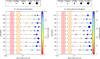 |
Fig. 8 Distribution of the resulting planet locations in the region of study in each simulation for scenario S1. Planets were distinguished by mass and fraction of water in mass. The masses of the resulting planets are shown at the top of each graphic. The range is between 0.01 M⊕ and 0.12 M⊕ (this is approximately the mass of the Moon and Mars, respectively). The fraction of water in mass is presented in color-scale and is assigned to each body as a percentage between 0.01 and 50%. Left panel: resulting planets from simulations in which tidal and GR effects are included during the integration time. Right panel:planets from simulations that neglected these effects. The cream band represent the IHZ at 100 Myr, and the pink band shows the IHZ at 1 Gyr. |
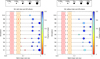 |
Fig. 9 Distribution of the resulting planet locations in the region of study in each simulation for scenario S2. The mass range of the resulting planets is between 0.2 M⊕ and 1.8 M⊕. The color characterization is the same as in Fig. 8. |
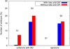 |
Fig. 10 Percentage of embryos that collided or were ejected from the system during the integration time of each scenario. Blue bars correspond to embryos from simulations that included tidal and GR effects, and red bars represent embryos from simulations that neglected these effects. |
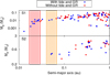 |
Fig. 11 Distribution in mass of the resulting planets for their semimajor axis at 100 Myr in S1 (top panel) and S2 (bottom panel). Blue dots represent the planets from simulations that included tidal and GR effects, while red dots represent those from simulations that neglected these effects. The pink band represents the location of the IHZ at 1 Gyr, while the cream band represents its location at 100 Myr. |
6.2 Water mass fraction
The two scenarios show a diversity in the fraction of water in mass, but the resulting planets inside a < 0.1 au always conserved this initial fraction of water in mass. We assumed this to be 0.01% of the mass of the embryos that are located inside the snow line at the beginning of the simulations.
For S1, planets at a > 0.1 au present a range in percentage of water in mass that is between 10 and 35% for planets with a semimajor axis 0.1 < a∕au < 0.42, and it is between 35 and 50% for planets with0.42 < a∕au < 1. The outer water-rich planets maintain their high content of water in mass, and an intermediate population of water-rich resulting planets appears close to the location of the snow line.
For S2, planets at a > 0.1 au present a high mass percentage of water, between 35 and 50%. Embryos located outside the snow line either have suffered impacts of other water-rich bodies or have been ejected from the system. No intermediate water-rich population as in S1 evolved. In order to explain the origin of the resulting distribution of water of the surviving planets in our region of study, in the next section we analyze their whole collisional history.
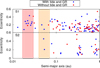 |
Fig. 12 Orbital distribution of the resulting planets regarding their location in the system and eccentricity in S1 (top panel) and S2 (bottom panel). Colors are as in Fig. 11. |
6.3 Collisional history
During the first 100 Myr of planet formation that we studied in our simulations, embryos had gravitational interactions in the form of encounters and collisions among them. From the initial location in the system, each embryo can interact with others that have different orbital and physical parameters in its gravitational influence zone. The N-body code treats all collisions as perfectly inelastic. After two bodies collide, the resulting body therefore is a merger of the initial two.
From the previous analysis of the final distributions of the resulting planets and their final fraction of water in mass, we can distinguish different subregions in which the collisional history of the resulting planets can be studied: an inner region of planets that are finally located at a < 0.1 au, an intermediate region, between 0.1 < a∕au < 0.42, and an outer region beyond the snow line, between 0.42 < a∕au < 1.
Figure 13 shows the collisional history of all the resulting planets of S1 when tidal and GR effects are includedand when these effects are neglected. Each peak in the lines represents the initial location of the embryo thatcollided with the resulting planet and the percentage of mass that it added to the planet after the perfect collision. In the inner region the resulting planets collided with embryos that were initially located at a < 0.35 au, all located inside the snow line, which means that they preserve the initial fraction of water in mass. In the intermediate region, planets accreted embryos that were initially located between 0.05< a∕au < 0.88 and between 0.05 < a∕au < 0.95, which explains the intermediate range of water in mass after collision with embryos inside and outside the snow line. Finally, in the outer region, planets collided with embryos that were initially located between 0.2 < a∕au < 0.95 and 0.22< a∕au < 0.95. In this outer region, even though the resulting planets suffered collisions with embryos that were distributed in a wide range of thesystem, only a few planets that were located inside the snow line collided with these planets and thus maintained a huge fraction of water in mass. It is important to remark that the close-in population located at a < 0.1 au did not collide with other embryos beyond this semimajor axis when tidal effects were included in the simulations.
On the other hand, Fig. 14 shows the collisional history of the resulting planets of S2 when tidal and GR effects are included and when these effects are neglected. In this case, in the inner-region planets collided with embryos that were initially located at a< 0.36 au and a < 0.22 au. In the intermediate region, planets accreted embryos that were initially located between 0.06< a∕au < 0.72 and 0.07< a∕au < 0.91. Finally, in the outer region, planets collided with embryos that were initially located at 0.17< a∕au < 0.72 and 0.097 < a∕au < 0.72. In S2, planets in the intermediate and outer region accreted material from a similar region, with a few embryos initially located inside the snow line. Thus all these planets retained a huge amount of water in mass. In this case, the three planets that survived with at a < 0.1 au did not collide with other embryos beyond this semimajor axis as happened in S1 when tidal effects were included in the simulations.
The collisional history of the resulting planets explains their final masses and the fraction of water in mass. Moreover, it allows us to conclude that the close-in surviving population that was most affected by tidal effects only suffered collisions with the embryos that were initially located close in.
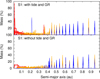 |
Fig. 13 Collisional history of the resulting planets from the simulations in S1 in which tidal and GR effects are included (top panel) and in which these effects are neglected (bottom panel). Each jump in semimajor axis indicates the initial location of the embryo that collided with the resulting planets that increased their masses by a given percentage after the perfect merger. The red lines indicate the history of the resulting planets that are finally located at a < 0.1 au, the orange lines show planets located at 0.1 < a∕au < 0.42, and the blue lines represent planets located at 0.42 < a∕au < 1. |
6.4 Close-in population: potentially habitable planets
We focus our analysis on the close-in bodies that survived in the simulated planetary systems. We gave physical and orbital parameters of those bodies candidates to be potentially habitable planets.
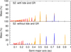 |
Fig. 14 Collisional history of the resulting planets from the S2 simulations in which tidal and general relativistic effects are included (top panel) and in which these effects are neglected (bottom panel). Colors are the same as in Fig. 13. |
6.4.1 Characterization
Inside the location of the IHZ at 100 Myr (final time of simulations), two planets in S1 remained when tidal and GR effects were included in the simulations and only one planet remained when these effects were excluded from the simulations regarding their semimajor axis. On the other hand, in S2 two planets remained in the IHZ when external effects were included and no candidate survived when these effects were excluded from the simulations. Moreover, when we consider the value of the eccentricity and calculate the periastron distance (q) and apastro distance (Q) of these planets, only one planet remained inside the IHZ in a, q, and Q in S1 and 1 in S2 when tidal and general relativistic effects were considered in the simulations.
In Sect. 3 we discussed the behavior of the IHZ around very low mass stars that are located close to the star and evolve toward a smaller radius as the star evolves with time. We therefore extended our analysis to bodies that ended up closer in to the central object, in particular, inside the location of the IHZ at 1 Gyr. The S1 alone generated such a close-in body population: nine planets when tidal and GR effects were incldued, and only one planet when these effects were neglected in the simulations regarding their semimajor axis. Even though we do not have the orbital parameters at 1 Gyr, it is expected that the eccentricities of these planets are small enough for them to remain in the IHZ at 1 Gyr in S1 (see Sect. 5). In Table 1 we present some physical parameters of the planets that remained in the IHZ at 100 Myr or at 1 Gyr in both scenarios. When tidal and GR effects are included in the simulations, S1 is the most favorable scenario to allow these candidates of potentially habitable planets (see Sect. 7 for further discussion.)
6.4.2 Mass accretion history
All the close-in population that we consider as candidates for potentially habitable planets had many collisions during the integration time of our simulations. All of them were targets of many impacts. We show in Fig. 15 the number of collisions of all the IHZ candidates at 100 Myr and 1 Gyr. In S1, all the resulting planets received more than 50 impacts and a maximum of 160 impacts, and 50% of the total received more than 100 impacts when tidal and GR effects were included, while the planets received 70 and 127 impacts when these effects were neglected. In S2, one of the planets received 29 impacts and the other almost 70 impacts when tidal and GR effects were included. Each impact corresponds to a collision with another embryo of the simulation. In S1 more impacts are allowed because the total number of embryos is much higher (224 in total) than in S2 (74 in total). In any case, all the candidate planets collided with between 25 and 50% of the total number of embryos during the first 100 Myr of their evolution.
Table 1 shows that all the planets inside the IHZ conserved their initial fraction of water in mass because all the impacts that they suffered came from embryos that were located inside the snow line of the system. Figure 16 shows the location on the semimajor axis of each embryo that collided with one IHZ candidate, related to the percentage of mass that the candidate obtained after each collision in S1 with tide and GR, in S2 without tide and GR, and in S2 with tide and GR. This figure is a zoom of Figs. 13 and 14 for the planets located in the two determined IHZ.
The impacts that each body suffered during the integration time always produced an increase in mass because the N-body code we used to develop the simulations considers all collisions as completely inelastic, so that every time a collision between embryos occurs, it ends in a perfect merger (see Sect. 7). In Fig. 17 we show the evolution in mass of each IHZ candidate planet and its fraction of mass. Each step in the curves represents the mass or fraction of mass, respectively,that is gained by the IHZ candidate planet after each collision. There is no difference between candidate planets that were finally located in the IHZ at 100 Myr and 1 Gyr in each scenario with respect to the mass accretion history.
Potentially habitable planets from both scenarios when tidal and GR effects are included in the simulations (S1t and S2t) and when these effects are neglected in the case of S1 (S1wt).
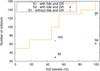 |
Fig. 15 Cumulative collisions between the resulting planets that survived inside the IHZ at 100 Myr and at 1 Gyr for S1 with tide and GR (orange line), S1 without considering tide or GR (cyan dots), and S2 with tide and GR. |
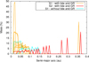 |
Fig. 16 Initial location of each embryo that collided with planets that survived inside the IHZ at 100 Myr or 1 Gyr related to the percentage of mass that the candidate planet obtained after each collision in S1 with tide and GR (orange curves), in S2 without tide and GR (cyan curves), and in S2 with tide and GR (red curves). |
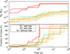 |
Fig. 17 Evolution of the mass (top panel) and its fraction with respect to the final mass (bottom panel) of the resulting planets thatsurvived inside the IHZ at 100 Myr (solid lines) and 1 Gyr (dotted lines) in S1 with tide and GR (orange curves), in S2 without tide and GR (cyan curves), and in S2 with tide and GR (red curves). |
7 Conclusions and discussions
We studied the rocky planet formation around a star close to the substellar mass limit using N-body simulations that included tidal and GR effects and did not include the effect of gas in the disk. Our aim was to evaluate the relevance of tidal effects following the equilibrium tidal model during the formation and evolution of the system and to improve the accuracy in the calculation of the orbit of the protoplanetary embryos by considering GR effects.
The equilibrium tide model we used is based on the assumption that when a star suffers tidal disturbance from a companion body, it instantly adjusts to hydrostatic equilibrium (Darwin 1879). A more general approach must include the dynamical tide model for a more reliable description of the very high eccentricity orbits, as shown by Ivanov & Papaloizou (2011) and references therein. As shown in Fig. 10, in simulations that do not include tides, 7 and 20% of the embryos collide with the central star in S1 and S2, respectively, because of their high eccentricity. When tides are included through the equilibrium model, these fractions change to 1 and 16%, respectively. New simulations that include the dynamical tide model are needed in order to explore the possible change in these fractions, which we expect to occur toward lower values because the tidal damping produced by this model is stronger.
Using a different model for close-in bodies, Makarov & Efroimsky (2013) found non-pseudo-synchronization in the rotational periods for terrestrial planets and moons. In our case, we adopted the pseudo-synchronization to maintain consistency with the Hut (1981) model that we adopted for the N-body simulations because the hypothesis of pseudo-synchronization is a direct consequence of the constant time-lag model (Darwin 1879; Hut 1981; Eggleton et al. 1998). A comparative analysis of our results with those from other treatments as well as the self-consistent inclusion of the rotational evolution of embryos is beyond the goals of this work.
Because of the current uncertainties in the determination of disk masses, the simulations were performed for two different scenarios S1 and S2, which basically differ in the initial mass of solid material in the disk, ~ 3 M⊕ and ~ 30 M⊕, respectively. These values roughly represent the corresponding upper and lower limits of the disk mass for stars close to the substellar mass limit.
The resulting planets have masses between 0.01 < m∕M⊕ < 0.12 in scenario S1 and 0.2 < m∕M⊕ < 1.8 in scenario S2. Even though we used lower values for the disk mass than those from Payne & Lodato (2007), we found the same correlation between the resulting planet masses and the initial amount of solid material in the disk. When the disk mass increases, more massive planets could be formed.
When tidal and general relativistic effects are included, a close-in planetary population located at a < 0.07 au in scenario S1 survived in all the simulations, while in the more massive scenario S2, embryos suffered stronger gravitational interaction and the formation of this close-in population occurred only in two of the ten simulations. S1 therefore is the most favorable scenario for generating close-in planets. Then, we found that tidal and general relativistic effects are relevant during the formation and evolution of rocky planets around an object at the substellar mass limit, in particular when the protoplanetary embryos involved are low-mass bodies. Our work together with the model developed by Bolmont et al. (2011, 2013, 2015) shows that tidal effects in both the formation and later evolution of such systems are required.
The close-in population resulted from a large number of collisions among the protoplanetary embryos, which was treated in our simulations as perfectly inelastic collisions. This gives upper limits on the final mass value and water content for the resulting planets. This shows why it is necessary to reproduce the simulations using an N-body code that includes fragmentation during collisions, which can decrease the final masses of the resulting planets considerably, as shown by Chambers (2013); Dugaro et al. (2019).
The close-in population we found is of particular interest because it is located inside the evolving IHZ of the system. We classified a set of 15 close-in bodies as candidates to potentially habitable planets based on their semimajor axes and eccentricities. A complete analysis of their probability of being habitable planets considering additional constraints (e.g., Martin et al. 2006)is beyond the scope of this work.
Our model presents an important improvement in the scenario of rocky planet formation at the substellar mass limit by including tidal and general relativistic effects. We stress that even tough Coleman et al. (2019) did not incorporate these effects in their simulations of planet formation around Trappist 1, they showed the relevance of considering the gas component of the disk during the first 1 Myr. A more realistic simulation of this scenario of planet formation must therefore clearly include all these effects. A new set of such N-body simulations considering low-mass stars and BDs as central objects with different masses is currently ongoing.
We conclude that tidal and GR effects are relevant during rocky planet formation at the substellar mass limit because they allow the survival of close-in bodies that are located inside the IHZ. This supports the hypothesis that these systems are important candidates for future searches of life in the solar neighborhood.
Acknowledgements
This work was partially financed by Agencia Nacional de Promoción Científica y Tecnológica (ANPCyT) through PICT 201-0505, and by Universidad Nacional de La Plata (UNLP) through PID G144. We acknowledge the financial support by Facultad de Ciencias Astronómicas y Geofísicas de La Plata (FCAGLP) and Instituto de Astrofísica de La Plata (IALP) for extensive use of their computing facilities. We specially appreciate the kind support and advice from Bolivia Cuevas-Otahola (INAOE, México) during the numerical simulations and Adrián Rodríguez Colucci (UFRJ, Brazil) for his valuable comments. We thank the editor Benoît Noyelles and the anonymous referee for very valuable suggestions which helped improve the presentation of our results.
Appendix A Snow-line location in the substellar regime
The snow-line location corresponds to the radial distance to the central object where water condenses. This occurs when the partial pressure of the protoplanetary disk exceeds the saturation pressure. The exact temperature where this occurs depends on the physical structure of the disk and on the relative abundances of elements, but is expected to be in a range between 140 < T∕K < 170. To determine the snow-line location in a system with a substellar object of a mass 0.08 M⊙ as a primary object, we took the same temperature profile of a disk that radiates as a blackbody as Chiang & Goldreich (1997),
 (A.1)
(A.1)
The parameter α represents the glazing angle at which the starlight strikes the disk. Chiang & Goldreich (1997) considered vertical hidrostatic equilibrium and derived the expression
 (A.2)
(A.2)
where the parameter H represents the height of the visible photosphere above the disk mid-plane, and the factor (H∕a) can be expressed by
 (A.3)
(A.3)
where k is the Boltzman constant and μg is the mass of the molecular hydrogen.
By replacing Eqs. (A.3) in (A.2), we estimated a value of α. We considered then that the snow line is located where the disk reaches a temperature of T(r = rice) = Tice = 140 K. Thus we could estimated the location of the snow line by
 (A.4)
(A.4)
We estimated the location of the snow line at rice = 0.42 au, when the BD is 1 Myr old, that is, the initial time of our simulations. We considered this value fixed in all the simulations. Because we know that T⋆ and R⋆ evolve with time, the location of the snow line would also evolve and continuously approach the star. When we consider that the location of the snow line evolves with time, it might have important consequences for the final amount of water in mass of the resulting planets of the simulations. However, this treatment is beyond the scope of this work.
References
- Anderson, J. D., Esposito, P. B., Martin, W., Thornton, C. L., & Muhleman, D. O. 1975, ApJ, 200, 221 [NASA ADS] [CrossRef] [Google Scholar]
- Andrews, S. M., Wilner, D. J., Hughes, A. M., Qi, C., & Dullemond, C. P. 2009, ApJ, 700, 1502 [NASA ADS] [CrossRef] [Google Scholar]
- Andrews, S. M., Wilner, D. J., Hughes, A. M., Qi, C., & Dullemond, C. P. 2010, ApJ, 723, 1241 [NASA ADS] [CrossRef] [Google Scholar]
- Baraffe, I., Homeier, D., Allard, F., & Chabrier, G. 2015, A&A, 577, A42 [NASA ADS] [CrossRef] [EDP Sciences] [Google Scholar]
- Barclay, T., Pepper, J., & Quintana, E. V. 2018, ApJS, 239, 2 [NASA ADS] [CrossRef] [Google Scholar]
- Barnes, R., Raymond, S. N., Greenberg, R., Jackson, B., & Kaib, N. A. 2010, ApJ, 709, L95 [NASA ADS] [CrossRef] [Google Scholar]
- Barnes, R., Mullins, K., Goldblatt, C., et al. 2013, Astrobiology, 13, 225 [NASA ADS] [CrossRef] [Google Scholar]
- Bastian, N., Covey, K. R., & Meyer, M. R. 2010, ARA&A, 48, 339 [NASA ADS] [CrossRef] [Google Scholar]
- Beaugé, C., & Nesvorný, D. 2012, ApJ, 751, 119 [NASA ADS] [CrossRef] [Google Scholar]
- Benitez, F., & Gallardo, T. 2008, Celest. Mech. Dyn. Astron., 101, 289 [NASA ADS] [CrossRef] [Google Scholar]
- Bolmont, E., Raymond, S. N., & Leconte, J. 2011, A&A, 535, A94 [NASA ADS] [CrossRef] [EDP Sciences] [Google Scholar]
- Bolmont, E., Selsis, F., Raymond, S. N., et al. 2013, A&A, 556, A17 [NASA ADS] [CrossRef] [EDP Sciences] [Google Scholar]
- Bolmont, E., Raymond, S. N., Leconte, J., Hersant, F., & Correia, A. C. M. 2015, A&A, 583, A116 [NASA ADS] [CrossRef] [EDP Sciences] [Google Scholar]
- Chambers, J. E. 1999, MNRAS, 304, 793 [NASA ADS] [CrossRef] [MathSciNet] [Google Scholar]
- Chambers, J. E. 2013, Icarus, 224, 43 [NASA ADS] [CrossRef] [Google Scholar]
- Chiang, E. I., & Goldreich, P. 1997, ApJ, 490, 368 [NASA ADS] [CrossRef] [Google Scholar]
- Ciesla, F. J., Mulders, G. D., Pascucci, I., & Apai, D. 2015, ApJ, 804, 9 [NASA ADS] [CrossRef] [Google Scholar]
- Coleman, G. A. L., Leleu, A., Alibert, Y., & Benz, W. 2019, A&A, 631, A7 [NASA ADS] [CrossRef] [EDP Sciences] [Google Scholar]
- Cumming, A., Butler, R. P., Marcy, G. W., et al. 2008, PASP, 120, 531 [CrossRef] [Google Scholar]
- Darwin, G. H. 1879, Phil. Trans. R. Soc. London, Ser. I, 170, 1 [NASA ADS] [CrossRef] [Google Scholar]
- Darwin, G. H. 1908, Proc. R. Soc. London Ser. A, 80, 166 [NASA ADS] [CrossRef] [Google Scholar]
- Downes, J. J., Román-Zúñiga, C., Ballesteros-Paredes, J., et al. 2015, MNRAS, 450, 3490 [NASA ADS] [CrossRef] [Google Scholar]
- Dugaro, A., de Elía, G. C., & Darriba, L. A. 2019, A&A, 632, A14 [NASA ADS] [CrossRef] [EDP Sciences] [Google Scholar]
- Eggleton, P. P., Kiseleva, L. G., & Hut, P. 1998, ApJ, 499, 853 [NASA ADS] [CrossRef] [Google Scholar]
- Einstein, A. 1916, Annalen der Physik, 354, 769 [NASA ADS] [CrossRef] [Google Scholar]
- Gillon, M., Triaud, A. H. M. J., Demory, B.-O., et al. 2017, Nature, 542, 456 [NASA ADS] [CrossRef] [PubMed] [Google Scholar]
- Grimm, S. L., Demory, B.-O., Gillon, M., et al. 2018, A&A, 613, A68 [NASA ADS] [CrossRef] [EDP Sciences] [Google Scholar]
- Guilloteau, S., Dutrey, A., Piétu, V., & Boehler, Y. 2011, A&A, 529, A105 [NASA ADS] [CrossRef] [EDP Sciences] [Google Scholar]
- Hansen, B. M. S. 2010, ApJ, 723, 285 [NASA ADS] [CrossRef] [Google Scholar]
- Hardegree-Ullman, K. K., Cushing, M. C., Muirhead, P. S., & Christiansen, J. L. 2019, AJ, 158, 75 [NASA ADS] [CrossRef] [Google Scholar]
- Hartmann, L., Calvet, N., Gullbring, E., & D’Alessio, P. 1998, ApJ, 495, 385 [NASA ADS] [CrossRef] [Google Scholar]
- Hayashi, C., & Nakano, T. 1963, Prog. Theor. Phys., 30, 460 [NASA ADS] [CrossRef] [Google Scholar]
- He, M. Y., Triaud, A. H. M. J., & Gillon, M. 2017, MNRAS, 464, 2687 [NASA ADS] [CrossRef] [Google Scholar]
- Heller, R., Jackson, B., Barnes, R., Greenberg, R., & Homeier, D. 2010, A&A, 514, A22 [NASA ADS] [CrossRef] [EDP Sciences] [Google Scholar]
- Hendler, N. P., Mulders, G. D., Pascucci, I., et al. 2017, ApJ, 841, 116 [Google Scholar]
- Henry, T. J. 2004, ASP Conf. Ser., 318, 159 [NASA ADS] [Google Scholar]
- Herbst, W., Eislöffel, J., Mundt, R., & Scholz, A. 2007, in Protostars and Planets V, eds. B. Reipurth, D. Jewitt, & K. Keil (Tucson: University of Arizona Press), 297 [Google Scholar]
- Hojjatpanah, S., Figueira, P., Santos, N. C., et al. 2019, A&A, 629, A80 [NASA ADS] [CrossRef] [EDP Sciences] [Google Scholar]
- Howard, A. W. 2013, Science, 340, 572 [NASA ADS] [CrossRef] [PubMed] [Google Scholar]
- Hut, P. 1981, A&A, 99, 126 [NASA ADS] [Google Scholar]
- Isella, A., Carpenter, J. M., & Sargent, A. I. 2009, ApJ, 701, 260 [NASA ADS] [CrossRef] [Google Scholar]
- Ivanov, P. B., & Papaloizou, J. C. B. 2011, Celest. Mech. Dyn. Astron., 111, 51 [NASA ADS] [CrossRef] [Google Scholar]
- Kasting, J. F. 1988, Icarus, 74, 472 [NASA ADS] [CrossRef] [PubMed] [Google Scholar]
- Kasting, J. F., Whitmire, D. P., & Reynolds, R. T. 1993, Icarus, 101, 108 [NASA ADS] [CrossRef] [PubMed] [Google Scholar]
- Kobayashi, H., Kimura, H., Watanabe, S.-i., Yamamoto, T., & Müller, S. 2011, Earth Planets Space, 63, 1067 [Google Scholar]
- Kokubo, E., & Ida, S. 1998, Icarus, 131, 171 [NASA ADS] [CrossRef] [Google Scholar]
- Kokubo, E., & Ida, S. 2000, Icarus, 143, 15 [NASA ADS] [CrossRef] [Google Scholar]
- Kopparapu, R. K., Ramirez, R., Kasting, J. F., et al. 2013a, ApJ, 765, 131 [NASA ADS] [CrossRef] [Google Scholar]
- Kopparapu, R. K., Ramirez, R., Kasting, J. F., et al. 2013b, ApJ, 770, 82 [NASA ADS] [CrossRef] [Google Scholar]
- Kubas, D., Beaulieu, J. P., Bennett, D. P., et al. 2012, A&A, 540, A78 [NASA ADS] [CrossRef] [EDP Sciences] [Google Scholar]
- Kumar, S. S. 1963, ApJ, 137, 1121 [NASA ADS] [CrossRef] [Google Scholar]
- Leconte, J., Chabrier, G., Baraffe, I., & Levrard, B. 2010, A&A, 516, A64 [NASA ADS] [CrossRef] [EDP Sciences] [Google Scholar]
- Lodders, K. 2003, ApJ, 591, 1220 [NASA ADS] [CrossRef] [Google Scholar]
- Lovis, C., Snellen, I., Mouillet, D., et al. 2017, A&A, 599, A16 [NASA ADS] [CrossRef] [EDP Sciences] [Google Scholar]
- Luhman, K. L. 2012, ARA&A, 50, 65 [NASA ADS] [CrossRef] [Google Scholar]
- Lynden-Bell, D., & Pringle, J. E. 1974, MNRAS, 168, 603 [NASA ADS] [CrossRef] [Google Scholar]
- Makarov, V. V., & Efroimsky, M. 2013, ApJ, 764, 27 [NASA ADS] [CrossRef] [Google Scholar]
- Manara, C. F., Morbidelli, A., & Guillot, T. 2018, A&A, 618, L3 [NASA ADS] [CrossRef] [EDP Sciences] [Google Scholar]
- Martin, H., Albarède, F., Claeys, P., et al. 2006, Earth Moon Planets, 98, 97 [NASA ADS] [CrossRef] [Google Scholar]
- Miguel, Y., Cridland, A., Ormel, C. W., Fortney, J. J., & Ida, S. 2020, MNRAS, 491, 1998 [NASA ADS] [Google Scholar]
- Mohanty, S., Basri, G., Shu, F., Allard, F., & Chabrier, G. 2002, ApJ, 571, 469 [NASA ADS] [CrossRef] [Google Scholar]
- Mordasini, C., Alibert, Y., & Benz, W. 2009, A&A, 501, 1139 [NASA ADS] [CrossRef] [EDP Sciences] [Google Scholar]
- Mulders, G. D., Pascucci, I., & Apai, D. 2015, IAU General Assembly, 22, 2256025 [NASA ADS] [Google Scholar]
- Neron de Surgy, O., & Laskar, J. 1997, A&A, 318, 975 [NASA ADS] [Google Scholar]
- Padoan, P., & Nordlund, Å. 2004, ApJ, 617, 559 [NASA ADS] [CrossRef] [Google Scholar]
- Papaloizou, J. C. B., & Terquem, C. 2010, MNRAS, 405, 573 [NASA ADS] [Google Scholar]
- Pascucci, I., Apai, D., Luhman, K., et al. 2009, ApJ, 696, 143 [NASA ADS] [CrossRef] [Google Scholar]
- Payne, M. J., & Lodato, G. 2007, MNRAS, 381, 1597 [NASA ADS] [CrossRef] [Google Scholar]
- Pollack, J. B., Hollenbach, D., Beckwith, S., et al. 1994, ApJ, 421, 615 [NASA ADS] [CrossRef] [Google Scholar]
- Quinn, T. R., Tremaine, S., & Duncan, M. 1991, AJ, 101, 2287 [NASA ADS] [CrossRef] [Google Scholar]
- Ragazzoni, R., Magrin, D., Rauer, H., et al. 2016, Proc. SPIE Conf. Ser., 9904, 990428 [Google Scholar]
- Raymond, S. N., Scalo, J., & Meadows, V. S. 2007, ApJ, 669, 606 [Google Scholar]
- Ricci, L., Testi, L., Natta, A., Scholz, A., & de Gregorio-Monsalvo, I. 2012, ApJ, 761, L20 [NASA ADS] [CrossRef] [Google Scholar]
- Ricci, L., Isella, A., Carpenter, J. M., & Testi, L. 2013, ApJ, 764, L27 [NASA ADS] [CrossRef] [Google Scholar]
- Ricci, L., Testi, L., Natta, A., et al. 2014, ApJ, 791, 20 [NASA ADS] [CrossRef] [Google Scholar]
- Ronco, M. P., Guilera, O. M., & de Elía, G. C. 2017, MNRAS, 471, 2753 [NASA ADS] [CrossRef] [Google Scholar]
- Scholz, A., Kostov, V., Jayawardhana, R., & Mužić, K. 2015, ApJ, 809, L29 [NASA ADS] [CrossRef] [Google Scholar]
- Selsis, F., Kasting, J. F., Levrard, B., et al. 2007, A&A, 476, 1373 [NASA ADS] [CrossRef] [EDP Sciences] [Google Scholar]
- Shahid-Saless, B., & Yeomans, D. K. 1994, AJ, 107, 1885 [NASA ADS] [CrossRef] [Google Scholar]
- Sterne, T. E. 1939, MNRAS, 99, 451 [NASA ADS] [Google Scholar]
- Testi, L., Natta, A., Scholz, A., et al. 2016, A&A, 593, A111 [NASA ADS] [CrossRef] [EDP Sciences] [Google Scholar]
- Varadi, F., Runnegar, B., & Ghil, M. 2003, ApJ, 592, 620 [NASA ADS] [CrossRef] [Google Scholar]
- Walker, J. C. G., Hays, P. B., & Kasting, J. F. 1981, J. Geophys. Res., 86, 9776 [Google Scholar]
- Watson, A. J., Donahue, T. M., & Walker, J. C. G. 1981, Icarus, 48, 150 [NASA ADS] [CrossRef] [Google Scholar]
- Zanardi, M., de Elía, G. C., Di Sisto, R. P., & Naoz, S. 2018, A&A, 615, A21 [NASA ADS] [CrossRef] [EDP Sciences] [Google Scholar]
- Zechmeister, M., Dreizler, S., Ribas, I., et al. 2019, A&A, 627, A49 [NASA ADS] [EDP Sciences] [Google Scholar]
All Tables
Potentially habitable planets from both scenarios when tidal and GR effects are included in the simulations (S1t and S2t) and when these effects are neglected in the case of S1 (S1wt).
All Figures
|
Fig. 1 Evolution of the habitable zone around a star of 0.08 M⊙ in a period of 1 Gyr. |
| In the text | |
|
Fig. 2 Sublimation radii for different dust grain species and comparison with the corotation rcorot, the stellar radius R⋆, and the inner radii of our region of study rinit. |
| In the text | |
|
Fig. 3 Power law (green line) and exponential tapered (blue line) surface density profiles in the protoplanetary-planetary disk for a total disk mass Mdisk of 0.1, 1, and 10% of the mass of the central object of 0.08 M⊙. The region of study (0.015 < r∕au < 1) is indicated. |
| In the text | |
|
Fig. 4 Rotation period evolution of an object of 0.08 M⊙ based on Bolmont et al. (2011) associated with its radius contraction. The radius evolution is taken from Baraffe et al. (2015). |
| In the text | |
|
Fig. 5 Apsidal precession due to tidal distortion (solid red line) and GR effects (dotted blue line) in a system composed of a 1 M⊕ planet around a 0.08 M⊙ BD with initial a = 0.01 au and e = 0.1. In this example, the argument of periastron completes an orbit in ~14 750 yr when is affected by GR and in ~3060 yr when is affected by tidal distortion. |
| In the text | |
|
Fig. 6 Evolution of e, a, and the pseudo-synchronization period of a 1 M⊕ around a 0.04 M⊙ BD. Solid lines indicates the results considering the initial orbital elements from Bolmont et al. (2011). The dashed lines indicate the evolution of rcorot (middle panel) and the rotational period of the BD, P⋆ (bottom panel). |
| In the text | |
|
Fig. 7 Initial embryo distributions of masses as a function of their initial location given by their semimajor axis for S1 (circles) and S2 (stars). Blue represents the water-rich population (50% water in mass), and red represents the bodies with the lowest amount of water in mass (0.01%). |
| In the text | |
|
Fig. 8 Distribution of the resulting planet locations in the region of study in each simulation for scenario S1. Planets were distinguished by mass and fraction of water in mass. The masses of the resulting planets are shown at the top of each graphic. The range is between 0.01 M⊕ and 0.12 M⊕ (this is approximately the mass of the Moon and Mars, respectively). The fraction of water in mass is presented in color-scale and is assigned to each body as a percentage between 0.01 and 50%. Left panel: resulting planets from simulations in which tidal and GR effects are included during the integration time. Right panel:planets from simulations that neglected these effects. The cream band represent the IHZ at 100 Myr, and the pink band shows the IHZ at 1 Gyr. |
| In the text | |
|
Fig. 9 Distribution of the resulting planet locations in the region of study in each simulation for scenario S2. The mass range of the resulting planets is between 0.2 M⊕ and 1.8 M⊕. The color characterization is the same as in Fig. 8. |
| In the text | |
|
Fig. 10 Percentage of embryos that collided or were ejected from the system during the integration time of each scenario. Blue bars correspond to embryos from simulations that included tidal and GR effects, and red bars represent embryos from simulations that neglected these effects. |
| In the text | |
|
Fig. 11 Distribution in mass of the resulting planets for their semimajor axis at 100 Myr in S1 (top panel) and S2 (bottom panel). Blue dots represent the planets from simulations that included tidal and GR effects, while red dots represent those from simulations that neglected these effects. The pink band represents the location of the IHZ at 1 Gyr, while the cream band represents its location at 100 Myr. |
| In the text | |
|
Fig. 12 Orbital distribution of the resulting planets regarding their location in the system and eccentricity in S1 (top panel) and S2 (bottom panel). Colors are as in Fig. 11. |
| In the text | |
|
Fig. 13 Collisional history of the resulting planets from the simulations in S1 in which tidal and GR effects are included (top panel) and in which these effects are neglected (bottom panel). Each jump in semimajor axis indicates the initial location of the embryo that collided with the resulting planets that increased their masses by a given percentage after the perfect merger. The red lines indicate the history of the resulting planets that are finally located at a < 0.1 au, the orange lines show planets located at 0.1 < a∕au < 0.42, and the blue lines represent planets located at 0.42 < a∕au < 1. |
| In the text | |
|
Fig. 14 Collisional history of the resulting planets from the S2 simulations in which tidal and general relativistic effects are included (top panel) and in which these effects are neglected (bottom panel). Colors are the same as in Fig. 13. |
| In the text | |
|
Fig. 15 Cumulative collisions between the resulting planets that survived inside the IHZ at 100 Myr and at 1 Gyr for S1 with tide and GR (orange line), S1 without considering tide or GR (cyan dots), and S2 with tide and GR. |
| In the text | |
|
Fig. 16 Initial location of each embryo that collided with planets that survived inside the IHZ at 100 Myr or 1 Gyr related to the percentage of mass that the candidate planet obtained after each collision in S1 with tide and GR (orange curves), in S2 without tide and GR (cyan curves), and in S2 with tide and GR (red curves). |
| In the text | |
|
Fig. 17 Evolution of the mass (top panel) and its fraction with respect to the final mass (bottom panel) of the resulting planets thatsurvived inside the IHZ at 100 Myr (solid lines) and 1 Gyr (dotted lines) in S1 with tide and GR (orange curves), in S2 without tide and GR (cyan curves), and in S2 with tide and GR (red curves). |
| In the text | |
Current usage metrics show cumulative count of Article Views (full-text article views including HTML views, PDF and ePub downloads, according to the available data) and Abstracts Views on Vision4Press platform.
Data correspond to usage on the plateform after 2015. The current usage metrics is available 48-96 hours after online publication and is updated daily on week days.
Initial download of the metrics may take a while.