| Issue |
A&A
Volume 637, May 2020
|
|
|---|---|---|
| Article Number | A95 | |
| Number of page(s) | 39 | |
| Section | Galactic structure, stellar clusters and populations | |
| DOI | https://doi.org/10.1051/0004-6361/201937141 | |
| Published online | 27 May 2020 | |
Sixteen overlooked open clusters in the fourth Galactic quadrant
A combined analysis of UBVI photometry and Gaia DR2 with ASteCA⋆
1
Instituto de Astrofísica de La Plata (IALP-CONICET), La Plata, Argentina
e-mail: This email address is being protected from spambots. You need JavaScript enabled to view it.
2
Facultad de Ciencias Astronómicas y Geofísicas (UNLP-IALP-CONICET), 1900 La Plata, Argentina
3
CENTRA, Faculdade de Ciências, Universidade de Lisboa, Ed. C8, Campo Grande, 1749-016 Lisboa, Portugal
4
Dipartimento di Fisica Astronomia Galileo Galilei, Vicolo Osservatorio 3, Padova 35122, Italy
Received:
18
November
2019
Accepted:
25
March
2020
Abstract
Aims. This paper has two main objectives: (1) To determine the intrinsic properties of 16 faint and mostly unstudied open clusters in the poorly known sector of the Galaxy at 270° −300° to probe the Milky Way structure in future investigations. (2) To address previously reported systematics in Gaia DR2 parallaxes by comparing the cluster distances derived from photometry with those derived from parallaxes.
Methods. Deep UBVI photometry of 16 open clusters was carried out. Observations were reduced and analyzed in an automatic way using the ASteCA package to obtain individual distances, reddening, masses, ages, and metallicities. Photometric distances were compared to those obtained from a Bayesian analysis of Gaia DR2 parallaxes.
Results. Ten out of the sixteen clusters are true or highly probable open clusters. Two of them are quite young and follow the trace of the Carina Arm and the already detected warp. The remaining clusters are placed in the interarm zone between the Perseus and Carina Arms, as expected for older objects. We found that the cluster van den Berg-Hagen 85 is 7.5 × 10⁹ yr old, which means that it is one of the oldest open clusters detected in our Galaxy so far. The relationship of these ten clusters with the Galaxy structure in the solar neighborhood is discussed. The comparison of distances from photometry and parallaxes data in turn reveals a variable level of disagreement.
Conclusions. Various zero-point corrections for Gaia DR2 parallax data recently reported were considered for a comparison between photometry- and parallax-based distances. The results tend to improve with some of these corrections. Photometric distance analysis suggests an average correction of ∼+0.026 mas (to be added to the parallaxes). The correction may have a more intricate dependence on distance, but addressing this level of detail will require a larger cluster sample.
Key words: methods: statistical / open clusters and associations: general / galaxies: star clusters: general / techniques: photometric / parallaxes / proper motions
Photometric tables are only available at the CDS via anonymous ftp to cdsarc.u-strasbg.fr (130.79.128.5) or via http://cdsarc.u-strasbg.fr/viz-bin/cat/J/A+A/637/A95
© ESO 2020
1. Introduction
Galactic open clusters are routinely used as probes of the structure and evolution of the Milky Way disk. Their fundamental parameters, such as age, distance, and metallicity, allow us to define the large-scale structure of the disk and to cast light on its origin and assembly (Janes & Adler 1982; Moitinho 2010; Cantat-Gaudin et al. 2018). Young open clusters can be used to trace spiral arms and star-forming regions (Moitinho et al. 2006; Vázquez et al. 2008), while older clusters are better probes of the chemical evolution of the thin disk (Magrini et al. 2009). The recent second release of Gaia satellite data (Gaia Collaboration et al. 2018) is producing a tremendous advance in the study of the Galactic disk and its stellar cluster population.
Basic parameters for a large number of clusters are now available with unprecedented accuracy (Cantat-Gaudin et al. 2018; Soubiran et al. 2018; Bossini et al. 2019; Monteiro & Dias 2019). Proper motions may be employed to select cluster members, and parallaxes can be used to derive distances. However, in some cases, Gaia parallax distances disagree with the distances derived from other methods (i.e., photometric or spectrophotometric). It may occur that the photometric and parallax distances yield similar results within the uncertainties for short distances (Cantat-Gaudin et al. 2018). The situation is complex regarding the existence of a bias correction to be applied to Gaia parallaxes, however. The analysis of quasar measurements in Gaia DR2 by Lindegren et al. (2018) led to the determination of a global zero-point correction to parallaxes of approximately 0.03 mas, with variations of a comparable size depending on magnitude, color, and position. More recently, by analyzing a sample of stars, Schönrich et al. (2019) have shown that not only must a parallax offset be applied to Gaia data, but a quasi-linear dependence exists with distances. Xu et al. (2019), who compared distances of a variety of astronomical objects between Gaia and very long baseline interferometry (VLBI) parallaxes, also reported a zero-point parallax correction of ∼0.075 mas. It is difficult to establish the critical distance at which Gaia parallax distances begin to diverge from values based on other methods and the dependence of the bias on position, parallax, or other measurements. The task of establishing distances and other essential parameters for open clusters using the Gaia data appears to be arduous because other factors such as interstellar absorption and the level of crowding of a given stellar cluster also play a role.
In this article we present a sample of 16 cataloged stellar clusters (Dias et al. 2002) that have not been studied previously and are located in a poorly known Galactic sector at approximately 270° < l < 300° in the Galactic plane. With one exception, this is the first systematic study carried out for the clusters in our sample. In this sense, we provide CCD UBVI photometry complemented with data available from Gaia DR2. The purpose of this investigation is twofold. First, we search for a reliable estimation of the true nature of these objects. Gaia DR2 offers us a long-sought opportunity because we can make our analysis more reliable by combining ground-based UBVI CCD data with space-based astrometry (parallax and proper motions) and photometry. Second, because distance is the main derived parameter for mapping the Galaxy’s structure, we seek to understand and take into account the corresponding biases in Gaia DR2 parallaxes. In following studies, we investigate the structure of the Galactic disk in this region. Traces of the Perseus Arm coming from of the third Galactic quadrant are expected, although this arm is only prominent in the second quadrant. However, we recall that some of these clusters may be associated with the Carina Arm.
It has proved to be quite challenging to analyze this sector of the Galaxy because the extinction is particularly strong and variable. This makes it not only difficult to derive accurate basic parameters of a cluster, but even worse, it is hard to establish whether a visual stellar aggregate is a physical cluster or simply a random enhancement of field stars produced by patchy extinction. To achieve these two purposes, we employed the Automated Stellar Cluster Analysis code (ASteCA; Perren et al. 2015) to derive the fundamental cluster parameters from G-UBVI data, and two Bayesian techniques to extract membership probabilities and distances from Gaia DR2. The sample of clusters studied in this paper is shown in Table 1 together with their Galactic coordinates and their equatorial coordinates referred to the J2000.0 equinox.
Objects.
The paper is structured as follows: in Sect. 2 we present the cluster sample. Sect. 3 is devoted to explaining the observations and the reduction process of photometry. In Sect. 4 we describe the tools we used to analyze the photometric data and the method with which we connect Gaia DR2 with photometric results. A cluster-by-cluster report of the results obtained is presented in Sect. 5. In Sect. 6 three different corrections to Gaia DR2 parallax data are applied and discussed. Our conclusions are given in Sect. 7.
2. Cluster sample
Table 1 lists the equatorial coordinates (α, δ) and Galactic coordinates (l, b) of the 16 cluster fields studied here, ordered by increasing right ascension α. Equatorial coordinates refer to the J2000.0 equinox.
These objects form part of a long-term joint effort to study the complicated structure of the Galaxy in the solar neighborhood. With this motivation, we have been collecting and producing homogeneous UBVI observations of open clusters in the third Galactic quadrant (3GQ: 180° ≤ l ≤ 270°) of the Milky Way during the past decade. We understand that for a better interpretation of the galaxy structure from an optical point of view, it is essential to increase the number of these objects with well-estimated parameters. We have contributed significantly to the current understanding of the spiral structure in this Galactic region (Carraro et al. 2005, 2010; Moitinho et al. 2006; Vázquez et al. 2008). In this article we focus on unknown open clusters that are placed between the end of the 3GQ and 300 in Galactic longitude for a similar purpose.
The positions of the clusters in the Galaxy are shown in Fig. 1, superposed onto the Aladin Sky Atlas DSS2 color image. Our sampling essentially covers the first 30 degrees of the fourth Galactic quadrant, from latitudes l∼273° to l∼300°, encompassing the region around the Carina OB association and the southeast part of Vela, with some objects in Crux and Centaurus.
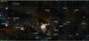 |
Fig. 1. Aladin DSS2 color image showing with white circles the positions of the clusters we survey here. The Galactic coordinates l and b are depicted by a green grid, and constellation limits for Carina, Vela, Centaurus, and Crux are plotted as yellow lines. |
3. Photometric observations
A first series of CCD UBVI photometry was carried out on 13 open clusters placed in the Galactic region that extends from 270° to 300° in Galactic longitude and from 7° to −5° in Galactic latitude. This region covers the Carina Arm, the interarm region between the Perseus and Carina arms, and also a part of the Local Arm. The observations were made on nine nights in April and May 2002, using the YALO (Yale, AURA, Lisbon, OSU)1 facilities at Cerro Tololo Inter-American Observatory (CTIO). The images were taken with a 2048 × 2048 px CCD attached to the 1.0 m telescope and the set of UBVI filters. The field of view is 10′×10′ given the 0.3″/px plate scale. All images were acquired using the ANDICAM2, which was moved to the 1.3 m CTIO telescope in 2003.
A second series of CCD photometry was implemented during March 2010 at CTIO to obtain UBVI photometry in two other clusters, NGC 4349 and Lynga 15; they lie at a slightly higher Galactic longitude (298°). Images in a first run were taken with the SMARTS 0.9 m telescope3 using a 2048 × 2046 px Tek2K detector4 with a scale 0.401″ px−1, covering thus 13.6′ on a side. A second run of images taken at the SMARTS 1.0 m telescope5 of the same clusters was carried out with a 4064 × 4064 px Y4KCam6 CCD with a scale of 0.289″ px−1, thus covering 20′×20′ on a side. The first run (at the 0.9 m) was not photometric, and therefore we tied all the images to the second run (at the 1.0 m), which was photometric. During this second run, we took multiple images of the standard star fields PG 1047 and SA98 (Landolt 1992).
Finally, in 2015, the open cluster vdBH 73, located at a lower longitude (∼273°), was observed in the UBVI filters with the 1.0 m Swope telescope7 at Las Campanas Observatory, Chile. On this occasion, direct images were acquired with the 4k × 4k E2V CCD with a scale of 0.435″ px−1, covering 29.7′×29.8′.
Short exposures were always obtained to avoid bright star saturation in the frame. Notwithstanding, very bright stars are sometimes lost. Details of air masses, seeing values, and exposure times per filter and telescope are listed in Table 2 for all the observations.
Log of observations at YALO (CTIO) and Las Campanas.
The basic reduction of the CCD science frames was made in the standard way using the IRAF 4 package ccdred. Photometry was performed using the IRAF DAOPHOT (Stetson 1987; Stetson et al. 1990) and photcal packages. Aperture photometry was performed to obtain the instrumental magnitudes of standard stars and some bright cluster stars. Profile-fitting photometry was performed in each program frame by constructing the corresponding point spread function. The zero-point of the instrumental magnitudes for each image was determined with aperture photometry and growth curves.
The transformation equations to convert instrumental magnitudes into the standard system were always of the form
 (1)
(1)
where u2, b2, v2, and i2 are the extinction coefficients computed for each night, and X is the air-mass. No color dependence of higher order was found for either filter.
In each case, detector coordinates were cross-matched with Gaia astrometry to convert pixels into equatorial α and δ for the equinox J2000.0, thus providing Gaia-based positions for the entire cluster catalog. This process was performed in three steps. First, the Astrometry.net8 service was used to assign (α, δ) coordinates to the brightest stars in our observed frames. The second step involved employing our own code, called astrometry9, to apply a transformation from pixel to equatorial coordinates to all the observed stars, using the coordinates already assigned to the brightest stars matched in the previous step. The algorithm in this code applies the affine transformation method developed by J. Elonen10 based on the work by Späth (2004). The transformation equations are of the form α = c0 + c1x + c2y, where α is the right ascension, (x, y) are the pixel coordinates, and the cX coefficients are fit (similarly for δ, more details on the code site). Finally, in the third step, we used another one of our open-source codes, called CatalogMatch11, to cross-match our frames (which by now had equatorial coordinates assigned) with Gaia DR212 data. The matching tolerance used here ranged from 2 to 4 arcsec, with mean minimum and maximum differences in the matches of 0.3 and 0.9 arcsec, respectively (for all the observed frames).
With the exception of cluster NGC 4349, the remaining objects in our sample have no dedicated photometric studies. We were still able to perform a comparison of our photometry in V, B, and (B − V) with available photometry from APASS DR10 (The AAVSO Photometric All-Sky Survey13), which has a magnitude limit near 18 mag (enough to identify the presence of red giant branch, RGB, stars), and Gaia DR2. In this comparison we placed particular emphasis on the clusters belonging to the observing runs in 2002 because they are mostly very faint.
For APASS data, we downloaded a region centered on each observed frame and cross-matched it with our data, taking care to remove bad matches by enforcing a tolerance of 0.7 arcsec on the matches for all the frames (this value was selected because it gave a reasonable number of matches with a minimum of bad-match contamination). We also compared our photometry with that from Gaia DR2 using the Carrasco photometric relationships14 between the Johnson-Cousins system and Gaia passbands. The process requires transforming the G magnitude into V and B magnitudes through the transformation equations provided there. For the V filter we employed the (G − V) versus (BP − RP) polynomial. For the B filter, no similar polynomial has been presented, therefore we fit our own using the same list of cross-matched Landolt standards as was used by Carrasco15. This third-degree polynomial is
![Mathematical equation: $$ \begin{aligned} {\begin{aligned} G - B = &0.003[0.009]-0.64[0.02]\,(BP-RP) \\&-0.42[0.03]\,(BP-RP)^2+0.067[0.007]\,(BP-RP)^3 \,, \end{aligned}} \end{aligned} $$](/articles/aa/full_html/2020/05/aa37141-19/aa37141-19-eq2.gif) (2)
(2)
where the values in brackets are the standard deviations of each coefficient, and the RMS of the residuals is σ ∼ 0.066. As a result of applying these two polynomials, we obtain transformed G magnitude values into VGaia and BGaia magnitudes, which we can use for a direct comparison with our own V and B magnitudes.
The results are shown in Table 3, where the ΔV, ΔB and Δ(B − V) columns display the mean differences between our photometry and APASS DR10 and Gaia DR2 data for all the observed regions. In each frame the groups of stars to compare were selected according to the filter criteria imposed by Carrasco: G < 13, σG < 0.01. The mean differences for V, B and (B − V) combining all the frames are shown in Fig. 2. Although there are no visible trends, there are offsets in the V and B magnitudes between our photometry and APASS of (ΔV = −0.07 ± 0.07, ΔB = 0.06 ± 0.08) and between our photometry and Gaia of (ΔV = −0.03 ± 0.04, ΔB = −0.01 ± 0.08). The reason for the differences found for the offsets between our data and APASS/Gaia is that APASS DR10 itself is offset from Gaia DR2 by (ΔV = 0.04 ± 0.07, ΔB = 0.05 ± 0.10), in the sense (Gaia – APASS). These values were found by directly cross-matching APASS data (for the regions where our 16 frames are located) with Gaia data, and applying the transformations for the G magnitude into V, B. In any case, these offsets are not relevant because we only use the (B − V) color in the analysis so that the offsets tend to compensate for each other and result in a lower value of ∼0.015 mag. The effect of this (B − V) offset in our photometry on the estimated photometric distances is addressed in Sect. 6.
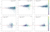 |
Fig. 2. Top row: differences between the APASS DR10 data for the V (left), B (center) magnitudes and (B − V) color (right) and our own photometry. Bottom row: same for Gaia DR2 data vs. our photometry. Details in the text. |
Mean differences between APASS and the Carrasco transformation polynomials and our own photometry.
Figure 3 shows the CCD V images of the clusters areas in which we carried out the photometric surveys. The series of panels shown from upper left to the lower right is ordered by increasing longitude and labeled with the cluster name inserted in every panel. Equatorial decimal coordinates, α and δ, for the J2000.0 equinox are shown in each panel as reference.
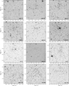 |
Fig. 3. V images (charts) of the observed clusters (names inserted) ordered from top to bottom and from left to right by increasing longitude. Decimal α and δ coordinates for the 2000 equinox are indicated. North and east are also shown. |
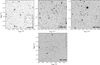 |
Fig. 3. continued. |
Final tables containing star number, x,y detector coordinates, and α, δ equatorial coordinates together with magnitude and colors are accessible in a separate form for each cluster at Vizier.
4. Photometric data analysis process: Gaia data and the ASteCA code
To analyze the large number of objects studied in this article in a systematic, reproducible, and homogeneous way, we used the ASteCA code16. The main goal of this code is to put the user apart as far as possible from the analysis of a stellar cluster to derive its fundamental parameters. We limit ourselves to a brief summary about the way the positional and photometric data are employed by the code. A complete description of the analysis carried out by ASteCA can be found in Perren et al. (2015) and Perren et al. (2017). The basic hypothesis of any stellar cluster analysis is that the region occupied by a real cluster and the surrounding field show a priori different properties. This means that we expect to see an increase in the stellar density (not always true) where a cluster is assumed to exist; the kinematic properties of cluster members are expected to differ from similar ones for the surrounding region; members of a cluster must be at a same distance, but nonmembers may show any distance; and the photometric diagrams composed of members of a cluster are expected to follow a well-defined stellar sequence, but field stars do not.
4.1. Gaia data
The second data release for the Gaia mission (Gaia Collaboration et al. 2018) was presented in April 2018 with improved coverage, particularly for the five-parameter astrometric solution. We crossed-match our complete set of photometric data with those of Gaia DR2 and employed the GaiaG magnitude, parallax, and proper motions in our analysis as described in Sect. 4.2.
No uncertainty-based cutoff was imposed on Gaia DR2 parallax or proper motion data following the advice given in Luri et al. (2018), who explained that even parallaxes with negative values or large uncertainties carry important information. Negative values in the parallax data were thus retained during the processing. The parallax values were processed with a Bayesian approach to obtain an independent estimate of the distance to each cluster. In this approach, the model for the cluster is taken from the accompanying tutorial by Bailer-Jones on inferring the distance to a cluster based on astrometry data17. The full model (i.e., the likelihood in the Bayesian approach) can be written as
![Mathematical equation: $$ \begin{aligned} \begin{aligned} P\left(\{\varpi \} | r_{\rm c}\right) =& \prod _{i=1}^{N} \int \int \frac{1}{2 \pi \sigma _{\varpi _{i}} s_{\rm c}} \\&\exp \left[-\frac{1}{2} \left( \frac{\left(\varpi _{i}-1 / r_{i}\right)^{2}}{ \sigma _{\varpi }^{2}} + \frac{\left(r_{i}-r_{\rm c}\right)^{2}}{s_{\rm c}^ {2}}\right)\right] \mathrm{d} r_{i}\,\mathrm{d} s_{\rm c} \end{aligned} ,\end{aligned} $$](/articles/aa/full_html/2020/05/aa37141-19/aa37141-19-eq3.gif) (3)
(3)
where {ϖ} is the set of all parallax values (our data), N is the number of processed stars in the cluster, ϖi and σϖi are the parallax value and its uncertainty for star i, ri is the distance to that star in parsec, sc is a shape parameter that describes the size of the cluster, and rc is the distance to the cluster (the parameter we wish to estimate). Our model marginalizes not only over the individual distances (ri; as done in the original model by Bailer-Jones), but also over the shape parameter (sc), estimating only the overall cluster distance rc using the parallax value and its uncertainty for each star in the decontaminated cluster region (the membership probabilities process is described with more detail in Sect. 4.2). The prior for the distance in the Bayesian model is a Gaussian centered at a maximum likelihood estimate of the distance to the cluster region, with a large standard deviation (1 kpc). This maximum likelihood was obtained through a differential evolution algorithm built into scipy18, applied in Eq. (3), that is, the model. The results of this analysis are shown in Sect. 5 and are discussed in Sect. 6.
We include in our analysis a two-sample Anderson-Darling test19, comparing the distribution of Gaia parallax and proper motions, between the cluster and the estimated stellar field regions, to quantify how similar these two regions are. The results of the test in each case are indicated with AD and the corresponding p-value20 in Fig. 7 and the similar figures for the remaining clusters. The p-value indicates the significance level at which the null hypothesis can be rejected: the lower the p-value, the higher the probability for the cluster region to be a true physical entity rather than a random clustering of field stars. When parallax and proper motions are used, three p-values are generated that are combined into a single p-value using Fisher’s combined probability test21.
4.2. The way ASteCA works
Since the first release of ASteCA, the code has grown considerably. The purpose of the tool and the core set of the analysis it is able to perform are still properly described in Perren et al. (2015), although several modifications have been implemented since. The most relevant changes include the ability to combine parallax and proper motion data in the membership analysis algorithm, which was initially purely photometric. This means that currently, up to seven dimensions of data can be used in this process: magnitude, three colors, parallax, and proper motions.
The several tasks performed by ASteCA can be roughly divided into three main independent analysis blocks: structural study including the determination of a cluster region identified primarily by an overdensity, individual membership probability estimation for stars inside the overdensity, and the search for the best-fit parameters.
The first block estimates center and radius values that in each case define the cluster region. Reliable estimates of these two quantities can only be achieved when a clear overdensity and a large number of members are detected. If a cluster is not clearly defined as an overdensity in the observed frame and if its boundaries are weakly established, ASteCA allows center and radius to be manually fixed because the automatic procedure may return incorrect values. We chose to fix all radius values manually because many of our observed frames are structurally sparse and with a low number of members, and display very noisy radial density profiles (RDP)22. Every point of the RDP was obtained by generating rings around the center defined for the potential cluster, that is, the comparison field. In our case, the comparison field may contain between one and ten regions with an area equal to that of the cluster, depending on the cluster area and the available size of the remaining frame. In each ring the number of stars (with no magnitude cut applied) is divided by the respective area to obtain a value of the radial density. To compute the density level of the field (foreground and background), outliers in the RDP are iteratively discarded to avoid biasing the final value. This procedure is repeated until it converges to an equilibrium value, equivalent to the density of the stellar field at a given distance from the potential cluster center.
King profile (King 1962) fittings were performed when a fit could be generated. No formal core or tidal radius are given because their values, due mainly to the shape of the RDP, were not within reasonable estimates (the process to fit the King profiles to the RDP returned either high and unrealistic values, or values with very large uncertainties). This might be due to the nonspheric geometry of sparse open clusters combined with the field contamination within the cluster region. Although photometric incompleteness is not taken into account in the generation of the RDP, these clusters are not strongly affected by crowding; thus we do not expect this to have a major effect on the estimated radii.
The second block assigns membership probabilities to the defined cluster region, an often disregarded process in simpler cluster studies, and removes the most probable field stars that contaminate this region. By itself, an overdensity does not guarantee the presence of a real cluster; an overdensity is frequently generated by random fluctuations in the field stellar density. To avoid this mistake, the properties for cluster and field stars must be compared. Ideally, we search for firm evidence of a cluster sequence at some evolutionary stage. ASteCA employs a Bayesian algorithm to compare the photometric, parallax, and proper motion distribution of the stars in the cluster region with a similar distribution in the surrounding field areas (Perren et al. 2015). Initially, the analysis was carried out in an N-dimensional data space that combined the G magnitude, parallax, and proper motions from Gaia with colors from our own photometry: (V − I), (B − V), (U − B). In this case, the data space where the algorithm works is therefore characterized by N = 7. Combining all the available data is not always optimal, however. A data dimension can sometimes introduce noise in the analysis instead of helping distinguish members from field stars. In our case, we found that using parallax and proper motions, that is, N = 3, resulted in more clearly defined cluster sequences than when we included photometric dimensions (with N = 7 as mentioned above).
Briefly, the algorithm compares the properties of this N-dimensional data space for stars inside (cluster region) and outside (field region) the adopted cluster limits. All the data dimensions are previously normalized (to prevent any dimension from outweighting others) and 4σ outliers are rejected. The position of every star inside the cluster in this data space is compared against each star in all the defined equivalent-area field regions, assuming a Gaussian probability density (centered at the given values for each data dimension, with standard deviations given by the respective uncertainties). This procedure is repeated hundreds or thousands of times (defined by the user), each time selecting different stars to construct an approximation of the clean cluster region. The result of this algorithm is thousands of probability values that are averaged to a final single membership probability value for each star within the cluster region.
This block ends with the cleaning of the photometric diagrams in the cluster region. The photometric diagram of each cluster region is divided into cells, and the same is done for the equivalent diagram of the field regions. The stellar density number found in the field is then subtracted from the cluster photometric diagram, cell by cell, starting with stars that have low membership probabilities. Therefore, the final cluster photometric diagrams contain not only star membership assignations, but are also cleaned from the expected field stellar contamination. This two-step process is of the utmost importance to ensure that the fundamental parameter analysis that follows is performed on the best possible approximation to the cluster sequence (particularly when the cluster contains only few members).
Finally, the third block estimates the cluster parameters by minimizing a likelihood function (Dolphin 2002) through employing a numerical optimization with a genetic algorithm (Charbonneau 1995). This last stage includes the assignment of uncertainties for each fitted parameter with a standard bootstrap method (Efron & Tibshirani 1986). Again, all of these processes are described in much more detail in Perren et al. (2015, 2017).
It is worth noting that unlike other tools (e.g., Yen et al. 2018), ASteCA does not fit isochrones to cluster sequences in photometric diagrams. Instead, it fits synthetic clusters generated from a set of theoretical isochrones, a given initial mass function, and completeness and uncertainties functions estimated directly from the observations. These synthetic clusters are represented as two- or three-dimensional CMDs, depending on the number of photometric colors available in our observations. The best-fit isochrones shown in green in the photometric diagrams in Fig. 6 for vdBH85 (and similar figures for the remaining clusters) are there for convenience purposes only, as a way to guide the eye.
The code makes use of the PARSEC v1.2S (Bressan et al. 2012) theoretical isochrones (obtained from the CMD service23), and the Kroupa (2002) form for the initial mass function. A dense grid of isochrones with fixed z and log(age) values is requested to the CMD service24, which are later used in the fundamental parameters estimation process. The full processing yields five parameters: metallicity, age, extinction, distance, and mass, along with their respective uncertainties. The binary fraction was always fixed to 0.3, a reasonable estimate for open clusters (Sollima et al. 2010). As for the final mass of each cluster, although the values are corrected by the effects of star loss due to photometric incompleteness at large magnitudes and the percentage of rejected stars with large photometric uncertainties, it is not corrected by the dynamical mass loss due to the cluster’s orbiting through the Galaxy. Hence, it should be regarded as a lower limit on the actual initial mass value.
From a practical point of view, the code proceeds as follows to estimate the cluster parameters: First, individual three-dimensional G vs. (B − V) vs. (U − B) photometric diagrams are analyzed, for which the metallicity is fixed to a solar value (z = 0.0152) in order to reduce the dimensionality of the parameter space, and thus its complexity. Although several of the diagrams described above in our case contain a rather small number of stars because of the U filter, they are very useful to obtain reddening and thus extinction by inspecting the (U − B) vs. (B − V) diagrams (e.g., Vázquez et al. 2008). The individual E(B − V) values in each region were always verified against the maximum values given in the Schlafly & Finkbeiner (2011) maps (hereafter S&F2011)25. The only information extracted from this first step, and in particular, by inspecting the (U − B) vs. (B − V) diagram, is thus a reasonable range for the E(B − V) parameter. Second, the analysis of the G versus (B − V) versus (V − I) diagram is carried out by restricting now the reddening space to the E(B − V) range obtained previously, while still fixing the metallicity to solar value. From this process we obtain estimates for the age, distance, and cluster mass. Finally, in a third stage, the parameter ranges derived above are applied, now including the metallicity as a free parameter. As a result of the entire procedure, we obtain a five-parameter best-fit model for each observed cluster, along with the associated one σ uncertainties for each one. In all the cases we adopted R = Av/E(B − V) = 3.1 to produce absorption-free distance moduli.
During the maximum likelihood and bootstrap processes, each observed cluster was compared to ∼2 × 10⁷ synthetic clusters. This number was obtained by combining the synthetic clusters that were generated in the maximum likelihood and bootstrap processes by varying the fundamental parameter values.
5. Cluster-by-cluster discussion of the structural and intrinsic parameters provided by ASteCA
We now present the results from the spatial and photometric analysis carried out with ASteCA, together with the outcome of the application of the Anderson-Darling test that compares parallax and proper motion distributions in cluster regions with their respective field regions. It is important to emphasize that the code always fits the best possible synthetic cluster to a given stellar distribution, regardless of whether it is a true open cluster or not.
Our sample contains clusters with a wide variety of properties: some are bright, clearly detached from the cluster background and therefore have a clearly defined main sequence (TR 13, TR 12, NGC 4349, vdBH 87, and vdBH 92). Others are faint, with a sparse star population and are easy to confuse with the background (vdBH 73, vdBH 85, vdBH 106, RUP 162, and RUP 85). Because we include very many figures in this paper, we therefore decided to add these sources to an appendix. We limit ourselves here to presenting the case of three extreme types of clusters according to the statement above: a poorly defined (vdBH 85) and a well-defined cluster (NGC 4349), and a source that is not a cluster (RUP 87).
5.1. van den Bergh-Hagen 85
The open cluster vdBH 85 appears in the sky slightly east of the center of the Vela constellation. The V chart in Fig. 3 shows a weak star concentration near the north side of the observed field that extends slightly to the southeast. The color-color and color-magnitude diagrams (from now on CCD and CMDs, respectively) of the entire field of view in Fig. 4 is just a dispersed stellar distribution that approximately ends in a compact accumulation at (B − V) = 1 and below G = 17 mag. Another clear feature is the structure at G = 16 mag in the two CMDs and for 1.2 < (B − V) < 1.7 mag, which resembles a red clump.
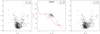 |
Fig. 4. From left to right: G vs. (V − I), (B − V) vs. (U − B), and V vs. (B − V) diagrams for all the stars observed in the region of van den Bergh-Hagen 85. The red dashed line in the CCD shows the position of the ZAMS (Aller et al. 1982). Insets in each diagram contain the number of stars in the cluster region (Nclust, black circles) and in the surrounding field (Nfield, gray circles). |
Figure 5 represents the spatial analysis carried out by ASteCA: results from the search for a stellar overdensity, the mean value for the stellar field density, the respective King profile attempting to fit the radial density profile, and the assumed radius. ASteCA detected an overdensity here that is difficult to see in Fig. 3. It stands out from the stellar background that is contained in a radius of 2.2 arcmin. It is characterized by a smooth RDP with nearly six times the background density at its peak, as shown in Fig. 5.
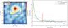 |
Fig. 5. From left to right, we present in the first panel a contour plot showing the position of the overdensity associated with vdBH 85. The green inner circle shows the cluster size, and the two black dashed-line squares enclose the region that ASteCA used to estimate the field stellar properties. The lower density values at the frame borders are an artifact of the kernel density estimate method that we employed to generate the density maps. Equatorial coordinates in decimal format are indicated. The color bar denotes the star number per square arcminute (linear scale). These values are slightly different from those in the panel to the right because they are obtained with a different method (nearest neighbors). The second panel shows the RDP as blue dots with standard deviations as vertical black lines. The King profile is shown as a dashed green line. The horizontal black line is the mean field stellar density. The vertical red line is the adopted cluster radius. |
In the following step, the removal of interlopers by comparison with the background field properties yields the field-decontaminated CCD (U − B) versus (B − V) and CMDs, G versus (B − V), and G versus (V − I). This removal was performed by comparing the stellar density in the photometric diagram of the cluster region (whose stars already have membership probabilities provided by ASteCA) with that of the surrounding field regions. These diagrams are shown in Fig. 6. We insert the results from the best synthetic cluster fitting to the field decontaminated diagrams in the middle panel of Fig. 6. In these three panels we also show the isochrone curves from which the best synthetic cluster fit was generated. These isochrones were generated using the maximum likelihood values found for the metallicity and age by averaging of theoretical isochrones taken from the employed grid. Again, this is just to guide the eye because ASteCA does not fit isochrones.
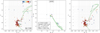 |
Fig. 6. From left to right: G vs. (V − I), (B − V) vs. (U − B), and G vs. (B − V) clean diagrams after field interlopers were removed by ASteCA over vdBH 85. The color of each star reflects its membership probability (MP). Corresponding values are in the color bar at the upper right corner in the G vs. (V − I) diagram (left) labeled MP. The CCD in the middle always shows fewer stars because of the U filter. The grid lines trace the edges of the three-dimensional photometric histograms we used to evaluate the likelihood function described in Sect. 4.2. The inset in the lower right corner in the G vs. (V − I) diagram shows the number of stars used by ASteCA to compare with synthetic clusters. The inset in the middle panel includes the final results for metallicity, log(age), E(B − V), the corrected distance modulus, and the total cluster mass provided by ASteCA. The green continuous line in the three diagrams is a reference isochrone. In particular, the green line in the CCD, middle panel, shows the most probable E(B − V) value fitting found by ASteCA. |
After the membership probabilities were established and field interlopers were removed, the two CMDs of all stars show a short but evident main sequence below G = 17 mag. Three magnitudes above the cluster turn-off, several stars appear at G = 14 mag. They might be part of the bright end of the giant branch. The comparison with the best fit of a synthetic cluster shows the following characteristics for vdBH 85:
-
(a)
The cluster is seen projected against a stellar field with moderate to low color excess. The best value corresponds to E(B − V) = 0.3, which agrees with the maximum value of 0.46 mag stated by S&F2011.
-
(b)
The free absorption distance modulus of vdBH 85 is 13.32 ± 0.12 mag, which implies a distance of 4.61 ± 0.26 kpc from the Sun. This by itself explains the extreme weakness of the cluster members.
Figure 7 includes three panels. The left panel shows the G mag versus Gaia parallax values (uncertainties indicated by horizontal bars) of cluster members, colored according to the estimated membership probabilities (color bar to the right). The Bayesian distance (dBayes) found by the code is shown here by a vertical blue dashed line, the equivalent ASteCA distance (dASteCA) with the green dotted line, the weighted average with the red dashed line (where the weights are the inverse of the parallax errors), and the naive estimate of obtaining the median of stars with parallax values greater than zero with the black dashed line. The middle panel shows the kernel density estimate of stars in the surrounding field region and the cluster region with black and red lines, respectively. For the Anderson-Darling test we used all the stars within the cluster region with Gaia data. In the right panel we summarize the distances in parsecs and errors, (dBayes) and dASteCA, followed by the corresponding parallax value, Plx, and corrected distance modulus, μ0. Both fittings are indicated by the vertical blue and green dashed lines. The final four text lines in the right panel list the AD values for Plx, PM(α), and PM(δ) from the Anderson-Darling test, followed by the corresponding p-values, and finally, the combined p-value.
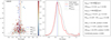 |
Fig. 7. Left panel: distribution of the parallax for all stars with membership probabilities in the cleaned cluster region as a function of the apparent magnitude G (the vertical color scale shows the membership probability of the star) in vdBH 85. Horizontal bars represent the parallax errors as given by Gaia. The different parallax value fittings are shown by dashed lines of different colors: blue shows the Bayesian parallax estimate, green the ASteCA photometric distance, red the weighted average, and black the median (without negative values). Middle panel: normalized comparison between the parallax distributions inside (red line) and outside the cluster region (dashed black line). The frame at the right summarizes the distances in parsecs according to the Bayesian analysis (dBayes) and ASteCA (dASteCA), followed by the corresponding parallax value, Plx, and corrected distance modulus (μ0). Both fittings are indicated by the vertical blue and green dashed lines. The last four text lines in the right panel list the AD values for Plx, PM(α), and PM(δ), followed by the corresponding p-values, and finally, the combined p-value. |
The distance estimated with parallax data from Gaia is almost 4 kpc larger than the distance obtained through the photometric analysis. This is most likely a failure of the Bayesian inference method we employed, and is caused by the large uncertainties associated with most of the probable cluster members. Further discussion is presented in Sect. 6. The Anderson-Darling test results in Fig. 7 suggest that the null hypothesis can be safely rejected given the combined p-value of 0.0. The Plx, PM(α), and PM(δ) results from the Anderson-Darling test leave no doubt that cluster region and surrounding comparison field come from quite different stellar populations.
We conclude that this object is a real and very old cluster, the oldest in our sample, approximately 7.50 ± 0.80 × 10⁹ yr old. This age places vdBH85 among the ten oldest clusters cataloged in the WEBDA26 and DAML27 (Dias et al. 2002) databases.
5.2. NGC 4349
This is an object in the Crux constellation, placed slightly south of its geometric center. At first glance, the V image in Fig. 3 shows a distinguishable star accumulation. The overall photometric CCD and CMDs in Fig. 8 show a prominent stellar sequence emerging at G ≈ 15 mag from the usual stellar structure produced by Galactic disk stars. The CCD highlights the reddened but compact sequence of blue stars placed immediately below the first knee of the intrinsic line. In addition, other bluer stars appear for (U − B) values lower than 0.0.
The ASteCA analysis revealed an extended overdensity of up to 70 stars per square arcminute. The density map of the observed frame shows two regions with very distinct mean stellar background densities. This is just an artifact generated by combining observations made with two different telescopes, as detailed in Sect. 3, and is the reason why the RDP shows such a strange shape, as seen in Fig. 9. We settled for a radius of ∼4 arcmin, which seems to contain most of the overdensity, and limited the analysis to the inner frame. The ASteCA estimation of memberships shows that inside the adopted cluster radius, the probable members of the cluster can easily be separated from the field region stars. This is shown in the respective CCD and CMDs in Fig. 10. The highest probabilities in the three diagrams show a somewhat narrow cluster sequence. In these cases (i.e., when a cluster sequence can be clearly defined down to the low-mass region), probable members can be identified by selecting a minimum probability value. We used P > 70%, which produces a reasonably clean sequence with an appropriate number of estimated members.
Comparison with synthetic clusters yielded that NGC 4349 is a cluster with the following properties:
-
(a)
A color excess of E(B − V) = 0.41 is found for the best-fitting synthetic cluster. Because the maximum color excess provided by S&F2011 in this location is 2.83, we conclude that most of the absorption is produced behind the position of NGC 4349.
-
(b)
The absorption-free distance modulus of NGC 4349 is 11.38 ± 0.11 mag, placing it at a distance of d = 1.88 ± 0.05 kpc from the Sun.
NGC 4349 is the only cluster in our sample with previous photographic photometry in the UBV system performed by Lohmann (1961). Because the differences between photographic and CCD photometry are typically large, we did not compare the data set of Lohmann with ours. According to Lohmann (1961), NGC 4349 is located at a distance of d = 1.7 kpc, almost 200 pc below our estimate. However, coincidences in terms of reddening, size, and background stellar density were found because Lohmann stated a cluster reddening of E(B − V) = 0.38 and similar cluster size. On the other hand, the Kharchenko Atlas28 (Kharchenko et al. 2005) gives a reddening value of E(B − V) = 0.38, which is similar to ours with a distance reported of d = 2.1 kpc, slightly above our estimate.
The distance found for this cluster using Gaia parallax data with no applied offset (processed with the Bayesian method described in Sect. 4.1) is 2.04 ± 0.03 kpc, just 160 pc larger than the photometric distance found by ASteCA. In Fig. 11 this distance was obtained by respecting the membership selection, thus ensuring that both analyses (the photometric analysis and this one) were performed over the exact same set of stars.
Parallax and proper motion distributions were tested using the Anderson-Darling statistics. With the exception of the comparison in the case of PM(δ) (where both samples, cluster and field, seem to come from the same distribution at a critical value just above 5%), the remaining two tests report quite different samples. Together with the photometric results, this confirms the true nature of NGC 4349.
High probability values for stars inside the overdensity and a clearly traced cluster sequence confirm the true nature of this object because the overdensity and the density profile are followed by a very well-defined and extended photometric counterpart. Because all these facts are self-consistent, we are confident that NGC 4349 is an open cluster that is 0.29 ± 0.09 × 10⁹ years old. The Kharchenko Atlas gives quite a similar value for the cluster age, reporting log(t) = 8.32 equivalent to 0.21 × 10⁹ yr.
5.3. Ruprecht 87
RUP 87 is located on the east side of the Vela constellation. According to Fig. 3, there is no relevant feature, but a rather poorly populated stellar field with a few bright stars that appear to be grouped toward the northern portion of the frame. The photometric diagrams in Fig. 12 show no appreciable stellar structure defining the presence of an open cluster. The few stars with (U − B) measures plotted in the respective CCD resemble that of a typical Galactic field dominated by a handful of late F- and G-type stars followed by a pronounced tail of red stars of presumably evolved types. Stars in the region 0 < (U − B) < 0.5 and 0 < (B − V) < 0.6 may be reddened early A- or/and late B-type stars.
Accordingly, after many trials, ASteCA was not able to detect an overdensity, as Fig. 13 clearly shows. This means that the potential locus occupied by the cluster RUP 87 is not unambiguously separated from the field background stars. Lacking a clear overdensity, we define the cluster region as that encircled by the green line, that is, the sector containing the apparently grouped bright stars. The RDP emerging from this analysis is quite noisy.
Comparing the density of the defined cluster region with that of the remaining stellar field, we find that the approximate number of probable members is 20 stars. When studying (purported) clusters with such a low estimated number of members, it is important to be extremely careful with the selection of stars that are considered to be members. If we were to simply select a small group of stars within a similar parallax range and analyzed their photometric diagram with ASteCA, we would probably obtain a somewhat reasonable fit because the code always finds the most likely solution, regardless of how dispersed the photometric diagram might be. If we a priori hand-pick a few stars with a common distance (parallax values), they are fit by a synthetic cluster with a very similar distance modulus as that defined by the selected parallax values, and some best-fit values for the remaining parameters. Similarly, the naive selection of stars with probabilities higher than 0.5 is not appropriate most of the times (unless a clear sequence can be defined, as in the case of NGC 4349) because this selection is biased toward brighter stars. This is because low-mass stars not only have larger associated uncertainties, they are also located in denser regions of the CMDs. This makes them much more likely to be assigned lower membership probabilities. A simple cut at 0.5 would generally result in a cluster sequence composed mostly of bright stars, without respecting the actual photometric density of the purported cluster (given by differences in photometric density of the cluster region versus field region). The stars that are selected within the cluster region should therefore be not only those with high membership probabilities or share a similar physical attribute (i.e., parallax). They should also be properly distributed in the photometric diagrams and as close as possible in number to the estimated number of members. As stated above, this is of particular importance for clusters with few members because the process of determining their best-fit parameters is driven by a handful of stars. This makes the analysis much more delicate.
In the case of RUP 87, we selected stars that had both high membership values and were similar in number to the estimated number of members for the cluster region. The 24 stars that remain in the adopted region along with the best fit are shown in Fig. 14. The code fits a somewhat old (3.1 × 10⁹ yr) synthetic cluster at a distance of ∼3900 pc.
Figure 15 shows that the distance estimated through Gaia parallaxes for the same set of stars is ∼6200 pc, which is more than 2000 pc away from the photometric estimate. This difference is too large to be consistent with a real cluster, even when possible offsets are taken into account. We determined whether this discrepancy might be solved as we did for vdBH 85 (see Sect. 6), we ran the same analysis with Bailer-Jones distances. The resulting weighted average for the distance is  pc. This distance is almost 800 pc larger than the photometric estimate, and 1500 pc smaller than the Gaia parallax estimate. Large differences like this are consistent with the fact that we did not analyze an actual cluster.
The Anderson-Darling test values for Plx and proper motions do not confirm clear differences between the cluster region and the stellar background in terms of kinematics and distance. The poverty of the photometric diagrams and the analysis of photometric distances versus parallax distances are all against the true existence of a cluster in the region RUP 87. In our interpretation, this is not a real entity, but the fluctuation of the star field.
6. Analysis of Gaia parallax distances
We complete our analysis by studying the distances yielded by ASteCA and those that can be obtained using parallaxes alone. Specifically, we cross-matched Plx data with our photometry, cluster by cluster, and processed them within a Bayesian framework (as explained in Sect. 4.1). The intention is to visualize the change in estimated distances when no correction is applied to the parallaxes and when current values taken from the literature are used.
In Fig. 16 we show the ASteCA versus Bayesian (parallax) distances with no offset applied (left), and the Bayesian parallax for each cluster (as the inverse of the distance) versus its difference with the ASteCA estimate (middle). It is evident from this figure that ASteCA distances are systematically smaller than those coming from the computation of parallax alone. The mean of the ASteCA minus parallax differences in distance is ∼ − 411 pc. The middle plot with the mean difference suggests that a correction of +0.028 mas needs to be applied to the Gaia DR2 parallax values. The cluster vdBH85 is omitted from Fig. 16 (left and middle plots) because the Bayesian framework applied on its parallax data yielded results that were clearly incorrect. This is shown in Fig. 7, where the estimated parallax distance exceeds 8 kpc compared with the photometric distance obtained by ASteCA of ∼4.6 kpc. Out of the ten clusters in our list of confirmed plus dubious clusters, vdBH85 is the oldest. This means that its main sequence is quite short and composed mostly of low-mass stars. More than 60% of its 146 estimated members have G > 18 mag, and almost 75% have Gaia DR2 parallax values with uncertainties larger than 0.1 mas (with a mean parallax uncertainty of ∼0.16 mas). Because of this, the Bayesian method fails to estimate a reasonable distance for this cluster, and we omit it from this analysis.
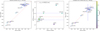 |
Fig. 16. Left: ASteCA (photometric) vs. Bayesian (parallax) distances for the clusters listed in Table 4 that are confirmed to be real clusters. No bias correction was applied to the parallax data. The color bar at the right indicates log(age) values. Center: offset (ASteCA – Bayes) for distances expressed as parallax in miliarcseconds. Right: same as left plot, with bias corrections from Lindegren et al. (+0.029 mas). The cluster vdBH85 is included here; its distance value is estimated from the list of individual distances reported by Bailer-Jones et al. (2018). |
A number of recent articles have found an offset in the Gaia parallax data that covers a range of approximately +0.05 mas. We selected three of these articles that fully cover this range to compare them with our results, which were obtained with no bias corrections: Lindegren et al. (2018), Schönrich et al. (2019), and Xu et al. (2019). Lindegren et al. processed the parallax of hundreds of thousands of quasars and derived a median difference with Gaia data of +0.029 mas. Schönrich et al. analyzed the radial velocity subset of Gaia DR2 with their own Bayesian inference tool and estimated a required +0.054 mas offset in the parallax data from Gaia DR2. Finally, Xu et al. used ∼100 stars with VLBI astrometry and found an offset of +0.075 mas with Gaia DR2 parallaxes. When we add the offsets given in Lindegren et al., Schönrich et al., and Xu et al. (+0.029, +0.054, +0.075 mas, respectively) to the parallax data, the agreement between ASteCA and the parallax distances improves at first and then rapidly worsens. The mean differences between photometric distances and parallax distances are ∼0.09 kpc, ∼0.39 kpc, and ∼0.62 kpc, using the Lindegren et al., Schönrich et al., and Xu et al. corrections, respectively.
We are unable to apply the Bayesian method described in Sect. 4.1 (as explained above) to vdBH85, therefore we considered the individual distance values obtained in Bailer-Jones et al. (2018). The authors used Bayesian inference to estimate distances (in parsec) to more than one billion stars using the Gaia DR2 parallax values by applying the correction reported by Lindegren et al.29. We cross-matched our list of members for vdBH85 and approximated the distance to the cluster as their average distance, weighted by the assigned uncertainties. Although this is a rather low-quality estimate because of the large uncertainties in the individual distances, as seen by the large error bars in Fig. 16 (right plot), it is still close to the photometric distance estimate. When we omit vdBH85 entirely, the Lindegren et al. mean difference improves to ∼0.05 kpc.
Our analysis thus indicates a required bias correction to Gaia parallaxes of +0.028 mas, which is very close to the value proposed by Lindegren et al.
In Sect. 3 we described that our (B − V) color has a small offset of ∼0.0153 mag when compared to the (transformed) Gaia photometry. ASteCA employs the extinction law by Cardelli et al. (1989, CCC law) with the O’Donnell (1994) correction for the near-UV, to transform E(B − V) values into absorptions for any filter. In our case, we used the GaiaG filter, whose absorption AG is related to E(B − V) as AG = c0 AV = c0 3.1 E(B − V), where c0 ≈ 0.829 according to the CCC law. The absorption  , that is, corrected for the offset in (B − V), can accordingly be written as
  . For the range of distance moduli in this work (∼11–14 mag), the effect of this correction on the distance in parsec extends from ∼30 to 100 pc. When we applied this (B − V) offset to our photometric distances and repeated the analysis, the +0.028 mas bias in Gaia parallaxes that we found initially was reduced to +0.023 mas. This is a lower value, but still very close to the bias reported by Lindegren et al.
An analysis of a more extended sample of clusters is certainly needed for conclusive results and to establish the detailed relation between distances from photometry and DR2 parallaxes. The results of the exercise presented in this section are included in the last four columns of Table 4.
Fundamental parameters and parallax distances obtained for the confirmed and probable clusters.
7. Discussion of results and concluding remarks
We have analyzed the fields of 16 cataloged open clusters located in a Galaxy sector covering approximately 270° to 300° in Galactic longitude, and mostly close to the formal Galactic plane at b = 0°. The cluster parameter estimates presented in this article are based on precise UBVI photometry analyzed in a automatic way by our code ASteCA. The code searches for a meaningful stellar overdensity and assigns membership probabilities by comparison with the surrounding stellar field. The next step establishes the physical properties of the best synthetic cluster that fits the distribution of cluster members in the CMDs and the CCD. Through this process, reddening, distance, age, mass, and metallicity are given. The most relevant inconvenience we have found with this cluster sample is that some of the clusters are extremely faint, which becomes evident in a visual inspection of their overall CCDs and CMDs. This becomes more difficult because the (U − B) index has mostly been available only for the bright and blue stars. This considerably reduced the data analysis space. Despite this, we were able to control the reddening solutions and obtained reliable distance estimates for the objects that were found to be true clusters by our code. In this way, we can safely reject RUP 87, vdBH91, RUP 88, Lynga 15, Loden 565, and NGC 4230, which most probably are random stellar fluctuations. The results for true and probable open clusters are shown in Table 4 in a self-explaining format.
When we average the metallicity for each cluster, shown in the second column of Table 4, the metal content is z = 0.0136 ± 0.006. The result agrees well with the assumption that the typical open cluster in the Milky Way has solar metallicity (z = 0.0152, Bressan et al. 2012).
Of the remaining ten objects, two are probable clusters with distances in the 4–5 kpc range. The cluster ages range from a few million years to almost 8 billion years in the case of vdBH 85. The vdBH 106 cluster is one of the oldest, but it is just a probableopen cluster, therefore its age needs be taken with caution. Two other objects, TR 13 and vdBH 92, are young, with ages close to and younger than 100 million years, respectively, and the remaining are all younger than 1 billion years.
A final remark concerns the spatial distribution of the eight real and two probable clusters listed in Table 4. These objects are plotted in Fig. 17 in the X − Y (upper) and X − Z (lower) planes of the Milky Way, following the usual sign convention. The Sun is placed at (0, 0). Superposed is the outline of the Carina Arm, taken from Vallée (2005). All these objects are plotted with open circles except, for the two youngest, which are shown with red squares. TR 13, one of the youngest (0.1 Gyr) and farthest (4.8 kpc) objects, is located at the external side of the Carina arm but appears well below the Galaxy plane at about −0.2 kpc. This means that it follows the warp of this arm, which has been mentioned among others by Cersosimo et al. (2009). The other young cluster, vdBH 92 (0.02 Gyr), is relatively far from the nucleus of the Carina Nebula in an intermediate zone between that region and the Sun, but is still seen close to the northwest side of the Carina Nebula at a distance that lies within the estimated maximum and minimum distance for Carina. vdBH 106 (3 Gyr) and vdBH 85 (7.5 Gyr) are the oldest objects in our search and are in turn placed well above the formal Galactic equator (0.3–0.4 kpc). TR 12 (0.7 Gyr) is another quite old object that is placed below the plane (−0.2 kpc) together with RUP 162 (1 Gyr). The remaining clusters are of middle age and lie relatively closely to the Galaxy plane.
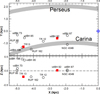 |
Fig. 17. X − Y (upper panel) and X − Z (lower plane) projection of the true and probable clusters in our sample (open circles). The red squares enclose the youngest clusters in our list (see Table 4). The thick gray lines in the upper panel show the trace of the Perseus and Carina arms according to Vallée (2005). The position of the Sun is shown by a blue crossed circle. The dashed line in the lower panel depicts the Galactic equator. |
We conclude for the photometric versus parallax distances that by adding ∼ + 0.028 mas to the computed cluster parallaxes from Gaia DR2, the level of agreement with the photometric distances improves considerably. When the small offset found for the (B − V) color is taken into account, this value drops to +0.023 mas, which is only 0.006 mas lower than the correction applied by Lindegren et al., +0.029 mas. This supports the evidence that indicated this offset over higher values proposed in the literature. Our cluster sample is not large enough to permit drawing stronger conclusions on this matter, particularly regarding the possible dependence of the correction on distance.
This list was kindly provided by Carrasco upon our request. We thank Dr Carrasco very much for sharing this data.
The null hypothesis (H0) is the hypothesis that the distributions of the two samples are drawn from the same population. The significance level (α) is the probability of mistakenly rejecting the null hypothesis when it is true, also known as Type I error. The p-value indicates the α with which we can reject H0. The usual 5% significance level corresponds to an AD test value of 1.961 for the case of two samples.
The radius values are estimated using the frames in pixel coordinates, and then converted into arcminutes.
Grid values: z range [0.0005, 0.0295] with a step of 0.0005; log(age) range [7, 9.985] with a step of 0.015
Through the NASA/IPAC service https://irsa.ipac.caltech.edu/applications/DUST/
This is not to be confused with the Bayesian inference method described in Sect. 4.1. These are two very different processes.
Acknowledgments
G.P., E.E.G., M.S.P. and R.A.V. acknowledge the financial support from CONICET (PIP317) and the UNLP. AM acknowledges the support from the Portuguese Strategic Programme UID/FIS/00099/2019 for CENTRA. The authors are very much indebted with the anonymous referee for the helpful comments and suggestions that contributed to greatly improving the manuscript. This research was made possible through the use of the AAVSO Photometric All-Sky Survey (APASS), funded by the Robert Martin Ayers Sciences Fund and NSF AST-1412587. This research has made use of the WEBDA database, operated at the Department of Theoretical Physics and Astrophysics of the Masaryk University. This research has made use of the VizieR catalog access tool, operated at CDS, Strasbourg, France (Ochsenbein et al. 2000). This research has made use of “Aladin sky atlas” developed at CDS, Strasbourg Observatory, France (Bonnarel et al. 2000; Boch & Fernique 2014). This research has made use of NASA’s Astrophysics Data System. This research made use of the Python language v3.7.3 (van Rossum 1995) and the following packages: NumPy (http://www.numpy.org/) (Van Der Walt et al. 2011); SciPy (http://www.scipy.org/) (Jones et al. 2001); Astropy (http://www.astropy.org/), a community-developed core Python package for Astronomy (Astropy Collaboration 2013); matplotlib (http://matplotlib.org/) (Hunter 2007); emcee (http://emcee.readthedocs.io) (Foreman-Mackey et al. 2013); corner.py (https://corner.readthedocs.io) (Foreman-Mackey 2016).
References
- Aller, L. H., Appenzeller, I., Baschek, B., et al. 1982, Landolt-Börnstein: Numerical Data and Functional Relationshipsin Science and Technology– New Series, Gruppe/Group 6 Astronomy and Astrophysics, Volume 2 Schaifers/Voigt:Astronomy and Astrophysics/Astronomie und Astrophysik, Stars andStar Clusters/Sterne und Sternhaufen [Google Scholar]
- Astropy Collaboration (Robitaille, T. P., et al.) 2013, A&A, 558, A33 [NASA ADS] [CrossRef] [EDP Sciences] [Google Scholar]
- Avedisova, V. S. 2002, Astron. Rep., 46, 193 [NASA ADS] [CrossRef] [Google Scholar]
- Bailer-Jones, C. A. L., Rybizki, J., Fouesneau, M., Mantelet, G., & Andrae, R. 2018, AJ, 156, 58 [NASA ADS] [CrossRef] [Google Scholar]
- Boch, T., & Fernique, P. 2014, in Astronomical Data Analysis Software and Systems XXIII, eds. N. Manset, & P. Forshay, ASP Conf. Ser., 485, 277 [NASA ADS] [Google Scholar]
- Bonnarel, F., Fernique, P., Bienaymé, O., et al. 2000, A&AS, 143, 33 [NASA ADS] [CrossRef] [EDP Sciences] [Google Scholar]
- Bossini, D., Vallenari, A., Bragaglia, A., et al. 2019, A&A, 623, A108 [NASA ADS] [CrossRef] [EDP Sciences] [Google Scholar]
- Bressan, A., Marigo, P., Girardi, L., et al. 2012, MNRAS, 427, 127 [NASA ADS] [CrossRef] [Google Scholar]
- Cantat-Gaudin, T., Jordi, C., Vallenari, A., et al. 2018, A&A, 618, A93 [NASA ADS] [CrossRef] [EDP Sciences] [Google Scholar]
- Cardelli, J. A., Clayton, G. C., & Mathis, J. S. 1989, ApJ, 345, 245 [NASA ADS] [CrossRef] [Google Scholar]
- Carraro, G., Vázquez, R. A., Moitinho, A., & Baume, G. 2005, ApJ, 630, L153 [NASA ADS] [CrossRef] [Google Scholar]
- Carraro, G., Costa, E., & Ahumada, J. A. 2010, AJ, 140, 954 [NASA ADS] [CrossRef] [Google Scholar]
- Cersosimo, J. C., Mader, S., Figueroa, N. S., et al. 2009, ApJ, 699, 469 [NASA ADS] [CrossRef] [Google Scholar]
- Charbonneau, P. 1995, ApJS, 101, 309 [NASA ADS] [CrossRef] [Google Scholar]
- Dias, W. S., Alessi, B. S., Moitinho, A., & Lépine, J. R. D. 2002, A&A, 389, 871 [NASA ADS] [CrossRef] [EDP Sciences] [Google Scholar]
- Dolphin, A. E. 2002, MNRAS, 332, 91 [NASA ADS] [CrossRef] [Google Scholar]
- Efron, B., & Tibshirani, R. 1986, Stat. Sci., 1, 54 [NASA ADS] [CrossRef] [Google Scholar]
- Foreman-Mackey, D. 2016, J. Open Sour. Soft., 1, 24 [NASA ADS] [CrossRef] [Google Scholar]
- Foreman-Mackey, D., Hogg, D. W., Lang, D., & Goodman, J. 2013, PASP, 125, 306 [CrossRef] [Google Scholar]
- Gaia Collaboration (Brown, A. G. A., et al.) 2018, A&A, 616, A1 [NASA ADS] [CrossRef] [EDP Sciences] [Google Scholar]
- Hunter, J. D., et al. 2007, Comput. Sci. Eng., 9, 90 [NASA ADS] [CrossRef] [Google Scholar]
- Janes, K., & Adler, D. 1982, ApJS, 49, 425 [NASA ADS] [CrossRef] [Google Scholar]
- Jones, E., Oliphant, T., Peterson, P., et al. 2001, SciPy: Open source scientific tools for Python [Online; Accessed 2016–06-21] [Google Scholar]
- Kharchenko, N. V., Piskunov, A. E., Röser, S., Schilbach, E., & Scholz, R.-D. 2005, A&A, 438, 1163 [NASA ADS] [CrossRef] [EDP Sciences] [MathSciNet] [Google Scholar]
- King, I. 1962, AJ, 67, 471 [NASA ADS] [CrossRef] [Google Scholar]
- Kroupa, P. 2002, Science, 295, 82 [NASA ADS] [CrossRef] [PubMed] [Google Scholar]
- Landolt, A. U. 1992, AJ, 104, 340 [NASA ADS] [CrossRef] [Google Scholar]
- Lindegren, L., Hernández, J., Bombrun, A., et al. 2018, A&A, 616, A2 [NASA ADS] [CrossRef] [EDP Sciences] [Google Scholar]
- Lohmann, W. 1961, Astron. Nachr., 286, 105 [NASA ADS] [CrossRef] [Google Scholar]
- Luri, X., Brown, A. G. A., Sarro, L. M., et al. 2018, A&A, 616, A9 [NASA ADS] [CrossRef] [EDP Sciences] [Google Scholar]
- Magrini, L., Stanghellini, L., Corbelli, E., Galli, D., & Villaver, E. 2009, VizieR Online Data Catalog: J/A+A/512/A63 [Google Scholar]
- Moitinho, A. 2010, in Star Clusters: Basic Galactic Building Blocks Throughout Time and Space, eds. R. de Grijs, & J. R. D. Lépine, IAU Symp., 266, 106 [NASA ADS] [Google Scholar]
- Moitinho, A., Vázquez, R. A., Carraro, G., et al. 2006, MNRAS, 368, L77 [NASA ADS] [CrossRef] [Google Scholar]
- Monteiro, H., & Dias, W. S. 2019, MNRAS, 487, 2385 [NASA ADS] [CrossRef] [Google Scholar]
- Ochsenbein, F., Bauer, P., & Marcout, J. 2000, A&AS, 143, 23 [NASA ADS] [CrossRef] [EDP Sciences] [Google Scholar]
- O’Donnell, J. E. 1994, ApJ, 422, 158 [NASA ADS] [CrossRef] [Google Scholar]
- Perren, G. I., Vázquez, R. A., & Piatti, A. E. 2015, A&A, 576, A6 [NASA ADS] [CrossRef] [EDP Sciences] [Google Scholar]
- Perren, G. I., Piatti, A. E., & Vázquez, R. A. 2017, A&A, 602, A89 [NASA ADS] [CrossRef] [EDP Sciences] [Google Scholar]
- Ruprecht, J., Balazs, B., & White, R. E. 1996, VizieR Online Data Catalog: VII/101A [Google Scholar]
- Schlafly, E. F., & Finkbeiner, D. P. 2011, ApJ, 737, 103 [NASA ADS] [CrossRef] [Google Scholar]
- Schönrich, R., McMillan, P., & Eyer, L. 2019, MNRAS, 487, 3568 [NASA ADS] [CrossRef] [Google Scholar]
- Sollima, A., Carballo-Bello, J. A., Beccari, G., et al. 2010, MNRAS, 401, 577 [NASA ADS] [CrossRef] [Google Scholar]
- Soubiran, C., Cantat-Gaudin, T., Romero-Gómez, M., et al. 2018, A&A, 619, A155 [NASA ADS] [CrossRef] [EDP Sciences] [Google Scholar]
- Späth, H. 2004, Math. Commun., 9, 27 [NASA ADS] [Google Scholar]
- Stetson, P. B. 1987, PASP, 99, 191 [NASA ADS] [CrossRef] [Google Scholar]
- Stetson, P. B., Davis, L. E., & Crabtree, D. R. 1990, CCDs in astronomy, ed. G. H. Jacoby, ASP Conf. Ser., 8, 289 [NASA ADS] [Google Scholar]
- Tadross, A. L. 2011, J. Kor. Astron. Soc., 44, 1 [NASA ADS] [CrossRef] [Google Scholar]
- Trumpler, R. J. 1930, Lick Obs. Bull., 420, 154 [NASA ADS] [CrossRef] [Google Scholar]
- Vallée, J. P. 2005, AJ, 130, 569 [NASA ADS] [CrossRef] [Google Scholar]
- van den Bergh, S., & Hagen, G. L. 1975, AJ, 80, 11 [NASA ADS] [CrossRef] [Google Scholar]
- Van Der Walt, S., Colbert, S. C., & Varoquaux, G. 2011, Comput. Sci. Eng., 13, 22 [CrossRef] [Google Scholar]
- van Rossum, G. 1995, Python tutorial, Report CS-R9526, pub-CWI, pub-CWI:adr [Google Scholar]
- Vázquez, R. A., May, J., Carraro, G., et al. 2008, ApJ, 672, 930 [NASA ADS] [CrossRef] [Google Scholar]
- Xu, S., Zhang, B., Reid, M. J., Zheng, X., & Wang, G. 2019, ApJ, 875, 114 [NASA ADS] [CrossRef] [Google Scholar]
- Yen, S. X., Reffert, S., Schilbach, E., et al. 2018, A&A, 615, A12 [NASA ADS] [CrossRef] [EDP Sciences] [Google Scholar]
Appendix A: Cluster-by-cluster discussion of the structural and intrinsic parameters provided by ASteCA
The 13 clusters in this appendix are ordered according to their longitude, as shown in Table 1. The remaining 3 analyzed clusters were presented in Sect. 5.
A.1. van den Bergh-Hagen 73
The cluster vdBH 73 is placed in almost the center of the Vela constellation well at the northeast border of the Carina constellation. The visual chart of the region in Fig. 3 shows a small and compact grouping of stars at the very center of the frame, surrounded by a dense stellar field. The inspection of the CCD and CMDs for all the stars observed in the targeted region in Fig. A.1 gives no clear indications about a cluster there, likely because of the field stellar contamination. A few stars in the CMDs of Fig. A.1 are above G = 15 mag, and at higher magnitudes, the CMDs strongly widen. The reddening in the CCD in the right panel in Fig. A.1 is quite strong and displaces the bulk of stars entirely toward the red side. A few blue stars with negative (U − B) values appear to be strongly affected by variable reddening.
The left panel in Fig. A.2 shows a pronounced stellar overdensity of 2.2 arcmin radius, coincident with the location expected for vdBH 73. This overdensity appears to be immersed in a region of large field stellar contamination. As shown in the RDP to the right, the density peak is about four times above the mean for the field.
The CMDs in Fig. A.3, left and right panels, show a cluster main sequence subtending 1.5 magnitudes and a faint giant branch with stars up to G = 15 mag. The (B − V) versus (V − I) CCD is shown in the middle panel instead of the (B − V) versus (U − B) diagram because the latter did not contain enough stars to be of use in the extinction estimation process. Although the CMDs after the removal of interlopers look somewhat noisy, stars with membership probabilities above ∼0.7 clearly trace the sequence of an evolved cluster. The best-fit of a synthetic cluster yields the following results:
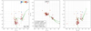 |
Fig. A.3. Same as Fig. 6 for vdBH 73 with the (B − V) vs. (V − I) diagram instead of the (B − V) vs. (U − B) diagram. |
-
(a)
The cluster is immersed in a region of moderate absorption because the mean of the reddening is E(B − V) = 1.06, which is compatible with those provided by S&F2011, who found a maximum E(B − V) of about 1.2 mag toward vdBH 73.
-
(b)
The absorption-free distance modulus is 13.50 ± 0.26 mag, placing this object at 5.01 ± 0.61 kpc from the Sun.
From the photometric point of view, the existence of a well-outlined cluster main sequence and the high probability memberships of the stars confirm the real entity of vdBH 73. The usage of parallax data from Gaia shows a good agreement in distance, reaching up 5.48 ± 0.44 kpc in the sense that Gaia parallaxes place the cluster farther than photometry does. This difference improves when an offset is applied to the parallax data, as shown in Sect. 7. The Anderson-Darling test applied to parallax and proper motion data demonstrates that the null hypothesis can indeed be rejected with a combined p-value of 0.0. This means that a real cluster is present in this region.
We conclude from our analysis that van den Bergh-Hagen 73 is an intermediate-age cluster that is about 0.78 ± 0.09 × 10⁹ years old.
A.2. Ruprecht 85
Ruprecht 85 belongs to the south side of the Vela constellation close to the border of the Carina region. This cluster appears in Fig. 3 as a slight increment in the stellar field toward the north part in the respective frame. The overall stellar photometric diagrams as shown in Fig. A.5 do not show any cluster sequence, but a vertical strip of stars emerging from a poorly populated stellar field above G = 14 mag defined by disk stars.
The structural analysis performed by ASteCA yields a clean overdensity at the location of this object that appears to subtend an almost circular area with a radius between 2–3 arcmin; see the left panel of Fig. A.6. As shown in the right panel of Fig. A.6, the RDP is well developed and with a stellar density five times above the background level. The photometric diagrams, CCD and CMDs of stars with membership probabilities above 0.48 and up to 1.0 shown in Fig. A.7 depict a rather noisy main sequence sweeping 3.5 mag. Combining structural evidences with evidences coming from the photometric diagrams we conclude that RUP 85 is a real entity. As for the cluster parameters of the best synthetic cluster fitting the observations it is found that:
-
(a)
As is the case with vdBH 73, RUP 85 is also placed in a region of moderate color excess. The cluster has E(B − V) = 1.06, also entirely in line with a maximum E(B − V) of 2 mag according to S&F2011.
-
(b)
The free absorption distance modulus is 13.40 ± 0.12 mag, corresponding to a distance d = 4.80 ± 0.26 kpc.
The results from the Anderson-Darling test in Fig. A.8 applied to Plx, PM(α), and PM(δ) clearly indicate that the cluster region and the surrounding background population come from quite different stellar populations. Therefore the null hypothesis can be rejected.
We conclude that RUP 85 is a real open cluster that is about 0.18 ± 0.03 × 10⁹ years old.
A.3. van den Bergh-Hagen 87
Like RUP 85, vdBH 87 is seen toward the south of the Vela constellation close to the border with Carina. A weak grouping of stars placed toward the north of the frame is shown in Fig. 3. In turn, the CMDs in Fig. A.9 seem to reflect a typical stellar disk sequence up to approximately G = 15 mag, with an amorphous distribution at the bright end. The CCD, on the other hand, is rather poor.
A stellar overdensity reaching about seven times the field stellar density is shown in Fig. A.10. The spatial structure of this overdensity suggests an elongation in right ascension and an RDP characterized by a very narrow density peak followed by a stellar coronal distribution at about 1.5 arcmin from the center. The clean CMDs in Fig. A.11 clearly show the nature of vdBH 87 because inside this overdensity, a clear and narrow cluster main sequence is evident. Its sequence extends for more than 5 mag in the CMDs, including stars with very low membership probabilities well detached from the sequence, in the range from 0.0 to 0.98. The parameters of the synthetic cluster that best fits the real stellar distributions are listed below.
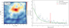 |
Fig. A.10. Same as Fig. 5 for vdBH 87. |
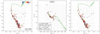 |
Fig. A.11. Same as Fig. 6 for vdBH 87. |
-
(a)
The color excess is E(B − V) = 0.56, indicating thus a moderate absorption in the cluster direction. This color excess value in turn is below the maximum reddening E(B − V) = 2.9 computed in the region by S&F2011.
-
(b)
The corrected distance modulus is 11.59 ± 0.09 mag, implying a distance of d = 2.08 ± 0.09 kpc. The cluster is not far from the Sun, and this closeness explains the moderate color excess we found.
The results of applying the Anderson-Darling test in Fig. A.12 are coincident with what ASteCA found: cluster and field regions are quite different not only from the photometric perspective, but also from a kinematic view. In conclusion, vdBH 87 is a real open cluster that is 0.25 ± 0.08 × 10⁹ years old.
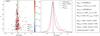 |
Fig. A.12. Same as Fig. 7 for vdBH 87. |
A.4. van den Bergh-Hagen 92
Placed south of Vela, near the eastern border with Carina, vdBH 92 is a relevant handful of bright stars as shown in the V image of Fig. 3. The CMDs and CCD for all stars in the region, as shown in Fig. A.13, depict a narrow stellar sequence with some scatter at their respective bright ends. Particularly the CCD shows a group of F- and G-type stars close to the intrinsic line, and another group of stars below the intrinsic line that might be B- and A-type stars displaced by the reddening effect.
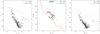 |
Fig. A.13. Same as Fig. 4 for vdBH 92. |
The ASteCA analysis in Fig. A.14 revealed a well-isolated stellar overdensity that rose above the field stellar density of about six stars per square arcminute. We identify this overdensity with vdBH 92. Notwithstanding the noisy RDP, the limits of the overdensity can still be well established. As indicated in Fig. A.15, only a few stars have been found inside the cluster limits, mostly with high membership values. Despite the low number of members, a cluster main sequence extended by seven magnitudes is visible. The comparison with synthetic clusters made by ASteCA yields that
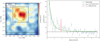 |
Fig. A.14. Same as Fig. 5 for vdBH 92. |
-
(a)
the best-fit of a synthetic cluster to the clean data in Fig. A.15 indicates a color excess of E(B − V) = 0.65. Because the maximum color excess provided by S&F2011 is 2.34 for this zone, we conclude that most of the absorption is produced behind the position of vdBH 92. This object is therefore placed in front of a strong absorption region.
-
(b)
the absorption-free distance modulus becomes 12.07 ± 0.09 mag, which places vdBH 92 at a distance of d = 2.59 ± 0.11 kpc.
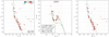 |
Fig. A.15. Same as Fig. 6 for vdBH 92. |
By applying the Anderson-Darling test, we note that the parallax distributions for stars inside and outside the cluster boundaries are not sufficiently different from each other to reach the 5% critical value, as indicated in the right panel of Fig. A.16. However, proper motions are quite different in both regions. We combine this last finding with the well-defined overdensity, which in turn shows a reasonable and extended cluster main sequence, and conclude that the two samples come from different populations.
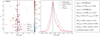 |
Fig. A.16. Same as Fig. 7 for vdBH 92. |
These results together confirm the true nature of vdBH 92. This young cluster is 0.02 ± 0.01 × 10⁹ years old; it is the youngest true cluster in our sample.
A.5. Trumpler 12
This object is placed on the west side of the Carina HII region, where it appears as a sparse handful of bright stars in Fig. 3. The CMDs in Fig. A.17, including all stars in the region, show the following patterns: there is a wide grouping of stars below G = 18 mag, but to the right side of it, and at this magnitude value, a narrow structure of stars up to G = 14 mag is also slightly displaced to the blue side. From G = 18 mag, a typical vertical galactic disk population rises as well.
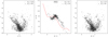 |
Fig. A.17. Same as Fig. 4 for TR 12. |
ASteCA detected a main overdensity in a region of high stellar contamination, as shown in Fig. A.18. This overdensity is characterized by a quite noisy RDP, which is partly explained by the background density: at the peak of the RDP, this is less than twice as high. Under this condition, it is difficult to fix an appropriate radius for the overdensity. We tentatively adopt a radius of ∼2 arcmin as a reasonable compromise. The membership probabilities in the zone of the overdensity are mostly above 0.5, as indicated in Fig. A.19. Again, as in vdBH 87, the handful of stars with a low membership probability are very well detached from the main cluster sequence. A clear cluster main sequence is shown in Fig. A.19 to span about 4–5 mag. These stars belong to the tiny blue and narrow sequence that is easily detected in the diagrams of Fig. A.17 between G = 12 and G = 16 mag. Comparison with synthetic clusters yields the following values:
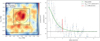 |
Fig. A.18. Same as Fig. 5 for TR 12. |
-
(a)
A color excess of E(B − V) = 0.31 is found for the best fit. Based on the maximum color excess provided by S&F2011 of 0.50, we find that TR12 is placed in a zone of low absorption.
-
(b)
The absorption-free distance modulus is 12.7 ± 0.09 mag, representing a distance of 3.50 ± 0.15 kpc. At this distance and with low absorption, it is reasonable to find a high stellar background density, as shown in Fig. A.18.
Based on the Anderson-Darling statistics shown in Fig. A.19, the proper motions for the cluster and for the field population belong to different samples. On the other hand, the parallaxes cannot be safely separated into distinct stellar regions.
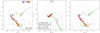 |
Fig. A.19. Same as Fig. 6 for TR 12. |
 |
Fig. A.20. Same as Fig. 7 for TR 12. |
The clear cluster sequence and the low p-value (0.003) obtained with the AD test lead us to conclude that TR 12 is a real cluster and is about 0.70 ± 0.10 × 10⁹ years old.
A.6. van den Bergh-Hagen 91
vdBH 91 is a potential cluster at the west side of Carina HII region, specifically, near the northern border of this constellation with Vela. No relevant stellar structure appears in the V image of Fig. 3, but a common pattern of a Galactic field star near the Galactic plane. The overall CMDs in Fig. A.21 show a stellar sequence that at first sight, resembles the usual diagrams for open clusters. In turn, the CCD is dominated by a tail of F- and G-type stars prolonged by red stars. We also note some reddened early-type stars for negative (U − B) indices.
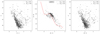 |
Fig. A.21. Same as Fig. 4 for vdBH 91. |
ASteCA found two well-separated stellar overdensity peaks in Fig. A.22, whose relevance in terms of structure is not important given the overall low stellar density of the field. The noisy RDP by itself proves the poverty of the entire field we surveyed in terms of star numbers. After some attempts to search for a cluster sequence, we asked ASteCA to estimate the probabilities for stars inside an adopted radius of ∼2.5 arcmin, shown in Fig. A.22 (right). As shown in Fig. A.23, almost 100 stars inside the circle associated with vdBH 91 were found in the CMDs. No clear cluster sequence is traced by stars with high probabilities, which are scattered across the entire CMD. The absence of a cluster sequence combined with the poor and noisy overdensity all argue against the reliability of this cluster.
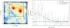 |
Fig. A.22. Same as Fig. 5 for vdBH 91. |
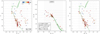 |
Fig. A.23. Same as Fig. 6 for vdBH 91. |
The Anderson-Darling test in the right panel of Fig. A.24, is clear regarding the true nature of vdBH 91 because the high combined p-value indicates that the null hypothesis (cluster and field areas come from the same originating distribution) cannot be reasonably rejected. This result disgrees with the results reported by Kharchenko et al. (2005), who found that vdBH 91 is a cluster at 0.75 kpc, approximately 0.16 × 10⁹ yr old, and affected by a mean color excess E(B − V) = 0.08.
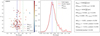 |
Fig. A.24. Same as Fig. 7 for vdBH 91. |
We conclude that vdBH 91 is a random fluctuation of the stellar foreground and background, and not a real entity.
A.7. Trumpler 13
TR 13 is a weak object also at the southwest of the Carina HII region, seen as a diffuse but extended stellar accumulation near the center of the V image in Fig. 3. The two CMDs in Fig. A.25 show an uncommon pattern: above G = 17.5 mag, the stellar sequence splits into two branches, one of which extends to the bluest side, while the other branch follows the common representation of galaxy disk stars. The situation is the same in the CCD: a wide and reddened band of potential B-type stars is placed at (B − V) < 0.45 and −0.25 < (U − B) < 0.5, with a few more stars at the negative (U − B) index, while another strip of stars extends from the characteristic place for F-type stars and reaches the red tail, including probable giant stars.
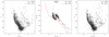 |
Fig. A.25. Same as Fig. 4 for TR 13. |
Figure A.26 indicates that ASteCA found a spatially extended overdensity mostly elongated north-south, which is nearly four times above a mean field stellar density of ∼26 stars per square arcminutes at its peak. Based on the shape and extension of the overdensity, we adopted a formal radius of ∼2.5 arcmin and asked ASteCA to compute the membership probabilities for the stars inside the area. Figure A.27 shows that after field interlopers are removed, almost 170 stars are left composing a narrow cluster main sequence that extends for more than five magnitudes. Consequently, when we compare this with synthetic clusters, the results yield
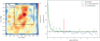 |
Fig. A.26. Same as Fig. 5 for TR 13. |
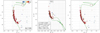 |
Fig. A.27. Same as Fig. 6 for TR 13. |
-
(a)
a color excess of E(B − V) = 0.56 for the best fit of a synthetic cluster. Because the maximum color excess provided by S&F2011 is 1.94, it is reasonable to conclude that most of the absorption is produced behind the position of TR 13.
-
(b)
that the absorption-free distance modulus of TR 13 is estimated to be 13.41 ± 0.15 mag, placing it at a distance of 4.81 ± 0.33 kpc from the Sun.
The Anderson-Darling statistics in the right panel of Fig. A.28 confirms the photometric results: cluster area and the surrounding field region possess quite different properties.
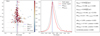 |
Fig. A.28. Same as Fig. 7 for TR 13. |
The selected probable members inside the overdensity confirm the true nature of this object because the over density and the density profile are followed by a very well defined and extended photometric counterpart. All these facts combined with the results from the Anderson-Darling test are self-consistent, so that we are confident that TR 13 is a young cluster of 0.11 ± 0.02 × 10⁹ years.
A.8. van den Bergh-Hagen 106
This cluster is placed at the southeast of the Vela constellation. The stellar field where it is placed is not very dense and has no relevant features, except for a few moderately bright stars, as shown in Fig. 3. The CMDs shown in Fig. A.29 represent typical photometric features: structures of Galactic fields with no cluster inside. The CCD in the same figure shows a reduced number of stars below the intrinsic line (probably reddened late B- and A-types) and a tail of stars from of late F-types to M-type stars, some of them probably giants, at the red end. The ASteCA spatial analysis found some stellar clumps, as shown in the left panel of Fig. A.30. We focus on the main clump at the very center of the frame because here we see the highest overdensity peak with about three times more stars than at the mean stellar background density of about 11 stars per square arcmin. We assume that most of stars in vdBH 106 must be included there, so that the cluster parameters are expected to be well established. The RDP to the right appears poorly defined because it reflects the irregular and low stellar density even inside the zone we selected to investigate the cluster parameters. Only 82 stars were selected as probable members inside this area. Stars whose probabilities are near the maximum values in this region would seem to outline a (rather noisy) cluster sequence that can be fit with a synthetic cluster. This yields the following parameters:
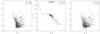 |
Fig. A.29. Same as Fig. 4 for vdBH 106. |
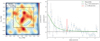 |
Fig. A.30. Same as Fig. 5 for vdBH 106. |
-
(a)
A color excess of E(B − V) = 0.30 was found to affect the cluster. This value agrees well with the maximum color excess provided by S&F2011, E(B − V) = 0.57, in this direction.
-
(b)
The absorption-free distance modulus of vdBH 106 was found to be 13.44 ± 0.36 mag, which places the cluster at a distance of d = 4.87 ± 0.81 kpc from the Sun.
In this region we found by applying the Anderson-Darling test that the parallax and proper motion distributions seem to belong to the same originating distribution, as shown in Fig. A.32. The high combined p-value makes the rejection of the null hypothesis difficult if not impossible
Although a trace of a sequence belonging to a typical old cluster is noticeable in Fig. A.31, we are cautious to confirm its nature. Clearly, deeper photometric observations (particularly in the U filter) are needed. Meanwhile, and assuming that it is a true object, vdBH 106 might be an old open cluster that is about 3.00 ± 0.80 × 10⁹ years old.
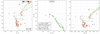 |
Fig. A.31. Same as Fig. 6 for vdBH 106. |
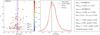 |
Fig. A.32. Same as Fig. 7 for vdBH 106. |
A.9. Ruprecht 88
RUP 88 is another potential cluster south of the Carina HII region. Like other objects in this paper, no obvious stellar grouping is perceived in the V image of Fig. 3. The overall stellar CMDs in Fig. A.33 show a scattered stellar distribution above G = 16 mag. From this magnitude down the common pattern of galactic disk stars takes place in the CMDs. The CCD in Fig. A.33 suggests that no blue and therefore young star is present in the region of RUP 88. In the range 0.2 < (B − V) < 0.8, a handful of stars might be reddened late B- types or A-F-type stars. The remainder of this diagram is a trace composed of A- to M-type stars.
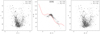 |
Fig. A.33. Same as Fig. 4 for RUP 88. |
As with other clusters in the present sample, when the spatial distribution of stars in the frame is analyzed, no clear stellar overdensity appears in the location where RUP 88 is assumed to be located. The contour plot in the left panel of Fig. A.34 shows a weak enhancement in star number from southwest to northeast of the frame extending northwest. Because it was difficult to state the position of the cluster center (if it exists), we asked ASteCA to inspect the region encircled in green in Fig. A.34, where a reasonable density profile could be found. The RDP is still noisy because of a rather low star number contained between the assumed cluster limits. The CMDs in Fig. A.35 show that only 42 stars with a wide range of probabilities remain inside the adopted cluster region after interlopers are removed, with no trace of a cluster sequence. The three photometric diagrams in Fig. A.35 confirm this point: only an amorphous distribution of stars that scarcely resembles a cluster main sequence is visible.
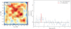 |
Fig. A.34. Same as Fig. 5 for RUP 88. |
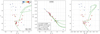 |
Fig. A.35. Same as Fig. 6 for RUP 88 with the (B − V) vs. (V − I) diagram instead of the (B − V) vs. (U − B) diagram. |
The Anderson-Darling test in the right panel of Fig. A.36 cannot separate the cluster population from the field region population for the three dimensions. The combined p-value for proper motions and parallaxes is hgih, suggesting that both samples come from the same population. The necessary requirement that there is a reasonable main sequence is not met, and combined with this result, precludes us from concluding that RUP 88 is a true cluster.
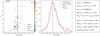 |
Fig. A.36. Same as Fig. 7 for RUP 88. |
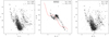 |
Fig. A.37. Same as Fig. 4 for RUP 162. |
A.10. Ruprecht 162
Placed to the southeast of the Carina HII region, the V image of the region in Fig. 3 where the cluster is assumed to lie shows a moderate number of stars resembling a stellar group placed northwest in the frame. At first glance, the CMDs in Fig. A.37 for all stars appear as if a cluster main sequence is emerging from the trace of the disk stellar distribution. In the middle panel of the same figure, the CCD splits into two star groups: one is mostly placed below the intrinsic line for 0.0 < (B − V) < 0.8 and resembles a strip of reddened blue stars (including early and late B-types and perhaps some A-type stars); the other group shows a distribution of F- to M-type stars that are strongly affected by reddening.
ASteCA detected an extended and irregular region northwest of the frame in Fig. A.38 (where the cluster is assumed to be). Because it is difficult to set a clear overdensity, we decided to focus on the ∼3 arcmin zone encircled in green in the left panel of Fig. A.38. The background mean stellar density is over 20 stars per squared arcminute, and at most, the overdensity is just 40 stars at the maximum. This unavoidably produces a noisy RDP (it is hard to establish a meaningful radius, and the stellar distribution throughout the zone is quite irregular).
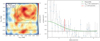 |
Fig. A.38. Same as Fig. 5 for RUP 162. |
The CMDs and CCD in Fig. A.39 show more than 200 dispersed stars after the field interlopers are removed. Most of the stars are assigned high probabilities. The large scatter in the CMDs and the high MP values that are assigned even to stars that are clearly not part of any cluster sequence point against the existence of a true cluster in the region. On the other hand, the cleaned CCD in the middle panel of Fig. A.39 shows a blue sequence of stars that suffer some internal color scatter followed by a tail of F- to K-type stars. Therefore this object might be more extended than assumed. ASteCA found the best fit with a synthetic cluster with the following properties:
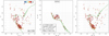 |
Fig. A.39. Same as Fig. 6 for RUP 162. |
-
(a)
The color excess affecting the cluster is E(B − V) = 0.54, well below the maximum value given by S&F2011, who estimated E(B − V) = 1.07.
-
(b)
The absorption-free distance modulus is 13.23 ± 0.10 mag, corresponding to a distance of d = 4.43 ± 0.20 kpc.
Anderson-Darling statistical test results are shown in the right panel of Fig. A.40. Parallaxes and proper motions PM(α) and PM(δ) in the location of RUP 162 and the surrounding field region do not seem to be different enough from each other as to be efficiently disentangled.
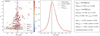 |
Fig. A.40. Same as Fig. 7 for RUP 162. |
Although weak enough, the probable main sequence in the panels of Fig. A.39 makes us cautious about leaving some possibility that RUP 162 is a true cluster of about 0.80 ± 0.20 × 10⁹ years. The hypothetical true entity of this young object is supported by the sudden gap along the main sequence at G = 16.5 mag and the high-probability stars on the red side that resemble traces of a pre-main sequence. We certainly only speculate about this, and that more and deeper observations are needed to conclude about RUP 162.
A.11. Lynga 15
This intriguing object is placed in Centaurus, southwest between Crux and the east border of Carina. More specifically, Lynga 15 is about 1° northeast of the star formation region SFR293.64-1.41 (Avedisova 2002). Like in many other cases already shown in the V images in Fig. 3, this region does not show at first glance any prominent stellar feature, although some stars are bright enough to attract attention to this place. However, the overall CMDs and CCD shown in Fig. A.41 are quite surprising because both CMDs depict an extended sequence (from G = 8 down to G = 15.5 mag) that emerges toward the left side of the main disk population trace. In the middle panel of the same figure, the CCD shows a strip of blue stars (0.0 < (B − V) < 0.0) accompanied by other, probable reddened, early-type stars, placed above (U − B) = 0.0. The picture shown in the three panels of Fig. A.41 induces us to think of Lynga 15 as a quite young open cluster.
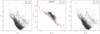 |
Fig. A.41. Same as Fig. 4 for Lynga 15. |
In turn, the ASteCA analysis of the spatial structure found an extended and irregular stellar density with no indication of a clear overdensity. The density map of the observed frame shows two very distinct stellar densities that are explained by the combination of observations made by two different telescopes, as detailed in Sect. 3 (same as NGC 4349). After many attempts to determine the place where the stellar membership probabilities reach the highest values, we adopted a radius of ∼2.9 arcmin and set the potential cluster center in the literature coordinates as indicated in the left panel of Fig. A.42. In this place, the RDP displays about 45 stars per squared arcminute peak above the stellar field density, as shown in the right panel of Fig. A.42. Even in this position, ASteCA yields a contradictory result because the selected probable members show a high dispersion, and as shown in the left and right panels of Fig. A.43, a probable cluster main sequence mostly composed of lower probability stars appears below approximately G = 17 mag. Above this visual magnitude, the main sequence vanishes, and only a handful of stars with rather high probability values remain, scattered in color index and magnitudes. This means that no upper cluster main sequence is evident in the clean CMDs. The CCD in the middle panel of Fig. A.43 contains a few blue stars with no counterpart in the CMDs. This might be explained in this way: throughout the surveyed region, there are blue stars (see the overall CCD in Fig. A.41) that compose a sort of blue plume in the respective CMDs, and some blue stars incidentally also appear in the potential cluster region after the ASteCA analysis (middle panel Fig. A.43). It is also possible, however, that Lynga 15 is an extended open cluster (even larger than the size of our frame), but the huge stellar gap above G = 17 mag cannot be explained in a CMD from a statistical point of view. In our opinion and from a photometric and spatial point of view, Lynga 15 is not an open cluster. The application of the Anderson-Darling test informs us that the properties of stars inside the adopted cluster radius and outside of it are similar, with a probability of ∼6% of mistakenly rejecting the null hypothesis that both samples arose from the same distribution.
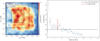 |
Fig. A.42. Same as Fig. 5 for Lynga 15. |
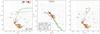 |
Fig. A.43. Same as Fig. 6 for Lynga 15. |
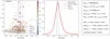 |
Fig. A.44. Same as Fig. 7 for Lynga 15. |
We conclude that Lynga 15 is not a true cluster, but a superposition of blue stars at several distances along the line of sight. This is not odd at all because this object is not far from the Galactic equator, therefore it is probable that blue stars are seen along the direction to this potential cluster.
A.12. Loden 565
Placed toward the west side of the Crux constellation, the V image in Fig. 3 of Loden 565 does not show any evident stellar grouping. Inspection of the CCD and CMDs in Fig. A.45 only suggests the presence of a dispersed stellar group down to approximately G = 15 − 16 mag. From this magnitude down, the overall CMDs show the common pattern of a Galactic disk stellar population, and nothing relevant is visible in the CCD in the middle panel of Fig. A.45, but a modest handful of probable slightly reddened late blue stars for (B − V) < 0.6.
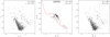 |
Fig. A.45. Same as Fig. 4 for Loden 565. |
ASteCA found an irregular overdensity at the northwest corner of the frame, as shown in the left panel of Fig. A.46. This is the only region in the entire field where a sudden increase in the star number per area unit is noticeable, showing about 40 stars per squared arcminute peak at its maximum in the right panel of Fig. A.46. When we searched for membership probabilities, only a small number of 60 stars remained inside the adopted radius, with higher probabilities scattered toward lower magnitudes. No clear main sequence is visible in the CMDs in Fig. A.47. None of the stars that occupy the CCD in the right panel of Fig. A.45 with 0 < (B − V) < 0.6, with some possibility of being reddened early-type stars, remain inside the adopted area after the membership analysis of ASteCA. The stars that ASteCA identified inside the adopted radius might be members of an old group, but we conclude that the photometric evidence is not at all conclusive. More extended and deeper observations are necessary. Previous estimates of the cluster parameters found for Loden 565 have been reported, by Kharchenko et al. (2005). These authors concluded that Loden 565 is a moderately young cluster placed at a distance of d = 0.65 kpc, affected by a mean reddening E(B − V) = 0.2 and a little older than 108 yr. The Kharchenko et al. (2005) atlas shows a poor fitting to very sparse available data. In addition, when the results from the Anderson-Darling test in the right panel of Fig. A.48 are inspected, it becomes evident that the cluster region is indistinguishable from the stellar background in terms of parallax and proper motion distributions, exactly like the clean CCD and CMDs show in Fig. A.47.
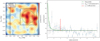 |
Fig. A.46. Same as Fig. 5 for Loden 565. |
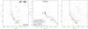 |
Fig. A.47. Same as Fig. 6 for Loden 565. |
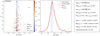 |
Fig. A.48. Same as Fig. 7 for Loden 565. |
In conclusion, Loden 565 is more probably a stellar fluctuation.
A.13. NGC 4230
This object belongs to the Centaurus region that lies very close to the upper border of Crux. The V image in Fig. 3 shows a modest stellar grouping near the high proper motion star HD 106826 with 8.8 mag. Nothing relevant is appreciable in the V image of the inspected zone, except for the star mentioned before. A highly scattered and diffuse stellar distribution resembling the stellar pattern of a Galactic disk appears in the general CCD and CMDs in the panels of Fig. A.49.
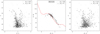 |
Fig. A.49. Same as Fig. 4 for NGC 4230. |
The spatial inspection performed by ASteCA detected a group of low stellar overdensities surrounding the central prominence, as shown in the left panel of Fig. A.50. The peak of the central overdensity shows that the number of stars per area unit is three times the mean of the background, and the respective RDP is provided in the right panel of Fig. A.50 suggests a radius of ∼2 arcmin. However, ASteCA yielded a frustrating result in terms of what it is expected for a real cluster when we analyzed the stellar properties inside and outside the overdensity. Only 46 stars remain inside the limits we adopted for NGC 4230. The synthetic cluster fit is found for the low-mass stars with the higher MP values. At this low number of members and with this high dispersion, we are unable to confidently separate the stellar population into objects belonging to a (putative) real open cluster and those belonging to the stellar field. The CCD and CMDs of these stars in Fig. A.51 reflect the physical situation because no main sequence is evident at all. At most, there is a sort of poorly defined giant stellar sequence whose meaning is dubious because there is no trace of a main sequence. The comparison with synthetic clusters performed by ASteCA mainly fit a group of stars with low brightness, as shown in the CMDs of Fig. A.51. This cluster was analyzed in Tadross (2011), who found an old 1.7 Gyr cluster, younger than our result of ∼8 Gyr, and at a much closer distance (1445 pc versus our result of about 4300 pc). Therefore the studies do not agree on the nature of this putative cluster.
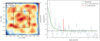 |
Fig. A.50. Same as Fig. 5 for NGC 4230. |
Results for the distribution of parallax values and proper motions for the cluster and field regions are shown in the right panel of Fig. A.52. The Anderson-Darling statistics reveals that the parallax and proper motion distributions are very similar to stars outside the cluster region.
The lack of a well-defined photometric sequence proper of an open cluster as demonstrated in Fig. A.51, together with the results from the statistical comparison is enough argument to exclude NGC 4230 as a true open cluster. It most probably is a random fluctuation of the stellar field.
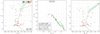 |
Fig. A.51. Same as Fig. 6 for NGC 4230. |
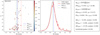 |
Fig. A.52. Same as Fig. 7 for NGC 4230. |
All Tables
Mean differences between APASS and the Carrasco transformation polynomials and our own photometry.
Fundamental parameters and parallax distances obtained for the confirmed and probable clusters.
All Figures
|
Fig. 1. Aladin DSS2 color image showing with white circles the positions of the clusters we survey here. The Galactic coordinates l and b are depicted by a green grid, and constellation limits for Carina, Vela, Centaurus, and Crux are plotted as yellow lines. |
| In the text | |
|
Fig. 2. Top row: differences between the APASS DR10 data for the V (left), B (center) magnitudes and (B − V) color (right) and our own photometry. Bottom row: same for Gaia DR2 data vs. our photometry. Details in the text. |
| In the text | |
|
Fig. 3. V images (charts) of the observed clusters (names inserted) ordered from top to bottom and from left to right by increasing longitude. Decimal α and δ coordinates for the 2000 equinox are indicated. North and east are also shown. |
| In the text | |
|
Fig. 3. continued. |
| In the text | |
|
Fig. 4. From left to right: G vs. (V − I), (B − V) vs. (U − B), and V vs. (B − V) diagrams for all the stars observed in the region of van den Bergh-Hagen 85. The red dashed line in the CCD shows the position of the ZAMS (Aller et al. 1982). Insets in each diagram contain the number of stars in the cluster region (Nclust, black circles) and in the surrounding field (Nfield, gray circles). |
| In the text | |
|
Fig. 5. From left to right, we present in the first panel a contour plot showing the position of the overdensity associated with vdBH 85. The green inner circle shows the cluster size, and the two black dashed-line squares enclose the region that ASteCA used to estimate the field stellar properties. The lower density values at the frame borders are an artifact of the kernel density estimate method that we employed to generate the density maps. Equatorial coordinates in decimal format are indicated. The color bar denotes the star number per square arcminute (linear scale). These values are slightly different from those in the panel to the right because they are obtained with a different method (nearest neighbors). The second panel shows the RDP as blue dots with standard deviations as vertical black lines. The King profile is shown as a dashed green line. The horizontal black line is the mean field stellar density. The vertical red line is the adopted cluster radius. |
| In the text | |
|
Fig. 6. From left to right: G vs. (V − I), (B − V) vs. (U − B), and G vs. (B − V) clean diagrams after field interlopers were removed by ASteCA over vdBH 85. The color of each star reflects its membership probability (MP). Corresponding values are in the color bar at the upper right corner in the G vs. (V − I) diagram (left) labeled MP. The CCD in the middle always shows fewer stars because of the U filter. The grid lines trace the edges of the three-dimensional photometric histograms we used to evaluate the likelihood function described in Sect. 4.2. The inset in the lower right corner in the G vs. (V − I) diagram shows the number of stars used by ASteCA to compare with synthetic clusters. The inset in the middle panel includes the final results for metallicity, log(age), E(B − V), the corrected distance modulus, and the total cluster mass provided by ASteCA. The green continuous line in the three diagrams is a reference isochrone. In particular, the green line in the CCD, middle panel, shows the most probable E(B − V) value fitting found by ASteCA. |
| In the text | |
|
Fig. 7. Left panel: distribution of the parallax for all stars with membership probabilities in the cleaned cluster region as a function of the apparent magnitude G (the vertical color scale shows the membership probability of the star) in vdBH 85. Horizontal bars represent the parallax errors as given by Gaia. The different parallax value fittings are shown by dashed lines of different colors: blue shows the Bayesian parallax estimate, green the ASteCA photometric distance, red the weighted average, and black the median (without negative values). Middle panel: normalized comparison between the parallax distributions inside (red line) and outside the cluster region (dashed black line). The frame at the right summarizes the distances in parsecs according to the Bayesian analysis (dBayes) and ASteCA (dASteCA), followed by the corresponding parallax value, Plx, and corrected distance modulus (μ0). Both fittings are indicated by the vertical blue and green dashed lines. The last four text lines in the right panel list the AD values for Plx, PM(α), and PM(δ), followed by the corresponding p-values, and finally, the combined p-value. |
| In the text | |
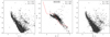 |
Fig. 8. Same as Fig. 4 for NGC 4349. |
| In the text | |
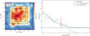 |
Fig. 9. Same as Fig. 5 for NGC 4349. |
| In the text | |
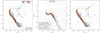 |
Fig. 10. Same as Fig. 6 for NGC 4349. |
| In the text | |
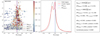 |
Fig. 11. Same as Fig. 7 for NGC 4349. |
| In the text | |
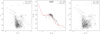 |
Fig. 12. Same as Fig. 4 for RUP 87. |
| In the text | |
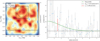 |
Fig. 13. Same as Fig. 5 for RUP 87. |
| In the text | |
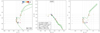 |
Fig. 14. Same as Fig. 6 for RUP 87. |
| In the text | |
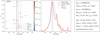 |
Fig. 15. Same as Fig. 7 for RUP 87. |
| In the text | |
|
Fig. 16. Left: ASteCA (photometric) vs. Bayesian (parallax) distances for the clusters listed in Table 4 that are confirmed to be real clusters. No bias correction was applied to the parallax data. The color bar at the right indicates log(age) values. Center: offset (ASteCA – Bayes) for distances expressed as parallax in miliarcseconds. Right: same as left plot, with bias corrections from Lindegren et al. (+0.029 mas). The cluster vdBH85 is included here; its distance value is estimated from the list of individual distances reported by Bailer-Jones et al. (2018). |
| In the text | |
|
Fig. 17. X − Y (upper panel) and X − Z (lower plane) projection of the true and probable clusters in our sample (open circles). The red squares enclose the youngest clusters in our list (see Table 4). The thick gray lines in the upper panel show the trace of the Perseus and Carina arms according to Vallée (2005). The position of the Sun is shown by a blue crossed circle. The dashed line in the lower panel depicts the Galactic equator. |
| In the text | |
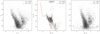 |
Fig. A.1. Same as Fig. 4 for vdBH 73. |
| In the text | |
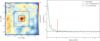 |
Fig. A.2. Same as Fig. 5 for vdBH 73. |
| In the text | |
|
Fig. A.3. Same as Fig. 6 for vdBH 73 with the (B − V) vs. (V − I) diagram instead of the (B − V) vs. (U − B) diagram. |
| In the text | |
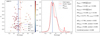 |
Fig. A.4. Same as Fig. 7 for vdBH 73. |
| In the text | |
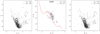 |
Fig. A.5. Same as Fig. 4 for RUP 85. |
| In the text | |
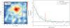 |
Fig. A.6. Same as Fig. 5 for RUP 85. |
| In the text | |
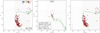 |
Fig. A.7. Same as Fig. 6 for RUP 85. |
| In the text | |
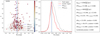 |
Fig. A.8. Same as Fig. 7 for RUP 85. |
| In the text | |
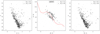 |
Fig. A.9. Same as Fig. 4 for vdBH 87. |
| In the text | |
|
Fig. A.10. Same as Fig. 5 for vdBH 87. |
| In the text | |
|
Fig. A.11. Same as Fig. 6 for vdBH 87. |
| In the text | |
|
Fig. A.12. Same as Fig. 7 for vdBH 87. |
| In the text | |
|
Fig. A.13. Same as Fig. 4 for vdBH 92. |
| In the text | |
|
Fig. A.14. Same as Fig. 5 for vdBH 92. |
| In the text | |
|
Fig. A.15. Same as Fig. 6 for vdBH 92. |
| In the text | |
|
Fig. A.16. Same as Fig. 7 for vdBH 92. |
| In the text | |
|
Fig. A.17. Same as Fig. 4 for TR 12. |
| In the text | |
|
Fig. A.18. Same as Fig. 5 for TR 12. |
| In the text | |
|
Fig. A.19. Same as Fig. 6 for TR 12. |
| In the text | |
|
Fig. A.20. Same as Fig. 7 for TR 12. |
| In the text | |
|
Fig. A.21. Same as Fig. 4 for vdBH 91. |
| In the text | |
|
Fig. A.22. Same as Fig. 5 for vdBH 91. |
| In the text | |
|
Fig. A.23. Same as Fig. 6 for vdBH 91. |
| In the text | |
|
Fig. A.24. Same as Fig. 7 for vdBH 91. |
| In the text | |
|
Fig. A.25. Same as Fig. 4 for TR 13. |
| In the text | |
|
Fig. A.26. Same as Fig. 5 for TR 13. |
| In the text | |
|
Fig. A.27. Same as Fig. 6 for TR 13. |
| In the text | |
|
Fig. A.28. Same as Fig. 7 for TR 13. |
| In the text | |
|
Fig. A.29. Same as Fig. 4 for vdBH 106. |
| In the text | |
|
Fig. A.30. Same as Fig. 5 for vdBH 106. |
| In the text | |
|
Fig. A.31. Same as Fig. 6 for vdBH 106. |
| In the text | |
|
Fig. A.32. Same as Fig. 7 for vdBH 106. |
| In the text | |
|
Fig. A.33. Same as Fig. 4 for RUP 88. |
| In the text | |
|
Fig. A.34. Same as Fig. 5 for RUP 88. |
| In the text | |
|
Fig. A.35. Same as Fig. 6 for RUP 88 with the (B − V) vs. (V − I) diagram instead of the (B − V) vs. (U − B) diagram. |
| In the text | |
|
Fig. A.36. Same as Fig. 7 for RUP 88. |
| In the text | |
|
Fig. A.37. Same as Fig. 4 for RUP 162. |
| In the text | |
|
Fig. A.38. Same as Fig. 5 for RUP 162. |
| In the text | |
|
Fig. A.39. Same as Fig. 6 for RUP 162. |
| In the text | |
|
Fig. A.40. Same as Fig. 7 for RUP 162. |
| In the text | |
|
Fig. A.41. Same as Fig. 4 for Lynga 15. |
| In the text | |
|
Fig. A.42. Same as Fig. 5 for Lynga 15. |
| In the text | |
|
Fig. A.43. Same as Fig. 6 for Lynga 15. |
| In the text | |
|
Fig. A.44. Same as Fig. 7 for Lynga 15. |
| In the text | |
|
Fig. A.45. Same as Fig. 4 for Loden 565. |
| In the text | |
|
Fig. A.46. Same as Fig. 5 for Loden 565. |
| In the text | |
|
Fig. A.47. Same as Fig. 6 for Loden 565. |
| In the text | |
|
Fig. A.48. Same as Fig. 7 for Loden 565. |
| In the text | |
|
Fig. A.49. Same as Fig. 4 for NGC 4230. |
| In the text | |
|
Fig. A.50. Same as Fig. 5 for NGC 4230. |
| In the text | |
|
Fig. A.51. Same as Fig. 6 for NGC 4230. |
| In the text | |
|
Fig. A.52. Same as Fig. 7 for NGC 4230. |
| In the text | |
Current usage metrics show cumulative count of Article Views (full-text article views including HTML views, PDF and ePub downloads, according to the available data) and Abstracts Views on Vision4Press platform.
Data correspond to usage on the plateform after 2015. The current usage metrics is available 48-96 hours after online publication and is updated daily on week days.
Initial download of the metrics may take a while.