| Issue |
A&A
Volume 632, December 2019
|
|
|---|---|---|
| Article Number | A20 | |
| Number of page(s) | 11 | |
| Section | The Sun | |
| DOI | https://doi.org/10.1051/0004-6361/201834735 | |
| Published online | 21 November 2019 | |
Measuring relative abundances in the solar corona with optimised linear combinations of spectral lines
Institut d’Astrophysique Spatiale, CNRS/Université Paris-Sud, Université Paris-Saclay, Bâtiment 121, Université Paris-Sud, 91405 Orsay Cedex, France
e-mail: This email address is being protected from spambots. You need JavaScript enabled to view it.
Received:
28
November
2018
Accepted:
30
September
2019
Abstract
Context. Elemental abundances in some coronal structures differ significantly from photospheric abundances, with a dependence on the first ionization potential (FIP) of the element. Measuring these FIP-dependent abundance biases is important for coronal and heliospheric physics.
Aims. We aim to build a method for optimal determination of FIP biases in the corona from spectroscopic observations in a way that is in practice independent from differential emission measure (DEM) inversions.
Methods. We optimised linear combinations of spectroscopic lines of low-FIP and high-FIP elements so that the ratio of the corresponding radiances yields the relative FIP bias with good accuracy for any DEM in a small set of typical DEMs.
Results. These optimised linear combinations of lines allow retrieval of a test FIP bias map with good accuracy for all DEMs in the map. The results also compare well with a FIP bias map obtained from observations using a DEM-dependent method.
Conclusions. The method provides a convenient, fast, and accurate way of computing relative FIP bias maps. It can be used to optimise the use of existing observations and the design of new observations and instruments.
Key words: techniques: spectroscopic / Sun: abundances / Sun: corona / Sun: UV radiation
© N. Zambrana Prado and É. Buchlin 2019
 Open Access article, published by EDP Sciences, under the terms of the Creative Commons Attribution License (http://creativecommons.org/licenses/by/4.0), which permits unrestricted use, distribution, and reproduction in any medium, provided the original work is properly cited.
1. Introduction
In order to understand the interactions between the Sun and the heliosphere and their impact on the celestial bodies living within the latter, we need to study the properties and the origin of the solar wind (SW), which shapes the heliosphere. Accurate plasma diagnostics of the SW and the corona, the uppermost layer of the solar atmosphere, and precise modelling of the solar magnetic field and plasma flows in the interplanetary medium are crucial when trying to determine the source regions of the SW (Peleikis et al. 2017). Indeed, the chemical composition of coronal plasma (the abundances of the different elements) may vary from structure to structure and in time (Feldman & Widing 2003) but it becomes fixed at low heights in the corona. Determination of the composition of the different structures would allow us to pinpoint the source of the SW by comparing and linking remote-sensing abundance measurements to in situ analysis.
Variations in coronal plasma abundances can be found in different types of structures such as active regions (Baker et al. 2013), jets, plumes (Guennou et al. 2015), and loops. These variations are linked to the first ionization potential (FIP; Saba 1995) of the different elements. Typically, in magnetically closed structures, the coronal abundances of elements that have a low FIP (< 10 eV) are enhanced in comparison to their photospheric abundances. This is not the case for elements with a higher FIP (for these elements the coronal and photospheric abundances are about the same). This anomaly is called the FIP effect (Pottasch 1964a,b), and it can be quantified by measuring the ratio of the coronal to photospheric abundance (the abundance bias, also referred to as FIP bias as it is FIP-dependent) of different elements. These anomalies do not only occur in the corona of the Sun but also in other stellar coronas, and an “inverse FIP effect” has even been detected in some of them (Laming 2015).
Being able to measure the FIP effect by remote sensing and comparing it to the in situ abundance diagnostics of the SW (von Steiger et al. 1997) can therefore allow us to determine the origin of the particles that arrive at a spacecraft (Brooks & Warren 2011). Having abundance maps produced systematically from all adequate ultra-violet (UV) observations would then help to obtain a better idea of how the SW is formed and how it unfolds in the interplanetary medium.
Different methods exist to determine photospheric abundances with remarkable accuracy even though there have been significant shifts in abundances of certain elements (oxygen in particular) throughout the years (Caffau et al. 2011; Schmelz et al. 2012; Grevesse et al. 2015; Scott et al. 2015a,b). Photospheric abundances do not vary with solar surface location or from one particular solar feature to another. On the other hand, coronal abundances, which are derived from UV spectroscopy, are much more difficult to measure accurately, as evidenced by the discrepancies between different measurements that were previously taken as a reference by the solar community (Schmelz et al. 2012). Even though the radiance of a UV spectral line emitted by an ion is proportional to its abundance, the latter is difficult to determine. This can be explained because many other parameters come into play, related to plasma conditions or to atomic physics, with high uncertainties for some of them.
First ionization potential biases are usually calculated either from the line ratio of two spectral lines (hereafter 2LR method) or following differential emission measure (DEM) analysis; both these methods can yield different results when used on the same data. In order to accurately obtain a FIP bias with the 2LR technique, both spectral lines have to be formed at very close temperatures, while using the DEM allows more flexibility in the choice of lines. However, the DEM is difficult to estimate accurately (Craig & Brown 1976; Judge et al. 1997; Landi et al. 2012; Testa et al. 2012a; Guennou et al. 2012), especially when trying to design an automated method.
In this paper we present a new method, developed with the aim to provide optimal determination of the abundance biases in the corona from a spectroscopic observation, even when the DEM cannot be precisely determined. The method is based on the DEM formalism and relies on linear combinations of spectral lines to get rid of the dependence on DEM inversion for FIP bias determination. We can think of several uses of such a method:
-
obtaining FIP bias maps from an existing observation that had not been specifically designed for this purpose;
-
designing an observation to obtain the best FIP bias map possible with a given instrument;
-
releasing the constraints on the list of spectroscopic lines required to build FIP bias maps, allowing the design of observations that perform more diagnostics simultaneously;
-
ultimately, helping to design the next solar or stellar UV spectrometers with FIP bias measurement capability.
In Sect. 2 we present the theoretical background for the method, which we present in Sect. 3. We test its accuracy and DEM independence and compare its results to those obtained by the line ratio technique using synthetic spectra in Sect. 4. We then apply our method to existing active region spectra obtained with the Hinode/EIS spectrometer and previously studied by Baker et al. (2013) in Sect. 5. We finish by discussing our results and the interest of the method in Sect. 6, where we also present our conclusions.
2. Theoretical background of FIP bias measurements in the corona
2.1. Contribution functions and DEM
In the tenuous and hot corona (in the so-called coronal approximation, Mason & Monsignori Fossi 1994; Landini & Monsignori Fossi 1990), the radiance of an optically thin spectral line at wavelength λij corresponding to the transition j → i of the X+m ions can be written as
 (1)
(1)
where νij is the frequency corresponding to the transition, Aij is the Einstein coefficient for spontaneous emission,  is the density of X+m ions in level j, and integration is over the line of sight.
In order to evaluate the quantities involved in Eq. (1) from the plasma parameters and atomic physics, this equation is frequently rewritten as
 (2)
(2)
where  is the elemental abundance in the corona relative to hydrogen, Ne is the electron density, and Cij(T, Ne) is the contribution function for the spectral line. This contribution function can be rewritten, in the simple case of a two-level ion, as
 (3)
(3)
In this equation, we recognise the relative level j population of ion X+m, the relative population of ionization stage +m of element X, and the hydrogen abundance relative to free electrons N(H)/Ne. The latter is usually taken as 0.83 in the corona as hydrogen and helium are almost completely ionized at T > 105 K.
The contribution function contains all atomic physics parameters that play a role in line formation, and it is different for each spectral line. In the case of many-level ions, Eq. (2) is still valid, but Cij has to be computed through more complex atomic physics models. In contrast, the distribution of  as a function of temperature along the line of sight is the same for all lines. However, as the spatial distribution of the plasma parameters T and Ne along the line of sight is lost in integration, while the usual shape of contribution functions (with a strong dependence on temperature and a weaker dependence on density for most spectral lines) tends to “select” some temperature range for a given spectral line, it is useful to substitute T for z in the integral, by writing
 (4)
(4)
where the DEM can be defined by
 (5)
(5)
in the simple case where temperature is a strictly monotonous function of the position along the line of sight.
Different methods exist to determine the DEM from the observed radiances in several spectroscopic lines using integral inversion methods. However, this is not an easy task as this method has many limitations (Craig & Brown 1976; Laming 2015; Landi et al. 2012). For most DEM determination techniques, a previous measurement of the density is needed. The insufficiency of the available data as well as the intrinsic nature of DEM inversion make it a difficult, ill-constrained problem that is very poorly conditioned in the density dimension (Judge et al. 1997; Testa et al. 2012a). Through the application of some of these inversion methods to synthetic data, one finds that the general shape of the DEM is not always well retrieved and the finer details are not always well resolved (Testa et al. 2012a). As in any such problem, different DEM(T) functions can equally reproduce the observed radiances. Furthermore, when dealing with synthetic observations of multithermal plasma, DEM inversion fails to find a good match with the “true” DEM (Testa et al. 2012a) and isothermal DEM inversion solutions for a multithermal plasma are biased to specific temperature intervals, for a given set of spectroscopic lines (Guennou et al. 2012).
We now take a quick look at the current FIP bias-determination methods based on this formalism.
2.2. First ionization potential bias determination
Let us consider two spectroscopic lines emitted by ions of two different elements: XLF that has a low FIP (LF, < 10 eV) and XHF that has a high FIP (HF). The radiance of the considered spectral line of the low-FIP and high-FIP elements is denoted ILF and IHF, respectively.
Assuming that abundances are uniform along the relevant part of the line of sight, in the corona, we can write Eq. (4) for both lines as
 (6)
(6)
 (7)
(7)
where  are the coronal abundances for each element, CLF and CHF are the contribution functions for the lines of the low-FIP and high-FIP elements, respectively, and ⟨a, b⟩ ≡ ∫a(T) b(T) dT is a scalar product.
Introducing the photospheric abundance  and the FIP bias
  for element X, the ratio of line radiances becomes
 (8)
(8)
When the DEM can be inferred from observations and the contribution functions computed from atomic calculations, the relative FIP bias between high-FIP and low-FIP elements can then be derived from Eq. (8) using the observed radiances and assuming the photospheric abundances:
 (9)
(9)
This ratio is simply the low-FIP element abundance bias fXLF if we consider that fXHF = 1.
In practice, the required DEM inversion itself is sensitive to FIP bias, especially because DEM inversion often involves iron lines, a low-FIP element. This sensitivity can however be used as a way to determine the FIP bias, as in e.g. Baker et al. (2013), Guennou et al. (2015). A short step-by-step description of their process is presented in Appendix A.
Another method for FIP bias determination is the 2LR method, which does not involve DEM inversion. When two spectral lines, one from a low-FIP ion and another from a high-FIP ion, can be chosen so that their contribution functions are very close (at some factor which can then be approximated by max(CLF)/max(CHF)), the ratio of the scalar products in Eq. (8) becomes almost independent from the DEM, and the relative FIP bias becomes
 (10)
(10)
This is simply the ratio of the radiances multiplied by some constant factor.
Of course, finding such adequate line pairs of low-FIP and high-FIP elements with similar contribution functions is difficult and not always possible given the observational constraints. Furthermore, no two contribution functions are exactly the same, so there is some hidden dependence on the DEM, and this method is then less accurate than using Eq. (9) after inversion of the DEM.
However, as mentioned above, DEM inversion is a difficult problem, and therefore a FIP bias determination that would not rely on DEM inversion, like the 2LR method, but that would also be more accurate than the two-line ratio method would be very convenient. This is the main motivation for the development of our method.
3. A new way of measuring the FIP effect: the linear combination ratio method
3.1. Light bulb
For some elements, as mentioned above, we can make relative abundance diagnostics without knowing the DEM, by using radiance ratios of the spectral lines of a low-FIP element and a high FIP element, provided they both have very similar contribution functions. Such lines are not always observable however, or their contribution functions are not close enough. Our idea is therefore to generalise this technique by using linear combinations of lines so that the corresponding contribution functions for low-FIP and high-FIP elements are a better match.
We start by defining two radiance-like quantities that would be the analogues of the radiances of Eqs. (6) and (7), as linear combinations of radiances from individual lines of low-FIP and high-FIP elements:
 (11)
(11)
 (12)
(12)
Please note that the normalization by photospheric abundances here is only a matter of convention. Using Eq. (4), these quantities become
 (13)
(13)
 (14)
(14)
If the FIP biases of all used low-FIP elements are the same (and equal to fLF), and the FIP biases of all used high-FIP elements are the same (and equal to fHF), the ratio of the radiance-like quantities is
 (15)
(15)
 (16)
(16)
where the low-FIP and high-FIP contribution functions have been defined by
 (17)
(17)
 (18)
(18)
then the relative FIP bias is
 (19)
(19)
This is analogous to Eq. (10) but for the linear combinations of radiances and of contribution functions.
3.2. Finding the optimal linear combinations
So that the relative FIP bias can be retrieved from observations without determining the DEM, our first idea was to optimise the linear combination coefficients so that the following cost function is minimised:
 (20)
(20)
where the distance is defined from the scalar product: ||a||2 ≡ ⟨a, a⟩. If there is no difference between 𝒞LF and 𝒞HF, the relative FIP bias from Eq. (19) is indeed simply ℐLF/ℐHF. However, if differences remain, especially in the wings of the linear combinations of contribution functions, the result remains sensitive to the DEM.
We therefore decided to look at the problem from a different angle but with a similar approach. Instead of building the cost function ϕ from the distance between the contribution functions as in Eq. (20), we came back to Eq. (16) and built a new cost function in such a way that after optimisation the ratio ⟨𝒞LF, DEM⟩/⟨𝒞HF, DEM⟩ would become as close to 1 as possible for any DEM. As we do not want to compute the DEM in each pixel, this means that we have to choose a set (DEMj)j of “reference” DEMs that would be representative of the DEMs in the map, and we then define the cost function as
 (21)
(21)
This is simply the L2 distance between vector
 (22)
(22)
and vector (1)j.
Through the minimisation of ϕ we obtain the coefficients αi and βi. Provided that the set of DEMs used to define the cost function from Eq. (21) is adequate, we then have ψDEM = ⟨𝒞LF, DEM⟩/⟨𝒞HF, DEM⟩≈1 in each pixel and following Eq. (19) the relative FIP bias can be simply retrieved as
 (23)
(23)
This allows us to build relative FIP bias maps from spectroscopic observations without having to determine the DEM in each pixel. We call this method Linear Combination Ratio (LCR) method.
We note that the 2LR technique, as defined by Eq. (10), is a special case of a linear combination and can be expressed with the same formalism as the LCR method: a single line from a low-FIP element is chosen along with a single line from a high-FIP element, and the linear combination coefficients are
 (24)
(24)
for the single LF and HF lines, instead of being the result of an optimisation.
3.3. Implementing the LCR method
We have developed a Python module1 to compute the optimal linear combinations of spectral lines and to use them to compute relative FIP bias maps from observations.
We describe the different steps to apply the method to observations of UV spectra in the following.
3.3.1. Selection of the spectral lines
We first need to choose the spectral lines that we want to use. This has to be done by hand, and depends on the lines available for a given observation, instrument, or wavelength range. The following criteria should be taken into consideration:
– The lines have to verify the coronal approximation (see Sect. 2.1).
– They have to form at coronal temperatures; if they form at lower temperatures opacity effects would have to be taken into account.
– The observed signal-to-noise ratio of each line radiance has to be sufficient. The noise in the observed radiance of a weak line propagates indeed to the corresponding linear combination of radiances, especially when it is amplified by a large coefficient in the linear combination.
– Blended lines have to be avoided or de-blended so that the true spectral line radiance is used.
– The atomic physics for the spectral lines has to be well known. Examples of some of the problems that one might encounter are an underestimation of the observed flux in the 50−130 Å wavelength range (Testa et al. 2012b) or anomalous behaviour for ions of the Li and Na isoelectronic sequences for which the atomic physics models tend to underestimate line radiance (Del Zanna et al. 2001; Sect. 7.4 of Del Zanna & Mason 2018). The quality of the atomic data will depend on the database chosen. For the purpose of this paper, we use CHIANTI (version 9.0, previous versions described in Dere et al. 1997; Del Zanna et al. 2015) through the ChiantiPy Python package (version 0.8.5), but in principle another database can be used.
– The maximums of the contribution functions of all lines should be at similar temperatures so that we do not mix abundances at various heights.
3.3.2. Computation of the contribution functions
We use the CHIANTI atomic physics database to compute the contribution functions. We also use it to retrieve information about each spectral line, such as typical photospheric abundance, FIP of the element, and upper and lower levels of the transition. Furthermore, for the cases when density maps can be obtained, for example when using a radiance ratio between a pair of lines with different density sensitivities, we compute these contribution functions on a grid of temperatures and densities.
3.3.3. Determination of the optimal linear combinations
Lines are first separated into two subsets, LF for lines from low-FIP elements and HF for lines from high-FIP elements. We then minimise the cost function ϕ defined by Eq. (21) using a very simple set of DEMs, constituted by the typical DEMs provided by CHIANTI for an active region (AR), a coronal hole (CH), and the quiet Sun (QS). For this minimisation, we use the Nelder & Mead (1965) optimisation implemented in the SciPy library (Jones et al. 2001). As a first guess for the coefficients for each linear combination, we use the median of the maximums of the contribution functions divided by each of these maximums. The optimisation then yields a set of optimal coefficients, (αi)i ∈ LF and (βi)i ∈ HF. These coefficients can be optimised for the density grid mentioned in Sect. 3.3.2 if required; we would then obtain optimised linear combination coefficients that are a function of density.
3.3.4. Determining the relative FIP bias
Once we have the coefficients of the linear combinations, we can compute the linear combinations of radiances ℐLF and ℐHF in each pixel, and then immediately obtain the relative FIP bias fLF/fHF from Eq. (23). If a density map can be obtained for the observation, we can compute the FIP bias in each pixel using the linear combination coefficients best suited for that particular pixel depending on its density (the density dependence of the ratio of the radiances is further discussed in Appendix B).
4. Testing the method with synthetic radiances
In this section we test the LCR method by applying it to maps of synthetic radiances, so that we control all parameters precisely (in particular the abundances). We also test the 2LR method with the same criteria for comparison.
The test case consists in a uniform abundance map for any given element, combined with a data cube of DEMs, as detailed below. Using both these inputs and atomic physics, we can build “synthetic” radiances, meaning that they are computed rather than observed. The test is considered successful for a given FIP bias determination method if the output relative FIP bias map is consistent with the input elemental abundance maps, both in uniformity and in value. The test has four main steps, detailed below:
1. We derive a DEM cube from the AIA observation. This is for the sole purpose of producing synthetic radiances, for which we have control over all parameters, while the DEMs are representative of different real solar regions.
2. Using CHIANTI for the contribution functions and the derived DEMs, we calculate the synthetic radiances. We assume different uniform abundances for different elements.
3. We determine the optimal linear combination coefficients for the LCR methods, and the coefficients for the 2LR method.
4. We use these coefficients to retrieve the FIP bias in each pixel assuming Eq. (23) is verified. If this is the case, the retrieved FIP bias map should be uniform.
4.1. Synthetic radiance maps
We start by computing emission measure2 (EM) maps using the Cheung et al. (2015) code (version 1.001), which is available in the SDO/AIA package in SolarSoft. This particular EM inversion method finds a sparse solution, that is, it uses a minimum number of basis functions to produce an EM(T) compatible with the observations.
We chose an observation of the Atmospheric Imaging Assembly (AIA; Lemen et al. 2012) instrument aboard the Solar Dynamics Observatory (SDO; Pesnell et al. 2012), on June 3, 2012, close to the maximum of solar activity, so that the coronal emission is inhomogeneous. The Sun in this particular day presented various ARs and a large CH at the centre. As shown in Fig. 1, we select two separate regions of interest, one being centred on an AR, and the other centred on a CH. We aligned the images from the different detectors and divided each of them by their corresponding exposure time before doing the EM computations. The histograms of the EMs we obtain are shown in Figs. 2 and 3.
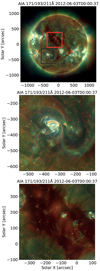 |
Fig. 1. Top panel: composite map of the solar corona on June 3, 2012, in the 171 Å (red), 193 Å (green), and 211 Å (blue) channels of the AIA instrument aboard SDO. The black and red squares correspond to the regions of interest used for testing the method, and are centred on an AR and a CH, respectively. Middle panel: zoom on the AR region of interest (black square in top panel). Bottom panel: zoom on the CH region of interest (red square in top panel). |
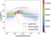 |
Fig. 2. Histogram of the EM(T) values in the first region of interest (black square) of Fig. 1. The colour scale and the size of the points correspond to the number of pixels containing an EM of a given value at a given temperature. We have also traced in full lines the typical EMs from CHIANTI that we use to optimise the cost function (Eq. (21)). The red line corresponds to an active region, the blue line to the quiet Sun and the yellow line to a coronal hole. |
We selected lines available in the observations used by Baker et al. (2013), as in Sect. 5 we use the same observational data as these authors to compare the LCR method results to their results. Eight lines were chosen following the criteria of Sect. 3.3.1 and are listed in Table 1. The temperature range of their maximums of formation goes from 1 MK to 2 MK. They include five iron lines, two silicon lines, and one sulfur line; iron and silicon are low-FIP elements, and, like Baker et al. (2013), we consider sulfur to be high-FIP. We further select Si X 258.374 Å as low-FIP line for the 2LR method.
Spectral lines used to perform the calculations.
We then create the required synthetic radiance maps using Eq. (4), assuming the relative abundance ratios presented in Table 2, which provide the “ground truth” for the FIP biases we obtain using both methods. The abundances we assume here are uniform3 over the regions of interest, and we take their values from Schmelz et al. (2012) for the corona and Grevesse et al. (2007) for the photosphere; these values and resulting relative FIP biases are presented in Table 2.
First ionization potential of the elements used for the tests, their coronal and photospheric abundances taken from Schmelz et al. (2012) and Grevesse et al. (2007), and the corresponding abundance bias relative to sulfur.
4.2. Optimisation of the linear combinations of lines
We present in Fig. 4 the contribution functions for the spectral lines listed in Table 1. All contribution functions were computed assuming a density of 108.3 cm−3. In the top panel of Fig. 4, we show the contribution functions of both lines used for the 2LR method, normalized by their maximum. As we can see, they are similar in shape from low temperatures until the maximum of both functions, but for higher temperatures they start to differ from one another significantly. In the bottom panel of Fig. 4, we present the contribution functions of all the lines we use to test the LCR method. They all have different shapes and values. Not all of them start at low temperatures, as ions with a high degree of ionization are formed only at higher temperatures.
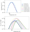 |
Fig. 4. Top: normalized contribution functions of the lines used for the 2LR method. Bottom: contribution functions of the lines used for the LCR method. All the contribution functions were calculated assuming a constant density of 108.3 cm−3. |
After choosing the lines and computing their contribution functions, we determine the optimal linear combination of these lines for the LCR method (Sect. 3.3.3). The reference EMs that we use for the optimisation are plotted on Figs. 2 and 3. These are available in the CHIANTI database and correspond to typical EMs for a coronal hole, an active region, and the quiet Sun. The resulting coefficients are included in Table 1. For the 2LR method, we use the inverse of the maximum of the contribution functions of the Si X and of the S X lines as values for the (single) α and β coefficients, respectively, therefore allowing the use of the same formalism as for the LCR method.
In particular, we can compute the cost function defined in Eq. (21) for both the LCR method (following optimisation) and the 2LR method, as shown in Table 3. In this table we also give the components of vector ψ defined in Eq. (22), which ideally would all have to be equal to 1 so that the cost function ϕ would be zero. The values in this table already show that the optimisation made in the LCR method yields much better values for the cost function, as well as for each of the ψ components, compared to the same quantities for the line coefficients chosen for the 2LR method. This means that Eq. (19) would give very good estimates of the relative FIP bias for any of the three reference DEMs that we use. It is a first indication that the LCR method could work well.
4.3. First ionization potential bias maps obtained from the synthetic radiances
Applying Eq. (19) to the synthetic radiance maps, we now obtain maps of the relative FIP bias for both LCR and 2LR methods.
We present the results for the first region of interest (black square in Fig. 1) in Fig. 5. The top left panel of this figure clearly shows that we do not retrieve a uniform relative FIP bias using the 2LR method, as confirmed by the standard deviation of the FIP bias (0.15) and the corresponding histogram (bottom left). Furthermore, the histogram peak at about 1.51 is far from the imposed value for the relative FIP bias between the two elements used, silicon and sulfur (1.82). This could be because the normalized contribution function of the S X line goes well over (up to a factor 3.6) that of the Si X line in the temperature range at which the EM peaks (log T = 6.3 − 6.4), as we can see in Fig. 4.
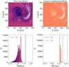 |
Fig. 5. Results of FIP bias determination using the 2LR (left) and LCR (right) methods on the synthetic radiances in the first region of interest (black square) of Fig. 1: relative FIP maps (top) and their corresponding histograms (bottom), with matching colour scales. The DEM inversion code was not able to find a satisfactory solution in the pixels depicted in white. The vertical lines in the histograms correspond to the imposed uniform values of the relative FIP bias (for each of the low-FIP elements; see Table 2) that should ideally be retrieved. |
The LCR method gives a much more uniform map (top right panel), as confirmed by the corresponding histogram (bottom right) that has a standard deviation of 0.03, a factor of five smaller than that obtained with the 2LR method. Almost all obtained values are between the relative FIP biases for Fe and Si, as we discuss in Sect. 4.4. This histogram peaks at 1.87. These results show the accuracy of the linear combination ratio method.
In order to test if these results can be reproduced in regions other than an AR, we perform the same test in the red square of Fig. 1. We can see in Fig. 1 that this region contains very different structures than the first one, as the second region includes part of a CH. In the results, presented in Fig. 6, we can see that the LCR method performs again better than the 2LR technique. We obtain a distribution of relative FIP biases peaking at 1.58 (with a standard deviation of 0.1) for the 2LR method, still very far from 1.82, and a distribution peaking at 1.9 (with a standard deviation of 0.015) for the LCR method. In this case, almost all values are again between the relative FIP biases for Fe and Si.
The LCR results are very close to the imposed FIP biases in both regions even though their EMs are very different (and each region already contains pixels with different EMs). This shows that the LCR method works properly and does not require prior knowledge of the DEM.
4.4. Understanding the remaining non-uniformity in maps
As the assumed FIP bias map (the ground truth for the test) was uniform, the non-uniformity in the result FIP bias map is a measure of the error in the FIP bias given by the tested method (LCR or 2LR) for this test setup (for the spectroscopic lines, reference EMs, and EM map used for the test). Other sources of error that cannot be assessed with such a test are discussed in Sect. 6.
Even though the relative FIP bias values obtained in this test with the LCR method have a standard deviation of 0.02 and 0.03 only in both regions of interest, the 1st and 99th percentiles are 1.78 and 1.88 respectively. Although much better than for the 2LR method, the non-uniformity of the FIP bias is still significant, and we ought to understand possible sources of the remaining non-uniformity in our test FIP bias maps.
Optimisation residuals. Even after the optimisation, the residuals of the cost function Eq. (21) are not zero (Table 3). From Eq. (22), one understands that these residuals come from the fact that the products 𝒞LF(T) EM(T) and 𝒞HF(T) EM(T) for the different EMs used for the optimisation are not close enough. We trace these products for the three reference EMs we used and for both methods in Fig. 7.
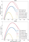 |
Fig. 7. Products between the EM and the contribution functions (𝒞LF, solid lines, and 𝒞HF, dashed lines), as functions of the temperature for both methods, using the coefficients in Table 1. Different colours correspond to different EMs from CHIANTI. |
Above log T = 6.2, both LF and HF curves have the same shape for the LCR linear combinations, whereas this is not the case for the 2LR method. The yellow curves in the top panel of Fig. 7 show that, with the AR EM, the 2LR method would overestimate the S X contribution in the log T ∈ [6.2, 6.6] range by a factor up to 3.6. Above log T = 6.5, the S X contribution would be underestimated for both methods, but we are far from the peak which means that the contribution of the radiance at these high temperatures might not contribute much to the overall observed radiance.
After integration over T, the resulting ⟨𝒞, EMAR⟩ is higher for S than for Si, corresponding to the fact that ψAR is 24% lower than 1 (see Table 3). This is consistent with the strong underestimation of the FIP bias that is obtained following this test in active regions with the 2LR method, as seen in Figs. 5 and 6.
In contrast, for the LCR method, the mean distance between the LF and HF curves in Fig. 7 is much smaller than for the 2LR method. This is measured, after integration over T, by the values of ψj in Table 3: these values are very close to 1.
Overall, this means that the LCR method performs better than the 2LR method in the range of temperatures including the peak of the mean coronal DEM.
Cost function residuals for real DEMs. The analysis of the cost function residuals in the previous paragraph is for the set of reference EMs that were chosen for the optimisation. However, the DEMs in the map are different. With real observations, we cannot measure the impact of this choice unless we perform a thorough DEM analysis, but this is not an issue in the case of the synthetic observations we produced for our tests in this section.
By applying Eq. (22) to the EM we used to produce synthetic radiances in every pixel, we can then retrieve the uncertainty linked to the arbitrary choice of reference EMs. In other words, we can determine through this calculation how far ψEM is from one for the EM in every pixel. As we can see in Eq. (23), this factor determines if we over- or underestimate the relative FIP bias. In both test regions, ψEM is 1 ± 0.01, meaning that in our case the impact on the FIP biases of the fact that the EMs in the map are not those chosen for the optimisation of the LCR coefficients is 1%. Therefore, the optimal linear combinations seem to be very well adapted to these EMs even though they were not optimised for them specifically.
Use of different low-FIP elements. As most values obtained in the test with the LCR method are between the relative abundance biases of Si (1.82) and Fe (2.05), one reason for the remaining non-uniformity in the maps could be the use of lines of LF elements with different abundance biases, while we assumed from Eq. (16) that they were the same. To assess this potential reason, we determine how much the spectral lines of each element are contributing to the total linear combination of LF elements in order to fit as best as possible to our HF line.
In our case, we show in Fig. 8 the respective contributions of the Fe and Si lines to the 𝒞(T) EM(T) product for the LF linear combination of the LCR method and for the AR EM (for which the differences in the log T ∈ [6.2, 6.5] interval were most noticeable for the 2LR method, as discussed above). The relative contributions of the Fe and Si lines depend on temperature. This is true in this case, with the AR EM, but these proportions will vary for different DEMs. As a result, for any given DEM, the FIP bias given by the LCR method will be closer to that of one element or the other, which can explain a part of the dispersion seen in the histograms of Figs. 5 and 6.
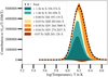 |
Fig. 8. Contributions of the different spectroscopic lines to the 𝒞LF(T) EM(T) product as a function of temperature for the CHIANTI AR EM. The total (dotted line) corresponds to the full red line in the bottom panel of Fig. 7. Here, Fe and Si line contributions are shown in ocher-red and blue-green colours, respectively. We separate the positive and negative contributions to the total. |
5. Determining FIP bias from observations
We applied the LCR method to spectroscopic observations of a sigmoidal anemone-like AR inside an equatorial CH that has previously been studied (including plasma composition) in Baker et al. (2013). A full description of the evolution of this AR from the 11 to the 23 October, 2007, including measurement of multi-temperature plasma flows, is presented in Baker et al. (2012). We focus on a single raster observation lasting 2.25 h that was carried out with the EIS spectrometer (Culhane et al. 2007) aboard Hinode (Kosugi et al. 2007) on October 17, 2007, at 2:47 UT.
Baker et al. (2013) used the method described in Appendix A in order to retrieve FIP bias maps. These latter authors used ten Fe lines in order to infer the EM from line radiances. They scaled this EM to accurately reproduce the radiance of the same Si X line that we used previously for the 2LR method (see Table 1). They then simulated the radiance of the same S X line that we used in the previous section and compared it to the observed radiance. The ratio gives a FIP bias map, reproduced in the left panel of Fig. 10.
In our analysis, we start by applying standard SolarSoftware EIS data-reduction procedures to the data, including correcting for dark current hot, warm, and dusty pixels, cosmic rays, slit tilt, CCD detector offset, and orbital variations. The obtained calibrated spectra were then fitted by single (or double, when necessary) Gaussian functions, and we computed integrated radiances for all lines.
We then selected the lines to be used for the LCR method, using the criteria from Sect. 3.3.1. This gives the five Fe lines, the two Si lines, and the S line listed in Table 1. We calculated the density of this AR using the Fe XIII λ 202.02 and 203.83 line pair diagnostic. This density map is plotted in Fig. 9. We then determined the optimal coefficients to use in each pixel using this map. In the case of this EIS observation, all the selected lines have strong radiances and are fairly isolated in the spectrum. However, among the EIS windows of this observation, only one line of an element considered as HF fits all our selection criteria. As a result, the set of HF lines is reduced to a single line (as in Sect. 4).
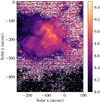 |
Fig. 9. Map of the logarithm of the density in cm−3 obtained for the observation on October 17, 2007, from EIS spectra. We used the Fe XIII λ 202.02 and 203.83 line pair to calculate this density map. In the white pixels, fitting of the EIS lines failed. The density value of each pixel allows us to compute the optimal linear combination of lines to be used to determine the FIP bias in those pixels. |
The results of the LCR method on this observation are presented in the right panel of Fig. 10. The FIP bias maps (from Baker et al. 2013 and from the LCR method) display similar FIP bias structures. The distributions of FIP bias values (bottom panels of Fig. 10) peak at 1.11 and 1.29. The correlation between both sets of values (Fig. 11) also shows that the LCR values are higher overall than the Baker et al. (2013) values. However, we do not expect a perfect correlation as the real FIP bias values in this region are not known. We find that the LCR FIP bias map provides useful information on the FIP biases in the coronal structures in the field of view, which is remarkable given that it was produced without any DEM inversion.
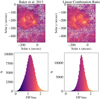 |
Fig. 10. First ionization potential bias maps obtained with different methods and the corresponding histograms. Left panel: FIP bias map obtained following DEM inversion (adapted from Baker et al. 2013). Right panel: FIP bias map obtained using the LCR method. In the white pixels, the fitting of the EIS lines we performed failed. In both FIP bias maps we only plot the pixels where our fitting was successful. |
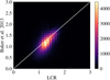 |
Fig. 11. Two-dimensional histogram of the FIP bias values of Baker et al. (2013) and those obtained using the LCR method. The white line is the first bisector, where both values are equal. |
6. Discussion
Some sources of errors that could be identified from the non-uniformity in the test result in Sect. 4 have already been discussed in Sect. 4.4: the cost function residuals for the reference DEMs and for the real DEMs in the map, and the assumption that all LF (or HF) elements used have the same abundance bias. The cost function residuals for the real DEMs could be reduced by using a more comprehensive set of reference DEMs, or a set that would be more adapted to the observation; but the latter would require better knowledge of the DEMs in the observation, and we wanted to avoid inverting DEMs. The tests we have done show however that the residuals are in practice small for real DEMs given the set of three reference DEMs that we have chosen for the optimisation, and so this set is sufficient.
In regards to the mixing, in the same group (LF or HF) of spectroscopic lines from different elements with different abundance biases this is a matter of compromise. As one can see in Fig. 8, for the set of lines that we have chosen (the same as the ones available in the observation analysed by Baker et al. 2013 and re-analysed in Sect. 5), using only Si lines would not have allowed us to fit the LF and HF 𝒞LF(T) EM(T) products, especially in the most relevant temperature interval (close to the DEM peak). The Fe lines provide a better fit, and subsequently a smaller value for the optimised cost function. This gives in the end a more accurate FIP bias determination, although the assumption that all abundance biases are the same for all LF or HF elements has not been verified; this must be checked on a case-by-case basis, depending on the elements giving the available spectral lines, along with their behavior with respect to the FIP effect.
As in any UV spectroscopic analysis, other uncertainties come from radiometry (inaccurately measuring the line radiances, e.g. because of calibration or line blends), atomic physics (imprecise atomic data for computing the contribution functions; not taking into account effects such as those from non-Maxwellian distributions or from non-equilibrium of ionization, when required) and radiative transfer (opacity and scattering).
7. Conclusion
Here, we present the LCR method, developed with the aim to provide optimal determination of the relative FIP biases in the corona from spectroscopic observations without the need to previously determine the DEM. This technique relies on linear combinations of spectral lines optimised for FIP bias determination. We developed a Python module to implement the method that can be found online4.
Using two linear combinations of spectral lines, one with low FIP elements and another with high FIP elements, we tested the accuracy of the method performed on synthetic observations: these tests show that the method does indeed perform well, without prior DEM inversions. We then applied it to Hinode/EIS observations of an active region. We obtained FIP bias structures similar to those found in the same region by Baker et al. (2013) following a DEM inversion.
Once the optimised linear combination coefficients have been determined for a given set of lines, if radiance maps can be obtained in these lines, the LCR method directly gives the corresponding FIP bias maps, in a similar way to the 2LR method, but with better accuracy. This makes the method simple to apply on observations containing a pre-defined set of lines, with a potential for automation.
Hopefully, producing such FIP bias maps semi-automatically will allow non-specialists of EUV spectroscopy to obtain composition information from remote-sensing observations and compare it directly with in-situ data of the SW. This method could also allow better exploitation of observations not specifically designed for composition studies, and an optimal design of future observations. We plan to apply the method to the future Solar Orbiter/SPICE spectra to prepare the observations and analysis of the SPICE data.
The EM is the DEM(T) integrated over temperature bins, of width assumed to be Δlog T = 0.05 in this section. Then ⟨𝒞, DEM⟩ ≈ ∑i𝒞(Ti) EM(Ti), where the sum is over the temperature bin centres.
Uniformity allows an easy comparison between the obtained FIP bias maps and the ground truth; however, any map could be assumed for the test, as the test (from synthetic radiances to FIP bias maps) gives a result that is proportional to the initial FIP bias in each pixel, as long as all the LF or HF element abundance vectors are collinear.
If one wants to compute the FIP bias for another low-FIP element (e.g. Si, when the DEM was computed using Fe lines), the inferred DEM is rescaled so that it reproduces the observed radiance of a line of that element.
Acknowledgments
The authors thank Mark Cheung for the SDO/AIA DEM inversion code, Deborah Baker for providing the FIP bias map data, and Giulio Del Zanna, Susanna Parenti, and Karine Bocchialini for their comments. The idea for this work came following a presentation by Hardi Peter at the Solar Orbiter joint SPICE-EPD-SWA meeting in Orsay in November 2015. AIA is an instrument on board SDO, a mission for NASA’s Living With a Star program. NZP thanks ISSI for support and participants to the ISSI team n. 418 “Linking the Sun to the Heliosphere using Composition Data and Modelling” led by Susanna Parenti. Hinode is a Japanese mission developed and launched by ISAS/JAXA, with NAOJ as domestic partner and NASA and STFC (UK) as international partners. It is operated by these agencies in cooperation with ESA and NSC (Norway). CHIANTI is a collaborative project involving George Mason University, the University of Michigan (USA) and the University of Cambridge (UK). This work used data provided by the MEDOC data and operations centre (CNES/CNRS/Univ. Paris-Sud), http://medoc.ias.u-psud.fr/. Python modules used include: numpy, matplotlib, astropy, scipy, sunpy, chiantipy and colorblind (available at https://github.com/volodia99/colorblind).
References
- Baker, D., van Driel-Gesztelyi, L., & Green, L. M. 2012, Sol. Phys., 276, 219 [NASA ADS] [CrossRef] [Google Scholar]
- Baker, D., Brooks, D. H., Démoulin, P., et al. 2013, ApJ, 778, 69 [NASA ADS] [CrossRef] [Google Scholar]
- Brooks, D. H., & Warren, H. P. 2011, ApJ, 727, L13 [Google Scholar]
- Caffau, E., Ludwig, H.-G., Steffen, M., Freytag, B., & Bonifacio, P. 2011, Sol. Phys., 268, 255 [NASA ADS] [CrossRef] [Google Scholar]
- Cheung, M. C. M., Boerner, P., Schrijver, C. J., et al. 2015, ApJ, 807, 143 [NASA ADS] [CrossRef] [Google Scholar]
- Craig, I. J. D., & Brown, J. C. 1976, A&A, 49, 239 [NASA ADS] [Google Scholar]
- Culhane, J. L., Harra, L. K., James, A. M., et al. 2007, Sol. Phys., 243, 19 [Google Scholar]
- Del Zanna, G., & Mason, H. E. 2018, Liv. Rev. Sol. Phys., 15, 5 [CrossRef] [Google Scholar]
- Del Zanna, G., Bromage, B. J. I., Mason, H. E., & Wimmer-Schweingruber, R. F. 2001, Joint SOHO/ACE workshop “Solar and Galactic Composition”, 598, 59 [NASA ADS] [CrossRef] [Google Scholar]
- Del Zanna, G., Dere, K. P., Young, P. R., Landi, E., & Mason, H. E. 2015, A&A, 582, A56 [NASA ADS] [CrossRef] [EDP Sciences] [Google Scholar]
- Dere, K. P., Landi, E., Mason, H. E., Monsignori Fossi, B. C., & Young, P. R. 1997, A&AS, 125, 149 [NASA ADS] [CrossRef] [EDP Sciences] [Google Scholar]
- Feldman, U., & Widing, K. G. 2003, Space Sci. Rev., 107, 665 [NASA ADS] [CrossRef] [Google Scholar]
- Grevesse, N., Asplund, M., & Sauval, A. J. 2007, Space Sci. Rev., 130, 105 [Google Scholar]
- Grevesse, N., Scott, P., Asplund, M., & Sauval, A. J. 2015, A&A, 573, A27 [NASA ADS] [CrossRef] [EDP Sciences] [Google Scholar]
- Guennou, C., Auchère, F., Soubrié, E., et al. 2012, ApJS, 203, 25 [NASA ADS] [CrossRef] [Google Scholar]
- Guennou, C., Hahn, M., & Savin, D. W. 2015, ApJ, 807, 145 [NASA ADS] [CrossRef] [Google Scholar]
- Jones, E., Oliphant, T., Peterson, P., et al. 2001, SciPy: Open Source Scientific Tools for Python; Online; accessed 2018-07-01 [Google Scholar]
- Judge, P. G., Hubeny, V., & Brown, J. C. 1997, ApJ, 475, 275 [NASA ADS] [CrossRef] [EDP Sciences] [Google Scholar]
- Kosugi, T., Matsuzaki, K., Sakao, T., et al. 2007, Sol. Phys., 243, 3 [Google Scholar]
- Laming, J. M. 2015, Liv. Rev. Sol. Phys., 12, 2 [Google Scholar]
- Landi, E., Reale, F., & Testa, P. 2012, A&A, 538, A111 [NASA ADS] [CrossRef] [EDP Sciences] [Google Scholar]
- Landini, M., & Monsignori Fossi, B. C. 1990, A&AS, 82, 229 [NASA ADS] [Google Scholar]
- Lemen, J., Title, A., Akin, D., et al. 2012, Sol. Phys., 275, 17 [NASA ADS] [CrossRef] [Google Scholar]
- Mason, H. E., & Monsignori Fossi, B. C. 1994, A&ARv, 6, 123 [NASA ADS] [CrossRef] [Google Scholar]
- Nelder, J. A., & Mead, R. 1965, Comput. J., 7, 308 [Google Scholar]
- Peleikis, T., Kruse, M., Berger, L., & Wimmer-Schweingruber, R. 2017, A&A, 602, A24 [NASA ADS] [CrossRef] [EDP Sciences] [Google Scholar]
- Pesnell, W., Thompson, B., & Chamberlin, P. 2012, Sol. Phys., 275, 3 [NASA ADS] [CrossRef] [Google Scholar]
- Pottasch, S. R. 1964a, Space Sci. Rev., 3, 816 [NASA ADS] [CrossRef] [Google Scholar]
- Pottasch, S. R. 1964b, MNRAS, 128, 73 [NASA ADS] [CrossRef] [Google Scholar]
- Saba, J. L. R. 1995, Adv. Space Res., 15, 13 [NASA ADS] [CrossRef] [Google Scholar]
- Schmelz, J. T., Reames, D. V., von Steiger, R., & Basu, S. 2012, ApJ, 755, 33 [NASA ADS] [CrossRef] [Google Scholar]
- Scott, P., Asplund, M., Grevesse, N., Bergemann, M., & Sauval, A. J. 2015a, A&A, 573, A26 [NASA ADS] [CrossRef] [EDP Sciences] [Google Scholar]
- Scott, P., Grevesse, N., Asplund, M., et al. 2015b, A&A, 573, A25 [NASA ADS] [CrossRef] [EDP Sciences] [Google Scholar]
- Testa, P., De Pontieu, B., Martínez-Sykora, J., Hansteen, V., & Carlsson, M. 2012a, ApJ, 758, 54 [NASA ADS] [CrossRef] [Google Scholar]
- Testa, P., Drake, J. J., & Landi, E. 2012b, ApJ, 745, 111 [NASA ADS] [CrossRef] [Google Scholar]
- von Steiger, R., Geiss, J., & Gloeckler, G. 1997, in Cosmic Winds and the Heliosphere, eds. J. R. Jokipii, C. P. Sonett, & M. S. Giampapa, 581 [Google Scholar]
Appendix A: Using DEM inversion to derive FIP bias
We describe here the general idea behind the method used by Baker et al. (2013), Guennou et al. (2015). Their FIP bias determination relies in the following steps:
– Retrieve radiances from observations of a number of spectral lines from low FIP and high-FIP elements.
– Determine the density (for every pixel in the observation) and use it to compute the contribution functions of the spectral lines used for the analysis.
– Infer the DEM from the radiances of the spectral lines of a low FIP element only, assuming photospheric abundances. This “inferred” DEM is obtained by inversion of the observed radiances written as
 (A.1)
(A.1)
As in reality this element is subject to the FIP effect, the radiances are in fact
 (A.2)
(A.2)
where the DEM is the real DEM. The inferred DEM is then overestimated by a factor
 (A.3)
(A.3)
– Compute the ratio of the simulated (with DEMinferred)5 and observed radiances of a high-FIP element spectral line:
 (A.4)
(A.4)
 (A.5)
(A.5)
 (A.6)
(A.6)
This ratio is then the relative FIP bias.
Appendix B: Density dependence
As mentioned in Sect. 3.3.3, following the density-dependence of the contribution functions, the coefficients of the linear combinations also depend on density. We traced the resulting value of ψ as a function of density from Eq. (22) for the 2LR method in Fig. B.1 and for the LCR method in Fig. B.2. We perform the calculations using the three typical EMs from CHIANTI mentioned above and plotted in Figs. 2 and 3. The variable ψ represents the ratio of the radiances of the linear combinations of spectral lines if the FIP biases would be 1. The goal of the optimisation in the LCR method is to have ψ be as close to 1 as possible, so that the relative FIP bias is given by the ratio of the linear combinations of spectral lines as defined in Eqs. (11)–(16).
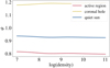 |
Fig. B.1. Value of ψ from Eq. (22) as a function of density for each typical EM from CHIANTI for the lines used in the 2LR method. The coefficients used to calculate ψ for every density value are defined by Eq. (24). |
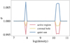 |
Fig. B.2. Value of ψ from Eq. (22) as a function of density for each typical EM from CHIANTI for the linear combinations of lines used in the LCR method. The coefficients used to calculate ψ for every density value are the result of the optimisation. For example, the coefficients used for every line at log(n) = 8.3 are the ones listed in Table 1. |
As we can see in Fig. B.1 (and consistent with the values of Table 3 at log n = 8.3), the 2LR method gives values of ψ that can be up to 20% above or below the target value of 1, leading to erroneous FIP bias determination. The ψ value for each EM depends somewhat on density as well. In contrast, the LCR method (Fig. B.2) yields ψ values that are less than 0.7% away from 1 at all densities, leading to much more accurate FIP bias determination than with the 2LR method.
We then trace ψ in Fig. B.3 using only the coefficients computed for the LCR method at a fixed density of log n = 8.3 and the contribution functions evaluated at different density values. We do so to determine the error one would commit by assuming a constant density of log n = 8.3 when determining the optimised coefficients (listed in Table 1) instead of using the density-dependent approach. In this case, ψ remains within 20% of the target value of 1 from below log n = 7 to log n = 9, meaning that the LCR method can perform as well as or better than the 2LR method in a significant range of densities, even when not taking the density dependence of the optimal coefficients into account. However, ψ deviates strongly from 1 for higher densities, up to a factor two if log n = 11 instead of 8.3.
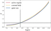 |
Fig. B.3. Value of ψ from Eq. (22) as a function of density for each typical EM from CHIANTI for the linear combinations of lines used in the LCR method. This time we use the coefficients listed in Table 1 computed at a fixed density of log n = 8.3 and the contribution functions are evaluated at the different density values. The dashed lines correspond to the density value assumed for the optimisation, and to the target value of ψ. |
All Tables
First ionization potential of the elements used for the tests, their coronal and photospheric abundances taken from Schmelz et al. (2012) and Grevesse et al. (2007), and the corresponding abundance bias relative to sulfur.
All Figures
|
Fig. 1. Top panel: composite map of the solar corona on June 3, 2012, in the 171 Å (red), 193 Å (green), and 211 Å (blue) channels of the AIA instrument aboard SDO. The black and red squares correspond to the regions of interest used for testing the method, and are centred on an AR and a CH, respectively. Middle panel: zoom on the AR region of interest (black square in top panel). Bottom panel: zoom on the CH region of interest (red square in top panel). |
| In the text | |
|
Fig. 2. Histogram of the EM(T) values in the first region of interest (black square) of Fig. 1. The colour scale and the size of the points correspond to the number of pixels containing an EM of a given value at a given temperature. We have also traced in full lines the typical EMs from CHIANTI that we use to optimise the cost function (Eq. (21)). The red line corresponds to an active region, the blue line to the quiet Sun and the yellow line to a coronal hole. |
| In the text | |
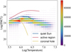 |
Fig. 3. Same as Fig. 2 but for the second region of interest (red square) of Fig. 1. |
| In the text | |
|
Fig. 4. Top: normalized contribution functions of the lines used for the 2LR method. Bottom: contribution functions of the lines used for the LCR method. All the contribution functions were calculated assuming a constant density of 108.3 cm−3. |
| In the text | |
|
Fig. 5. Results of FIP bias determination using the 2LR (left) and LCR (right) methods on the synthetic radiances in the first region of interest (black square) of Fig. 1: relative FIP maps (top) and their corresponding histograms (bottom), with matching colour scales. The DEM inversion code was not able to find a satisfactory solution in the pixels depicted in white. The vertical lines in the histograms correspond to the imposed uniform values of the relative FIP bias (for each of the low-FIP elements; see Table 2) that should ideally be retrieved. |
| In the text | |
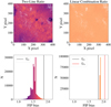 |
Fig. 6. Same as Fig. 5 but for the second region of interest (red square) of Fig. 1. |
| In the text | |
|
Fig. 7. Products between the EM and the contribution functions (𝒞LF, solid lines, and 𝒞HF, dashed lines), as functions of the temperature for both methods, using the coefficients in Table 1. Different colours correspond to different EMs from CHIANTI. |
| In the text | |
|
Fig. 8. Contributions of the different spectroscopic lines to the 𝒞LF(T) EM(T) product as a function of temperature for the CHIANTI AR EM. The total (dotted line) corresponds to the full red line in the bottom panel of Fig. 7. Here, Fe and Si line contributions are shown in ocher-red and blue-green colours, respectively. We separate the positive and negative contributions to the total. |
| In the text | |
|
Fig. 9. Map of the logarithm of the density in cm−3 obtained for the observation on October 17, 2007, from EIS spectra. We used the Fe XIII λ 202.02 and 203.83 line pair to calculate this density map. In the white pixels, fitting of the EIS lines failed. The density value of each pixel allows us to compute the optimal linear combination of lines to be used to determine the FIP bias in those pixels. |
| In the text | |
|
Fig. 10. First ionization potential bias maps obtained with different methods and the corresponding histograms. Left panel: FIP bias map obtained following DEM inversion (adapted from Baker et al. 2013). Right panel: FIP bias map obtained using the LCR method. In the white pixels, the fitting of the EIS lines we performed failed. In both FIP bias maps we only plot the pixels where our fitting was successful. |
| In the text | |
|
Fig. 11. Two-dimensional histogram of the FIP bias values of Baker et al. (2013) and those obtained using the LCR method. The white line is the first bisector, where both values are equal. |
| In the text | |
|
Fig. B.1. Value of ψ from Eq. (22) as a function of density for each typical EM from CHIANTI for the lines used in the 2LR method. The coefficients used to calculate ψ for every density value are defined by Eq. (24). |
| In the text | |
|
Fig. B.2. Value of ψ from Eq. (22) as a function of density for each typical EM from CHIANTI for the linear combinations of lines used in the LCR method. The coefficients used to calculate ψ for every density value are the result of the optimisation. For example, the coefficients used for every line at log(n) = 8.3 are the ones listed in Table 1. |
| In the text | |
|
Fig. B.3. Value of ψ from Eq. (22) as a function of density for each typical EM from CHIANTI for the linear combinations of lines used in the LCR method. This time we use the coefficients listed in Table 1 computed at a fixed density of log n = 8.3 and the contribution functions are evaluated at the different density values. The dashed lines correspond to the density value assumed for the optimisation, and to the target value of ψ. |
| In the text | |
Current usage metrics show cumulative count of Article Views (full-text article views including HTML views, PDF and ePub downloads, according to the available data) and Abstracts Views on Vision4Press platform.
Data correspond to usage on the plateform after 2015. The current usage metrics is available 48-96 hours after online publication and is updated daily on week days.
Initial download of the metrics may take a while.