| Issue |
A&A
Volume 632, December 2019
The XXL Survey: third series
|
|
|---|---|---|
| Article Number | A54 | |
| Number of page(s) | 17 | |
| Section | Cosmology (including clusters of galaxies) | |
| DOI | https://doi.org/10.1051/0004-6361/201628521 | |
| Published online | 27 November 2019 | |
The XXL Survey
XXXVIII. Scatter and correlations of X-ray proxies in the bright XXL cluster sample⋆
1
INAF – Osservatorio di Astrofisica e Scienza dello Spazio di Bologna, Via Piero Gobetti 93/3, 40129 Bologna, Italy
e-mail: This email address is being protected from spambots. You need JavaScript enabled to view it.
2
INFN, Sezione di Bologna, Viale Berti Pichat 6/2, 40127 Bologna, Italy
3
Department of Astronomy, University of Geneva, ch. d’Ecogia 16, 1290 Versoix, Switzerland
4
Astronomy Centre, University of Sussex, Falmer, Brighton BN1 9QH, UK
5
H. H. Wills Physics Laboratory, University of Bristol, Tyndall Ave, Bristol BS8 1TL, UK
6
Argelander Institut für Astronomie, Universität Bonn, 53121 Bonn, Germany
7
AIM, CEA, CNRS, Université Paris-Saclay, Université Paris Diderot, Sorbonne Paris Cité, 91191 Gif-sur-Yvette, France
8
Institut de Physique Theorique, CEA, Saclay, 91191 Gif-sur-Yvette, France
Received:
15
March
2016
Accepted:
11
June
2019
Abstract
Context. Scaling relations between cluster properties embody the formation and evolution of cosmic structure. Intrinsic scatters and correlations between X-ray properties are determined from merger history, baryonic processes, and dynamical state.
Aims. We look for an unbiased measurement of the scatter covariance matrix among the three main X-ray observable quantities attainable in large X-ray surveys: temperature, luminosity, and gas mass. This also gives us the cluster property with the lowest conditional intrinsic scatter at fixed mass.
Methods. Intrinsic scatters and correlations can be measured under the assumption that the observable properties of the intra-cluster medium hosted in clusters are log-normally distributed around power-law scaling relations. The proposed method is self-consistent, based on minimal assumptions, and requires neither external calibration by weak lensing, or dynamical or hydrostatic masses, nor the knowledge of the mass completeness.
Results. We analysed the 100 brightest clusters detected in the XXL Survey and their X-ray properties measured within a fixed radius of 300 kpc. The gas mass is the less scattered proxy (∼8%). The temperature (∼20%) is intrinsically less scattered than the luminosity (∼30%), but it is measured with a larger observational uncertainty. We found some evidence that gas mass, temperature, and luminosity are positively correlated. Time evolutions are in agreement with the self-similar scenario, but the luminosity–temperature and the gas mass–temperature relations are steeper.
Conclusion. Positive correlations between X-ray properties can be determined by the dynamical state and the merger history of the halos. The slopes of the scaling relations are affected by radiative processes.
Key words: surveys / X-rays: galaxies: clusters
Based on observations obtained with XMM-Newton, an ESA science mission with instruments and contributions directly funded by ESA Member States and NASA. Based on observations made with ESO Telescopes at the La Silla and Paranal Observatories under programme ID 089.A-0666 and LP191.A-0268.
© ESO 2019
1. Introduction
The physics of baryons and dark matter can be assessed with scaling relations between cluster properties (Pratt et al. 2009; Arnaud et al. 2010; Giodini et al. 2013). Ongoing and upcoming large surveys are measuring a wealth of cluster properties, e.g. optical richness, X-ray luminosity, and Sunyaev–Zel’dovich (SZ) flux (Laureijs et al. 2011; Planck Collaboration XXIX 2014; Bleem et al. 2015; Pierre et al. 2016; Melchior et al. 2017; Maturi et al. 2019).
Gravity is the driving force in structure formation and evolution, and makes clusters self-similar with observable properties following power-law relations in halo mass (Kaiser 1986; Giodini et al. 2013; Ettori 2013). Deviations from the self-similar scheme are due to non-gravitational processes, such as feedback and non-thermal mechanisms, which can contribute significantly to the global energy budget (Maughan et al. 2012).
The scaling relations are scattered by underlying processes that can affect different cluster properties to different degrees (Stanek et al. 2010; Truong et al. 2018). Numerical simulations (Stanek et al. 2010; Fabjan et al. 2011; Angulo et al. 2012; Saro et al. 2013) and observational studies (Maughan 2007; Vikhlinin et al. 2009a) confirm that the properties are log-normally distributed. Broadly speaking, the scatter is related to the regularity of the clusters (Sereno & Ettori 2015a,b) and to deviations from equilibrium (Fabjan et al. 2011; Saro et al. 2013). Well-behaved proxies with small scatter can be used to provide accurate measurement of the mass of galaxy clusters, which is crucial in important branches of cosmology and astrophysics (Ettori et al. 2009; Vikhlinin et al. 2009b; Mantz et al. 2010; Planck Collaboration XX 2014).
If we measure scalings, scatters, and correlations of scaling relations, we can study the forces driving cluster formation and evolution. In this paper, we investigate X-ray properties measurable in large surveys. We propose a novel statistical method where intrinsic scatters are measured exploiting the expected linearity of the relations even without knowing the mass of the clusters. An observable property of a galaxy cluster can be a good proxy if it is easy to measure and is well behaved. Intrinsic scatter enables us to determine such a variable. We can view the proxy with the lowest intrinsic conditional scatter with respect to some basic cluster characteristic as optimal.
We exploit the XXL Survey, the largest completed XMM-Newton project (Pierre et al. 2016; hereafter XXL Paper I). Two sky regions for a total of 50 deg2 have been surveyed, and several hundred galaxy clusters out to redshift ∼2 have been detected (Adami et al. 2018; hereafter XXL Paper XX). We consider the three main X-ray global quantities measured by the mission, i.e. temperature, luminosity, and gas mass.
The paper is organised as follows. The regression method and its extension to multi-response variables are described in Sects. 2 and 3, respectively. The data sample is introduced in Sect. 4. Theoretical expectations are briefly discussed in Sect. 5. Section 6 presents the results. Section 7 is devoted to comparison with previous analyses. Final considerations are presented in Sect. 8. Appendix A presents a simple recipe to deal with asymmetric errors and logarithmic variables. Additional figures are presented in Appendix B.
The framework cosmological model in use in the XXL papers is the flat ΛCDM universe with density parameter ΩM = 0.28, and Hubble constant H0 = 70 km s−1 Mpc−1, as found from the study of the final nine years of cosmic microwave background observations of the Wilkinson Microwave Anisotropy Probe satellite (WMAP9), combined with baryon acoustic oscillation measurements and constraints on H0 from Cepheids and type Ia supernovae (Hinshaw et al. 2013). As usual, H(z) is the redshift dependent Hubble parameter and Ez ≡ H(z)/H0. When H0 is not specified, h is the Hubble constant in units of 100 km s−1 Mpc−1.
The parameter OΔ denotes a cluster property measured within the radius rΔ, which encloses a mean overdensity of Δ times the critical density at the cluster redshift, ρcr = 3H(z)2/(8πG).
“log” is the logarithm to base 10 and “ln” is the natural logarithm. Results for natural logarithm are quoted as percents, i.e. 100 times the dispersion in natural logarithm.
By intrinsic scatter we mean the standard deviation of the conditional probability, which is the probability of the temperature given the mass. If the conditional probability is related to the measurement process, i.e. the probability of the measured output given true input, we name it statistical measurement uncertainty. We do not give the name “scatter” to the standard deviation of the marginalised distribution (e.g. the distribution of temperatures). Throughout the paper, we denote the intrinsic scatter as σ and the measurement uncertainty as δ.
2. Regression scheme
In this section, we describe the Bayesian fitting procedure used to retrieve the scaling relations and the intrinsic scatter. We assume that the cluster properties (temperature, luminosity, gas mass) are power laws of some basic property (e.g. mass). Here we focus on the logarithms of these quantities, which are thus linearly related with each other.
In a nutshell, we first appoint a basic intrinsic cluster feature (denoted Z as the reasoning would apply to the mass as well as to other choices). For any measurable property (e.g. the temperature) we distinguish three variables, see Fig. 1: (i) XZ, the latent quantity that is exactly linked to Z through a functional relation X(Z) (Maughan 2014); (ii) X, the true quantity that would be measured in a theoretical observation with infinite accuracy and precision (Feigelson & Babu 2012). X is intrinsically scattered with respect to XZ; and (iii) x, the manifest result of the measurement process, which shows some observational noise with respect to X.
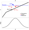 |
Fig. 1. Graphic view of some quantities playing in the Bayesian regression scheme, see Sect. 2: the measurement results (blue); the true property values (red); the rescaled values of a basic feature (black). |
Similarly to X, we can consider an additional cluster property Y and the related y and YZ. If the latent variables (XZ, YZ) are linearly related to Z, they are linearly related with each other. We can then identify the best proxy with the X-ray observable characterised by the lowest conditional intrinsic scatter with respect to Z. In this way, the optimal proxy can be established even if we do not know the cluster mass.
We still need the mass if we want to calibrate the scaling relations and unambiguously identify the best proxy as the best mass proxy. In principle, Z can be any fundamental property of the cluster. Since we do not measure the mass itself, our analysis is based on Z being the quantity that can best characterise the X-ray properties of the clusters and minimise the scatter. Even though on a theoretical basis the most suitable candidate for this role is the mass, it is not guaranteed that Z is the mass. It could be another quantity, for example the optical richness or the SZ signal, or one of the three X-ray properties measured in the present paper. However, this last hypothesis can be discarded if the estimated intrinsic scatter values are not null.
2.1. Scaling and distributions
In order to quantify the intrinsic scatter of the X-ray properties, we follow the regression scheme detailed in the series Comparing Masses in Literature (CoMaLit, Sereno & Ettori 2015a,b, 2017; Sereno et al. 2015) and in Sereno (2016). This scheme accounts for time evolution, correlated intrinsic scatter, and selection effects (Malmquist/Eddington biases). In this section we consider a pair of observables. In the next section, we generalise the procedure to the case of multiple response variables.
As a result of the measurement of the jth cluster, the observable xj, yj, and the related uncertainty covariance matrix Vδ, j are known. On the other hand, {XZ, j, YZ, j}, {Xj, Yj}, and the covariance matrix of the intrinsic scatters Vσ, j are unknowns to be determined under the assumption of linearity.
In case of a linear relation, XZ and YZ are related to the same covariate variable Z as
 (1)
(1)
 (2)
(2)
where α denotes the normalisation, the slope β accounts for the dependence with Z and the slope γ accounts for the redshift-evolution, and Fz is the re-normalised Hubble parameter: Fz = Ez/Ez(zref). Here and in the following, we assume a power-law dependence on Fz for the redshift-evolution of the observables.
The relations between Z, XZ, and YZ are deterministic and they are not affected by scatter. We assume that the uncertainty on the spectroscopic redshift z is negligible.
If we do not know the value of Z, the two slopes and the two normalisations in Eqs. (1) and (2) are redundant. We then assume that X is an unbiased proxy of Z, i.e. we fix αX|Z = 0, βX|Z = 1, and γX|Z = 0. Fixing the parameters of the X − Z relation rather than Y − Z is just a matter of rescaling, which does not affect the analysis of the intrinsic scatter. In the absence of a direct measurement of Z, any bias between X and Z (i.e. αX|Z ≠ 0) is degenerate with the estimated overall normalisation of the scaling between Y and Z. The data analysis can only constrain the relative bias between X and Y (Sereno & Ettori 2015b; hereafter CoMaLit-I).
The measured and the true values of the quantities are related as
 (3)
(3)
where  is the bivariate Gaussian distribution;
  is the uniform distribution; Vδ, j is the uncertainty covariance matrix whose diagonal elements are denoted
  and
and  , and whose off-diagonal elements are denoted ρxy, jδx, jδy, j. The proportionality symbol in Eq. (3) indicates that the function on the right-hand side is not normalised.
The probability distribution in Eq. (3) is truncated for yj < yth, j, which accounts for selection effects when only clusters above an observational threshold (in the response variable) are included in the sample, i.e. the Malmquist bias (Sereno et al. 2015; hereafter CoMaLit-II).
To shorten the notation in Eq. (3) and similarly in the following, we drop the explicit dependence on the fixed parameters, i.e. Vδ, j and yth, j, on the left-hand side. On the right-hand side we do not express the functional dependence on the random variables xj and yj.
The observational threshold yth may not be exactly known. This is the case when the quantity which the selection procedure is based on differs from the quantity used in the regression. As an example, XXL clusters are selected according to their flux within 1′, whereas we consider the luminosity within 0.3 Mpc in the regression (see Sect. 4). We have then to consider the additional relation
 (4)
(4)
where δyth, j is the uncertainty associated with the measured threshold yth, obs, j. This saves us from adding new quantities (e.g. the observed flux) to the regression scheme.
We assume that the intrinsic scatter values are Gaussian. It is
 (5)
(5)
where Vσ, j is the scatter covariance matrix whose diagonal elements are denoted  and
and  , and whose off-diagonal elements are denoted ρXY|Z, jσX|Z, jσY|Z, j, and Yth, j is the threshold in the response variable,
 (6)
(6)
Even though the selection procedure is based only on the value of the measured y rather than the value of Y, any threshold in y affects all the probability distributions. We do not sample a generic distribution of clusters, but we select them and we have to model the distribution of the sampled objects. Hence, the distribution of Y given Z for a generic cluster from the full population differs from the distribution specific to a selected sample, which follows Eq. (5) and it is truncated.
We assume that the intrinsic scatters are time-dependent, hence the subscript j in the covariance matrix, but do not depend on Z (Rozo et al. 2010). The time evolution of the intrinsic scatter and of the correlation can be modelled as
 (7)
(7)
 (8)
(8)
 (9)
(9)
The intrinsic distribution of Z can be approximated with a mixture of Gaussian functions (Kelly 2007; CoMaLit-II; Sereno & Ettori 2015a; CoMaLit-IV). In the simplest but still effective case of one component (Sereno 2016),
 (10)
(10)
Most of the parent populations of astronomical quantities (e.g. the halo mass function or the luminosity function) are locally exponential (in log-space), i.e. Pparent(Z) ∼ exp(−aZ). However, here we have to model just the distribution of the clusters included in the sample rather than the full population. Once the parent population is filtered by the selection process, a Gaussian distribution provides a reliable approximation (CoMaLit-IV).
The redshift evolution of the mean of the Z-distribution can be modelled as (CoMaLit-IV),
 (11)
(11)
where μZ, 0 is the local mean and Dz is the luminosity distance. We renormalise the distances such that Dz(zref) = 1.
The dispersion of the Z-distribution evolves as
 (12)
(12)
The dependence on Fz is enough to account for the redshift evolution of the scaling relations (see Eqs. (1) and (2)) and of the scatter (see Eqs. (7)–(9) and Eq. (12)). This is justified by theoretical predictions based on the self-similar model, by results of numerical simulations, and by observational fits (CoMaLit-IV). On the other hand, we introduce an explicit dependence on the cosmological distance for the evolution of the covariate distribution, see Eq. (11). The completeness of a sample selected according to either flux or signal-to-noise ratio depends on the distance (CoMaLit-IV). The redshift dependence in Eq. (11) is general enough to address even more complicated cases.
2.2. Priors
Priors have to be conveniently non-informative (CoMaLit-I; CoMaLit-II). The priors on the intercept αY|Z and on the mean μZ, 0 are flat,
 (13)
(13)
where ϵ is a small number. In our calculation, ϵ = 10−4. The prior on the correlation ρXY|Z, 0 is flat too:
 (14)
(14)
We model the prior probability of the slopes and of the time evolution as a Student’s t1 distribution with one degree of freedom,
 (15)
(15)
This is equivalent to uniformly distributed direction angles arctanβ and arctanγ.
As non-informative priors for the evolution of scatter and correlations, we consider uniform distributions. Since intrinsic scatters are expected to slightly increase with redshifts (CoMaLit-IV), we assume
 (16)
(16)
and
 (17)
(17)
For the evolution of the dispersion of the Z-distribution we adopt
 (18)
(18)
For the precision, i.e. the inverse of the variance, we adopt a nearly scale-invariant gamma distribution,
 (19)
(19)
where the rate r and the shape parameter λ are fixed to r = λ = ϵ so that the prior spans a considerable range and is nearly constant in logarithmic bins.
Alternatively to non-informative priors, we consider strong assumptions. The evolution of scatter and correlations is poorly constrained in samples of ∼100 objects (Sereno 2016). In our reference regression scheme, we only constrain the redshift weighted scatter and we fix
 (20)
(20)
3. Multi-response regression scheme
The scheme detailed in Sect. 2 can be generalised to the simultaneous regression of n(≥2) observables. In this scheme, yij is the jth measurement of the ith observable, Yij is the true value, and YZ, ij is the latent unscattered quantity which fits the scaling relation. To simplify the notation, in the following we dismiss the subscripts for the time dependence of the scatter. The scaling relation of the ith property is expressed as
 (21)
(21)
Due to degeneracy, we anchor the scaling parameters of the first response variable, i.e. αY1|Z = 0, βY1|Z = 1, and γY1|Z = 0. The reference Z variable is modelled as in Eq. (10). In the absence of Malmquist biases, Z is the expected value of Y1 given Z, ⟨Y1|Z⟩ = Z.
The intrinsic scatters shape the distribution of the true quantities around the model predictions. For the jth cluster
 (22)
(22)
where  is the multivariate Gaussian distribution, Vσ is the n × n scatter covariance matrix whose diagonal elements are the intrinsic variances
  and whose off-diagonal elements can be expressed in terms of the correlations as ρYaYb|ZσYa|ZσYb|Z. The threshold for the jth measurement of the ith response variable is Yth, ij.
The measured and the true values are related as
 (23)
(23)
where Vδ, j is the n × n uncertainty covariance matrix of the jth cluster. The thresholds for the measured and the true response values are related as
 (24)
(24)
and
 (25)
(25)
where yth, obs,ij is the observational threshold, δyth, ij is the related uncertainty, and δy, ij is the uncertainty associated with yij.
As we mention in Sect. 2, the Malmquist bias is treated with the inclusion of the smooth truncations in Eqs. (22) and (23).
3.1. Priors
We express the prior on the inverse of the intrinsic scatter matrix in terms of the Wishart distribution,
 (26)
(26)
where d is the number of degrees of freedom and S in the n × n scale matrix. We take d = n + 1, so that the marginalised prior distribution of the correlation factors is uniform between −1 and 1. In analogy to the variances in Eq. (19), we model S as a scalar matrix with diagonal elements
 (27)
(27)
The Wishart prior is widely regarded as non-informative, even though it favours high variance in the case of high correlation. Other priors are defined as in Sect. 2.2.
4. Sample
The XXL survey covers a total area of ∼50 deg2 with an X-ray sensitivity of ∼10−14 erg cm−2 s−1 in the [0.5–2] keV band for extended sources (Pacaud et al. 2016; hereafter XXL Paper II). The survey has uncovered more than 300 galaxy clusters out to redshift ∼2 (XXL Paper XX) over a wide range of nearly two decades in mass (Lieu et al. 2016; hereafter XXL Paper IV). The XXL programme has the potential to constrain cluster scaling relations and cosmological parameters at the same time (Pacaud et al. 2018; hereafter XXL Paper XXV).
We consider here the sample of the 100 brightest clusters (XXL-100-GC) from the first data release (DR1, XXL Paper I). The candidate clusters were selected by setting a lower limit of 3 × 10⁻¹⁴ erg cm−2 s−1 on the source flux in the soft X-ray band within a 1′ aperture (XXL Paper II). We analyse the spectroscopic temperature within 300 kpc, T300 kpc, the luminosity in the rest-frame soft band [0.5–2.0] keV within 300 kpc,  (Giles et al. 2016; hereafter XXL Paper III), and the gas mass. Here, we consider the gas mass in a sphere of radius equal to 300 kpc, Mgas, 300 kpc, which is computed following the procedure described in Eckert et al. (2016; hereafter XXL Paper XIII), which we refer to for details. The full set of measurements is available for 96 clusters. The sample has a mean redshift of z = 0.38 with standard deviation of Δz = 0.24. The sample covers an extended range in temperature, from small groups at T300 kpc ≲ 1 keV to rich clusters at T300 kpc ≲ 7 keV, even though the most massive and rare clusters from the extreme tail of the cosmological halo mass function are absent due to the limited survey area coverage. For a comprehensive discussion of the sample properties we refer to XXL Paper II.
In the following, we recover the intrinsic scatters and correlations of the X-ray properties without having access to the mass. We use a simplified notation in the log-space. The measured gas mass, temperature, and luminosity in logarithmic units are
 (28)
(28)
 (29)
(29)
 (30)
(30)
For the latent variables, we cannot strictly follow the convention in Sects. 2 and 3, since X-ray observables in linear space are usually indicated by capital letters (e.g. Mgas, 300 kpc). Then, if mg is the measured gas mass (y), the hypothetical measurement in the absence of noise (Y) is  and the unscattered gas mass (YZ) is
  . The same convention applies to temperature and luminosity.
For our analysis, we follow a data-driven approach and we consider as proxies only X-ray properties measured within fixed physical radii. The use of quantities measured in a given overdensity radius as proxy can be ambiguous to some degree. If we know the overdensity radius, by definition we know the mass too. Let OΔ be a generic observable quantity (e.g. temperature or richness) within the overdensity radius rΔ. In practice, we use only a part (rΔ) of the full information we already have (the mass MΔ) to get a deteriorated version, i.e. the mass proxy MΔ(OΔ) calculated through the scattered scaling relation applied to OΔ, of the main information itself (the mass MΔ). In this sense we lose information. This can be corrected with iterative approaches by determining rΔ, OΔ, and MΔ at the same time. However, we still have to rely on very strong priors (usually the knowledge of how rΔ scales with some observable property). This has little effect if the observable is poorly correlated with the radius (e.g. the X-ray luminosity emitted from a very large area), but it is a major problem otherwise (e.g. the gas mass). Valuable mass proxies can be highly correlated with the integration radius.
The use of X-ray properties measured within fixed physical radii also minimise the impact of the assumed cosmological parameters on our results (Sereno & Ettori 2015b). A different frame-work cosmology would mostly imply a different normalisation and a slightly different time-dependence of the relations. Slopes and scatters would be minimally affected. At present, analyses of number counts (XXL Paper XXV) and clustering (Marulli et al. 2018; hereafter XXL Paper XVI) of XXL clusters are compatible with our reference cosmological model.
4.1. Covariance uncertainty matrix
The knowledge of the covariance uncertainty matrix is crucial in order to obtain unbiased estimates of the intrinsic scatters and of their correlations. Measurements of luminosity and temperature are based on the spectroscopic analysis of the core region and are largely independent of the gas mass measurement process, which exploits the photometry and the surface brightness profile in annular regions. However, the photons are the same and the gas mass measurement process uses the estimated temperature to convert the observed surface-brightness profiles into emission-measure profiles. This conversion is largely insensitive to the temperature and metallicity as long as the temperature exceeds ∼1.5 keV. In most cases the temperature and the gas measurement are nearly uncorrelated.
To estimate the uncertainty covariance matrix we proceed in the following way. Luminosity and temperature are estimated in a single measurement process. Their correlation is an output of the spectroscopic analysis. We approximate the probability distribution of the observed luminosity and temperature as a bivariate Gaussian.
Measured temperature and gas mass are correlated too. The estimate of the gas mass relies on the conversion of the observed surface brightness into the emission measure. The conversion factor is computed using T300 kpc and simulating a single-temperature absorbed thin-plasma model with the APEC code (XXL Paper XIII).
To estimate the full covariance uncertainty matrix, we extract 105 couples of luminosity and temperature for each cluster from the approximated bivariate normal distribution. We then compute the new conversion factor from surface brightness into emission measure for the sampled temperature and we compute the corresponding gas mass by rescaling. We finally extract a new gas mass measurement from a normal distribution centred on the rescaled Mgas, 300 kpc and with standard deviation equal to the observational uncertainty δMgas, 300 kpc. The final correlation matrix is computed from the sampled values of temperature, luminosity, and gas mass.
4.2. Selection effects
Cosmological studies of number counts and abundance evolution require a very detailed study of the completeness. Observed properties have to be related to the underlying mass function, and the selection function can be expressed in terms of the true cluster parameters rather than in terms of their measured counterparts affected by measurement errors.
The selection and validation of the XXL-100-GC sample is described in XXL Paper II. Here we just recall the main features relevant for our analysis. The XXL-100-GC sample was chosen with a flux-limit selection in a fixed angular aperture. The flux limit of the final catalogue is 3 × 10⁻¹⁴ erg s−1 cm−2 in the [0.5–2.0] keV band within a 1′ radius aperture. Assuming temperature equal 3 keV, metallicity equal to 0.3, and redshift z = 0.3, this is equivalent to a total MOS1+MOS2+PN count rate of 0.0332 cts s−1 in [0.5–2] keV.
The C1+2 pipeline selection function of the XXL Survey depends on cluster profile, emissivity, and position (XXL Paper II). The dependence on the exposure and background level is encapsulated in the pointing under consideration, and the off-axis angle is implicitly given by the sky position (XXL Paper II). Candidate clusters are then confirmed by visual inspection.
When we express the selection function in terms of the true intrinsic parameters, we have to consider that a cluster with a given true count rate can exceed the cut or fail depending on the flux measurement errors, which depend on the local exposure time and therefore on the pointing on which the source was detected. Finally, in regions where several pointings overlap, the completeness must follow exactly the order and manner in which the two selection steps are applied to the source candidates.
The full information of the selection function and of the completeness of the sample is needed in cosmological studies; instead, simpler methods are better suited to studies focused on the scaling relations. The CoMaLit approach can be applied to heterogeneous samples too. If we do not aim to express the observed distribution of clusters in terms of the underlying mass function, we have to just properly model the distribution to avoid Eddington and Malmquist biases. The distribution has to be flexible enough to fit the data.
Within this framework, the Malmquist bias and the probability of exceeding a given count rate can be simply modelled in terms of the observed flux as a step function rather than as a more complicated position dependent probability of the true flux.
The correction for the Malmquist bias is relevant in the case of the X-ray luminosity as a response variable. The flux limit is set within a 1′ aperture. We compute the luminosity threshold extrapolated out to 300 kpc at the cluster redshift, by assuming a β-profile with core radius rc = 0.15 r500 and β = 2/3 (XXL Paper III). This procedure gives the luminosity threshold  for each cluster. According to the notation of Sects. 2 and 4, the threshold for the jth cluster is
 (31)
(31)
The uncertainty δyth, j related to the extrapolation procedure is estimated by considering a range of radial profiles with scatter in slope of σβ ∼ 0.1, scatter in core radius of σ(rc/r500)∼0.1, and correlation ρβrc ∼ 0.66 as representative of the sample of the 45 bright nearby galaxy clusters in Mohr et al. (1999). The median δyth is ∼3%, but the distribution of values shows a long tail at larger values, so that the mean is ∼6% and the standard deviation is ∼7%.
5. Theoretical predictions
The self-similar scenario of cluster formation and evolution was first proposed by Kaiser (1986) and later on extended and integrated (see e.g. Giodini et al. 2013). If gravity is the driving force of structure formation, X-ray quantities follow power laws.
The relations for quantities within a fixed physical length differ from the canonical ones within the overdensity radius. Here the reference radius R is constant and does not scale with the mass. On the other hand, the density within R is not constant and changes with the mass. Since the density is not a constant multiple of the critical density the time dependence factor  connected to the critical density does not enter the relations.
Under the assumptions that clusters are closed boxes and baryons track the total mass,
 (32)
(32)
If the cluster is near hydrostatic equilibrium, then
 (33)
(33)
Finally, the X-ray emission in the soft band scales as
 (34)
(34)
with no appreciable temperature dependence (Ettori 2015). By definition, luminosity can be written as
 (35)
(35)
By rearranging Eqs. (32)–(35), we obtain the self-similar scaling relations for properties measured within fixed radii,
 (36)
(36)
 (37)
(37)
 (38)
(38)
Reported slopes involving the luminosity are appropriate for the soft band (Ettori 2015).
Baryonic processes can disrupt the self-similar relations. Active galactic nucleus (AGN) feedback or radiative cooling can remove cold, dense gas from the inner regions of low-mass clusters, which makes the gas mass versus total mass and luminosity versus total mass relations steeper and the temperature-mass relation shallower (Truong et al. 2018).
Scaling relations can be scattered by a number of processes acting in different directions. Non-thermal sources of gas pressure, temperature inhomogeneity, substructures and clumps, unvirialised bulk motions, and subsonic turbulence play a role (Battaglia et al. 2012; Rasia et al. 2012).
Triaxiality is an additional source of scatter (Limousin et al. 2013; Sereno et al. 2013). Observed signals depend on the orientation of the cluster (Gavazzi 2005; Oguri et al. 2005; Sereno 2007; Sereno & Umetsu 2011; Limousin et al. 2013; Sereno et al. 2013). For systems whose major axis points toward the observer, which are typically over-represented in signal-limited samples, X-ray luminosities and gas mass derived under the standard assumption of spherical symmetry are overestimated. On the other hand, the majority of randomly oriented clusters are elongated in the plane of the sky and properties can be underestimated.
A certain degree of correlation between intrinsic scatters is in place and has to be considered in multi-property galaxy cluster statistics to properly model the scaling relations (Evrard et al. 2014; Rozo et al. 2014; Maughan 2014; Mantz et al. 2015). Correlations can come from internal structure, formation history, orientation, environment, and uncorrelated structure (Angulo et al. 2012).
The X-ray luminosity depends on the assembling history of the clusters (Mantz et al. 2016a). Massive mergers impact the luminosity-mass relation (Torri et al. 2004). The dynamical state of the cluster can cause a positive correlation between luminosity and temperature (Mantz et al. 2016b). Apart from transient shocks, luminosity and temperature can be depressed in merging clusters where energy in bulk motions has not yet virialised. On the other hand, dynamically relaxed, hot clusters show bright cores with higher than average luminosities and approximately average temperatures. Perturbed or relaxed clusters move coherently along the luminosity–temperature relation (Rowley et al. 2004; Hartley et al. 2008).
Intracluster medium (ICM) processes impact correlations too. Radiative cooling reduce the amount of gas in the smallest systems, and at the same time their total luminosity (Truong et al. 2018).
Ettori (2015) showed how the normalisations of the scaling relations between the hydrostatic mass and the gas mass, the gas temperature, the X-ray bolometric luminosity, and the integrated Compton parameter depend upon the gas density clumpiness, the gas mass fraction, and the logarithmic slope of the thermal pressure profile. Scatter in the thermal pressure profile can cause a positive correlation between the spectroscopic estimate of the temperature and the X-ray luminosity. Clumpiness induces positive correlation between the luminosity and the gas mass estimated under the hypothesis of a smooth distribution. Ettori (2015) also argued that deviations of the observed slopes from the self-similar expectations can be explained with a mass dependence of the gas mass fraction and of the logarithmic slope of the thermal pressure profile.
X-ray quantities in numerical simulations are positively correlated (Stanek et al. 2010; Truong et al. 2018). Stanek et al. (2010) performed a numerical study of the intrinsic covariance of cluster observables using the Millennium Gas Simulations. They adopted two different physical treatments: shock heating driven by gravity only (GO), or cooling and preheating (PH). The results in Stanek et al. (2010) depend on the adopted scheme. They found correlation factors at redshift zero between bolometric luminosity, spectroscopic-like temperature, and gas mass within r500 of ρlt|m = 0.67 (0.73), ρlmg|m = 0.60 (0.76), ρmgt|m = 0.42 (0.37) for the GO (PH) simulation.
6. Results
As reference analysis, we consider the statistical approach detailed in Sect. 2 in which X-ray observables are analysed in pairs. Since the procedure is symmetric and both X and Y are affected by scatter, the results do not change whether we associate one observable with either X or Y. The analysis was performed with the R-package LIRA1. As reference redshift, we consider zref = 0.01. Results for the scaling parameters and the intrinsic scatter are summarised in Table 1.
Observed scaling relations.
As an alternative method, we fitted the three X-ray observables at once (see Sect. 3). The Bayesian hierarchical multi-response model was sampled with JAGS2.
A critical aspect in Bayesian data analysis is the computational efficiency of the sampling of the posterior probability distribution. Gibbs sampling or other methods can efficiently constrain the distribution (Kelly 2007; Mantz 2016), but problems may arise for non-standard distributions. This is the case of the truncated multi-normal distributions presented in Sect. 3. To circumvent the problem, we neglect the truncation in Eq. (22), but we still consider the truncation in Eq. (23), which is much easier to sample since the uncertainty covariance matrix is known and fixed. We tested that this approximate scheme can still correct for the main effects of the Malmquist bias.
In our multi-response analysis, the gas mass acts as the Y1 variable. As for the analysis in pairs, the choice of the Y1 variable does not affect the measurement of the scatter. Results are summarised in Table 2. The agreement between the two alternative regression methods is substantial. Values listed in Tables 1 and 2 are in base 10 logarithm.
6.1. Scaling
Results of the reference regression analysis are reported in Table 1. Measured gas mass, temperature, and luminosity are aligned quite well, see Fig. 2. The marginalised 2D posterior probabilities are given in Appendix B.
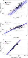 |
Fig. 2. Scaling relations. The black points indicate the data, the blue lines represent the fitted scaling relation at the median redshift. The dashed blue lines show the median scaling relation (solid blue line) plus or minus the intrinsic scatter σY|Z. The shaded blue region encloses the 68.3% confidence region around the median due to uncertainties on the scaling parameters. The red line shows the self-similar prediction. Top panel: scaling between luminosity and temperature: l − t. Middle panel: scaling between gas mass and temperature: mg − t. Bottom panel: scaling between luminosity and gas mass: l − mg. |
The l − t and mg − t relations are steeper than the self-similar predictions. This is confirmed by the multi-response analysis (see Table 2). There is no statistical evidence for time evolution, i.e. the γ parameters are consistent with zero. Parameter degeneracies can be analysed with the 2D probability functions. As is well known, slope and intercept are anti-correlated (see top left panels in Figs. B.1–B.3).
Measured slopes are consistent with a prominent role of radiative cooling and AGN feedback in low-mass systems (see Sect. 5). Stellar formation consumes the reservoirs of cold gas in the inner regions. Even though AGN feedback balances against excessive cooling, it expels gas from the cluster core, which also reduces the luminosity and the total gas supply. As a result of these baryonic processes, which are most effective in low-mass systems, the l − t and mg − t relations are steeper than the self-similar predictions, in agreement with our results.
6.2. Intrinsic scatter
The gas mass is the least scattered proxy,  (8.2 ± 3.0%), followed by temperature, ⟨σt(Y)|Z⟩=0.09 ± 0.02 (21.5 ± 4.2%), and luminosity, ⟨σl(Y)|Z⟩=0.19 ± 0.08 (43.6 ± 18.5%) (see Fig. 3). In the reference analysis, the three X-ray quantities were analysed in pairs, and we have two measurements of each scatter. The scatter values quoted above are obtained as the weighted mean and the standard deviation of the probability density obtained by combining the results from the two regressions summarised in Table 1.
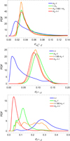 |
Fig. 3. Inferred probability density functions of the conditional intrinsic scatter with respect to the mass substitute. The blue and the green lines show the results based on the fits of pairs; the orange and the red lines show the densities obtained with the joint analysis of pair fits and with the multi-response regression, respectively. Top panel: gas mass intrinsic scatter. Middle panel: temperature intrinsic scatter. Bottom panel: luminosity intrinsic scatter. |
The reference results (orange lines in Fig. 3) are fully consistent with the results from the multi-response analysis (red lines in Fig. 3), when we obtain  ,
,  and
and  . Due to skewness, the mean and standard deviation slightly differ from the biweight estimators quoted in Table 2.
The probability distribution of the luminosity intrinsic scatter extends over a significantly wider range than gas mass and temperature with a tail at the upper end (see Fig. 3). The standard deviation, i.e. the quoted uncertainty, is then larger than for mg and t. Furthermore, the analysis of luminosity is more directly affected by Malmquist bias, which we treat as a threshold in the observed luminosity (see Sect. 4.1). Thresholds are expressed in terms of probability distributions (see Eqs. (4), (6), (24), (25)), which affects the precision within which regression parameters are recovered.
The intrinsic scatter is best constrained when at least one low-scatter proxy (e.g. the gas mass) is included in the fitting procedure. As seen from the comparison with the multivariate analysis in the middle and lower panels of Fig. 3, the l − t fitting overestimates the larger scatter, i.e.  , and underestimates the smaller scatter, i.e.
  . These two scatters are in fact anti-correlated (see Fig. B.1). The posterior probability distributions are compatible, however.
The temperature is intrinsically less scattered than the luminosity, but is measured with a larger uncertainty. The two effects partially counter-balance and make the two proxies nearly as effective.
The time evolution of scatter is not well constrained. Parameter values are affected by large statistical uncertainties and are consistent with zero.
Our estimates of the scatter can be slightly overestimated since we compare deprojected quantities measured within the sphere (e.g. the gas mass) to projected quantities measured within the cylinder (e.g. the temperature and the luminosity). The dispersion associated with the non-universality of the density profiles slightly inflates the measured scatter.
In our analysis, we assume that the variable X is an unbiased proxy, i.e. Eq. (1) reduces to XZ = Z. The role of X was covered by either the temperature or the gas mass. The gas mass also works as Y1, i.e. the analogue of X in the multi-response analysis. These assumptions are in line with our expectations for quantities measured within a fixed radius, when Mg ∝ M and T ∝ M (see Sect. 6.1). However, the determination of the conditional scatter and of the correlation factors is independent of the assumption on X. The estimates of scatter and slope are just weakly correlated (see Figs. B.1–B.3 and CoMaLit-IV). We further validate the stability of our results by considering tilted relations between X and Z (e.g. XZ = 3 × Z) or interchanging the roles of Y and X. Notwithstanding the different values of βX|Z, the results for scatter covariance matrix are the same.
6.3. Scatter correlations
Our analysis suggests that the intrinsic scatter of gas mass, temperature, and luminosity are positively correlated, i.e. clusters of a given mass that are more luminous than average have high temperature and an excess of gas mass. The probability distributions are peaked towards ρXY|Z ∼ 1. Strong correlations are slightly preferred, but the evidence is marginal due to the large statistical uncertainties. In fact, positive correlation is inferred at just the 1σ confidence level. Lower values of the correlation cannot be excluded (see the last rows of Figs. B.1–B.3). This is confirmed by the multi-response analysis (see Fig. B.4).
The intrinsic correlation ρXY|Z is partially degenerate with the slope of the relation βY|Z (see Figs. B.1–B.3).
Positive correlation between the properties of the ICM is expected as a result of formation history and dynamical state (see Sect. 5). Dynamically relaxed clusters are usually hotter and more luminous than merging systems of comparable total mass where the ICM has yet to virialise (Rowley et al. 2004; Hartley et al. 2008; Mantz et al. 2016b). Positive correlation between the luminosity and the gas mass estimated under the hypothesis of a smooth distribution can be induced by clumpiness and the degree of regularity of the system (Ettori 2015). Luminosity and gas mass can be overestimated in triaxial clusters elongated along the line of sight.
Our results support positive correlations even though the large statistical uncertainties (δρ ∼ 0.5; see Table 2) prevent us from distinguishing between extreme scenarios (ρ ≲ 1) and mild effects of co-evolution (ρ ≳ 0).
6.4. Distribution of the selected clusters
As expected for flux-limited selected samples, we find that the distributions of gas mass and temperature evolve with redshift, with more massive clusters preferentially included at high redshifts, see Table 3 and Fig. 4. These distributions are found as a result of the regression procedure, which does not exploit the knowledge of the mass completeness function obtained by numerical simulations, see Sect. 4.2, but recovers the distributions from the data.
Intrinsic distributions of the observed samples modelled as Gaussian functions.
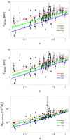 |
Fig. 4. Time dependence of the X-ray observables of the selected clusters. Measured values are shown as a function of redshift (black points). The full lines plot the value of the unscattered observable below which a given fraction of the selected sample is contained. From top to bottom, the red, green, and blue lines show the 85%, 50%, and 15% levels (μZ), respectively. The shaded green region encloses the 68.3% confidence region around μZ(z) due to uncertainties on the parameters. Top panel: time dependence of the temperatures as inferred from the l − t relation. Temperatures are in units of keV. Middle panel: time dependence of the distribution of temperatures of the selected clusters as inferred from the mg − t relation. Bottom panel: time dependence of the distribution of gas masses of the selected clusters as inferred from the l − mg relation. Masses are in units of 1014 M⊙. |
The Gaussian function provides a good approximation to the redshift evolving distributions (see Figs. 5–7). The temperature distributions derived from the analysis of the l − t and of the mg − t are fully consistent.
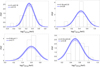 |
Fig. 5. Temperature function of the clusters from the l − t analysis in four redshift bins. The black histogram groups the observed temperatures. The blue line is the normal approximation estimated from the regression at the median redshift in the bin. The shaded blue region encloses the 68.3% probability region around the median relation due to uncertainties on the parameters. The function for the observed temperatures is estimated from the regression output, i.e. the function of the unscattered temperatures, by smoothing the prediction with a Gaussian whose variance is given by the quadratic sum of the intrinsic scatter of the (logarithmic) temperature with respect to the unscattered temperature and the median observational uncertainty. Redshift increases clockwise from the top left to the bottom left panel. The median and the boundaries of the redshift bins are indicated in the legends of the respective panels. |
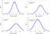 |
Fig. 6. Temperature function of the clusters from the mg − t analysis in four redshift bins. Lines and conventions are as in Fig. 5. |
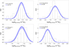 |
Fig. 7. Gas mass function of the clusters from the l − mg analysis in four redshift bins. Lines and conventions are as in Fig. 5. |
As long as the tails of the covariate distributions are accounted for, conditional scatter and parameters of the scaling relations are well recovered (Kelly 2007; Sereno 2016). A simple normal distribution provides reliable results since it can simultaneously account for the selection effects that penalise low-signal clusters and for the rarity of high-mass clusters (Lima & Hu 2005; Sereno & Ettori 2015a). A covariate distribution following the halo mass function would fail to reproduce the suppression at the low-mass end.
7. Previous results
Intrinsic scatter and correlation can be mass and time-dependent (Truong et al. 2018), and results from different samples should be compared cautiously. We also have to consider differences in measurements and definitions, mostly when comparing relations for either core-excised or core-included quantities. Furthermore, our sample extends to small groups, whereas most of the previous analyses considered more massive clusters. Finally, the present level of statistical uncertainties is too large to make firm conclusions on apparent disagreements. However, the positive correlation found with the analysis of XXL-100-GC is consistent with previous results. Maughan (2014) applied the PICACS model to two X-ray samples of clusters with T ≳ 2 keV with measured core-excised temperatures, gas masses, and either hydrostatic masses or luminosities. Quantities were measured within r500. The analysis suggested a positive correlation between the intrinsic scatter of T and Mg (ρmgt|m = 0.31 ± 0.30), and between T and the core excluded bolometric luminosity (ρtlce|m = 0.37 ± 0.30). A strong and significant correlation between the scatter in Mg and LX was found (ρlcemg|m = 0.85 ± 0.14).
Mantz et al. (2015) constrained the cosmological parameters through the analysis of the mass function of a sample of X-ray selected massive clusters (T ≳ 4 keV) detected in the ROSAT All-Sky Survey. They used follow-up measurements of soft band X-ray luminosity, temperature, and gas mass within r500 and weak gravitational lensing measurements of a sub-sample of massive clusters. In the process, they assumed the gas mass scatter as being uncorrelated, i.e. they fixed the off-diagonal covariance terms involving mg to zero, and measured the correlation ρtl|m = 0.11 ± 0.19. However, just using a larger amount of follow-up measurements and an updated calibration for X-ray observations, Mantz et al. (2016b) found a positive strong correlation in the intrinsic scatter of luminosity and temperature at fixed mass (ρtl|m = 0.53 ± 0.10).
Mantz et al. (2016a) studied the thermodynamic quantities of 40 massive clusters with T ≳ 5 keV identified as being dynamically relaxed and hot. Because the clusters were relaxed, they identified the hydrostatic mass with the true mass and measured the off-diagonal terms of the scatter covariance matrix. They considered gas mass, core-excised temperature, and core-excised or core-included soft-band [0.1–2.4] keV luminosity within r500. They found ρtl|m = −0.06 ± 0.24 and ρtmg|m = −0.18 ± 0.28, consistent with zero, and positive correlation between the core-included luminosity and the gas mass, ρlmg|m = 0.43 ± 0.22. The correlation is even stronger considering core-excised luminosity, ρlcemg|m = 0.88 ± 0.06.
Based on the analysis of 12 Local Cluster Substructure Survey (LoCuSS) massive clusters with T ≳ 5 keV, Okabe et al. (2010) derived a 68.3% confidence lower limit of ρtmg|m = 0.185, suggesting positive correlation between temperature and gas mass.
We caution that there are two main reasons why the slope and normalisation of the scaling relations studied here cannot be straightforwardly compared to most literature results. First, we consider quantities within fixed physical radii rather than within r500. Second, we are interested in model variables and we consider scatter in both the X and the Y variables. The luminosity-temperature relation determined in XXL Paper III, for example, is the relation between the intrinsic luminosity and temperature and the related scatter measures the dispersions of the luminosities at a given temperature. The l − t studied here is the hypothetical relation we would measure if temperature and luminosity were unscattered. This is the relation to study if we want to find the less scattered proxy since scatter values are measured with respect to a basic third property. Similar considerations apply to the gas mass-temperature relation and XXL Paper XIII.
Notwithstanding the previous caveats, our results compare well with other recent studies. The l − t and the mg − t relations for the XXL-100-GC sample were analysed by XXL Paper III and XXL Paper XIII, which we refer to for detailed analysis and review of literature results. Taking into account selection effects, XXL Paper III found a bolometric luminosity-temperature relation steeper than the self-similar expectation. XXL Paper XIII found a gas mass-temperature relation steeper than the self-similar expectation, with a slope in agreement with Arnaud et al. (2007), who analysed ten nearby relaxed clusters. Lovisari et al. (2015) analysed XMM-Newton observations for a complete sample of local (z < 0.034), flux-limited galaxy groups selected from the ROSAT All-Sky. They found a steeper than self-similar luminosity-temperature relation and a luminosity-gas mass relation compatible with expectations. Kettula et al. (2015) investigated groups from the XMM-CFHTLS survey together with high-mass systems from the Canadian Cluster Comparison Project and low-mass systems from the Cosmic Evolution Survey to find a steep luminosity-temperature relation.
8. Conclusions
Advancements in statistical methods applied to cluster physics have made possible the detailed study of scaling relations. The CoMaLit approach exploited in the present paper shares important features with other Bayesian methods (e.g. Kelly 2007; Okabe et al. 2010; Rozo et al. 2010; Evrard et al. 2014; Andreon & Congdon 2014; Maughan 2014; Mantz et al. 2015). The common theory behind these approaches includes the distinction of measured values, intrinsic scattered values, and model values; the modelling of the scaling relations as conditional probabilities; and the modelling of the completeness function of the sample in terms of the intrinsic distributions of the underlying quantities. Some important differences can arise from the treatment of the time evolution of scaling and scatter; the treatment of uncertainties, scatter, and covariances; the modelling of the distribution of the covariate variable; the treatment of selection biases; and the adopted priors.
Our analysis did not require knowledge of the mass, the assumption of hydrostatic equilibrium, or spherical symmetry. We only assumed that the matter halos that host clusters of galaxies have X-ray observable properties that are log-normally distributed around power-law scaling relations in halo mass.
We may think of the basic cluster property Z as a “mass substitute”, i.e. the best statistical quantity to use when we have no access to total mass. It should be the quantity with the strongest correlation to the studied properties. In principle, this ideal quantity may be fictitious. Only direct measurements of the cluster masses can eliminate any ambiguity or doubt. However, theoretical considerations based on the self-similar model, numerical simulations, and analyses of cluster samples with measured mass support the simplest hypothesis that Z is the mass.
We studied the scaling relations between X-ray properties of the XXL-100-GC sample and the intrinsic conditional scatter without any external mass calibration. In particular, we considered the spectroscopic temperature, the soft-band luminosity, and the gas mass within fixed physical radii. The sample spans one order of magnitude in temperature from small groups at T ∼ 0.6 keV to more massive clusters at T ∼ 7 keV. This probes the lower end of the halo mass function at the group scale, whereas most of previous analyses focused on more massive clusters (T ≳ 4 keV). The gas mass can be confirmed as an excellent proxy. Even when measured within a fixed physical length, cluster properties can be recovered from gas masses with ∼8%.
It should be noted that the gas mass is an equal or even better proxy than the weak lensing mass, which has an intrinsic scatter of σWL ∼ 15% (CoMaLit-I; Mantz et al. 2015) and a better proxy than the hydrostatic mass, σHE ∼ 25% CoMaLit-I.
We considered only a subsample of X-ray properties. Other proposals for mass proxies can be appealing too. The integrated SZ Compton parameter YSZ is expected to be tightly correlated to the energy content and the total mass of the clusters (Sereno & Ettori 2015a), but its measurements can be elusive for small systems. The product of the temperature and Mgas, 500, YX, is viewed as a robust mass indicator with low scatter (Kravtsov et al. 2006). However, this proxy performs best if the temperature is core-excised, which is not practical in small groups. Furthermore, any positive correlation between intrinsic scatter of temperature and gas mass, as found in this paper, can worsen its performance.
Multi-probe analyses can open new windows on the evolution and formations of structures (Sereno et al. 2018). Halo properties can be better understood in terms of multi-dimensional plans than basic one-to-one relations (Fujita et al. 2018). Generalised scaling laws suitably weighting X-ray observables have to be considered to calibrate the proxy with the minimum scatter (Ettori 2013).
We retrieved positive correlation between measured gas mass, temperature, and luminosity. The study of covariance between intrinsic scatter values is important as it impacts the propagation of selection biases based on one observable to biases on other observable quantities (Maughan 2014). For example, without taking the covariance between luminosity and gas mass or temperature into account, cluster masses estimated from Mg or T in an X-ray flux-limited sample would be biased high, with implications for cosmological studies (Maughan 2014).
The simple assumption of underlying power-law relations is enough to estimate the intrinsic scatter of the observed properties and rank them. However, the loop cannot be closed without the mass information. This is needed to calibrate the scaling relation and confirm that the optimal cluster proxy is indeed the optimal mass proxy.
The package LInear Regression in Astronomy (LIRA) is publicly available from Comprehensive R Archive Network (CRAN) at https://cran.r-project.org/web/packages/lira/index.html
Just Another Gibbs Sampler (JAGS) is a program for Bayesian data analysis publicly available at http://mcmc-jags.sourceforge.net/
Acknowledgments
XXL is an international project based around an XMM Very Large Programme surveying two 25 deg2 extragalactic fields at a depth of ∼5 × 10⁻¹⁵ erg cm−2 s−1 in the [0.5–2] keV band for point-like sources. The XXL website is http://irfu.cea.fr/xxl/. Multi-band information and spectroscopic follow-up of the X-ray sources are obtained through a number of survey programmes, summarised at http://xxlmultiwave.pbworks.com/. MS and SE acknowledge the financial contribution from the contract ASI-INAF n.2017-14-H.0. The Saclay group acknowledges long-term support from the Centre National d’Etudes Spatiales (CNES). This research has made use of NASA’s Astrophysics Data System (ADS) and of the NASA/IPAC Extragalactic Database (NED), which is operated by the Jet Propulsion Laboratory, California Institute of Technology, under contract with the National Aeronautics and Space Administration.
References
- Adami, C., Giles, P., Koulouridis, E., et al. 2018, A&A, 620, A5 (XXL Survey, XX) [NASA ADS] [CrossRef] [EDP Sciences] [Google Scholar]
- Andreon, S. 2012, A&A, 546, A6 [NASA ADS] [CrossRef] [EDP Sciences] [Google Scholar]
- Andreon, S., & Congdon, P. 2014, A&A, 568, A23 [NASA ADS] [CrossRef] [EDP Sciences] [Google Scholar]
- Angulo, R. E., Springel, V., White, S. D. M., et al. 2012, MNRAS, 426, 2046 [CrossRef] [Google Scholar]
- Arnaud, M., Pointecouteau, E., & Pratt, G. W. 2007, A&A, 474, L37 [NASA ADS] [CrossRef] [EDP Sciences] [Google Scholar]
- Arnaud, M., Pratt, G. W., Piffaretti, R., et al. 2010, A&A, 517, A92 [NASA ADS] [CrossRef] [EDP Sciences] [Google Scholar]
- Battaglia, N., Bond, J. R., Pfrommer, C., & Sievers, J. L. 2012, ApJ, 758, 74 [NASA ADS] [CrossRef] [Google Scholar]
- Bleem, L. E., Stalder, B., de Haan, T., et al. 2015, ApJS, 216, 27 [NASA ADS] [CrossRef] [Google Scholar]
- Eckert, D., Ettori, S., Coupon, J., et al. 2016, A&A, 592, A12 (XXL Survey, XIII) [NASA ADS] [CrossRef] [EDP Sciences] [Google Scholar]
- Ettori, S. 2013, MNRAS, 435, 1265 [NASA ADS] [CrossRef] [Google Scholar]
- Ettori, S. 2015, MNRAS, 446, 2629 [NASA ADS] [CrossRef] [Google Scholar]
- Ettori, S., Morandi, A., Tozzi, P., et al. 2009, A&A, 501, 61 [NASA ADS] [CrossRef] [EDP Sciences] [Google Scholar]
- Evrard, A. E., Arnault, P., Huterer, D., & Farahi, A. 2014, MNRAS, 441, 3562 [NASA ADS] [CrossRef] [Google Scholar]
- Fabjan, D., Borgani, S., Rasia, E., et al. 2011, MNRAS, 416, 801 [NASA ADS] [CrossRef] [Google Scholar]
- Feigelson, E. D., & Babu, G. J. 2012, Modern Statistical Methods for Astronomy (Cambridge: Cambridge Univ. Press) [Google Scholar]
- Fujita, Y., Umetsu, K., Ettori, S., et al. 2018, ApJ, 863, 37 [NASA ADS] [CrossRef] [Google Scholar]
- Gavazzi, R. 2005, A&A, 443, 793 [NASA ADS] [CrossRef] [EDP Sciences] [Google Scholar]
- Giles, P. A., Maughan, B. J., Pacaud, F., et al. 2016, A&A, 592, A3 (XXL Survey, III) [NASA ADS] [CrossRef] [EDP Sciences] [Google Scholar]
- Giodini, S., Lovisari, L., Pointecouteau, E., et al. 2013, Space Sci. Rev., 177, 247 [NASA ADS] [CrossRef] [Google Scholar]
- Hartley, W. G., Gazzola, L., Pearce, F. R., Kay, S. T., & Thomas, P. A. 2008, MNRAS, 386, 2015 [NASA ADS] [CrossRef] [Google Scholar]
- Hinshaw, G., Larson, D., Komatsu, E., et al. 2013, ApJS, 208, 19 [NASA ADS] [CrossRef] [Google Scholar]
- Kaiser, N. 1986, MNRAS, 222, 323 [NASA ADS] [CrossRef] [Google Scholar]
- Kelly, B. C. 2007, ApJ, 665, 1489 [NASA ADS] [CrossRef] [Google Scholar]
- Kettula, K., Giodini, S., van Uitert, E., et al. 2015, MNRAS, 451, 1460 [NASA ADS] [CrossRef] [Google Scholar]
- Kravtsov, A. V., Vikhlinin, A., & Nagai, D. 2006, ApJ, 650, 128 [NASA ADS] [CrossRef] [Google Scholar]
- Laureijs, R., Amiaux, J., Arduini, S., et al. 2011, ArXiv e-prints [arXiv:1110.3193] [Google Scholar]
- Lieu, M., Smith, G. P., Giles, P. A., et al. 2016, A&A, 592, A4 (XXL Survey, IV) [NASA ADS] [CrossRef] [EDP Sciences] [Google Scholar]
- Lima, M., & Hu, W. 2005, Phys. Rev. D, 72, 043006 [NASA ADS] [CrossRef] [Google Scholar]
- Limousin, M., Morandi, A., Sereno, M., et al. 2013, Space Sci. Rev., 177, 155 [NASA ADS] [CrossRef] [Google Scholar]
- Lovisari, L., Reiprich, T. H., & Schellenberger, G. 2015, A&A, 573, A118 [NASA ADS] [CrossRef] [EDP Sciences] [Google Scholar]
- Mantz, A. B. 2016, MNRAS, 457, 1279 [NASA ADS] [CrossRef] [Google Scholar]
- Mantz, A., Allen, S. W., Rapetti, D., & Ebeling, H. 2010, MNRAS, 406, 1759 [NASA ADS] [Google Scholar]
- Mantz, A. B., von der Linden, A., Allen, S. W., et al. 2015, MNRAS, 446, 2205 [NASA ADS] [CrossRef] [Google Scholar]
- Mantz, A. B., Allen, S. W., Morris, R. G., & Schmidt, R. W. 2016a, MNRAS, 456, 4020 [NASA ADS] [CrossRef] [Google Scholar]
- Mantz, A. B., Allen, S. W., Morris, R. G., et al. 2016b, MNRAS, 463, 3582 [NASA ADS] [CrossRef] [Google Scholar]
- Marulli, F., Veropalumbo, A., Sereno, M., et al. 2018, A&A, 620, A1 (XXL Survey, XVI) [NASA ADS] [CrossRef] [EDP Sciences] [Google Scholar]
- Maturi, M., Bellagamba, F., Radovich, M., et al. 2019, MNRAS, 485, 498 [NASA ADS] [CrossRef] [Google Scholar]
- Maughan, B. J. 2007, ApJ, 668, 772 [NASA ADS] [CrossRef] [Google Scholar]
- Maughan, B. J. 2014, MNRAS, 437, 1171 [NASA ADS] [CrossRef] [Google Scholar]
- Maughan, B. J., Giles, P. A., Randall, S. W., Jones, C., & Forman, W. R. 2012, MNRAS, 421, 1583 [NASA ADS] [CrossRef] [Google Scholar]
- Melchior, P., Gruen, D., McClintock, T., et al. 2017, MNRAS, 469, 4899 [NASA ADS] [CrossRef] [Google Scholar]
- Mohr, J. J., Mathiesen, B., & Evrard, A. E. 1999, ApJ, 517, 627 [NASA ADS] [CrossRef] [Google Scholar]
- Oguri, M., Takada, M., Umetsu, K., & Broadhurst, T. 2005, ApJ, 632, 841 [NASA ADS] [CrossRef] [Google Scholar]
- Okabe, N., Zhang, Y.-Y., Finoguenov, A., et al. 2010, ApJ, 721, 875 [NASA ADS] [CrossRef] [Google Scholar]
- Pacaud, F., Clerc, N., Giles, P. A., et al. 2016, A&A, 592, A2 (XXL Survey, II) [NASA ADS] [CrossRef] [EDP Sciences] [Google Scholar]
- Pacaud, F., Pierre, M., Melin, J.-B., et al. 2018, A&A, 620, A10 (XXL Survey, XXV) [NASA ADS] [CrossRef] [EDP Sciences] [Google Scholar]
- Pierre, M., Pacaud, F., Adami, C., et al. 2016, A&A, 592, A1 (XXL Survey, I) [NASA ADS] [CrossRef] [EDP Sciences] [Google Scholar]
- Planck Collaboration XX. 2014, A&A, 571, A20 [NASA ADS] [CrossRef] [EDP Sciences] [Google Scholar]
- Planck Collaboration XXIX. 2014, A&A, 571, A29 [NASA ADS] [CrossRef] [EDP Sciences] [Google Scholar]
- Pratt, G. W., Croston, J. H., Arnaud, M., & Böhringer, H. 2009, A&A, 498, 361 [NASA ADS] [CrossRef] [EDP Sciences] [Google Scholar]
- Rasia, E., Meneghetti, M., Martino, R., et al. 2012, New J. Phys., 14, 055018 [NASA ADS] [CrossRef] [Google Scholar]
- Rowley, D. R., Thomas, P. A., & Kay, S. T. 2004, MNRAS, 352, 508 [NASA ADS] [CrossRef] [Google Scholar]
- Rozo, E., Wechsler, R. H., Rykoff, E. S., et al. 2010, ApJ, 708, 645 [NASA ADS] [CrossRef] [Google Scholar]
- Rozo, E., Bartlett, J. G., Evrard, A. E., & Rykoff, E. S. 2014, MNRAS, 438, 78 [NASA ADS] [CrossRef] [Google Scholar]
- Saro, A., Mohr, J. J., Bazin, G., & Dolag, K. 2013, ApJ, 772, 47 [CrossRef] [Google Scholar]
- Sereno, M. 2007, MNRAS, 380, 1207 [NASA ADS] [CrossRef] [Google Scholar]
- Sereno, M. 2016, MNRAS, 455, 2149 [NASA ADS] [CrossRef] [Google Scholar]
- Sereno, M., & Ettori, S. 2015a, MNRAS, 450, 3675 [NASA ADS] [CrossRef] [Google Scholar]
- Sereno, M., & Ettori, S. 2015b, MNRAS, 450, 3633 [NASA ADS] [CrossRef] [Google Scholar]
- Sereno, M., & Ettori, S. 2017, MNRAS, 468, 3322 [NASA ADS] [CrossRef] [Google Scholar]
- Sereno, M., & Umetsu, K. 2011, MNRAS, 416, 3187 [NASA ADS] [CrossRef] [Google Scholar]
- Sereno, M., Ettori, S., Umetsu, K., & Baldi, A. 2013, MNRAS, 428, 2241 [NASA ADS] [CrossRef] [Google Scholar]
- Sereno, M., Ettori, S., & Moscardini, L. 2015, MNRAS, 450, 3649 [NASA ADS] [CrossRef] [Google Scholar]
- Sereno, M., Umetsu, K., Ettori, S., et al. 2018, ApJ, 860, L4 [NASA ADS] [CrossRef] [Google Scholar]
- Stanek, R., Rasia, E., Evrard, A. E., Pearce, F., & Gazzola, L. 2010, ApJ, 715, 1508 [NASA ADS] [CrossRef] [Google Scholar]
- Torri, E., Meneghetti, M., Bartelmann, M., et al. 2004, MNRAS, 349, 476 [NASA ADS] [CrossRef] [Google Scholar]
- Truong, N., Rasia, E., Mazzotta, P., et al. 2018, MNRAS, 474, 4089 [NASA ADS] [CrossRef] [Google Scholar]
- Vikhlinin, A., Burenin, R. A., Ebeling, H., et al. 2009a, ApJ, 692, 1033 [NASA ADS] [CrossRef] [Google Scholar]
- Vikhlinin, A., Kravtsov, A. V., Burenin, R. A., et al. 2009b, ApJ, 692, 1060 [NASA ADS] [CrossRef] [Google Scholar]
Appendix A: Asymmetric errors
The likelihood function of the measured spectroscopic temperature is approximately Gaussian in log space (XXL Paper III). We use the method of Andreon (2012) to convert the asymmetric errors on T computed by XSPEC to symmetric errors on log T. If the probability distribution p(T) is approximately log-normal, the standard deviation of the distribution p(log T) is given by
 (A.1)
(A.1)
where Tmode is the mode and the uncertainties δ+ and δ− are the points where the likelihood is lower than its maximum by a factor exp(−1/2).
Under the same assumption, we extend the prescription of Andreon (2012) and we also compute the mean as
 (A.2)
(A.2)
Appendix B: 2D posteriors
The marginalised 2D posterior probabilities for the luminosity-temperature, gas mass-temperature, and luminosity-gas mass relations are plotted in Figs. B.1–B.3. The results for the multi-response regression are shown in Fig. B.4.
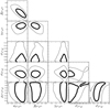 |
Fig. B.1. Probability distributions of the parameters of the scaling relation between luminosity and temperature: l − t. The thick (thin) lines include the 1σ(2σ) confidence region in two dimensions, here defined as the region within which the probability is higher than exp[−2.3/2] (exp[−6.17/2]) of the maximum. |
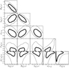 |
Fig. B.2. Probability distributions of the parameters of the scaling relation between gas mass and temperature: mg − t. The thick (thin) contours include the 1σ(2σ) confidence region in two dimensions, here defined as the region within which the probability is higher than exp[−2.3/2] (exp[−6.17/2]) of the maximum. |
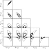 |
Fig. B.3. Probability distributions of the parameters of the scaling relation between luminosity and gas mass: l − mg. The thick (thin) contours include the 1σ(2σ) confidence region in two dimensions, here defined as the region within which the probability is higher than exp[−2.3/2] (exp[−6.17/2]) of the maximum. |
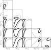 |
Fig. B.4. Probability distributions of the scatter parameters from the multi-response regression. The thick (thin) contours include the 1σ(2σ) confidence region in two dimensions, here defined as the region within which the probability is higher than exp[−2.3/2] (exp[−6.17/2]) of the maximum. |
All Tables
All Figures
|
Fig. 1. Graphic view of some quantities playing in the Bayesian regression scheme, see Sect. 2: the measurement results (blue); the true property values (red); the rescaled values of a basic feature (black). |
| In the text | |
|
Fig. 2. Scaling relations. The black points indicate the data, the blue lines represent the fitted scaling relation at the median redshift. The dashed blue lines show the median scaling relation (solid blue line) plus or minus the intrinsic scatter σY|Z. The shaded blue region encloses the 68.3% confidence region around the median due to uncertainties on the scaling parameters. The red line shows the self-similar prediction. Top panel: scaling between luminosity and temperature: l − t. Middle panel: scaling between gas mass and temperature: mg − t. Bottom panel: scaling between luminosity and gas mass: l − mg. |
| In the text | |
|
Fig. 3. Inferred probability density functions of the conditional intrinsic scatter with respect to the mass substitute. The blue and the green lines show the results based on the fits of pairs; the orange and the red lines show the densities obtained with the joint analysis of pair fits and with the multi-response regression, respectively. Top panel: gas mass intrinsic scatter. Middle panel: temperature intrinsic scatter. Bottom panel: luminosity intrinsic scatter. |
| In the text | |
|
Fig. 4. Time dependence of the X-ray observables of the selected clusters. Measured values are shown as a function of redshift (black points). The full lines plot the value of the unscattered observable below which a given fraction of the selected sample is contained. From top to bottom, the red, green, and blue lines show the 85%, 50%, and 15% levels (μZ), respectively. The shaded green region encloses the 68.3% confidence region around μZ(z) due to uncertainties on the parameters. Top panel: time dependence of the temperatures as inferred from the l − t relation. Temperatures are in units of keV. Middle panel: time dependence of the distribution of temperatures of the selected clusters as inferred from the mg − t relation. Bottom panel: time dependence of the distribution of gas masses of the selected clusters as inferred from the l − mg relation. Masses are in units of 1014 M⊙. |
| In the text | |
|
Fig. 5. Temperature function of the clusters from the l − t analysis in four redshift bins. The black histogram groups the observed temperatures. The blue line is the normal approximation estimated from the regression at the median redshift in the bin. The shaded blue region encloses the 68.3% probability region around the median relation due to uncertainties on the parameters. The function for the observed temperatures is estimated from the regression output, i.e. the function of the unscattered temperatures, by smoothing the prediction with a Gaussian whose variance is given by the quadratic sum of the intrinsic scatter of the (logarithmic) temperature with respect to the unscattered temperature and the median observational uncertainty. Redshift increases clockwise from the top left to the bottom left panel. The median and the boundaries of the redshift bins are indicated in the legends of the respective panels. |
| In the text | |
|
Fig. 6. Temperature function of the clusters from the mg − t analysis in four redshift bins. Lines and conventions are as in Fig. 5. |
| In the text | |
|
Fig. 7. Gas mass function of the clusters from the l − mg analysis in four redshift bins. Lines and conventions are as in Fig. 5. |
| In the text | |
|
Fig. B.1. Probability distributions of the parameters of the scaling relation between luminosity and temperature: l − t. The thick (thin) lines include the 1σ(2σ) confidence region in two dimensions, here defined as the region within which the probability is higher than exp[−2.3/2] (exp[−6.17/2]) of the maximum. |
| In the text | |
|
Fig. B.2. Probability distributions of the parameters of the scaling relation between gas mass and temperature: mg − t. The thick (thin) contours include the 1σ(2σ) confidence region in two dimensions, here defined as the region within which the probability is higher than exp[−2.3/2] (exp[−6.17/2]) of the maximum. |
| In the text | |
|
Fig. B.3. Probability distributions of the parameters of the scaling relation between luminosity and gas mass: l − mg. The thick (thin) contours include the 1σ(2σ) confidence region in two dimensions, here defined as the region within which the probability is higher than exp[−2.3/2] (exp[−6.17/2]) of the maximum. |
| In the text | |
|
Fig. B.4. Probability distributions of the scatter parameters from the multi-response regression. The thick (thin) contours include the 1σ(2σ) confidence region in two dimensions, here defined as the region within which the probability is higher than exp[−2.3/2] (exp[−6.17/2]) of the maximum. |
| In the text | |
Current usage metrics show cumulative count of Article Views (full-text article views including HTML views, PDF and ePub downloads, according to the available data) and Abstracts Views on Vision4Press platform.
Data correspond to usage on the plateform after 2015. The current usage metrics is available 48-96 hours after online publication and is updated daily on week days.
Initial download of the metrics may take a while.