| Issue |
A&A
Volume 631, November 2019
|
|
|---|---|---|
| Article Number | A77 | |
| Number of page(s) | 21 | |
| Section | Stellar structure and evolution | |
| DOI | https://doi.org/10.1051/0004-6361/201935160 | |
| Published online | 22 October 2019 | |
First grids of low-mass stellar models and isochrones with self-consistent treatment of rotation
From 0.2 to 1.5 M⊙ at seven metallicities from PMS to TAMS⋆
1
Department of Astronomy – University of Geneva, Chemin des Maillettes 51, 1290 Versoix, Switzerland
2
LUPM UMR 5299 CNRS/UM, Université de Montpellier, CC 72, 34095 Montpellier Cedex 05, France
3
University of Exeter, Department of Physics & Astronomy, Stoker Road, Devon, Exeter EX4 4QL, UK
e-mail: This email address is being protected from spambots. You need JavaScript enabled to view it.
4
IRAP, UMR 5277 CNRS and Université de Toulouse, 14 Av. E. Belin, 31400 Toulouse, France
5
Univ. Grenoble Alpes, CNRS, IPAG, 38000 Grenoble, France
6
Institut UTINAM, CNRS UMR 6213, Univ. Bourgogne Franche-Comté, OSU THETA Franche-Comté-Bourgogne, Observatoire de Besançon, BP 1615, 25010 Besançon Cedex, France
7
Institut d’Astronomie et d’Astrophysique, Université Libre de Bruxelles (ULB), CP226, Boulevard du Triomphe, 1050 Brussels, Belgium
Received:
29
January
2019
Accepted:
20
May
2019
Abstract
Aims. We present an extended grid of state-of-the art stellar models for low-mass stars including updated physics (nuclear reaction rates, surface boundary condition, mass-loss rate, angular momentum transport, rotation-induced mixing, and torque prescriptions). We evaluate the impact of wind braking, realistic atmospheric treatment, rotation, and rotation-induced mixing on the structural and rotational evolution from the pre-main sequence (PMS) to the turn-off.
Methods. Using the STAREVOL code, we provide an updated PMS grid. We computed stellar models for seven different metallicities, from [Fe/H] = −1 dex to [Fe/H] = +0.3 dex with a solar composition corresponding to Z = 0.0134. The initial stellar mass ranges from 0.2 to 1.5 M⊙ with extra grid refinement around one solar mass. We also provide rotating models for three different initial rotation rates (slow, median, and fast) with prescriptions for the wind braking and disc-coupling timescale calibrated on observed properties of young open clusters. The rotational mixing includes the most recent description of the turbulence anisotropy in stably stratified regions.
Results. The overall behaviour of our models at solar metallicity, and their constitutive physics, are validated through a detailed comparison with a variety of distributed evolutionary tracks. The main differences arise from the choice of surface boundary conditions and initial solar composition. The models including rotation with our prescription for angular momentum extraction and self-consistent formalism for angular momentum transport are able to reproduce the rotation period distribution observed in young open clusters over a wide range of mass values. These models are publicly available and can be used to analyse data coming from present and forthcoming asteroseismic and spectroscopic surveys such as Gaia, TESS, and PLATO.
Key words: stars: evolution / stars: rotation / stars: low-mass / stars: pre-main sequence
The model grid is only available at the CDS via anonymous ftp to cdsarc.u-strasbg.fr (130.79.128.5) or via http://cdsarc.u-strasbg.fr/viz-bin/cat/J/A+A/631/A77
© ESO 2019
1. Introduction
Along with mass and chemical composition, the angular momentum (AM) content is one of the fundamental characteristics of single stars (see the review by Maeder 2009). Rotation affects the whole stellar evolution from birth to death, with direct effects on the structure (e.g. Endal & Sofia 1976; Maeder & Meynet 2001; Roxburgh 2004; Rieutord 2006), mass-loss rate (e.g. Owocki & Gayley 1997; Langer 1998; Maeder & Meynet 2000; Georgy et al. 2011), evolutionary path in the Hertzsprung–Russell diagram, asteroseismic properties (e.g. Ballot et al. 2006; Eggenberger et al. 2010; Lagarde et al. 2012; Reese et al. 2013; Bouabid et al. 2013; Prat et al. 2017), lifetime, and internal and surface chemical composition of stars. It is also of crucial importance for potential life-hosting stellar systems because of the role played by rotation in generating magnetic fields by dynamo action (e.g. Noyes et al. 1984; Wright et al. 2011; Vidotto et al. 2014a; Johnstone et al. 2015a; Gallet et al. 2017; Brun & Browning 2017).
The case of low-mass stars is particularly interesting because their AM evolution involves various processes at different stages of their life. It starts with the collapse of the initial protostellar cloud in which jets and outflows remove of the order of 99% of the AM content on a dynamical timescale (see e.g. Mathieu 2004). Then magnetic interactions between the star and its surrounding disc, and later between the stellar wind and the star’s magnetic field, determine the star’s rotation velocity on the main sequence.
During the last decade, stellar evolution models have strongly benefited from high-quality photometry data from space missions, such as Kepler (see e.g. Borucki et al. 2010; Gilliland et al. 2010), and ground-based long-term monitoring surveys (see e.g. Bouvier et al. 2014, for a fairly complete overview). By providing accurate surface rotation periods for large samples of low-mass stars, and internal rotation profiles at some specific evolution phases by seismic analysis, these complementary observations have improved our knowledge of the physical processes driving the rotational evolution of stars.
Over the same period, special care was brought to the development of new models for AM losses due to magnetised winds in low-mass (see e.g. Pinto et al. 2011; Reiners & Mohanty 2012; Matt et al. 2012, 2015; van Saders & Pinsonneault 2013; Johnstone et al. 2015b; Réville et al. 2016; Pantolmos & Matt 2017; Garraffo et al. 2018) and massive stars (see e.g. Ud-Doula et al. 2009; Lau et al. 2011). Most of these prescriptions have been tested through post-processing computations of AM evolution based on pre-computed standard evolutionary tracks (see e.g. Gallet & Bouvier 2013, 2015; Johnstone et al. 2015c; Sadeghi Ardestani et al. 2017), hence ignoring the effects of rotation on the structure and the evolution of the star. This approach provides information on the magnitude of the torque and the degree of core-envelope coupling or decoupling at the different phases of the evolution, and the results are compatible with the observed rotation period distribution of stars in clusters. However, it does not probe the actual physical processes that transport AM in the interior.
To reach a more consistent picture over a broader range of mass and chemical composition, we implemented these magnetic wind braking models directly into our stellar evolution code that can self-consistently treat rotation-induced transport processes (e.g. meridional circulation and turbulence). We first applied this approach to solar-type stars in Amard et al. (2016). In that study, we searched for the best combinations of prescriptions for internal transport of AM and surface braking by magnetised stellar winds to account for the observed rotational periods in open clusters of different ages. We showed that the rotation period distributions can be successfully reproduced by models maintaining a certain amount of internal differential rotation even at late ages. We also confirmed that evolutionary models that only include AM transport by meridional circulation and turbulence, do not properly account for the rotation profile inside the Sun (Turck-Chièze et al. 2010; Marques et al. 2013), and the core rotation rates in subgiant and red giant stars (Eggenberger et al. 2012; Ceillier et al. 2012). These models also failed to reproduce the surface lithium abundances of solar-mass stars in young clusters (e.g. Sestito & Randich 2005; Talon & Charbonnel 2010; Somers & Stassun 2017). Currently, the consensus is that additional processes like internal gravity waves or magnetic fields (Charbonnel & Talon 2005; Eggenberger et al. 2005; Talon & Charbonnel 2008; Charbonnel et al. 2013; Li et al. 2014; Cantiello et al. 2014; Fuller et al. 2014; Belkacem et al. 2015; Jouve et al. 2015; Pinçon et al. 2017) might play an important role.
However, we have not yet fully investigated the complexity of rotation-driven hydrodynamical instabilities (see e.g. Mathis et al. 2018; Jermyn et al. 2018). Recently, we proposed an updated description of anisotropic turbulence in stellar radiative regions (Mathis et al. 2018) that induces a more efficient transport of AM than previous prescriptions. This prescription cannot yet reproduce the solid-body rotation profile at the age of the Sun, but links for the first time the anisotropy of the turbulent transport in radiation zones to their stratification and rotation. This is a major improvement that deserves a deeper investigation over a broad range of stellar masses and metallicities.
In the present grid of stellar models, we take into account current prescriptions for AM extraction by magnetised winds and AM transport by anisotropic turbulence. Our computations also include state-of-the-art model atmospheres and updated nuclear reaction rates. They cover the evolution from the pre-main sequence (PMS) to the main-sequence turn-off for stars with masses between 0.2 and 1.5 M⊙ and seven metallicities ([Fe/H] between −1 dex and +0.3 dex). For each mass-metallicity combination, we compute one non-rotating model (the so-called standard model), and three rotating models with different initial rotation rates (slow, median, and fast) and disc lifetimes to cover the dispersion of rotation periods observed for stars of different masses and ages. These stellar tracks are made available to the community, and we also provide the corresponding isochrones.
There are other grids of rotating stellar models with various initial metallicities (e.g. Lagarde et al. 2012; Ekström et al. 2012; Yang et al. 2013; Georgy et al. 2013; Choi et al. 2016); this work presents for the first time a discussion of the effects of varying both the initial mass and metallicity on the transport of AM in low-mass stars undergoing magnetic braking.
The paper is structured as follows. In Sect. 2, we describe the updated version of the STAREVOL code and present the various prescriptions used for input physics and our initial conditions. In Sect. 3 we describe the content of the CDS material and in Sect. 4 we compare our standard Z⊙ tracks to other models computed with different codes. In Sect. 5 we discuss the evolution of AM, and compare the predictions of the solar metallicity grid to observed rotation period distributions in open clusters. Finally, we present our conclusions in Sect. 6.
2. Stellar evolution code: STAREVOL v3.40
The models presented here were computed with the stellar evolution code STAREVOL. The widely used PMS grid by Siess et al. (2000) was already computed with an early version of this code, as were grids of low- and intermediate-mass stars (Forestini & Charbonnel 1997; Siess et al. 2002; Lagarde et al. 2012; Chantereau et al. 2015) and of SAGB stars (Siess 2007, 2010). Here we use the latest version of the code (v3.40) jointly developed at Geneva and Montpellier Universities, which is an update of version v3.30 used in Amard et al. (2016). We describe below the input prescriptions for the micro- and macro-physics of STAREVOL v3.40; in some cases we comment on the differences with respect to other grids from the literature (see also Sect. 4).
2.1. Initial abundances and opacities
We adopt the heavy elements mixture of Asplund et al. (2009), giving a reference value of solar photospheric metallicity Z = 0.013446. A calibration of the solar model with the present input physics leads to an initial helium mass fraction Y = 0.2691. We use the corresponding constant slope ΔY/ΔZ = 1.60 (with the primordial abundance Y0 = 0.2463 based on WMAP-SBBN by Coc et al. 2004) to set the initial helium mass fraction at a given metallicity Z. We account for α-element enrichments below [Fe/H] ≤ –0.3 dex following the Galactic chemical evolution trends by e.g. Fuhrmann (2011). The values are shown in Table 1. Compared to the Grevesse & Noels (1993) solar mixture used in Siess et al. (2000), the solar abundances of almost all elements heavier than helium, and especially of carbon, nitrogen, and oxygen, are significantly lower. Our initial chemical composition is slightly different from that of Lagarde et al. (2012), who also used the Asplund et al. (2009) heavy element mixture, because our solar calibration with updated physics leads to a higher solar helium mass fraction (Y = 0.2691 instead of 0.266) and helium-to-metals slope (ΔY/ΔZ = 1.60 instead of 1.29).
Chemical abundances and metallicities scaled according to the solar chemical mixture by Asplund et al. (2009).
Below 8000 K we use the Ferguson et al. (2005) opacities and above this temperature, the OPAL tables Iglesias & Rogers (1996). We use the same equation of state as described in Siess et al. (2000).
2.2. Nuclear reaction rates and network
The nuclear energy production is computed with a reaction network including 185 nuclear reactions involving 54 stable and unstable species from 1H to 37Cl. We essentially use the same rates as in Lagarde et al. (2012) except for nuclei with mass number A < 16, for which we adopt the updated rates from the NACRE II compilation (Xu et al. 2013a). The numerical tables used in the code are generated using the NetGen web interface1 (Xu et al. 2013b). The screening factors are calculated with the formalism of Mitler (1977) for weak and intermediate screening conditions and of Graboske et al. (1973) for strong screening conditions.
2.3. Treatment of the atmosphere
Special attention was given to the treatment of the stellar atmosphere. In the STAREVOL code, the stellar structure equations are solved in one shot from the centre to the surface; there is no decoupling between the interior and the atmosphere, as is done in some stellar evolution codes. The surface boundary conditions are treated using the Hopf function, q(τ), which provides at a given optical depth τ a correction to the grey approximation (see Hopf 1930; Morel et al. 1994)
 (1)
(1)
where Teff is the temperature of the equivalent black body and T(τ) the temperature profile. In the previous PMS grid, Siess et al. (2000) used analytical q(τ) expressions derived from tailored Kurucz and MARCS model atmospheres.
In the present study, the functions q(τ) are calculated from the values of T(τ) and Teff given by the PHOENIX atmosphere models (Allard et al. 2012). We selected these models2 because of their wide coverage in 2600 K ≤ Teff ≤ 70 000 K, 0 ≤ logg(cm s−2) ≤ +5.0 and −4.0≤ [M/H] ≤ + 0.5) and also because they adopt the same solar mixture (Asplund et al. 2009) and a mixing-length parameter value αc = 2.0 very close to ours of 1.973. The connection between the atmosphere and the interior can be done at a specific temperature (e.g. Feiden & Chaboyer 2012), or at a given optical depth τph (e.g. Tognelli et al. 2011; Chen et al. 2014; Baraffe et al. 2015). As shown in Montalbán et al. (2004), the result of the calculations does not depend sensitively on the location of the matching point provided it remains in a region where 10 < τph < 100. However, in STAREVOL, we consider that each point between τ = 30 and τ = 100 is a matching point. So, given the metallicity and surface gravity of the model, we search for the model atmosphere effective temperature that gives the stellar structure temperature at the matching point’s optical depth. We then calculate an average effective temperature from the previously computed values of Teff. Finally, we interpolate in the grid of model atmosphere the new temperature profile corresponding to the mean ⟨Teff⟩ and use Eq. (1) to obtain the expression of q(τ). This model atmosphere, which is calculated at each iteration during the convergence process, also provides the outer boundary condition on the density. In our calculations, we set the numerical surface to be at an optical depth τ = 0.015.
The effect of changing the surface boundary condition is illustrated in Fig. 1. The 1.5 M⊙ model is almost unaffected by the use of a realistic atmosphere model, except on the Hayashi track, where the tracks are 100 K cooler than in calculations using a grey atmosphere boundary condition. This difference is also present on the 1.0 M⊙ Hayashi track and remains along the main sequence. As expected, the colder the surface and hence the lower the stellar mass, the stronger the impact of the atmosphere on the structure and hence on the location of the tracks in the HRD. For the 0.5 M⊙ case, the difference between a model using a grey atmosphere and one using a PHOENIX atmosphere can exceed 300 K during the PMS and 200 K on the MS. We note that the models using the Krishna Swamy (1966) prescription fit quite well the evolution with PHOENIX atmosphere models at solar metallicity even in the low-mass regime.
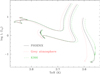 |
Fig. 1. Evolutionary tracks in the Hertzsprung–Russell diagram for standard models of 0.5, 1.0, and 1.5 M⊙ at Z⊙ from bottom to top using the three different boundary conditions indicated on the plot. KS66 refers to the Krishna Swamy (1966) prescription. |
2.4. Mixing-length parameter for convection
The use of new boundary conditions and new input physics requires a new calibration of the mixing-length parameter (and initial helium content, see Sect. 2.1) to reproduce the solar radius and luminosity at the current age of the Sun. We calibrated the luminosity and radius of a non-rotating 1.0 M⊙ model, neglecting mass loss, to a relative precision of 10−4. We obtain a mixing-length parameter value αc = 1.973 with a helium content Y = 0.269 for a metallicity Z = 0.0134 corresponding to the Asplund et al. (2009) mixture. We keep the same value of αc for all the models of the grid. In all our models, standard and rotating, overshooting is not considered.
2.5. Mass-loss prescriptions
We compute the mass-loss rate all along the evolution with two different prescriptions depending on whether it is a rotating model or not. In the non-rotating case, the mass-loss rate follows Reimers (1975) (with ηR = 0.5), while in the rotating case we use the mass-loss rate given by Cranmer & Saar (2011). The latter takes into account the effects of rotation on the stellar activity, and thus depends implicitly on the stellar spin. A metallicity scaling is applied to the mass-loss rate following Mokiem et al. (2007):
 (2)
(2)
2.6. Angular momentum evolution
2.6.1. Initial spin velocity
The initial models are build from polytropes and are all fully convective. We assume an initial solid-body rotation and consider three different initial rotation periods (Prot, init = 1.6, 4.5 and 9 days) for which we associate a disc-locking timescale. The values of τDC and Prot, init (see Table 3) are based on the study of Gallet & Bouvier (2015) and are chosen to reproduce the spread in rotation periods observed in young open clusters (see Gallet & Bouvier 2013, 2015; Amard et al. 2016; Sadeghi Ardestani et al. 2017). It should be noted that, in order to prevent the most massive stars (1.2–1.5 M⊙) from exceeding their critical velocity, we increased the initial rotation period from 1.6 to 2.3 days and the disc-coupling duration from 2.5 to 4 Myr for the fast-rotating models.
Our simplified treatment of disc coupling (τDC independent of mass and metallicity for a given Prot, init) implies that the rotation period remains constant during the first few million years of evolution. Our initial models can have very large radii, and for the initially fast rotators the spin acceleration following the star–disc unlocking may bring the star to break-up velocities. To avoid this non-physical situation, the models are evolved as non-rotating for the first five hundred thousand years (which sets the time zero of the evolution of our models) and only after this time is rotation taken into account. Such a precaution is not necessary for the median and slow rotators.
Finally, as in Amard et al. (2016), the effects of rotation on the structure are treated following the formalism of Endal & Sofia (1976).
2.6.2. Internal transport of angular momentum
We describe here the transport of AM in the stellar interior following the formalism of Zahn (1992) as updated by Maeder & Zahn (1998) and Mathis & Zahn (2004). The transport of AM happens on a secular timescale in the radiative regions of the star (see e.g. Decressin et al. 2009). As the star evolves, differential rotation develops in the radiative region that contributes to the transport of AM between the core and the envelope. We assume that the convective regions rotate as a solid body.
Based on the recent work on the anisotropy of turbulence in stellar radiative regions by Mathis et al. (2018), we modified the set of prescriptions for the turbulent diffusion coefficients compared to what was used in Amard et al. (2016). The horizontal turbulence (νh) is now the sum of two terms, one (νh, v) corresponding to the component created by the vertical shear, and one (νh, h) corresponding to the shear that develops along the isobar. The term νh, v is set to 0 when the vertical shear is not important enough to fulfil the Reynold’s criterion (i.e. νv ≥ νmRec, where Rec = 7; Prat, priv. comm.). For consistency with the expression of the horizontal turbulence, we use the Zahn (1992) prescription for the vertical shear-induced turbulence νv. These prescriptions do not require any parameter fine-tuning over the mass, rotation, and chemical composition ranges covered by our grid.
We recall the advection-diffusion equation for the transport of AM as given in Zahn (1992) and Mathis & Zahn (2004)
 (3)
(3)
where ρ, r, νv and Ur are the density, radius, vertical component of the turbulent viscosity, and the meridional circulation velocity on a given isobar, respectively. By integrating this equation at a given radius r we obtain a flux equation,
 (4)
(4)
with
 (5)
(5)
the flux carried by shear-induced turbulence from the radiative zone to the convective envelope (CE), and
 (6)
(6)
the flux carried by meridional circulation. A detailed derivation of the AM fluxes is given in Decressin et al. (2009) as part of a set of tools for assessing the relative importance of the processes involved in AM transport in stellar radiative interiors.
We would like to include a word of caution, however. The close-to-breakup stars and their internal transport are not expected to be rigorously modelled with our formalism because some assumptions are no longer fulfilled. More careful work would imply the use of two-dimensional simulations, which are not currently available for the considered evolutionary timescales (Espinosa Lara & Rieutord 2007; Hypolite et al. 2018).
2.6.3. Extraction of angular momentum
From the birthline to the terminal-age main sequence (TAMS), the AM content decreases by two orders of magnitude as the result of two main processes.
Disc coupling during early evolution. Young stars are spun up by contraction and accretion of AM through the circumstellar disc. They are also braked by the development of accretion-induced winds (Matt & Pudritz 2005, 2008; Zanni & Ferreira 2009), magnetospheric ejections (see e.g. Shu et al. 1994; Zanni & Ferreira 2013), or by the so-called disc-locking process (see e.g. Ghosh & Lamb 1979). Observations (Rebull et al. 2004; Gallet & Bouvier 2013) indicate that the interaction is very efficient and results in an almost constant stellar angular velocity during the disc lifetime. With this assumption of strong coupling, angular momentum evolution models (e.g. Bouvier et al. 2014) are able to reproduce the overall spread in surface velocities provided the disc lifetime is not unique.
As reported in several studies (Kennedy & Kenyon 2009; Williams & Cieza 2011; Vasconcelos & Bouvier 2017), the duration of the disc-locking phase is likely dependent on the stellar mass, initial rotation period (Gallet & Bouvier 2013), or stellar chemical composition (Ghezzi et al. 2018). In the absence of a clearer view, we use a unique disc-coupling timescale (τDC in Table 3) for all stars that depend only on the initial rotational period.
Additional AM loss due to magnetic wind braking is also considered throughout the evolution, as described in the following section.
Extraction of angular momentum by stellar winds. Low-mass stars with an external convective envelope sustain a dynamo-generated magnetic field, and thus undergo efficient magnetic braking during their evolution through their magnetised wind (e.g. Schatzman 1962). While the prescription by Kawaler (1988) has been extensively used to account for AM loss, recent theoretical studies (Reiners & Mohanty 2012; Matt et al. 2012, 2015; van Saders & Pinsonneault 2013; van Saders et al. 2016; Réville et al. 2015; Garraffo et al. 2018) provide a variety of “braking laws” that take into account various physical ingredients and are calibrated on different observational samples. In our models, the torque applied at the surface of the star is computed following Matt et al. (2015) formulation and writes
 (7)
(7)
 (8)
(8)
with
 (9)
(9)
where  comes from Eq. (8) of Matt et al. (2012), and u is the ratio of the surface velocity to the brake-up velocity. The calibration constant K is expected to be close to the solar wind torque derived from spin models (Finley et al. 2018), Ω⋆ is the surface angular velocity with J the stellar angular momentum; R⋆ and M⋆ denote the radius and stellar mass, and the symbol ⊙ indicates the solar value. This formalism depends on the Rossby number in the convective envelope (Nandy 2004; Jouve et al. 2010), defined as
 (10)
(10)
with τcz the turnover timescale estimated at 0.5 pressure scale height above the base of the convective envelope. In our model, the magnetic field saturates when Ro < Rosat and this saturation value is determined by imposing that our 1 M⊙ roughly reproduces the dispersion in rotation periods in the α-Per (≈ 85 Myr) and M 35 (≈150 Myr) open clusters. This requires  with Ro⊙ ∼ 2, and thus a saturation Rossby number Rosat = 0.14 very close to 0.13 ± 0.02 as observationally derived by Wright et al. (2011).
The question arises of whether it is realistic to derive convective velocities from a formalism as simple as the mixing-length theory. Multidimensional simulations of convection (Hanasoge et al. 2012; Viallet et al. 2013; Trampedach et al. 2014) have been showing that the mixing-length theory provides good estimates for convective velocities. This is particularly true close to the bottom of the convective envelope where we probe the convective turnover timescales, thus making our derived Rossby numbers more reliable.
In Amard et al. (2016), we used the parametric relation between Ro and the effective temperature, as suggested by Cranmer & Saar (2011). We refer the reader to Charbonnel et al. (2017) for a description of the variations of this quantity within the stellar convective envelope along the evolution and as a function of stellar mass and metallicity.
Torque calibration on observational constraints. With the updated physics, the constant K (Eq. (9)) had to be re-calibrated to reproduce the Sun’s rotation rate. We also calibrated by eye the value of p (Eqs. (7) and (8)) to match the observed velocity dispersion in the Pleiades and Praesepe clusters for the 1.0 M⊙ and 0.5 M⊙ models. The adopted values of the parameters K, p, m, and χ are given in Table 2 and are kept constant over the entire mass and metallicity range, independently of the initial rotational velocity.
Parameters used for Matt et al. (2015) prescription.
Grid parameters.
2.7. Transport of chemicals
In the rotating low-mass stars, rotation-induced mixing is expected to prevent the effect of atomic diffusion from becoming too large (see Deal et al. in prep.) because of the presence of a relatively thick surface convection zone. In these stars, the efficient braking of the surface by the magnetised stellar winds generates a strong shear below the convective envelope, responsible for an efficient mixing of the chemical species. For stars with a very shallow convective envelope, i.e. with a larger mass and/or lower metallicity, the differential rotation will be reduced and radiative levitation will become the main agent of chemical mixing (e.g. Richard et al. 2002). Since we do not account for gravitational settling or radiative levitation, the surface composition of our models with M > 0.8 M⊙ is not expected to be realistic (see Sect. 5.7). A full and consistent treatment of chemical transport including rotational induced mixing and atomic diffusion is one of our priorities for a forthcoming study.
The vertical transport of nuclides in the radiative regions results from the combined action of meridional circulation and turbulent shear whose formulation follows Chaboyer & Zahn (1992). For a chemical species i, the concentration ci obeys
 (11)
(11)
where Dtot = Deff + Dv is the total diffusion coefficient and Deff is given by
 (12)
(12)
where Dv and Dh is the vertical and horizontal turbulent diffusion coefficient, respectively. The term  accounts for the evolution of the concentration of chemical species i due to nuclear burning.
3. Description of the CDS tables
Our models have been integrated in the SYCLIST toolbox (Georgy et al. 2014). The published tables include 100 new points to describe the PMS evolution and adds two new key points to the list described in Ekström et al. (2012). The first defines the beginning of the pre-main-sequence phase (the point where the star is 105 yr old). The second indicates where the radiative core appears. We labelled them “0” and “0b”, so that point labelled “1”, defined as the zero age main sequence (ZAMS) where the star has burnt 0.003 hydrogen in mass fraction, is the same as in Ekström et al. (2012).
For each model, we selected a total of 290 points to allow a good description of the full tracks. We recall here the different evolutionary steps (see Fig. 2):
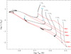 |
Fig. 2. Evolution track in the Hertzsprung–Russell diagram of six standard models of 0.2, 0.3, 0.5, 0.7, 1.0 and 1.5 M⊙ at solar metallicity. Isochrones corresponding to 1, 5, 10, 50 Myr and 1 Gyr are also represented in red. In blue are shown the evolutionary points described in the text. |
-
0
beginning of the pre-main sequence (1–20 pts);
-
0b
appearance of the radiative core if relevant (21–100 pts);
-
1
ZAMS (101–185 pts);
-
2
turning point with the lowest Teff on the main sequence (186–210 pts);
-
3
Main-sequence turn-off.
Point 0 exists for all models, as does point 1. Point 0b is not defined for very low-mass stars and in this case, we set it to same pre-main-sequence time fraction as in the lowest mass model (of the same metallicity and initial velocity) where it appears. There are 18 points between point 0 and point 0b, regularly spaced in terms of log(L), so that point 0b is the 20th point in the table. We then put 80 other points between point 0b and point 1, so that the ZAMS (which is the first point in the Ekström et al. 2012 tables) is now the 101st point in the table. The points between point 0b and point 1 are equally spaced in time. For stars that do not reach the turn-off by 15 Gyr, we set point 3 to the last computed point; point 2 is set as the last computed point for stars that do not reach the main sequence within 15 Gyr. For each model, the quantities given in Table A.1 can be retrieved from the Geneva webpage3. We also provide the conversion of each track into two photometric systems. The conversion in Gaia colours comes from Evans et al. (2018) and that in the Johnson-Cousin system follow Worthey & Lee (2011).
3.1. Asteroseismic quantities
All our stars have a convective envelope during the main sequence that is expected to generate solar-like oscillations. Following Lagarde et al. (2012), we provide different global asteroseismic parameters listed in Table A.1 that are computed from the structural properties of the models at each time step. They include a number of scaling relations: the large separation from scaling relation
 (13)
(13)
the frequency with the maximum amplitude
 (14)
(14)
and the maximum amplitude
 (15)
(15)
with Δν⊙ = 134.9 μHz, νmax, ⊙ = 3150 μHz, and Amax, ⊙ = 2.5 ppm the solar values.
Some asymptotic asteroseismic quantities are also provided: the asymptotic large separation
 (16)
(16)
with R the stellar radius and cs the sound speed; the total acoustic radius (T),
 (17)
(17)
the acoustic radii at the base of the CE (tBCE) and at the location of the helium second-ionisation region (tHe),
 (18)
(18)
with rBCE and rHe the stellar radius at the base of the CE and of the helium second-ionisation region, respectively. Finally, the asymptotic period spacing of g-mode defined as
 (19)
(19)
where r1 and r2 are the radii that define the cavity where the g-modes are trapped and N is the Brunt–Väisälä frequency. For more details, see the original article.
3.2. Isochrones
We also provide the possibility to compute isochrones in different spectral bands with different filters. These isochrones are computed using the SYCLIST tool and the reader is referred to Georgy et al. (2014) for corresponding details.
4. Comparison with other grids at solar metallicity
The important updates in the physics of the STAREVOL code since Siess et al. (2000) (see Lagarde et al. 2012 and Sect. 2) justifies the computation of a new set of grids. Moreover, over the past few years several research groups have published PMS evolutionary models. A comparison is therefore timely and will allows an assessment of the uncertainties in terms of HR diagram positions and ages associated with the use of different codes and input physics.
In Table 4 we compile the main physical assumptions used in the computation of publicly available stellar evolutionary tracks. These models are standard (i.e. non-rotating) and cover our grid mass range. In this table, the chemical mixture (Col. 2) refers to the adopted solar metallicity (Z). We also provide the initial helium mass fraction Y and the mixing-length parameter αMLT (Cols. 2 and 3, respectively). The solar symbol ⊙ in Col. 3 indicates the grids that use a calibration of their solar model (in terms of luminosity and radius at the age of the Sun) to determine Y and αMLT. In Col. 4 we indicate the set of model atmospheres used as external boundary condition and the optical depth where they are attached to the stellar interior. The adopted equation of state (EOS) is given in Col. 5; the importance of its accuracy for PMS stars has been largely discussed in the literature (e.g. Baraffe et al. 1998; Siess et al. 2000). In Col. 6 we recall the bibliographical sources for radiative opacities at high (first line) and low (second line) temperatures. Most of the current evolution codes use OPAL radiative opacities tables for the interior computation where T > 8000 K, but for T < 8000 K, two main opacity tables are considered: Alexander & Ferguson (1994) and Ferguson et al. (2005). Column 7 gives the source for the nuclear reaction rates while information about the use (or not) of core overshooting in the grid computation is given in Col. 8. The last two columns of the table give the age of the 1 M⊙, Z⊙ of each grid at the ZAMS and TAMS (see definition in the table notes) in Gyr, and the radius of this model at the ZAMS in units of R⊙.
ZAMS: Xc = 0.998Xc, i and TAMS: Xc < 0.002Xc, i.
Below we compare in more detail our grid of solar metallicity, standard, non-rotating models with the ones listed in Table 4. We find good agreement with most of them (especially FRANEC and MESA), as clearly visible from Fig. 3 where we plot selected evolution tracks in the Hertzsprung–Russell diagram. There is a systematic offset between our 0.2 M⊙ model and others that we think is due to the new treatment of the upper part of the atmosphere that we use.
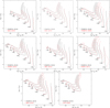 |
Fig. 3. Comparison of our standard solar metallicity models with other available grids as described in Table 4 and indicated in each panel. |
4.1. STAREVOL: Siess et al. (2000)
The Siess et al. (2000) grid has been extensively used for two decades. Due to the important improvements of the constitutive physics during that period of time, this oldest grid is also the one for which we find the largest discrepancies with our new models. This can be explained by the combined use of the Grevesse & Noels (1993) solar reference abundances, with an associated metallicity Z = 0.02 much higher than our adopted value of Z = 0.0134, a smaller MLT parameter α, and older atmosphere models used as boundary condition. For any given initial stellar mass, the Siess et al. (2000) models are cooler than ours and the Henyey tracks are always shorter. This behaviour has already been discussed in Montalbán et al. (2004), who conclude that it is essentially due to an interplay between the mixing-length parameter, the chemical composition, and the peculiar atmosphere models.
4.2. BHAC: Baraffe et al. (2015)
The models by Baraffe et al. (2015; hereafter BHAC) are an updated version of Baraffe et al. (1998) computed with an improved atmospheric treatment and the solar chemical mixture derived by Caffau et al. (2011). Baraffe et al. (1998) were the first group to publish models that self-consistently couple the stellar interiors and state-of-the-art atmosphere models, therefore becoming a reference for low-mass stellar evolution models. This approach has since been adopted by other groups, including ours. The BHAC grid ensures the consistency of the convection treatment between the interior and the atmosphere, with a calibrated mixing-length parameter. Figure 3 shows that our evolution tracks are very close in the mass range 0.4–1.2 M⊙. For the very low-mass model 0.2 M⊙, the treatment of molecular species becomes important and the models deviate as our EOS does not account for molecules heavier than H2, contrary to that used by BHAC.
4.3. DSEP: Dotter et al. (2008) and Feiden et al. (2015)
The Dartmouth Stellar Evolution Program (DSEP) contains suitable physics for PMS model computation. The surface boundary conditions are derived from PHOENIX model atmospheres (Hauschildt et al. 1999). The computations by Feiden et al. (2015) include overshoot for the stars that are able to maintain a convective core (CC) during most of their lifetimes: at solar metallicity only models more massive than 1.1 M⊙ are concerned (see their Table 1). The overshoot parameter beyond the CC is assumed to vary with the stellar mass (0.05, 0.1, 0.2, and 0.2 Hp are chosen for the 1.2, 1.3, 1.4, and 1.5 M⊙ models, respectively). The extension of the CC increases the amount of hydrogen available for nuclear burning, and thus the duration of the main sequence. The agreement between our models and the DSEP models is very good for low-mass stars, but below M < 0.4 M⊙ our tracks are cooler, which indicates a slightly less compact structure. This discrepancy may be attributed to differences in the EOS as in these objects non-ideal effects become important. For masses above 1.2 M⊙ the addition of overshooting in the DSEP models leads to a difference in the evolution of the main sequence, which lasts longer and extends further toward the red in their case compared to our models.
4.4. YREC: Spada et al. (2011)
In this comparison, we use the grid computed with the non-rotating configuration of the Yale Rotating Evolutionary Code (YREC), which includes a specific EOS for low-mass stars (see Table 4). The differences between our models are small for masses higher than 0.4 M⊙. Below this limit, YREC changes its EOS to the Saumon et al. (1995) equation, which is the same as that used by Baraffe et al. (2015). Thus, the difference between the YREC model and ours in this mass range is comparable to the difference between our model and that of BHAC.
4.5. FRANEC: Tognelli et al. (2011) and Valle et al. (2015)
We compare our models with those of Tognelli et al. (2011) and Valle et al. (2015) who have updated the Frascati RAphson Newton Evolutionary Code (FRANEC) version developed in Pisa to account for new abundances and realistic atmospheric conditions as described in Table 4. Even though we use a different mixing-length parameter and treatment of atmosphere, these models are the ones in closest agreement with our calculations.
4.6. PARSEC: Bressan et al. (2012) and Chen et al. (2014)
When comparing our models with those computed by Bressan et al. (2012) and Chen et al. (2014) with the PAdova and TRieste Stellar Evolution Code (PARSEC), we see a significantly different behaviour in the HR diagram that cannot be attributed to their EOS, which is very similar to ours. The large discrepancies at low temperature (lower mass models) are most likely due to the very specific set of low-temperature opacities from the AESOPUS tool used by the PARSEC models. The Rosseland mean opacities provided by this tool are shown to differ the most from OPAL and Ferguson et al. (2005) in this domain (Marigo & Aringer 2009). This reveals how difficult it is to determine what can actually be considered a suitable set of physical inputs for this phase of stellar evolution.
4.7. MESA: Choi et al. (2016)
For comparison we use the Modules for Experiments in Stellar Astrophysics (MESA) Isochrones and Stellar Tracks (MIST) published by Choi et al. (2016). This grid is computed with standard physics adapted for solar-type stars, and is very close to ours. However, as with DSEP, MESA models account for overshoot at the interface of convective regions. In their case, they use an exponential diffusive overshoot (Herwig 2000) where the overshooting parameter f is fixed at 0.016 for the core and 0.0174 for the envelope. Consequently they develop a more extended main sequence, as does DSEP.
4.8. CLES: Montalbán et al. (2008)
A grid of models was computed with the Code Liègeois d’Évolution Stellaire (CLÉS) for the analysis of CoRoT data and compared to other evolutionary codes not presented here (see Montalbán et al. 2008 and references therein). The differences observed in Fig. 3 along the PMS are due to the different boundary (atmosphere) conditions. Then both sets of tracks converge on the MS, except for the most massive models. In particular, the hook observed at the end of the main sequence of the 1.2 M⊙ is not due to any overshooting but to the higher Z associated with the Grevesse & Noels abundances used in the CLES models. This higher metallicity, by increasing the opacity, favours the development of a CC at lower masses, as occurred in the early STAREVOL grid from Siess et al. (2000) where the Sun had, for a short period of time, a very small CC on the MS.
4.9. Global comparison of the PMS lifetime and ZAMS radius
The last two columns of Table 4 give the PMS and MS lifetime and the ZAMS radius4 of the solar-like models. The PMS duration clusters around two values, one at 55 Myr with a dispersion of 2 Myr, and another one at 47 Myr with the same dispersion. We investigated several trails to interpret this behaviour, looking for the effect of differences in the initial chemical composition, the starting point on the Hayashi line, and the initial central temperature, numerical timestep, or deuterium burning rate. None of these quantities leads to a conclusive trend, but the numerics of the code, in particular the discretisation and shell rezoning, can have a noticeable effect and has been reported in core helium burning or AGB stars, for example (Siess et al. 2002). The TAMS varies between 8.06 Gyr (PARSEC) and 9.13 Gyr (FRANEC), with no specific trend or clustering of ages, depending on the input physics. We particularly note the puzzling result concerning the YREC and PARSEC models, which differ in almost every physical parameter, but present very similar ages at both the ZAMS and TAMS. Except for the YREC models, the radii all seem to be consistent with a ZAMS radius of 0.888 ± 0.015, regardless of the age of the ZAMS.
This comparison sheds light on the heterogeneity of the stellar evolution model predictions for a given initial mass and solar metallicity. This should be kept in mind whenever various stellar evolution models are combined or used to interpret observational data.
5. Angular momentum evolution
After this comparison with the other standard PMS models available in the literature, we now turn to the specificity of our work, namely the effect of rotation. In this section, we explore in detail the rotational behaviour of our models. First, we compare our predictions to some characteristics of our standard models. Second, we discuss the behaviour of the surface rotation of our models as a function of mass and age. Third, we compare our predictions to observed surface rotation periods at Z⊙. Finally, we present a thorough analysis of the internal transport of AM as a function of mass, metallicity, and age.
5.1. Effect of rotation on the evolution in the HRD
Figure 4 compares the evolutionary tracks in the HRD of selected standard and fast-rotating models at solar metallicity. The colours indicate the surface angular velocity normalised to the break-up angular velocity. As shown by Endal & Sofia (1976), the deformation of the stellar structure by the action of centrifugal forces is expected to shift the track of a rotating star in the HR diagram toward lower effective temperatures. In the case of fast rotation, the radius is larger, the equator cooler and the mean effective temperature of the star is thus lower.
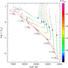 |
Fig. 4. HR diagram of solar metallicity models without (dashed black line) and with rotation (solid coloured lines; here we show the fast rotators). The values of the surface velocity normalised to the break-up value (Ω/Ωcrit) increase from blue to red as shown on the right colour bar. The black triangles indicate when the rotating models are released from their disc. The red lines indicate the standard (dashed) and rotating (solid) ZAMS. |
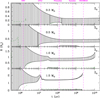 |
Fig. 5. Kippenhahn diagram showing the evolution of the internal structure of the non-rotating solar metallicity models of 0.3 (top), 0.5, 1.0 and 1.5 M⊙ (bottom) from the PMS up to the end of the main sequence. The upper line represents the surface radius and hatched areas refer to convective regions. The green line displays the H-burning limit. The five pink vertical lines indicate the ages of open clusters used as markers of the evolution. |
For the mass range considered in the present grid, this effect is only relevant for the fast-rotating models. The median and slow rotators follow the same evolutionary path in the HR diagram as their standard counterparts. This shift towards lower temperatures in the evolutionary tracks of fast rotators is visible at different locations on the PMS and MS depending on the initial mass (1) at the tip of the Hayashi line in the HR diagram (red part of the tracks in Fig. 4) where the model stars are initially very extended and contracting very rapidly; (2) at the end of the PMS for models more massive than 0.6 M⊙ that undergo a final contraction after the ignition of core nuclear reactions and before they arrive on the MS; and (3) during the MS evolution for the 1.4 and 1.5 M⊙ models.
As can be seen in Fig. 4, the ZAMS of the fast rotators is reached at cooler temperatures due to the effects of the centrifugal acceleration, and this shift increases with initial mass5. The lower the initial mass, the closer to the standard location of the ZAMS. Below 0.6 M⊙ the ratio Ω/Ωcrit never exceeds 0.4 after the star is decoupled from its disc (indicated with black triangles in Fig. 4). The deformation of the stellar structure by centrifugal forces is negligible, and the rotating tracks on the HR diagram follow the standard tracks.
Between 0.6 M⊙ and 1.3 M⊙ at solar metallicity, the models reach fairly high rotation rates on their arrival on the ZAMS (up to 0.9Ωcrit), and in the HR diagram they thus appear much cooler. However, owing to their thick convective envelope, they are efficiently spun down, and converge towards the standard non-rotating tracks on the MS. On the early MS, while the star is almost still in the HR diagram, its surface velocity can change substantially (e.g. Barnes et al. 2016). For example, it takes 2 × 10⁸ years for a fast-rotating 1 M⊙ model to spin down from 75% to less than 10% of the critical velocity, while in the same amount of time the luminosity increases by only 1–2% and less than 2% of the hydrogen has been burnt in the core. This rapid spin-down leads to an increase in the effective temperature at almost constant luminosity from the fast-rotating cooler ZAMS to the slow-rotating hotter MS.
The 1.4 and 1.5 M⊙ models have a very thin convective envelope on the MS, and hence lose almost no AM through magnetic braking. They maintain a high Ω/Ωcrit value during most of the MS, so their evolutionary tracks in the HRD remain cooler than the standard ones.
5.2. Evolution of surface rotation on the PMS and MS
The evolution of the surface rotation of low-mass stars during the PMS and MS is due to the combined effects of the structural changes, the efficiency of the torque exerted by magnetised winds at the stellar surface, and the internal transport of AM. Figure 6 presents the evolution of the surface angular velocity of the fast- (left), median- (centre), and slow- (right) rotating models of all masses at solar metallicity.
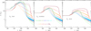 |
Fig. 6. Evolution of surface angular velocity as a function of time at Z = Z⊙ for fast (left), median (centre) and slow (right) rotators from 0.4 M⊙ (neon green) up to 1.5 M⊙ (burgundy), the 0.2 and 0.3 M⊙ are shown in black short- and long-dashed lines, respectively. |
On the PMS, as long as the star is coupled to its disc, i.e. its angular velocity is kept constant in the model, the break-up velocity increases when the star contracts. The ratio Ω/Ωcrit thus decreases over this period so all the rotating models progressively join their standard tracks (see Fig. 4).
After the star–disc decoupling the stars are free to spin up, and they reach a maximum velocity that is higher for higher stellar mass. This surface acceleration is driven by the structural changes. In the case of the initially fast rotators, the most massive models can even reach close to break-up surface velocities as they approach the ZAMS (red part of the tracks on Fig. 4).
All the models with masses below 1.4 M⊙ (at Z⊙) reach their maximum velocity at their arrival on the ZAMS and then spin down on the MS when magnetic braking kicks in (see Fig. 6). This peak velocity coincides with the onset of core convection following the activation of the 12C(p, γ) reaction that stops the star’s contraction. The fully convective 0.2 and 0.3 M⊙ models start spinning down when the contraction rate has slowed down and the magnetised wind torque has strengthened (around 108 yr for the 0.3 M⊙).
In the fastest rotators the magnetic field is saturated (Ro < 0.14) when the effect of the stellar wind torque first becomes effective, and then switches to the unsaturated regime as the surface angular velocity decreases. The early MS evolution of the surface velocity of all fast rotators thus starts with a rapid spin-down followed by a more progressive decrease in the spin rate. This transition between the saturated and unsaturated regime is indicated in Fig. 6 by the change in the slope. We also notice that in the unsaturated regime the spin velocity follows a Skumanich-like relation with Ω ∝ t−p. Finally, the slow and median rotators with masses (M ≥ 0.9 M⊙) and the fast rotators with M ≥ 1.3 M⊙ always evolve in the unsaturated regime.
The magnetic braking as included in our models, however, proves to be inefficient for the most massive models (≥1.4 M⊙). These stars have a very thin convective envelope with a high convective turnover timescale (i.e. a high Rossby number) on the MS (see Fig. 5), and hence lose almost no AM through magnetic torques. The observations also become very sparse in this mass range due to the lack of surface magnetic spots in these stars, which are needed to consistently retrieve the rotation period from photometry.
In their late evolution, the surface velocities of models with the same initial mass but different initial rotation rates converge to the same value, so no constraints can be obtained on the initial AM content of stars based on their MS rotation rate (see also Kawaler 1988; Amard et al. 2016). The overall behaviour described above is compatible with the observational results by Folsom et al. (2016, 2018) who showed that the evolution of the magnetic field strength and of its geometry, which define the torque applied at the stellar surface, are primarily driven by structural changes during the PMS, while on the MS they correlate with the angular velocity of the star.
5.3. Surface rotation: comparison to observations
In Amard et al. (2016), we compared the surface angular velocity evolution predicted by the 1 M⊙ models at Z⊙ to rotation periods measurements of solar-type stars in star forming regions and young open clusters (1 Myr–2.5 Gyr). The models were computed with different physical descriptions for the internal transport and extraction of AM. We found an overall good agreement between the predicted and observed surface rotation rate, with the models presenting a relatively strong differential rotation profile along most of the evolution. We concluded that the rotational evolution of young stars is insufficient to constrain the internal transport of AM.
In this section, we extend this comparison to a broader range of stellar masses for models with updated input physics. We focus on solar metallicity where more data are available, which allows us to cover a wider range of ages. We recall that each grid, characterised by its metallicity and initial angular velocity Ωinit, is computed with the same value for the disc-coupling timescale (τDL) independently of the initial stellar mass and metallicity (except for the fast-rotating models with M ∈ [1.2−1.5] M⊙; see Table 3 and Sect. 2.6.3). Figure 7 shows a comparison of the surface rotation periods predicted by our solar metallicity grid to the observed rotation periods of open clusters members, at the age given in the literature for each cluster. The overall shape and evolution of the observed rotation period as a function of mass is nicely reproduced by our models. Here we summarise the main observational points and compare them to model predictions.
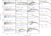 |
Fig. 7. Comparison over the whole mass range, between 0.2 and 1.5 M⊙, of the rotation period distributions of our solar metallicity models with observations from open clusters of increasing ages (grey crosses, data from Gallet & Bouvier 2013; Bouvier et al. 2014; Douglas et al. 2016, 2017; Agüeros et al. 2018). The red, green, and blue crosses represent the rotation periods of the slow-, median-, and fast-rotating grids, respectively. Masses and ages of cluster members are taken from the literature. |
-
During the first few million years the rotation period presents a large dispersion (ΔProt ≈ 10 days) that remains roughly constant (see e.g. ONC, NGC 6530, NGC 2254, CepOB3b, and NGC 2362, first column of Fig. 7). Nonetheless, Somers et al. (2017) mention the presence in young clusters of a correlation between the stellar mass and the rotation period, with the less massive stars having the shortest period. This may indicate that the less massive stars are already spinning up and therefore could have shorter disc lifetimes. We did not account for this feature, but despite this limitation our models still remain in fair agreement with observations at these very early ages.
-
The second phase (second column of Fig. 7) corresponds to the time when the PMS stars are released from their disc and are free to spin up. For clusters covering this period (a few 106 yr), the dichotomy between fast and slow rotator sequences is very clear, as exemplified by hPer (13 Myr). Some observed stars are very close to the break-up velocity, and they are not expected to have ended their contraction yet. With our adopted initial conditions, we are able to reproduce most of the spread in rotation period in hPer and the two sequences running along the red and blue crosses observed in pre-ZAMS clusters.
-
By the age of the Pleiades (125 Myr) the models above 1.2 M⊙ have been efficiently braked and the initially slow and fast rotators start to merge into a unique sequence. This is not the case for the lower mass models that evolve more slowly and may still be contracting.
-
In the third column of Fig. 7, we see a variation in the observed dispersions of slow rotators with mass and age. Stars with a lower mass reach this sequence later than their more massive counterparts because the contraction phase lasts longer, and because the magnetic field saturates for a lower rotation rate they enter a regime of saturated magnetic field for a longer time, which delays their spin-down. The models are also able to reproduce the progressive convergence of the slow (red) and fast (blue) sequences. At the age of Praesepe (580 Myr), the fit to the observed dispersion is very good down to 0.4 M⊙, but the models fail to reproduce the short rotation period of the less massive stars. This discrepancy between model predictions and observations is discussed in Agüeros et al. (2018) and appears at the mass transition where the star remains fully convective. For these very low-mass stars, our braking prescription is too efficient and/or happens too early. This indicates that the expression and calibration of the braking law should be modified in this low-mass fully convective regime (e.g. Matt et al. 2015).
-
We then reach the fourth column where the data can be used for gyrochronology. By 1 Gyr, all stars have spun down. Our models can reproduce fairly closely the evolution of the rotational velocity of solar-type stars, but they fail to account for the relatively flat distribution of periods over the entire mass range. Above 1.2 M⊙, the predicted rotational period is too short compared to the observations, and at smaller masses the discrepancy is not as severe but our models slightly overestimate the spin rate. We note that above 1.2 M⊙, main-sequence stars have a thinner convective envelope than their lower mass counterparts and also develop a convective core during central H-burning. The structure of the dynamo-generated magnetic field may change with the size of the convective envelope, going from a dominant dipolar large-scale component to a more multipolar field organised on smaller scales (Donati 2011). This would surely affect the braking efficiency, even if it is not clear whether such an evolution would explain the observed discrepancy. A field organised as a higher degree multipole is expected to have a weaker lever arm, and hence reduce AM loss (e.g. Réville et al. 2015; Finley & Matt 2018; See et al. 2018; Garraffo et al. 2018), which is opposite to what appears to be needed to reconcile our models with observations. We finally note that the 0.4 and 0.5 M⊙ models spin too slowly compared to the observed rotation periods in NGC 6819. It likely comes from the incomplete transport of AM and the corresponding calibration constant (K) that we selected for the 1.0 M⊙ models. These stars are on the verge of the fully convective mass domain and have a very deep convective envelope, thus they rotate nearly as solid bodies (since we assumed constant angular velocity in convective regions). For example, if we had considered a solid body for the Sun, the calibration constant would have been smaller, resulting in a smaller torque and a larger angular velocity at later ages (see also Amard et al. 2016 for discussion on the impact of the constant K).
5.3.1. Cluster age uncertainties
The cluster ages reported in Fig. 7 are taken from the literature6, and the masses for the sample stars are from Gallet & Bouvier (2013), Bouvier et al. (2014), Douglas et al. (2016, 2017), Agüeros et al. (2018), and references therein. The ages of the youngest clusters (up to hPer) are relatively uncertain, sometimes a factor of two uncertainty depending on the sets of isochrones used to fit their colour-magnitude diagram (CMD). One of the main reasons for this uncertainty is the poor radius determination of very low-mass and very cool dwarf models. Eclipsing low-mass binaries exhibit inflated radii in comparison to those provided by any evolutionary models, which impacts their location in the HR diagram (see e.g. Baraffe et al. 2015). Bell et al. (2013) provided empirical corrections to theoretical isochrones in order to better reproduce the colour–magnitude diagram in all colours. These corrections give ages up to a factor of 2 greater than those obtained with standard isochrones. However, a caveat of these corrections is that, except for the age, all the parameters of the corresponding evolutionary models are no longer consistent. Somers & Pinsonneault (2015) proposed that stars populating the youngest open clusters are strongly magnetised and would develop a high activity level leading to a high spot coverage. These cool spots on the surface would then induce a back-reaction on the structure and the star would puff up and mimic the expected inflated radius. Finally, Feiden & Chaboyer (2012) have provided some evolutionary models including a simplified treatment of the effects of magnetic field on the structure. This formalism leads to a less efficient convection that inflates the stellar radius and reproduces fairly well the CMD of young open clusters, but requires very strong magnetic fields.
5.4. Internal rotation: effect of initial mass
Figure 8 shows the level of internal differential rotation ΔΩ for the slow and fast rotators of all solar metallicity models7 as a function of time from the onset of the radiative core to the TAMS (or up to 15 Gyr for the models that have a longer MS lifetime). We express it as
 (20)
(20)
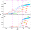 |
Fig. 8. Differential rotation as a function of time for slow (top) and fast (bottom) rotators at Z = Z⊙. The colour-coding is the same as in Fig. 6. |
where MCZ is the mass coordinate at the base of the convective envelope and ΩS the surface angular velocity. With this formulation ΔΩ → −1 corresponds to a slow-rotating core with a fast-rotating envelope, ΔΩ = 0 corresponds to a flattened rotation profile on average, and ΔΩ = 1 is characteristic of a fast-rotating core with a slowly rotating surface. We note that ΩC is not comparable to the solar core value derived by helioseismology, as in e.g. Fossat et al. (2017) where they claim that the solar core is rotating five times faster than the solar surface. According to our unit system, ΔΩ⊙ = 0.12 (see Fig. 10). As seen in Fig. 8, all our models evolve between these last two cases, namely ΔΩ = 0 and ΔΩ = 1.
During the PMS phase, the contraction of the star and then the appearance of the convective core (when it exists) generate a strong meridional circulation, which remains the main driver for AM transport. Meridional circulation in these models only transports AM from the core to the surface. This is in agreement with our previous study of solar-mass, solar metallicity stars in Amard et al. (2016). The efficiency of the circulation depends directly on the rotation rate. Therefore, the more rapidly the star is spinning, the closer to solid body it is. This is valid for all the stellar masses we consider here.
In slow-rotating models, ΔΩ increases while the radiative core appears during the PMS, as shown in the top panel of Fig. 8. Its value rises from 0 at the age of the ONC (the fully convective star is in solid-body rotation), up to ΔΩ = 0.7 at the age of the Hyades for the 0.5 M⊙ model and ΔΩ = 0.4 at the age of hPer for the slow-rotating 1.4 M⊙ model. This strong differential rotation results almost exclusively from the structural changes (stellar contraction and shrinkage of the convective envelope) because at that stage the rotation rate is slow and the internal AM transport by meridional circulation and shear turbulence is negligible.
Then on the MS we can distinguish two families of slow rotators. Models with Mini > 1.2 M⊙ have a thin convective envelope (see Fig. 5) characterised by a short convective turnover timescale so, for a given rotation rate they are associated with a high Rossby number (see Sect. 5.6). They are thus expected to have a less active dynamo, and the torque applied at their surface is reduced. This implies that more massive models can maintain a high rotation rate during their main sequence evolution which in turn can trigger stronger meridional currents capable of reducing the degree of differential rotation.
For stars with Mini < 1.2 M⊙ the differential rotation increases with time because they have more extended CE and can generate stronger magnetic torques. Their surface spin rate is thus lower and angular momentum transport redistribution in the radiative interior less efficient. A situation is thus reached in which the differential rotation rate keeps slowly increasing due to the surface braking and the negligible effect of meridional currents.
The fast rotators present a very different behaviour. They strongly couple the radiative core to the convective envelope for a longer period of time, which extends beyond 108 yr. They have very strong meridional currents that carry AM from the radiative core to the convective envelope and reduce the differential rotation, as discussed for the 1 M⊙ case in Amard et al. (2016). When the stars are sufficiently spun down by the magnetised stellar wind, the surface angular velocity decreases, and differential rotation develops below the convective envelope where a nearly flat rotational profile was established during the fast-rotating phase. If the convective envelope is too small to ensure efficient braking, a flat rotation profile is maintained as can be seen for the 1.4–1.5 M⊙ models. For these last two models, the sudden rise in ΔΩ at the very end of the MS is due to the deepening of the surface convection zone.
In Fig. 9, the rotation profiles at the ZAMS of the median-rotating models present a minimum surface angular velocity around 0.6 M⊙ (short dashed olive green track). This is also observed with the slow and fast rotators around the same mass. Above this limit, the stars are braked less efficiently due to a smaller convective envelope, while below this limit, stars have been contracting efficiently towards the ZAMS, maintaining a higher surface rotation rate.
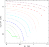 |
Fig. 9. Angular velocity profile as a function of the relative mass fraction of the median-rotating models at solar metallicity for the 0.4–1.5 M⊙ mass range on the ZAMS. The colour-coding is the same as in Fig. 6. |
To date, there are very few main-sequence low-mass stars for which estimates of the core angular velocity is accessible through asteroseismic analysis. Benomar et al. (2015) published a sample of 22 F stars with surface (envelope) and core rotation rates. We selected half of their sample, keeping those with [Fe/H] = ±0.1 for which we computed ΔΩ assuming a solid-body rotating radiative core, which is debatable. Figure 10 shows the obtained values as a function of effective temperature together with our solar metallicity models of equivalent masses. The solar value deduced from the controversial Fossat et al. (2017) rotation profile (see Schunker et al. 2018) is also represented in this plot. The 1.4 and 1.5 M⊙ models have a degree of differential rotation close to what is given by asteroseismology for Teff > 6300 K. However, our models fail to reproduce lower temperature data as our formalism does not produce any reversed rotation profiles, i.e. with a core that rotates more slowly than the surface. Internal gravity waves (IGWs) have been shown to produce this type of rotation profile and start to operate in this temperature range (e.g. Charbonnel et al. 2013). A more in-depth study on that topic would therefore be a natural extension to this preliminary work. We also note that in our solar-mass model, the coupling between the radiative interior and convective envelope is too weak to match the solar value derived from the Fossat et al. (2017) data. A stronger coupling could be achieved, however, by the action of IGWs (e.g. Charbonnel & Talon 2005). We note here that despite this discrepancy, our models are able to reproduce the only sound observational constraint available on the rotation of low-mass stars, which is given by the evolution of their surface rotation period.
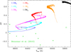 |
Fig. 10. Differential rotation (ΔΩ) as a function of effective temperature for our solar metallicity 1.0–1.5 M⊙ models with a median initial rotation rate. Green diamonds show the value of ΔΩ from the Benomar et al. (2015) data. The solar value as given by Fossat et al. (2017) is indicated by ⊙. |
5.5. Impact of metallicity on rotation
The structure of a star depends on its mass, but also on its chemical composition as illustrated in Fig. 11 showing the Kippenhahn diagram of a non-rotating 1.3 M⊙ model at three different metallicities.
For a given mass, a lower metal content reduces the global opacity, making the star hotter, more compact, and with a thinner convective envelope. So for AM evolution, a lower metallicity generates a weaker torque so a larger surface velocity can be reached. Reciprocally, a higher metal content produces slower rotators. Additionally, and as can be seen in Fig. 11, stars that are more metal-poor contract on a shorter timescale and their radiative core develops earlier on the PMS. Hence, they spin up more rapidly and reach the less efficient braking (saturated) regime earlier.
In the top panel of Fig. 12, we show the surface rotation rate for three masses, five metallicities, and two initial velocities corresponding to the fast and slow rotators. The models with Z = 0.0059 ([Fe/H] = −0.5 in blue) or Z = 0.0022 ([Fe/H] = −1.0 in magenta) spin up faster than those with a solar or higher metal content (Z = 0.0134 or Z = 0.026 ([Fe/H] = +0.3)) and remains on the MS with faster surface rotation rates. The main difference is the transition to the unsaturated regime that is reached at higher velocities for lower metallicity models. For example, in the fast-rotating 1 M⊙ case, the most metal-poor models saturate around 30 Ω⊙, while the solar metallicity models saturate at only 6 Ω⊙. Then in the unsaturated regime, the models converge to the same Ω ∝ t−p relation, independently of the metallicity.
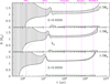 |
Fig. 11. Kippenhahn diagram of a standard 1.3 M⊙ models at three metallicities: Z = 0.02564 (top), Z⊙ (middle), and Z = 0.0059 (bottom) from the PMS to the end of the main sequence. The legend is the same as in Fig. 5. |
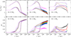 |
Fig. 12. Top: evolution of the surface rotation rate for three different masses at five metallicities, Z = 0.0022 (magenta), Z = 0.0059 (blue), Z = 0.0079 (green), Z = 0.0134 (red), and Z = 0.0256 (black) for the fast (dash-dotted) and slow (solid) rotating cases. Bottom: evolution of the relative differential rotation rate ΔΩ using the same colour-coding as before. |
Regarding the internal rotation properties, a metal-poor star has a more extended radiative region at a given evolutionary point on the MS, thus according to Eqs. (5) and (6), the meridional circulation and shear turbulence AM flux are both enhanced, leading to less differential rotation. This configuration favours solid-body rotation in metal-poor stars. This is illustrated in the bottom panel of Fig. 12 showing the evolution of ΔΩ as given by Eq. (20). For the three considered masses, the degree of differential rotation on the main sequence is always smaller for lower metallicity models. The result is especially clear in the case of the 1.3 M⊙ model, for which the evolution of the rotation velocity on the main sequence is strongly metal dependent.
Therefore, given an initial mass and rotational period, a lower metallicity model will reach a higher surface angular velocity and have less internal differential rotation. As a word of caution, this result may only be an artefact caused by one of our assumptions, namely that we consider the same disc-coupling timescale independently of the initial mass and metallicity.
Many factors affect the physics of the disc. It is not clear yet if the photo-evaporation mechanism, accretion-related processes, or a combination of planet formation mechanism and photo-evaporation is dominant in the disc dispersal process (e.g. Alexander et al. 2014; Gorti et al. 2015). The in situ planet formation process is now known to open large gaps in protoplanetary discs (Brogan & Pérez 2015) that could contribute to a more efficient disc dispersal by photo-evaporation (Alexander 2014). On the one hand, if the photo-evaporation mechanism is dominant, the higher luminosity of a metal-poor star should provoke a quicker disc dispersal. On the other hand, metallicity is a direct indicator of the condensible materials available in the disc to form planets. Planetary system formation simulations by Dawson et al. (2015) and observations from the Kepler mission show a larger fraction of large planets in metal-rich environments (e.g. Narang et al. 2018; Cabral et al. 2019). Mamajek (2009) and Mulders (2018) suggest that metal-rich stars would lose their discs earlier because of planet formation.
5.6. Rossby numbers
The efficiency of the dynamo process that is expected to be responsible for the stellar magnetic field can be characterised by the Rossby number defined in Eq. (10). The lower the Rossby number, the more active the dynamo engine, until the magnetic field eventually saturates. Given the wide range of convective envelope scales (in mass and radial extent), the depth at which the turnover timescale is computed is particularly relevant. Charbonnel et al. (2017) explored this parameter space and proposed several options that we provide at the CDS as described in Table A.1.
We show in Fig. 13 the evolution of the Rossby number for median rotators with three different initial masses at solar metallicity compared to semi-empirical values of solar-like stars taken from the literature. In the present case, we compute the Rossby number according to Eq. (10), with the characteristic turnover timescale taken at half a pressure scale height above the base of the convective envelope. The Rossby number sharply drops when the radiative core appears before increasing more slowly as the envelope becomes thinner. Subsequently, the spin-down due to magnetic winds explains the increase in the Rossby number, up to the end of the MS. Also, the lower the stellar mass, the smaller the Rossby number, due to the more extended convective envelope.
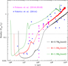 |
Fig. 13. Rossby number as a function of time for the 0.7 (black), 1.0 (red), and 1.3 (green) M⊙ models for median rotators. The Rossby number is estimated at half a pressure scale height above the base of the convective envelope. The dotted line indicates the saturation Rossby number at Ro = 0.14. The blue and magenta triangles indicates the semi-empirical Rossby numbers for solar-like stars given in Folsom et al. (2016, 2018) and Vidotto et al. (2014b). |
As in Charbonnel et al. (2017), we compared our models to semi-empirical Rossby numbers taken from observational studies. We selected the observations by Folsom et al. (2016, 2018) carried out as part of the ToUpiES8 project, and the compilation by Vidotto et al. (2014b). They use spectro-polarimetric data to study the evolution of magnetic field with rotation and time and provide Rossby numbers that they estimated using different methods. We selected the stars with M ∈ [0.7; 1.3] M⊙ in the two samples, and as can be seen in Fig. 13, our median rotators are in good agreement with both of their samples on the PMS and the MS.
5.7. Lithium surface abundance
As we mention in the introduction, rotation induced mixing processes associated with meridional circulation and shear-induced mixing cannot explain by themselves the 7Li abundances observed in open clusters. Classically, the higher the differential rotation in the tachocline9, the more efficient the mixing and the more important the depletion of 7Li. In the present case, our 1 M⊙ models (Fig. 14) cannot reproduce the observed main-sequence lithium depletion observed for t > 109 yr. Additional processes including extra mixing in the tachocline (see e.g. Brun et al. 1999; Christensen-Dalsgaard et al. 2018) or internal gravity waves (e.g. Charbonnel & Talon 2005) are required to account for this feature.
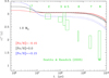 |
Fig. 14. Evolution of the 7Li surface abundance for our rotating 1 M⊙ models at different metallicities. The solid, dotted, and dashed lines refer to the fast-, median-, and slow-rotating case, respectively. We overplotted the spectroscopic 7Li abundances observed in some open clusters and collected by Sestito & Randich (2005). The numbers 1 to 8 identify the clusters: (1) NGC 2264; (2) IC 2391, IC 2602, and IC 4665; (3) Pleiades and Blanco I; (4) NGC 2516; (5) M 34, M 35, and NGC 6475; (6) Hyades, Praesepe, Coma Ber, and NGC 6633; (7) NGC 752, NGC 36780, and IC 4651; and (8) M 67. The solar abundance is indicated with ⊙. |
6. Conclusions
The present work can be considered as an update of the grid of PMS models and isochrones by Siess et al. (2000). We presented the first grid of stellar models of low-mass PMS and MS stars including a self-consistent treatment of the effects of rotation. The grid extends from 0.2 M⊙ up to 1.5 M⊙ for seven metallicities and includes state-of-the-art micro- and macro-physics with improved surface boundary conditions and the current treatment of anisotropic turbulence (Mathis et al. 2018). Our standard solar metallicity models are thoroughly compared with a large set of available evolutionary tracks, and except for differences on the MS for very low-mass stars related to the equation of state, they show good agreement over the whole evolution. However, significant differences in terms of age and evolutionary timescale appear between different grids and are likely due to a complex interplay between the physical grid assumptions and the numerics of each code. After calibration of the solar rotation with three parameters for the braking law and none for the internal transport, the models are able to reproduce fairly well the evolution of the surface rotation rate observed in associations and open clusters at solar metallicity over the entire mass range 0.2–1.5 M⊙. However, they still fail to account for the observed main-sequence lithium depletion observed in the more evolved open clusters. We also confronted our models to asteroseismic data probing the core rotation rate. We found good agreement between our mid-F-type star models and the observations, but below ≈1 M⊙, our models can no longer explain the slow core rotation rates claimed by Benomar et al. (2015). Finally, we compared our model predictions to semi-empirical Rossby number determinations and found a very good agreement. We also showed that metallicity has a strong impact on the AM losses and on the rotation period evolution of low-mass stars. Metal-poor stars spin faster than metal-rich ones. We provide extended tables describing the evolution of key stellar parameters, including asterosesismic quantities and Rossby numbers. The data are available on the Geneva website10. They are integrated in the SYCLIST tool allowing the computation of isochrones and synthetic clusters (Georgy et al. 2014).
The computation at different metallicities offers the possibility to compare the grid to new incoming data. Among other missions (for example TESS or PLATO), Gaia is expected to provide rotation periods and spectroscopic data for a few million stars. This can be a fantastic laboratory and a great opportunity to test the robustness of rotational treatment for different chemical compositions.
We arbitrarily define the ZAMS as the time when 0.2% of the initial hydrogen has been burnt at the centre.
The ZAMS of the massive rotating models moves closer to the standard location due to the lower initial angular velocity assumed for the fast-rotating 1.3 to 1.5 M⊙ models.
We plan to redetermine the cluster ages with our own isochrones in a future paper.
The 0.2 M⊙ and 0.3 M⊙ models are not presented as they evolve as fully convective stars.
The tachocline is the transition region between the radiative interior and the convective envelope.
Acknowledgments
This study was supported by the grant ANR 2011 Blanc SIMI5-6 020 01 “Toupies: Towards understanding the spin evolution of stars” (http://ipag.osug.fr/Anr_Toupies/). LA thanks the European Research Council for their support through the grant ERC 682393 (AWESoMeStars). CC, LA, FG, and CG thank the Equal Opportunity Office of the University of Geneva. LA, AP, CC, FG, and NL thank the Programme National de Physique Stellaire (PNPS) of CNRS/INSU co-funded by CEA and CNES for their financial support. FG acknowledges financial support from the CNES fellowship. LS is a senior FNRS research associate.
References
- Adelberger, E. G., Austin, S. M., Bahcall, J. N., et al. 1998, Rev. Mod. Phys., 70, 1265 [NASA ADS] [CrossRef] [Google Scholar]
- Agüeros, M. A., Bowsher, E. C., Bochanski, J. J., et al. 2018, ApJ, 862, 33 [NASA ADS] [CrossRef] [Google Scholar]
- Alexander, R. 2014, in Exploring the Formation and Evolution of Planetary Systems, eds. M. Booth, B. C. Matthews, & J. R. Graham, IAU Symp., 299, 179 [NASA ADS] [Google Scholar]
- Alexander, D. R., & Ferguson, J. W. 1994, ApJ, 437, 879 [NASA ADS] [CrossRef] [Google Scholar]
- Alexander, R., Pascucci, I., Andrews, S., Armitage, P., & Cieza, L. 2014, Protostars and Planets VI, 475 [Google Scholar]
- Allard, F., Homeier, D., & Freytag, B. 2011, in 16th Cambridge Workshop on Cool Stars, Stellar Systems and the Sun, eds. C. Johns-Krull, M. K. Browning, & A. A. West, ASP Conf. Ser., 448, 91 [NASA ADS] [Google Scholar]
- Allard, F., Homeier, D., & Freytag, B. 2012, in IAU Symp., eds. M. T. Richards, & I. Hubeny, 282, 235 [NASA ADS] [Google Scholar]
- ALMA Partnership, Brogan, C. L., Pérez, L. M., et al. 2015, ApJ, 808, L3 [NASA ADS] [CrossRef] [Google Scholar]
- Amard, L., Palacios, A., Charbonnel, C., Gallet, F., & Bouvier, J. 2016, A&A, 587, A105 [NASA ADS] [CrossRef] [EDP Sciences] [Google Scholar]
- Asplund, M., Grevesse, N., & Sauval, A. J. 2005, in Cosmic Abundances as Records of Stellar Evolution and Nucleosynthesis, eds. T. G. Barnes III, & F. N. Bash, ASP Conf. Ser., 336, 25 [NASA ADS] [Google Scholar]
- Asplund, M., Grevesse, N., Sauval, A. J., & Scott, P. 2009, ARA&A, 47, 481 [NASA ADS] [CrossRef] [Google Scholar]
- Bahcall, J. N., & Pinsonneault, M. H. 1992, ApJ, 395, L119 [NASA ADS] [CrossRef] [Google Scholar]
- Ballot, J., García, R. A., & Lambert, P. 2006, MNRAS, 369, 1281 [NASA ADS] [CrossRef] [Google Scholar]
- Baraffe, I., Chabrier, G., Allard, F., & Hauschildt, P. 1998, VizieR Online Data Catalog: J/A+A/333/403 [Google Scholar]
- Baraffe, I., Homeier, D., Allard, F., & Chabrier, G. 2015, A&A, 577, A42 [NASA ADS] [CrossRef] [EDP Sciences] [Google Scholar]
- Barnes, S. A., Spada, F., & Weingrill, J. 2016, Astron. Nachr., 337, 810 [NASA ADS] [CrossRef] [Google Scholar]
- Belkacem, K., Marques, J. P., Goupil, M. J., et al. 2015, A&A, 579, A31 [NASA ADS] [CrossRef] [EDP Sciences] [Google Scholar]
- Bell, C. P. M., Naylor, T., Mayne, N. J., Jeffries, R. D., & Littlefair, S. P. 2013, MNRAS, 434, 806 [NASA ADS] [CrossRef] [Google Scholar]
- Bemmerer, D., Confortola, F., Costantini, H., et al. 2006, Phys. Rev. Lett., 97, 122502 [NASA ADS] [CrossRef] [PubMed] [Google Scholar]
- Benomar, O., Takata, M., Shibahashi, H., Ceillier, T., & García, R. A. 2015, MNRAS, 452, 2654 [NASA ADS] [CrossRef] [Google Scholar]
- Borucki, W. J., Koch, D., Basri, G., et al. 2010, Science, 327, 977 [NASA ADS] [CrossRef] [PubMed] [Google Scholar]
- Bouabid, M.-P., Dupret, M.-A., Salmon, S., et al. 2013, MNRAS, 429, 2500 [NASA ADS] [CrossRef] [Google Scholar]
- Bouvier, J., Matt, S. P., Mohanty, S., et al. 2014, Protostars and Planets VI, 433 [Google Scholar]
- Bressan, A., Marigo, P., Girardi, L., et al. 2012, MNRAS, 427, 127 [NASA ADS] [CrossRef] [Google Scholar]
- Brott, I., & Hauschildt, P. H. 2005, in The Three-Dimensional Universe with Gaia, eds. C. Turon, K. S. O’Flaherty, & M. A. C. Perryman, ESA Spec. Publ., 576, 565 [NASA ADS] [Google Scholar]
- Brun, A. S., & Browning, M. K. 2017, Liv. Rev. Sol. Phys., 14, 4 [Google Scholar]
- Brun, A. S., Turck-Chièze, S., & Zahn, J. P. 1999, ApJ, 525, 1032 [NASA ADS] [CrossRef] [Google Scholar]
- Cabral, N., Lagarde, N., Reylé, C., Guilbert-Lepoutre, A., & Robin, A. 2019, A&A, 622, A49 [Google Scholar]
- Caffau, E., Maiorca, E., Bonifacio, P., et al. 2009, A&A, 498, 877 [NASA ADS] [CrossRef] [EDP Sciences] [Google Scholar]
- Caffau, E., Ludwig, H.-G., Steffen, M., Freytag, B., & Bonifacio, P. 2011, Sol. Phys., 268, 255 [NASA ADS] [CrossRef] [Google Scholar]
- Cantiello, M., Mankovich, C., Bildsten, L., Christensen-Dalsgaard, J., & Paxton, B. 2014, ApJ, 788, 93 [Google Scholar]
- Caughlan, G. R., & Fowler, W. A. 1988, Atomic Data and Nuclear Data Tables, 40, 283 [Google Scholar]
- Ceillier, T., Eggenberger, P., García, R. A., & Mathis, S. 2012, Astron. Nachr., 333, 971 [NASA ADS] [CrossRef] [Google Scholar]
- Chaboyer, B., & Kim, Y.-C. 1995, ApJ, 454, 767 [NASA ADS] [CrossRef] [Google Scholar]
- Chaboyer, B., & Zahn, J.-P. 1992, A&A, 253, 173 [Google Scholar]
- Chantereau, W., Charbonnel, C., & Decressin, T. 2015, A&A, 578, A117 [NASA ADS] [CrossRef] [EDP Sciences] [Google Scholar]
- Charbonnel, C., & Talon, S. 2005, Science, 309, 2189 [Google Scholar]
- Charbonnel, C., Decressin, T., Amard, L., Palacios, A., & Talon, S. 2013, A&A, 554, A40 [NASA ADS] [CrossRef] [EDP Sciences] [Google Scholar]
- Charbonnel, C., Decressin, T., Lagarde, N., et al. 2017, A&A, 605, A102 [NASA ADS] [CrossRef] [EDP Sciences] [Google Scholar]
- Chen, Y., Girardi, L., Bressan, A., et al. 2014, MNRAS, 444, 2525 [NASA ADS] [CrossRef] [Google Scholar]
- Choi, J., Dotter, A., Conroy, C., et al. 2016, ApJ, 823, 102 [NASA ADS] [CrossRef] [Google Scholar]
- Christensen-Dalsgaard, J., Gough, D. O., & Knudstrup, E. 2018, MNRAS, 477, 3845 [NASA ADS] [CrossRef] [Google Scholar]
- Coc, A., Vangioni-Flam, E., Descouvemont, P., Adahchour, A., & Angulo, C. 2004, ApJ, 600, 544 [NASA ADS] [CrossRef] [Google Scholar]
- Cranmer, S. R., & Saar, S. H. 2011, ApJ, 741, 54 [NASA ADS] [CrossRef] [Google Scholar]
- Cyburt, R. H., Amthor, A. M., Ferguson, R., et al. 2010, ApJS, 189, 240 [NASA ADS] [CrossRef] [Google Scholar]
- Dawson, R. I., Chiang, E., & Lee, E. J. 2015, MNRAS, 453, 1471 [NASA ADS] [CrossRef] [Google Scholar]
- Decressin, T., Mathis, S., Palacios, A., et al. 2009, A&A, 495, 271 [NASA ADS] [CrossRef] [EDP Sciences] [Google Scholar]
- Donati, J. F. 2011, in Astrophysical Dynamics: From Stars to Galaxies, eds. N. H. Brummell, A. S. Brun, M. S. Miesch, & Y. Ponty, IAU Symp., 271, 23 [NASA ADS] [Google Scholar]
- Dotter, A., Chaboyer, B., Jevremović, D., et al. 2008, ApJS, 178, 89 [NASA ADS] [CrossRef] [Google Scholar]
- Douglas, S. T., Agüeros, M. A., Covey, K. R., et al. 2016, ApJ, 822, 47 [NASA ADS] [CrossRef] [Google Scholar]
- Douglas, S. T., Agüeros, M. A., Covey, K. R., & Kraus, A. 2017, ApJ, 842, 83 [NASA ADS] [CrossRef] [Google Scholar]
- Eggenberger, P., Maeder, A., & Meynet, G. 2005, A&A, 440, L9 [NASA ADS] [CrossRef] [EDP Sciences] [Google Scholar]
- Eggenberger, P., Meynet, G., Maeder, A., et al. 2010, A&A, 519, A116 [NASA ADS] [CrossRef] [EDP Sciences] [Google Scholar]
- Eggenberger, P., Haemmerlé, L., Meynet, G., & Maeder, A. 2012, A&A, 539, A70 [NASA ADS] [CrossRef] [EDP Sciences] [Google Scholar]
- Ekström, S., Georgy, C., Eggenberger, P., et al. 2012, A&A, 537, A146 [NASA ADS] [CrossRef] [EDP Sciences] [Google Scholar]
- Endal, A. S., & Sofia, S. 1976, ApJ, 210, 184 [NASA ADS] [CrossRef] [Google Scholar]
- Espinosa Lara, F., & Rieutord, M. 2007, A&A, 470, 1013 [NASA ADS] [CrossRef] [EDP Sciences] [Google Scholar]
- Evans, D. W., Riello, M., De Angeli, F., et al. 2018, A&A, 616, A4 [NASA ADS] [CrossRef] [EDP Sciences] [Google Scholar]
- Feiden, G. A., & Chaboyer, B. 2012, ApJ, 757, 42 [NASA ADS] [CrossRef] [Google Scholar]
- Feiden, G. A., Jones, J., & Chaboyer, B. 2015, in Cambridge Workshop on Cool Stars, Stellar Systems, and the Sun, eds. G. T. van Belle, & H. C. Harris, 18, 171 [Google Scholar]
- Ferguson, J. W., Alexander, D. R., Allard, F., et al. 2005, ApJ, 623, 585 [NASA ADS] [CrossRef] [Google Scholar]
- Finley, A. J., & Matt, S. P. 2018, ApJ, 854, 78 [NASA ADS] [CrossRef] [Google Scholar]
- Finley, A. J., Matt, S. P., & See, V. 2018, ApJ, 864, 125 [NASA ADS] [CrossRef] [Google Scholar]
- Folsom, C. P., Petit, P., Bouvier, J., et al. 2016, MNRAS, 457, 580 [NASA ADS] [CrossRef] [Google Scholar]
- Folsom, C. P., Bouvier, J., Petit, P., et al. 2018, MNRAS, 474, 4956 [NASA ADS] [CrossRef] [Google Scholar]
- Forestini, M., & Charbonnel, C. 1997, A&AS, 123, 241 [NASA ADS] [CrossRef] [EDP Sciences] [Google Scholar]
- Fossat, E., Boumier, P., Corbard, T., et al. 2017, A&A, 604, A40 [NASA ADS] [CrossRef] [EDP Sciences] [Google Scholar]
- Fuhrmann, K. 2011, MNRAS, 414, 2893 [NASA ADS] [CrossRef] [Google Scholar]
- Fuller, J., Lecoanet, D., Cantiello, M., & Brown, B. 2014, ApJ, 796, 17 [Google Scholar]
- Gallet, F., & Bouvier, J. 2013, A&A, 556, A36 [NASA ADS] [CrossRef] [EDP Sciences] [Google Scholar]
- Gallet, F., & Bouvier, J. 2015, A&A, 577, A98 [NASA ADS] [CrossRef] [EDP Sciences] [Google Scholar]
- Gallet, F., Charbonnel, C., Amard, L., et al. 2017, A&A, 597, A14 [NASA ADS] [CrossRef] [EDP Sciences] [Google Scholar]
- Garraffo, C., Drake, J. J., Dotter, A., et al. 2018, ApJ, 862, 90 [NASA ADS] [CrossRef] [Google Scholar]
- Georgy, C., Meynet, G., & Maeder, A. 2011, A&A, 527, A52 [NASA ADS] [CrossRef] [EDP Sciences] [Google Scholar]
- Georgy, C., Ekström, S., Granada, A., et al. 2013, A&A, 553, A24 [NASA ADS] [CrossRef] [EDP Sciences] [Google Scholar]
- Georgy, C., Granada, A., Ekström, S., et al. 2014, A&A, 566, A21 [NASA ADS] [CrossRef] [EDP Sciences] [Google Scholar]
- Ghezzi, L., Montet, B. T., & Johnson, J. A. 2018, ApJ, 860, 109 [NASA ADS] [CrossRef] [Google Scholar]
- Ghosh, P., & Lamb, F. K. 1979, ApJ, 234, 296 [NASA ADS] [CrossRef] [Google Scholar]
- Gilliland, R. L., Brown, T. M., Christensen-Dalsgaard, J., et al. 2010, PASP, 122, 131 [NASA ADS] [CrossRef] [Google Scholar]
- Gorti, U., Hollenbach, D., & Dullemond, C. P. 2015, ApJ, 804, 29 [NASA ADS] [CrossRef] [Google Scholar]
- Graboske, H. C., Dewitt, H. E., Grossman, A. S., & Cooper, M. S. 1973, ApJ, 181, 457 [NASA ADS] [CrossRef] [Google Scholar]
- Grevesse, N., & Noels, A. 1993, Phys. Scr. Vol. T, 47, 133 [NASA ADS] [CrossRef] [Google Scholar]
- Grevesse, N., & Sauval, A. J. 1998, Space Sci. Rev., 85, 161 [NASA ADS] [CrossRef] [Google Scholar]
- Hanasoge, S. M., Duvall, T. L., & Sreenivasan, K. R. 2012, Proc. Natl Acad. Sci., 109, 11928 [Google Scholar]
- Hauschildt, P. H., Allard, F., & Baron, E. 1999, ApJ, 512, 377 [NASA ADS] [CrossRef] [Google Scholar]
- Herwig, F. 2000, A&A, 360, 952 [NASA ADS] [Google Scholar]
- Hopf, E. 1930, MNRAS, 90, 287 [NASA ADS] [CrossRef] [Google Scholar]
- Hypolite, D., Mathis, S., & Rieutord, M. 2018, A&A, 610, A35 [NASA ADS] [CrossRef] [EDP Sciences] [Google Scholar]
- Iglesias, C. A., & Rogers, F. J. 1996, ApJ, 464, 943 [NASA ADS] [CrossRef] [Google Scholar]
- Irwin, A. W. 2012, Astrophysics Source Code Library [record ascl:1211.002] [Google Scholar]
- Jermyn, A. S., Tout, C. A., & Chitre, S. M. 2018, MNRAS, 480, 5427 [NASA ADS] [CrossRef] [Google Scholar]
- Johnstone, C. P., Güdel, M., Stökl, A., et al. 2015a, ApJ, 815, L12 [NASA ADS] [CrossRef] [Google Scholar]
- Johnstone, C. P., Güdel, M., Lüftinger, T., Toth, G., & Brott, I. 2015b, A&A, 577, A27 [NASA ADS] [CrossRef] [EDP Sciences] [Google Scholar]
- Johnstone, C. P., Güdel, M., Brott, I., & Lüftinger, T. 2015c, A&A, 577, A28 [NASA ADS] [CrossRef] [EDP Sciences] [Google Scholar]
- Jouve, L., Brown, B. P., & Brun, A. S. 2010, A&A, 509, A32 [NASA ADS] [CrossRef] [EDP Sciences] [Google Scholar]
- Jouve, L., Gastine, T., & Lignières, F. 2015, A&A, 575, A106 [NASA ADS] [CrossRef] [EDP Sciences] [Google Scholar]
- Kawaler, S. D. 1988, ApJ, 333, 236 [NASA ADS] [CrossRef] [Google Scholar]
- Kennedy, G. M., & Kenyon, S. J. 2009, ApJ, 695, 1210 [NASA ADS] [CrossRef] [Google Scholar]
- Krishna Swamy, K. S. 1966, ApJ, 145, 174 [NASA ADS] [CrossRef] [Google Scholar]
- Kurucz, R. L. 1991, Bull. Am. Astron. Soc., 23, 1047 [NASA ADS] [Google Scholar]
- Kurucz, R. L. 1993, SYNTHE Spectrum Synthesis Programs and Line Data (Cambridge: Smithsonian Astrophysical Observatory) [Google Scholar]
- Lagarde, N., Decressin, T., Charbonnel, C., et al. 2012, A&A, 543, A108 [NASA ADS] [CrossRef] [EDP Sciences] [Google Scholar]
- Langer, N. 1998, A&A, 329, 551 [NASA ADS] [Google Scholar]
- Lau, H. H. B., Potter, A. T., & Tout, C. A. 2011, MNRAS, 415, 959 [NASA ADS] [CrossRef] [Google Scholar]
- Li, T. D., Bi, S. L., Yang, W. M., et al. 2014, ApJ, 781, 62 [NASA ADS] [CrossRef] [Google Scholar]
- MacDonald, J., & Mullan, D. J. 2012, MNRAS, 421, 3084 [NASA ADS] [CrossRef] [Google Scholar]
- Maeder, A. 2009, Physics, Formation and Evolution of Rotating Stars (Berlin: Springer Science& Business Media) [Google Scholar]
- Maeder, A., & Meynet, G. 2000, ARA&A, 38, 143 [NASA ADS] [CrossRef] [Google Scholar]
- Maeder, A., & Meynet, G. 2001, A&A, 373, 555 [NASA ADS] [CrossRef] [EDP Sciences] [Google Scholar]
- Maeder, A., & Zahn, J.-P. 1998, A&A, 334, 1000 [NASA ADS] [Google Scholar]
- Mamajek, E. E. 2009, in AIP Conf. Ser., eds. T. Usuda, M. Tamura, & M. Ishii, 1158, 3 [Google Scholar]
- Marigo, P., & Aringer, B. 2009, A&A, 508, 1539 [NASA ADS] [CrossRef] [EDP Sciences] [Google Scholar]
- Marques, J. P., Goupil, M. J., Lebreton, Y., et al. 2013, A&A, 549, A74 [NASA ADS] [CrossRef] [EDP Sciences] [Google Scholar]
- Mathieu, R. D. 2004, in Stellar Rotation, eds. A. Maeder, & P. Eenens, IAU Symp., 215, 113 [NASA ADS] [Google Scholar]
- Mathis, S., & Zahn, J.-P. 2004, A&A, 425, 229 [NASA ADS] [CrossRef] [EDP Sciences] [Google Scholar]
- Mathis, S., Prat, V., Amard, L., et al. 2018, A&A, 620, A22 [NASA ADS] [CrossRef] [EDP Sciences] [Google Scholar]
- Matt, S., & Pudritz, R. E. 2005, ApJ, 632, L135 [NASA ADS] [CrossRef] [Google Scholar]
- Matt, S., & Pudritz, R. E. 2008, ApJ, 678, 1109 [Google Scholar]
- Matt, S. P., MacGregor, K. B., Pinsonneault, M. H., & Greene, T. P. 2012, ApJ, 754, L26 [NASA ADS] [CrossRef] [Google Scholar]
- Matt, S. P., Brun, A. S., Baraffe, I., Bouvier, J., & Chabrier, G. 2015, ApJ, 799, L23 [NASA ADS] [CrossRef] [Google Scholar]
- Mitler, H. E. 1977, ApJ, 212, 513 [NASA ADS] [CrossRef] [Google Scholar]
- Mokiem, M. R., de Koter, A., Vink, J. S., et al. 2007, A&A, 473, 603 [NASA ADS] [CrossRef] [EDP Sciences] [Google Scholar]
- Montalbán, J., D’Antona, F., Kupka, F., & Heiter, U. 2004, A&A, 416, 1081 [NASA ADS] [CrossRef] [EDP Sciences] [Google Scholar]
- Montalbán, J., Miglio, A., Noels, A., & Scuflaire, R. 2008, Ap&SS, 316, 179 [NASA ADS] [CrossRef] [Google Scholar]
- Morel, P., van’t Veer, C., Provost, J., et al. 1994, A&A, 286, 91 [NASA ADS] [Google Scholar]
- Mulders, G. D. 2018, Planet Populations as a Function of Stellar Properties (Cham: Springer) [Google Scholar]
- Nandy, D. 2004, Sol. Phys., 224, 161 [NASA ADS] [CrossRef] [Google Scholar]
- Narang, M., Manoj, P., Furlan, E., et al. 2018, AJ, 156, 221 [NASA ADS] [CrossRef] [Google Scholar]
- Noyes, R. W., Weiss, N. O., & Vaughan, A. H. 1984, ApJ, 287, 769 [NASA ADS] [CrossRef] [Google Scholar]
- Owocki, S. P., & Gayley, K. G. 1997, in Luminous Blue Variables: Massive Stars in Transition, eds. A. Nota, & H. Lamers, ASP Conf. Ser., 120, 121 [NASA ADS] [Google Scholar]
- Pantolmos, G., & Matt, S. P. 2017, ApJ, 849, 83 [NASA ADS] [CrossRef] [Google Scholar]
- Pinçon, C., Belkacem, K., Goupil, M. J., & Marques, J. P. 2017, A&A, 605, A31 [NASA ADS] [CrossRef] [EDP Sciences] [Google Scholar]
- Pinto, R. F., Brun, A. S., Jouve, L., & Grappin, R. 2011, ApJ, 737, 72 [Google Scholar]
- Plez, B. 1992, A&AS, 94, 527 [NASA ADS] [Google Scholar]
- Pols, O. R., Tout, C. A., Eggleton, P. P., & Han, Z. 1995, MNRAS, 274, 964 [NASA ADS] [CrossRef] [Google Scholar]
- Prat, V., Mathis, S., Lignières, F., Ballot, J., & Culpin, P.-M. 2017, A&A, 598, A105 [NASA ADS] [CrossRef] [EDP Sciences] [Google Scholar]
- Rajpurohit, A. S., Reylé, C., Allard, F., et al. 2013, A&A, 556, A15 [NASA ADS] [CrossRef] [EDP Sciences] [Google Scholar]
- Rebull, L. M., Wolff, S. C., & Strom, S. E. 2004, AJ, 127, 1029 [NASA ADS] [CrossRef] [Google Scholar]
- Reese, D. R., Prat, V., Barban, C., van ’t Veer-Menneret, C., & MacGregor, K. B. 2013, A&A, 550, A77 [NASA ADS] [CrossRef] [EDP Sciences] [Google Scholar]
- Reimers, D. 1975, Mem. Soc. R. Sci. Liege, 8, 369 [NASA ADS] [Google Scholar]
- Reiners, A., & Mohanty, S. 2012, ApJ, 746, 43 [NASA ADS] [CrossRef] [Google Scholar]
- Réville, V., Brun, A. S., Matt, S. P., Strugarek, A., & Pinto, R. F. 2015, ApJ, 798, 116 [NASA ADS] [CrossRef] [Google Scholar]
- Réville, V., Folsom, C. P., Strugarek, A., & Brun, A. S. 2016, ApJ, 832, 145 [NASA ADS] [CrossRef] [Google Scholar]
- Richard, O., Michaud, G., Richer, J., et al. 2002, ApJ, 568, 979 [Google Scholar]
- Rieutord, M. 2006, A&A, 451, 1025 [NASA ADS] [CrossRef] [EDP Sciences] [Google Scholar]
- Rogers, F. J., & Nayfonov, A. 2002, ApJ, 576, 1064 [Google Scholar]
- Roxburgh, I. W. 2004, A&A, 428, 171 [NASA ADS] [CrossRef] [EDP Sciences] [Google Scholar]
- Rucinski, S. M. 1988, AJ, 95, 1895 [NASA ADS] [CrossRef] [Google Scholar]
- Sadeghi Ardestani, L., Guillot, T., & Morel, P. 2017, MNRAS, 472, 2590 [Google Scholar]
- Saumon, D., Chabrier, G., & van Horn, H. M. 1995, ApJS, 99, 713 [NASA ADS] [CrossRef] [Google Scholar]
- Schatzman, E. 1962, Ann. d’Astrophys., 25, 18 [NASA ADS] [Google Scholar]
- Schunker, H., Schou, J., Gaulme, P., & Gizon, L. 2018, Sol. Phys., 293, 95 [NASA ADS] [CrossRef] [Google Scholar]
- See, V., Jardine, M., Vidotto, A. A., et al. 2018, MNRAS, 474, 536 [NASA ADS] [Google Scholar]
- Sestito, P., & Randich, S. 2005, A&A, 442, 615 [NASA ADS] [CrossRef] [EDP Sciences] [Google Scholar]
- Shu, F., Najita, J., Ostriker, E., et al. 1994, ApJ, 429, 781 [NASA ADS] [CrossRef] [Google Scholar]
- Siess, L. 2007, A&A, 476, 893 [NASA ADS] [CrossRef] [EDP Sciences] [Google Scholar]
- Siess, L. 2010, A&A, 512, A10 [NASA ADS] [CrossRef] [EDP Sciences] [Google Scholar]
- Siess, L., Dufour, E., & Forestini, M. 2000, A&A, 358, 593 [Google Scholar]
- Siess, L., Livio, M., & Lattanzio, J. 2002, ApJ, 570, 329 [NASA ADS] [CrossRef] [Google Scholar]
- Somers, G., & Pinsonneault, M. H. 2015, ApJ, 807, 174 [Google Scholar]
- Somers, G., & Stassun, K. G. 2017, AJ, 153, 101 [NASA ADS] [CrossRef] [Google Scholar]
- Somers, G., Stauffer, J., Rebull, L., Cody, A. M., & Pinsonneault, M. 2017, ApJ, 850, 134 [NASA ADS] [CrossRef] [Google Scholar]
- Spada, F., Lanzafame, A. C., Lanza, A. F., Messina, S., & Collier Cameron, A. 2011, MNRAS, 416, 447 [NASA ADS] [Google Scholar]
- Talon, S., & Charbonnel, C. 2008, A&A, 482, 597 [NASA ADS] [CrossRef] [EDP Sciences] [Google Scholar]
- Talon, S., & Charbonnel, C. 2010, in Light Elements in the Universe, eds. C. Charbonnel, M. Tosi, F. Primas, & C. Chiappini, IAU Symp., 268, 365 [NASA ADS] [Google Scholar]
- Tognelli, E., Prada Moroni, P. G., & Degl’Innocenti, S. 2011, A&A, 533, A109 [NASA ADS] [CrossRef] [EDP Sciences] [Google Scholar]
- Trampedach, R., Stein, R. F., Christensen-Dalsgaard, J., Nordlund, Å., & Asplund, M. 2014, MNRAS, 445, 4366 [NASA ADS] [CrossRef] [Google Scholar]
- Turck-Chièze, S., Palacios, A., Marques, J. P., & Nghiem, P. A. P. 2010, ApJ, 715, 1539 [NASA ADS] [CrossRef] [Google Scholar]
- Ud-Doula, A., Owocki, S. P., & Townsend, R. H. D. 2009, MNRAS, 392, 1022 [NASA ADS] [CrossRef] [Google Scholar]
- Valle, G., Tognelli, E., Dell’Omodarme, M., Degl’Innocenti, S., & Prada Moroni, P. G. 2015, Mem. Soc. Astron. It., 86, 358 [NASA ADS] [Google Scholar]
- van Saders, J. L., & Pinsonneault, M. H. 2013, ApJ, 776, 67 [NASA ADS] [CrossRef] [Google Scholar]
- van Saders, J. L., Ceillier, T., Metcalfe, T. S., et al. 2016, Nature, 529, 181 [NASA ADS] [CrossRef] [PubMed] [Google Scholar]
- Vasconcelos, M. J., & Bouvier, J. 2017, A&A, 600, A116 [NASA ADS] [CrossRef] [EDP Sciences] [Google Scholar]
- Viallet, M., Meakin, C., Arnett, D., & Mocák, M. 2013, ApJ, 769, 1 [NASA ADS] [CrossRef] [Google Scholar]
- Vidotto, A. A., Jardine, M., Morin, J., et al. 2014a, MNRAS, 438, 1162 [NASA ADS] [CrossRef] [Google Scholar]
- Vidotto, A. A., Gregory, S. G., Jardine, M., et al. 2014b, MNRAS, 441, 2361 [NASA ADS] [CrossRef] [Google Scholar]
- Williams, J. P., & Cieza, L. A. 2011, ARA&A, 49, 67 [NASA ADS] [CrossRef] [Google Scholar]
- Worthey, G., & Lee, H.-C. 2011, ApJS, 193, 1 [NASA ADS] [CrossRef] [EDP Sciences] [Google Scholar]
- Wright, N. J., Drake, J. J., Mamajek, E. E., & Henry, G. W. 2011, ApJ, 743, 48 [NASA ADS] [CrossRef] [Google Scholar]
- Xu, Y., Takahashi, K., Goriely, S., et al. 2013a, Nucl. Phys. A, 918, 61 [NASA ADS] [CrossRef] [Google Scholar]
- Xu, Y., Goriely, S., Jorissen, A., Chen, G. L., & Arnould, M. 2013b, A&A, 549, A106 [NASA ADS] [CrossRef] [EDP Sciences] [Google Scholar]
- Yang, W.-M., Bi, S.-L., & Meng, X.-C. 2013, Res. Astron. Astrophys., 13, 579 [NASA ADS] [CrossRef] [Google Scholar]
- Zahn, J.-P. 1992, A&A, 265, 115 [NASA ADS] [Google Scholar]
- Zanni, C., & Ferreira, J. 2009, A&A, 508, 1117 [NASA ADS] [CrossRef] [EDP Sciences] [Google Scholar]
- Zanni, C., & Ferreira, J. 2013, A&A, 550, A99 [NASA ADS] [CrossRef] [EDP Sciences] [Google Scholar]
Appendix A: Content of the tables available at the CDS
Description of quantities stored in the tables available at the CDS.
All Tables
Chemical abundances and metallicities scaled according to the solar chemical mixture by Asplund et al. (2009).
All Figures
|
Fig. 1. Evolutionary tracks in the Hertzsprung–Russell diagram for standard models of 0.5, 1.0, and 1.5 M⊙ at Z⊙ from bottom to top using the three different boundary conditions indicated on the plot. KS66 refers to the Krishna Swamy (1966) prescription. |
| In the text | |
|
Fig. 2. Evolution track in the Hertzsprung–Russell diagram of six standard models of 0.2, 0.3, 0.5, 0.7, 1.0 and 1.5 M⊙ at solar metallicity. Isochrones corresponding to 1, 5, 10, 50 Myr and 1 Gyr are also represented in red. In blue are shown the evolutionary points described in the text. |
| In the text | |
|
Fig. 3. Comparison of our standard solar metallicity models with other available grids as described in Table 4 and indicated in each panel. |
| In the text | |
|
Fig. 4. HR diagram of solar metallicity models without (dashed black line) and with rotation (solid coloured lines; here we show the fast rotators). The values of the surface velocity normalised to the break-up value (Ω/Ωcrit) increase from blue to red as shown on the right colour bar. The black triangles indicate when the rotating models are released from their disc. The red lines indicate the standard (dashed) and rotating (solid) ZAMS. |
| In the text | |
|
Fig. 5. Kippenhahn diagram showing the evolution of the internal structure of the non-rotating solar metallicity models of 0.3 (top), 0.5, 1.0 and 1.5 M⊙ (bottom) from the PMS up to the end of the main sequence. The upper line represents the surface radius and hatched areas refer to convective regions. The green line displays the H-burning limit. The five pink vertical lines indicate the ages of open clusters used as markers of the evolution. |
| In the text | |
|
Fig. 6. Evolution of surface angular velocity as a function of time at Z = Z⊙ for fast (left), median (centre) and slow (right) rotators from 0.4 M⊙ (neon green) up to 1.5 M⊙ (burgundy), the 0.2 and 0.3 M⊙ are shown in black short- and long-dashed lines, respectively. |
| In the text | |
|
Fig. 7. Comparison over the whole mass range, between 0.2 and 1.5 M⊙, of the rotation period distributions of our solar metallicity models with observations from open clusters of increasing ages (grey crosses, data from Gallet & Bouvier 2013; Bouvier et al. 2014; Douglas et al. 2016, 2017; Agüeros et al. 2018). The red, green, and blue crosses represent the rotation periods of the slow-, median-, and fast-rotating grids, respectively. Masses and ages of cluster members are taken from the literature. |
| In the text | |
|
Fig. 8. Differential rotation as a function of time for slow (top) and fast (bottom) rotators at Z = Z⊙. The colour-coding is the same as in Fig. 6. |
| In the text | |
|
Fig. 9. Angular velocity profile as a function of the relative mass fraction of the median-rotating models at solar metallicity for the 0.4–1.5 M⊙ mass range on the ZAMS. The colour-coding is the same as in Fig. 6. |
| In the text | |
|
Fig. 10. Differential rotation (ΔΩ) as a function of effective temperature for our solar metallicity 1.0–1.5 M⊙ models with a median initial rotation rate. Green diamonds show the value of ΔΩ from the Benomar et al. (2015) data. The solar value as given by Fossat et al. (2017) is indicated by ⊙. |
| In the text | |
|
Fig. 11. Kippenhahn diagram of a standard 1.3 M⊙ models at three metallicities: Z = 0.02564 (top), Z⊙ (middle), and Z = 0.0059 (bottom) from the PMS to the end of the main sequence. The legend is the same as in Fig. 5. |
| In the text | |
|
Fig. 12. Top: evolution of the surface rotation rate for three different masses at five metallicities, Z = 0.0022 (magenta), Z = 0.0059 (blue), Z = 0.0079 (green), Z = 0.0134 (red), and Z = 0.0256 (black) for the fast (dash-dotted) and slow (solid) rotating cases. Bottom: evolution of the relative differential rotation rate ΔΩ using the same colour-coding as before. |
| In the text | |
|
Fig. 13. Rossby number as a function of time for the 0.7 (black), 1.0 (red), and 1.3 (green) M⊙ models for median rotators. The Rossby number is estimated at half a pressure scale height above the base of the convective envelope. The dotted line indicates the saturation Rossby number at Ro = 0.14. The blue and magenta triangles indicates the semi-empirical Rossby numbers for solar-like stars given in Folsom et al. (2016, 2018) and Vidotto et al. (2014b). |
| In the text | |
|
Fig. 14. Evolution of the 7Li surface abundance for our rotating 1 M⊙ models at different metallicities. The solid, dotted, and dashed lines refer to the fast-, median-, and slow-rotating case, respectively. We overplotted the spectroscopic 7Li abundances observed in some open clusters and collected by Sestito & Randich (2005). The numbers 1 to 8 identify the clusters: (1) NGC 2264; (2) IC 2391, IC 2602, and IC 4665; (3) Pleiades and Blanco I; (4) NGC 2516; (5) M 34, M 35, and NGC 6475; (6) Hyades, Praesepe, Coma Ber, and NGC 6633; (7) NGC 752, NGC 36780, and IC 4651; and (8) M 67. The solar abundance is indicated with ⊙. |
| In the text | |
Current usage metrics show cumulative count of Article Views (full-text article views including HTML views, PDF and ePub downloads, according to the available data) and Abstracts Views on Vision4Press platform.
Data correspond to usage on the plateform after 2015. The current usage metrics is available 48-96 hours after online publication and is updated daily on week days.
Initial download of the metrics may take a while.