| Issue |
A&A
Volume 630, October 2019
|
|
|---|---|---|
| Article Number | A69 | |
| Number of page(s) | 17 | |
| Section | Interstellar and circumstellar matter | |
| DOI | https://doi.org/10.1051/0004-6361/201834991 | |
| Published online | 23 September 2019 | |
Cloud G074.11+00.11: a stellar cluster in formation★,★★
1
Department of Physics,
PO Box 64, University of Helsinki,
00014
Helsinki,
Finland
e-mail: mika.saajasto@helsinki.fi
2
Korea Astronomy and Space Science Institute,
776 Daedeokdae-ro,
Yuseong-gu,
Daejeon
34055,
Republic of Korea
3
East Asian Observatory,
660 North A’ohoku Place,
Hilo,
HI
96720,
USA
4
Harvard-Smithsonian Center for Astrophysics,
60 Garden Street,
Cambridge,
MA
02138,
USA
5
Academia Sinica Institute of Astronomy and Astrophysics,
PO Box 23-141,
Taipei
10617,
Taiwan
6
Department of Astronomy, Peking University,
Beijing
100871,
PR China
7
National Astronomical Observatory of Japan,
2-21-1 Osawa,
Mitaka,
Tokyo
181-8588,
Japan
8
Kavli Institute for Astronomy and Astrophysics, Peking University,
5 Yiheyuan Road, Haidian District,
Beijing
100871,
PR China
9
Centre for Astrophysics Research, School of Physics Astronomy & Mathematics, University of Hertfordshire,
College Lane,
Hatfield
AL10 9AB,
UK
Received:
28
December
2018
Accepted:
5
July
2019
Context. We present molecular line and dust continuum observations of a Planck-detected cold cloud, G074.11+00.11. The cloud consists of a system of curved filaments and a central star-forming clump. The clump is associated with several infrared sources and H2O maser emission.
Aims. We aim to determine the mass distribution and gas dynamics within the clump to investigate if the filamentary structure seen around the clump repeats itself on a smaller scale, and to estimate the fractions of mass contained in dense cores and filaments. The velocity distribution of pristine dense gas can be used to investigate the global dynamical state of the clump, the role of filamentary inflows, filament fragmentation, and core accretion.
Methods. We used molecular line and continuum observations from single dish observatories and interferometric facilities to study the kinematics of the region.
Results. The molecular line observations show that the central clump may have formed as a result of a large-scale filament collision. The central clump contains three compact cores. Assuming a distance of 2.3 kpc, based on Gaia observations and a three-dimensional extinction method of background stars, the mass of the central clump exceeds 700 M⊙, which is roughly ~25% of the total mass of the cloud. Our virial analysis suggests that the central clump and all identified substructures are collapsing. We find no evidence for small-scale filaments associated with the cores.
Conclusions. Our observations indicate that the clump is fragmented into three cores with masses in the range [10, 50] M⊙ and that all three are collapsing. The presence of an H2O maser emission suggests active star formation. However, the CO lines show only weak signs of outflows. We suggest that the region is young and any processes leading to star formation have just recently begun.
Key words: ISM: clouds / ISM: kinematics and dynamics / ISM: structure
The reduced radio datacubes and spectra are only available at the CDS via anonymous ftp to cdsarc.u-strasbg.fr (130.79.128.5) or via http://cdsarc.u-strasbg.fr/viz-bin/cat/J/A+A/630/A69
© ESO 2019
1 Introduction
Our understanding of low-mass star formation has improved considerably, but it is still unclear how high-mass stars and clusters form. High-mass stars have a high impact on their surrounding medium because of their higher luminosities, winds, and, at their later evolutionary stages, through supernova explosions. Moreover, expanding HII regions associated with young massive stars may trigger subsequent star formation (Karr & Martin 2003; Lee & Chen 2007). Observational studies of regions where high-mass stars are thought to form are challenging due to high column densities and large distances, thus requiring observations at different scales and wavelengths. On the other hand, clustered star formation can also be studied towards intermediate-mass star-forming regions that are found closer to the Sun and often have lower column densities than high-mass star-forming regions (Alonso-Albi et al. 2009), thus making them prime regions to study.
Herschel observations show that filamentary clouds are important for star formation in nearby molecular clouds (André et al. 2014; Molinari et al. 2010). Filaments can also have a central role in the formation of stellar clusters. As discussed by Myers (2009), clusters are often found at “hubs” where several filaments cross (see also Busquet et al. 2013). Besides accreting mass from their surroundings and giving rise to dense cores through fragmentation, anisotropic infall along filaments may help protostellar clusters to accrete their mass (e.g. Yuan et al. 2018; Liu et al. 2016, 2015; Peretto et al. 2013).
Magnetohydrodynamic simulations show that converging flows in a highly turbulent medium form filamentary structures (Padoan et al. 2001). Several filaments found around stellar clusters can have formed through this process (Liu et al. 2012a; Galván-Madrid et al. 2010). Transient, dense filaments can also form during the collapse of a parsec-scale turbulent clump (Wang et al. 2010). In this case, gravity determines where the filaments converge and where the stars are formed. These filaments are expected to show longitudinal velocity gradients owing to material flow towards the centre of gravity. In the latter scenario, it is not clear whether gravitationally-bound, massive (Mcore > 100 M⊙, Giannetti et al. 2013)prestellar cores can be identified inside the collapsing clump (Tan et al. 2014).
We have mapped a star-forming clump residing in the Planck-detected cold cloud PLCKECC G074.11+00.11 with the Submillimetre Array (SMA), and with several single dish telescopes. The clump, associated with an intriguing system of curved filaments, shows signatures of on-going star formation, including several near infrared sources, and H2O maser emission. Following the argumentation of Liu et al. (2012b, 2015), the morphology of G074.11+00.11 suggests that we are seeing a flattened, rotating cloud nearly face on. Because of the favourable orientation, relative proximity of ~ 2 kpc, and relatively high mass exceeding 1000 M⊙, G074.11+00.11 is particularly well suited for a case study, complementing statistical surveys and numerical work aimed at a better understanding of intermediate-mass and clustered star formation.
The rest of this paper is organised as follows. In Sect. 2, we give an overview of our observations. We present our main results in Sect. 3 and discuss them in Sect. 4. Finally, in Sect. 5 we summarise our results.
2 Observations
2.1 Dust continuum
We used archival observations from the Herschel Infrared Galactic Plane Survey (Hi-GAL, Molinari et al. 2010). The Hi-GAL survey used both the photodetecting array camera and spectrometer (PACS) (Poglitsch et al. 2010) and the spectral and photometric imaging receiver (SPIRE) (Griffin et al. 2010) instruments, in parallel mode, using a scan speed of 60′′ s−1 for both instruments, to carry out a survey of the entire Galactic plane (± 1°). The observations cover the 70, 160, 250, 350, and 500 μm bands with angular resolution of 8.5′′, 13.5′′, 18.2′′, 24.9′′, and 36.3′′, respectively. A three colour image of the entire mapped region is shown in Fig. 1. We adopted an error estimate of 10% for the Herschel observations, which corresponds to the error estimate of PACS data when combined with SPIRE1.
The SCUBA-2 (The Submillimetre Common User Bolometer Array 2, Holland et al. 2013), at the James Clerk Maxwell Telescope (JCMT), is a dual-wavelength camera capable of observing the same field of view simultaneously at 450 and 850 μm. G074.11+00.11 was observed by SCUBA-2 as a pilot study of the JCMT legacy survey, SCOPE (SCUBA-2 Continuum Observations of Pre-protostellar Evolution; Liu et al. 2018; Eden et al. 2019). However, the signal-to-noise level in the 450 μm band is low and only the densest peak of the clump is visible, thus we only analysed the 850 μm observations. The effective beam full width at half maximum (FWHM) of the SCUBA-2 at 850 μm is 14.1′′ and the observations have a rms level of ~0.004 mJy arcsec−2. The 850 μm map is shown as contours in Fig. 2. A more detailed description of the data reduction is given by Liu et al. (2018).
2.2 Single dish observations
We used observations from the Qinghai 13.7 m radio telescope of the Purple Mountain Observatory (PMO), covering the CO isotopologues in the J = 1–0 transition (Liu et al. 2013, 2012c; Meng et al. 2013; Wu et al. 2012). The half power beam width (HPBW) of the telescope at 110 GHz is ~ 51′′ and the main beam efficiency is 56.2%. The front end is a 9-beam superconducting spectroscopic array receiver with sideband separation (Shan et al. 2012)and was used in single-sideband (SSB) mode. A fast Fourier transform spectrometer with a total bandwidth of 1 GHz and 16 384 channels was used as a backend. The resulting velocity resolutions of the 12CO and 13CO observations are 0.16 and 0.17 km s−1, respectively. The C18O line has a low signal-to-noise ratio (S/N) and is not analysed further. The on-the-fly (OTF) observing mode was applied, with the antenna continuously scanning a region of 22′ × 22′ with a scan speed of 20′′ s−1. The typical rms noise level is 0.07 K in Tmb for 12CO, and 0.04 K for 13CO. The details of the mapping observations can be found in Liu et al. (2012c) and Meng et al. (2013).
Several molecular lines tracing dense gas, for example N2H +, HCO +, were observed with a single antenna of the Korean Very Long Baseline Interferometry Network (KVN). The network consists of three 21 m antennas with HPBW ranging from 127′′ at 22 GHz to 23′′ at 129 GHz. The KVN telescopes can operate at four frequency bands (22, 44, 86, and 129 GHz) simultaneously. The main beam efficiencies are ~ 50% at 22 and 44 GHz and ~40% at 86 and 129 GHz The observations consist of nine pointings (see Fig. 3) covering the densest region of the clump and the surrounding structures. The velocity resolution of the observations varies from 0.03 to 0.21 km s −1 and the rms noise varies from 0.02 to 0.04 K in Tmb. More details about KVN observations can be found in Liu et al. (2018).
The 12CO and 13CO J = 2–1 transitions were observed towards the densest region of the clump with the Submillimeter Telescope (SMT) as part of the SAMPLING survey (The SMT “All-sky” Mapping of PLanck Interstellar Nebulae; Wang et al. 2018). The SMT has a HPBW of ~ 36′′ at 230 GHz and the observations have a velocity resolution of 0.33 km s−1 and rms noise of 0.02 K in Tmb for 12CO, and 0.01 K for 13CO. The main beam efficiency is on average 74%. All of the observed lines are summarised in Table 1.
2.3 Interferometric observations
To determine the internal structure and velocity field inside the clump, we used the Submillimeter Array2 (SMA; Ho et al. 2004). The observations cover three tracks, two in sub-compact configuration and one in compact configuration, observed in June and August 2016. The characteristic resolutions of the configurations are ~ 5′′ and 2.5′′ at 345 GHz forthe sub-compact and compact configurations, respectively. Each track consists of three pointings, covering thedensest region of the clump as shown in Fig. 3. In this paper we concentrate on the 12CO and 13CO J = 2–1 lines. The observations have an angular resolution of ~ 3.82′′ × 2.42′′ (the beam position angle is bpa = 85.32°) and a velocity resolution of 0.17 km s−1 for the SMAwideband astronomical ROACH2 (reconfigurable open architecture computing hardware) machine (SWARM) correlator. The sources 3C273 and J2015+371 were used for bandpass and gain calibration, while Uranus and Titan were used for flux calibration. We used the Python scripts sma2casa.py and smaImportFix.py3 to convert the raw SMA data to the common astronomy software applications package (CASA) format and CASA version 5.1.1 to calibrate and image the observations. Continuum visibility data at 1.3 mm were constructed by a fit to the line-free channels and the continuum was then subtracted from the spectral-line data.
To reduce the problems caused by missing short spacing information, we used the SMT 12CO and 13CO J = 2–1 observation as an initial model for the CASA clean routine. The model was created by interpolating and re-gridding the SMT observationsto match the SMA observations and smoothing the velocity resolution of both SMA and SMT to 0.4 km s −1. The resulting clean images were then feathered with the SMT observations to produce the final clean image cubes. The rms levels for the CO observations and the continuum are ~0.038 and 0.00 Jy beam−1, respectively.
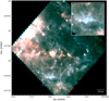 |
Fig. 1 Three colour image of the PLCKECC G074.11+00.11. The colours correspond to SPIRE and PACS observations at wavelengths 160 μm (in red), 250 μm (in green), and 350 μm (in blue). The white rectangle shows the extent of the CO observations. |
3 Results
3.1 Dust continuum observations
The SPIRE observations at 250, 350, and 500 μm were used to derive the dust optical depth at 250 μm and to estimate the H2 column density. We convolved the surface brightness maps to a common resolution of 40′′ and applied average colour correction factors described by Sadavoy et al. (2013). The final colour temperatures were computed by fitting the spectral energy distributions (SEDs) with modified black-body curves with a constant opacity spectral index of β = 1.8. Although the exact value of the spectral index is know to vary from cloud to cloud, β = 1.8 can be taken as an average value in molecular clouds (Planck Collaboration XXII 2011; Planck Collaboration XXIII 2011; Planck Collaboration XXV 2011; Juvela et al. 2015). Furthermore, using a constant spectral index has been shown to reduce biases in the derived parameters (Men’shchikov 2016). The 250 μm optical depth is given by
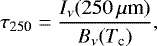 (1)
(1)
where Iν(250 μm) is the fitted 250 μm intensity and Tc is the colour temperature. The data were weighted according to 7% error estimates for SPIRE surface brightness measurements. The hydrogen column density N(H2) was then solved from
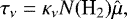 (2)
(2)
where κν is the dust opacity and  is the total gas mass per H2 molecule, 2.8 amu. We assume a dust opacity of κν = 0.1(ν∕1000 GHz)β cm 2 g −1 (Beckwith et al. 1990). The resulting H2 column density and colour temperature maps are shown in Fig. 4. The central region of the clump reaches a column density of ~4.0 × 1022 cm −2 and a temperature of ~12 K. The filament-like structures around the clump are almost as dense and cold as the central region of the clump, with column densities in the range [1–2] × 1022 cm −2 and temperatures in the range [14– 16] K. The assumed error estimates cause an uncertainty of ~1% in the temperature and an uncertainty of ~8% in the column density. The filamentary structures are faint but appear to be continuous in the Herschel images. The structures are also visible in the 12 μm map obtained by the Wide-field Infrared Explorer (WISE, see Fig. A.5), confirming that the structures are continuous and extend several parsecs away from the central clump.
The SCUBA-2 observations at 850 μm trace the densest region of the clump and clearly show smaller dense substructures (labelled S2 to S7 in Fig. 2) above the central clump. The densest ridge of the central clump, S1, has an elliptical shape with the major axis along the northeast-southwest direction. The 850 μm emission shows three separate intensity peaks in the central region of the clump, but only one of the peaks, C1, has a corresponding point sources in the WISE maps from 3.4 to 12 μm. The 450 μm map suffers from poor S/N, only the brightestpeak of the 850 μm map can be identified, thus, we only use the 850 μm map in our analysis.
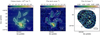 |
Fig. 2 Overview of the dust continuum observations. Left panel: H2 column density map derived form the Herschel observations with the SCUBA-2 observationsat 850 μm shown as contours. Labels C1–C3 indicate three compact sources revealed by SCUBA-2. Middle panel: SCUBA-2 observationsat 850 μm. The circles and ellipses, S1–S7, show the largest substructures in the field and the red crosses show the two continuum sources identified from the SMA observations. Right panel: continuum map derived from the SMA observations; the contours show the SCUBA-2 observations at 850 μm. The area in the right panel corresponds roughly with S1. |
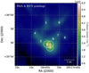 |
Fig. 3 Nine pointings observed with one of the KVN antennas, numbers from 1 to 9, and the SMA pointings shown with circles where the diameter corresponds to the FWHM of the antennas. |
3.2 Spectral lines
Shown in Fig. A.1 are the N2H+ spectra from the KVN pointings shown in Fig. 3. We used the continuum and line analysis single-dish software (CLASS) of the Grenoble image and line data analysis software (GILDAS)4 to make a hyperfine fit to the spectra to estimate the central velocity and the FWHM of the line. For positions 1 to 3 the central velocities increase from − 2.10 ± 0.03 km s−1, to − 0.84 ± 0.03 km s−1, and to 0.25 ± 0.09 km s−1, respectively. The corresponding FWHM values are 2.42 ± 0.1, 2.29 ± 0.1, and 1.5 ± 0.3 km s−1. The spectra from positions 4–9 show variation in the central velocity, with velocities in the range [−2.4, 2.3] km s−1 and FWHM values in the range [0.7, 3.1] km s−1. However, the S/N of the spectra from pointings 4–9 is low, and the fit fails to converge for pointing 8, thus, the resulting hyperfine fits are not accurate. The gradual shift in velocity is also seen in the H2CO line (Fig. A.2) from approximately −2 to approximately 1 km s−1. This could indicate a streaming motion of material flowing along the filaments towards the central clump, or away from the clump (Oya et al. 2014).
We detected H2O maser emission at 22 GHz towards pointings 1 and 9 with the KVN antenna. The H2O maser spectrum of pointing 1 (Fig. 5) has four velocity components lying within 7 km s−1 from the average velocity of the dense gas, while the spectrum from pointing 9 has only two, possibly three, components at −3 km s−1 and at −7 km s−1. We estimate the isotropic luminosity of the maser towards pointing 1, using Eq. (1) of Kim et al. (2018):
 (3)
(3)
where S22 is the integrated flux density of the H2O line at 22 GHz and D is the distance to the source, for which we assumed 2.3 kpc. The distance estimate is discussed in Appendix B. The integrated flux density towards pointing 1 is ~ 20 Jy km s−1 and the estimated isotropic luminosity of the maser emission is L22 ~ 2.43 × 10⁻⁶ L⊙. Towards pointing 1, we have also a clear detection of HCO+ (Fig. A.3). The line profile of HCO+ shows a weak broadening towards higher velocities. To quantify the asymmetry we computed an asymmetry parameter δv defined by Mardones et al. (1997),
 (4)
(4)
where vthick and vthin are the central velocities of the optically thick and thin lines, for which we use the HCO+ and N2H+, respectively, and Δvthin is the FWHM of the optically thin line. For the N2H+ line we use the results of the hyperfine fit from position 1 and for the HCO+ line we estimate a central velocity of −2.95 km s−1, resulting in an asymmetry value of δv = −0.35. For asymmetric lines, Mardones et al. (1997) used the criterion  , thus in our case the HCO+ line has a clear blue asymmetry. The detection of a H2O maser and the asymmetry of the HCO+ line (Fuller et al. 2005) are suggestive of star formation activity in the clump.
Shown in Fig. 6 are 13CO J =1–0 spectra extracted from the PMO observations towards the KVN pointings. The spectral profiles from all nine points are very broad, showing emission in the range [−5, 5] km s−1. Several line profiles show clear asymmetry and cannot be fitted with a simple Gaussian profile. Furthermore, the spectra from the northern side of the region, P5-P8, show a separate velocity component at ~ 7 km s−1. Spectra from SMA 12CO observations(Fig. 7) have been extracted from the locations shown in Fig. 8, which show similar broad emission to the PMO observations. The main emission in the SMA observations is in the range [−5, 0] km s−1 and the spectral profiles show clear inverse P-Cygni profiles for cores C1 and C2, an indication of infalling material. Furthermore, the SMA spectra C3A and C3B have broad wings extending up to approximately −15 km s−1, which can indicate outflows from the compact source C3. The spectra from C1 and C2 also have wings in the line profile, but they are not as broad as for C3. The spectrum C3A also has a separate weak velocity component at 7 km s−1.
Summary of the spectral lines that were observed with the single dish antennas.
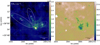 |
Fig. 4 H2 column density map (left panel) and a colour temperature map (right panel) derived from the Herschel observations. The ellipses F1 and F2 show the two filamentary structures connected to the central clump. The dashed ellipse F3 shows the location of the possible third filamentary structure. |
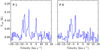 |
Fig. 5 Spectra of the detected H2O maser emission from pointings 1 and 9 (see Fig. 3) using the KVN antenna. |
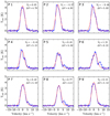 |
Fig. 6 Extracted 13CO J = 1– 0 spectra from the PMO observations towards the KVN pointings shown in Fig. 3. The red line is a Gaussian fit to the line profile and the numbers in the top-right corner are the Gaussian parameters of the fit in km s −1. |
3.3 Kinematics
Integrated intensity and velocity maps from Gaussian fits to the PMO 12CO and 13CO J =1–0 observationsshow two or three filamentary structures and the central clump at a clearly lower average velocity (Figs. 9a–f). The integrated intensity maps are computed over the range [ − 6, 10] km s−1 (panels a and d), and show that the central clump appears elongated along a southeast-northwest direction, while two of the filamentary structures point towards the northeast (F1 and F2 in Fig. 4). A possible third filament F3 extends towards the west. However, it is not evident in the 13CO velocity maps; furthermore the line width maps of the 12CO line show extremely broad line widths and a higher velocity at the western side of the region compared to the clump or filaments F1 and F2. Thus filament F3 is likely a completely separate velocity component on the same line of sight.
Shown in Figs. 9g,h are the moment maps of the 13CO J =2–1 observations from the SMT. Compared to the 13CO observationsfrom PMO, the integrated intensity and the velocity maps are similar, showing wider line widths on the eastern side of the clump. However, there appears to be a coherent structure at the southern side of the clump in the velocity and the line width maps,which is not seen in the PMO maps. Furthermore, in the integrated intensity map (integrated over the range [ − 5.5, 4.5] km s−1; panel g) theclump appears to be elongated towards the northwest-southeast, whereas in the dust continuum maps (Fig. 2), the clump is more elongated in the northeast-southwest direction. The FWHM maps from both SMT and PMO (Figs. 9c,f,i) show coherent line widths for the clump and the filaments F1 and F2.
Shown in Fig. 10 are the PMO 13CO J =1–0 line observations integrated over 2 km s−1 wide velocity intervals. The 13CO line shows a large spread in velocity, ranging from −4 to 5 km s−1, with the main emission seen in the range [−2, 0] km s−1 and the central clump is clearly seen in the range [−4, 0] km s−1. Overall the 13CO line is concentrated around the main clump and traces the two or three low density filaments. The 13CO J =2–1 channel maps (Fig. A.4) are similar to Fig. 10, showing the clump in the range [−4, 0] km s−1, and tracing the filamentary structure F2in the range [0–2] km s−1.
Shown in Fig. 11 are the SMA 12CO and 13CO J =2–1 line observations integrated over 2.4 km s−1 wide velocity intervals. The 13CO channel maps reveal three compact sources in the range [−5, 1.5] km s−1, all associated with an emission peak in the SCUBA-2 map. The contour maps do not show any steep velocity gradients and they do not show any evidence of filamentary structures in the largest velocity bins as seen in the PMO observations, indicating a more isotropic accretion on the point sources from the surrounding medium. The SMA 12CO line shows more of the diffuse emission but, similar to the 13CO observations, shows no trace of the filamentary structures continuing within the clump.
To study possible velocity gradients in the field we draw position–velocity (PV) maps along the lines shown in Fig. 12. The cuts were chosen to trace structures that appear continuous and filamentary in the N(H2) map or in the total integrated intensity map of the 13CO line. For the PV maps in Fig. 13, we use the PMO 13CO J =1–0 observations. In all three cuts a filamentary structure can be seen in the range [0− 2] km s−1 and the emission is seen as a continuous structure. The central clump is at a lower velocity ~ [−2, −1] km s−1 than the filamentary structures. Furthermore, in the vicinity of the clump, the 13CO emission is clearly curved towards the clump, a possible indication of infall or of material flowing out from the clump (Lee et al. 2000). The cut from point 3 to point 4 clearly shows a separate velocity component at higher velocity, in the range [6−8] km s−1, as previously shown.
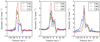 |
Fig. 7 Spectra of the 12CO J = 2– 1 line obtained with the SMA towards positions indicated in Fig. 8. |
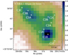 |
Fig. 8 Locations within the central clump where we have extracted the SMA 12CO J = 2– 1 spectra (white crosses). The colour map shows the SCUBA-2 intensity at 850 μm. |
3.4 Mass estimates
We computethe mass of the clump from both the Herschel observations and the SCUBA-2 observations. The mass can be derived from the total hydrogen column density following the equation
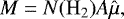 (5)
(5)
where  is the total gas mass per H2 molecule, 2.8 amu, and A is the area of the region. With the assumed distance, the mass of the central clump above a threshold of N(H2) = 2 × 1022 cm−2 is ~ 700 M⊙. To estimate the virial state of the region, we use the N2H+ line and the equation
 (6)
(6)
(MacLaren et al. 1988), where k depends on the assumed density distribution, G is the gravitational constant, and R is the radius of the region. We assumed a density distribution with ρ(r) ∝r−1.5, and thus, k ≈ 1.33 (Chandler & Richer 2000; Whitworth & Ward-Thompson 2001). The total velocity dispersion, σ, including thermal and non-thermal components, was calculated from the equation (Shinnaga et al. 2004)
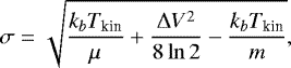 (7)
(7)
where ΔV is the FWHM of the line used, m is the mass of the observed molecule, and μ is the mean molecular mass, 2.33 amu, assuming 10% helium. We assumed a constant kinetic temperature of Tkin = 15 K, which is an average value over the region derived from the Herschel observations. The total hydrogen column density, the shapes and radii of the regions, and the masses and virial masses of the regions are summarised in Table 2. We use a Monte Carlo method to compute the error estimates and assume normally distributed errors. The virial mass estimates for regions 4–7 are uncertain due to the low S/N of the N2H+ observations.
The mass of the region can also be derived from the SCUBA-2 observations. Following Hildebrand (1983), the mass of the region is proportional to the integrated flux density
 (8)
(8)
where Sd is the flux density, D is the distance to the cloud, B850(Td) is the Planck function at 850 μm with dust temperature Td, and κ850 is the opacity at 850 μm. We use a constant dust temperatureof Td = 15 K and for dust opacity we assume κν = 0.1(ν∕1000 GHz)β cm 2 g −1 (Beckwith et al. 1990).
Integrating the surface brightness of the 850 μm band over the central clump and assuming a distance of 2.3 kpc gives an estimated mass of M850 = 230 M⊙. The discrepancy between the SCUBA-2 estimate and the estimate of ~700 M⊙ derived from the Herschel observations, is caused by the spatial filtering of the SCUBA-2 maps (Chapin et al. 2013). The level of filtering depends on the source properties, with an extended source suffering from heavier filtering (Ward-Thompson et al. 2016; Liu et al. 2018). The SCUBA-2 850 μm map is also used to compute the masses of the three compact sources (C1, C2, and C3 in Fig. 2). Assuming a simple circular geometry for the sources, the resulting masses are 36, 13, and 49 M⊙, for C1, C2, and C3, respectively. The estimated virial masses of the compact sources are 2.0, 1.6, and 2.95 M⊙, where we have used the SMA 13CO J = 2–1 observations and Eq. (7) to compute the velocity dispersion.
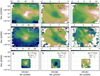 |
Fig. 9 Integrated intensity maps, the average velocity, and line width maps derived from Gaussian fits. The maps are derived formthe PMO 12CO and 13CO J = 1– 0 and SMT 13CO J = 2– 1 observations, panels a–f and g–i, respectively. |
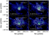 |
Fig. 10 Channel maps of the 13CO J = 1– 0 line emission as observed with the PMO (white contours), superposed on the N(H2) map. The line intensities are integrated over 2.0 km s−1 wide velocity intervals. The velocity centroids are indicated in the top right of each panel and the numbers in the bottom left show the maximum integrated intensity of the bin. |
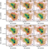 |
Fig. 11 Submillimetre Array 12CO (upper row) and 13CO (lower row) J = 2–1 line observations (red contours) integrated over 2.4 km s−1 wide velocity intervals and plotted over the SCUBA-2 observations at 850 μm. The numbers in the lower left corner show the centre of the velocity bin and the numbers at the top show the maximum intensity of the bin. The beam size is indicated by the blue ellipse in the lower right corner. The white crosses show the location of the three compact sources. |
3.5 Young stellar object
The central clump is associated with the infrared astronomical satellite (IRAS) source 20160+3546, which is well aligned with the compact source C1. We estimate the bolometric luminosity of the IRAS source by making a modified black-body fit to the dust continuum observations from both Herschel and SCUBA-2, covering wavelengths from 70 to 850 μm. The intensity at each wavelength is computed from a circular aperture with a radius corresponding to two times the FWHM of the observations and assuming a constant opacity spectral index of β = 1.8. The resulting best-fit temperature is Tf ~ 25 K and the luminosity of the IRAS source is ~15 L⊙.
4 Discussion
4.1 Cloud structure
Based on the Herschel and WISE images, the clump is associated with parsec-scale, curved filamentary structures or arms that appear to be crossing at the location of the clump. The clump in turn may have formed as a result of a collision of those large-scale structures, as discussed in Sect. 4.2. The clump has further fragmented into three cores. Assuming a distance of 2.3 kpc (see Appendix B), the total mass of the clump is ~700 M⊙, which is ~ 30% of the total mass of the cloud, while the curved filamentary structures have about 1/3 of the mass of the clump. The SCUBA-2 observationshave revealed three compact sources within the clump with estimated masses in the range [10, 50] M⊙.
4.2 Filamentary structures
The low resolution 12CO and 13CO J =1–0 observations show that the central clump is located at a crossing of two, possibly three, large-scale filaments. The line emission shows a large spread in velocities over a range of ~10 km s−1 over the whole region, while the main emission around the clump is seen in the range [−4, 0] km s−1. The two main filamentary structures are seen in the velocity range [0, 2] km s−1, and a possible third fainter filament or separate velocity component in the range [3, 4] km s−1. The PV diagrams of the 13CO J = 1–0 line show that the filaments are continuous structures and appear curved towards the clump in the PV diagrams. The curvature in the PV maps can be interpreted as material flowing towards the central clump. Furthermore, the N2H+ spectra towards pointings 1 to 3 show a clear shift in velocity, which can be interpreted as a streaming motion. Thus, as the clump is found at a crossing of filaments, and since the filaments are connected, at least kinematically to the clump (see Fig. 13), the clump may have formed through compression by colliding filaments and is still accreting material along the filaments. The curved structures seen in the Herschel observations could then have formed by converging flows or by fragmentation within the collapsing cloud. However, at smaller scales, the SMA observations do not show the filamentary structures connecting to the compact sources seen within the clump, but rather the SMA observations seem to trace a shell-like structure around the central clump, indicating a more isotropical mass accretion on the compact sources. This combination of large-scale filamentary structures and smaller scale isotropic accretion conforms with the hybrid model discussed by Myers (2011).
A rough estimate can be derived for mass accretion along the substructure S2 onto the central clump, by assuming a simple relation of a core accreting material along a cylindrical structure (following roughly López-Sepulcre et al. 2010)
 (9)
(9)
where Mf is the mass of the filamentary structure, Lf is the length of thefilament, and  is the velocity. For the length and mass of the filament we use values of Mf = 340 M⊙ and Lf = 1.5 pc, corresponding to the substructure S2. As for the velocity we use a value
  km s−1, the difference between the velocity of the N2H+ hyperfine components from pointings 1 and 3. With the above values, we estimate an accretion rate of 4.3 × 10⁻⁴ M⊙ yr−1. The derived accretion rate is similar to the values reported by Lu et al. (2018) from their observations of high mass star-forming regions and similar to the value estimated by Myers (2009). Thus, the estimated mass accretion rate is sufficient for intermediate-mass- and even high-mass-star formation.
4.3 Compact sources
The central clump is associated with the far-infrared source IRAS 20160+3546. WISE observations show that the central region, which was unresolved by IRAS, contains several near-infrared (NIR) and mid-infrared (MIR) sources within the central region of the clump. The WISE observations at 3.4 and 12 μm are shown in Fig. A.5. Furthermore, the SCUBA-2 maps at 850 μm show three compact sources within the central clump, but the SMA observations show two continuum sources and three point sources in 13CO, within the clump. The distances between the three sources are between 0.3 and 0.5 pc, which is close to the Jeans’ length (Chandrasekhar & Fermi 1953)
 (10)
(10)
where cs is the sound speed, G is the gravitational constant, and ρ is the density. Assuming a temperature of 15 K, the sound speed is cs = 0.21 km s−1, and inserting an average value of ρ over the central clump ρ = 1.65 × 10⁻²⁰ g cm−3, one gets a Jeans length of λJ = 0.35 pc.
One of the SMA continuum sources, C1, is clearly seen in the 13CO and has a clear counterpart in all four WISE channels. The second continuum source, C2, is associated with broader 13CO emission and has no clear counterparts in the MIR, although the source is close to an extended source seen in the WISE 3.4 and 4.6 μm maps. On the other hand, the third source, C3, is not seen in the SMA continuum but is seen in SMA 13CO observations. The source C3 is not seen in MIR,but at 3.6 and 4.6 μm there is a point source close to the location of C3. However, this point source is likely a foreground star as it can be identified in the r, i, and Hα band photometry from the IPHAS survey (The INT Photometric Hα Survey of the Northern Galactic Plane, Drew et al. 2005). Furthermore, all three sources have clear counterparts in the SCUBA-2 map at 850 μm. Thus, it seems that the clump is forming a cluster of at least three stars, all of which are likely in different stages of evolution, judging from the differences in the wavelength coverage. The differences in detections are summarised in Table 3.
Summary of detections towards the compact sources C1–C3.
4.4 Star formation
The H2O maser spectrum detected with the KVN antenna has four velocity components lying within 7 km s−1 of the average velocity of the dense gas. The central velocity component of the H2O maser at approximately −3 km s−1 corresponds to the average velocity of the CO lines. Similarly, the H2O velocity component at ~4 km s−1 corresponds to a velocity component seen in the SMA CO spectra. However, the H2O component at − 7 km s−1 is only seenin the SMA CO observations towards the KVN pointing 2. Furthermore, the HCO+ spectrum has an asymmetric line profile that could indicate an outflow, although the asymmetry is weak. On the other hand, the SMA 12CO J =2–1 line shows clear inverse P-Cygni profiles towards two of the three compact sources (see Figs. 8 and 7) and the C1 and C3 have broad wings in the line profiles. All these features are signatures of star formation.
Several studies have reported a correlation between the bolometric luminosity of a source and the isotropic luminosity of a H2O maser (Bae et al. 2011; Brand et al. 2003; Furuya et al. 2003). We estimated the isotropic luminosity of the H2O maser towards pointing 1 to be L22 ~ 2.43 × 10⁻⁶ L⊙ and derive a bolometric luminosity of 15 L⊙ for the IRAS source. Assuming that the H2O maser towards pointing 1 and the IRAS source are connected, we compare the above values with Fig. 9 from Bae et al. (2011), which place our source at the lower end of intermediate mass young stellar objects, but with a noticeably higher maser luminosity. However, connecting the H2O maser with one of the compact sources is not straightforward since the beam size of the KVN antenna at 22 GHz is ~ 120′′, which for pointings 1 and 9 covers the entire central clump. Only one of the compact objects, C3, shows emission at velocities lower than −6 km s−1 in the SMA 12CO spectra. On the other hand, since the component at ~4 km s−1 is only seen towards pointing 1, it is possible that the clump has two maser sources.
The maser emission, requiring densities of ~109 cm−3 and temperatures around 500 K (Elitzur et al. 1989), is probably caused by shocks in places where protostellar jets hit the surrounding cloud. However, the SMA CO channel maps and spectra show only weak signs of outflows within the clump. On the other hand, because the H2O profile from pointing 1 has three or four symmetric components, the maser emission could be produced by an accretion disc (Cesaroni 1990). A more detailed study would be required to draw conclusions on the nature of the maser emission, but the low temperature and feeble signs of other stellar feedback inside the central clump indicate that the processes leading to star formation have just recently begun.
5 Conclusions
We have studied a star-forming region, G074.11+00.11. The region comprises a large central clump and several filamentary structures and smaller arms that appear to be interconnected. The central clump is nearly circular, but the densest ridge is clearly elongated from northeast to southwest and is aligned with a low density filamentary structure. Furthermore, our molecular line observationsshow that the filamentary structures are kinematically connected with the central clump. Thus, the clump seems to have formed through a collision of structures at a larger scale. The main results of our study are:
-
Based onthe Herschel and SCUBA-2 observations, the mass of the central clump is ~700 M⊙, assuming a distance of 2.3 kpc. The filamentary structures surrounding the central clump have masses in the range [50, 340] M⊙ and the total mass of the region is well in excess of 2500 M⊙.
-
The central clump harbours an IRAS point source, which in our SCUBA-2 and SMA observations is resolved into three compact objects. Two of these are associated with SMA continuum sources and all three can be identified from SMA CO observations and from the SCUBA-2 observations. However, the three sources behave very differently at WISE wavelengths, a possible indication of different evolutionary stages. We derive a bolometric luminosity of ~15 L⊙ for the IRAS source and an estimated temperature of ~25 K.
-
The 12CO and 13CO lines are broad, with velocities ranging from − 10 to 5 km s−1, while the main emission peak is at − 4 km s−1. Based on the low-resolution PMO and SMT observations, the CO lines do not show separate velocity components, but rather a smooth velocity gradient over the field. The velocity gradient is also visible in the position–velocity diagrams drawn through the central clump.
-
The molecular line spectra along the surrounding filamentary structure S1 show a shift in velocity towards the central clump, indicating an ongoing material flow towards the central region of the clump. However, the SMA observations do not show filamentary structures within the clump, thus any accretion on the compact sources within the clump is likely to proceed isotropically rather than along filaments or through filament fragmentation. The present observations therefore conform to the “hybrid” cluster formation models suggested by Myers (2011), which are isotropic on small scales but filamentary on large scales.
-
We have detected a weak water maser towards two pointings within the central clump, with an estimated isotropic luminosity of L22 = 2.4 × 10⁻⁶ L⊙. The water maser has four velocity components in the range [−10, 5] km s−1, with the central velocity component at − 4 km s−1, which is well aligned with the main CO velocity component. The water maser is likely connected to a weak outflow or generated by an accretion disc. However, because of the large beam size, the exact location of the maser cannot be distinguished.
-
The molecular line spectra extracted from the compact sources show inverse P-Cygni profiles characteristic of infall, and asymmetries indicating accretion or low-velocity outflow. Together with water maser emission, these features signify ongoing star formation. However, the present data show no evidence for high-velocity outflows. We therefore suggest that the region represents a very early stage where feedback from newly born stars has not yet taken effect.
In order to properly study the dynamics, and possible accretion along the filaments, a more detailed large scale molecular line study would be beneficial. For example mapping the entire SCUBA-2 region with high density tracers, such as N2H+, could be used to study and model the region in much higher detail.
Acknowledgements
M.S., J.H., and M.J. acknowledge the support of the Academy of Finland Grant No. 285 769. This work has made use of data from the European Space Agency (ESA) mission Gaia (https://www.cosmos.esa.int/gaia), processed by the Gaia Data Processing and Analysis Consortium (DPAC, https://www.cosmos.esa.int/web/gaia/dpac/consortium). Funding for the DPAC has been provided by national institutions, in particular the institutions participating in the Gaia Multilateral Agreement. The data presented in this paper are based on the ESO-ARO programme ID 196.C-0999(A). K.W. acknowledges support by the National Key Research and Development Program of China (2017YFA0402702), the National Science Foundation of China (11721303), and the starting grant at the Kavli Institute for Astronomy and Astrophysics, Peking University (7101502016).
Appendix A: Additional figures
Figures A.1 and A.2 show the N2H+ and H2CO spectra extracted from the nine pointings shown in Fig. 3 using the KVN antenna. Only the spectra from pointings 1 to 4 is used in our analysis as the S/N of pointings 5 to 9 is low. Shown in Fig. A.3 is the single HCO+ spectrum extracted from pointing 1.
Shown in Fig. A.4 are the PMO 13CO J =2–1 line observations, integrated over 1.0 km s−1 wide velocity intervals. The underlying colour map is the H2 column density map, derived from the Herschel/SPIRE observations.
Shown in Fig. A.5 are the 3.4 and 12 μm observationsfrom the WISE satellite. The central clump is associated with several NIR and MIR point sources and is seen in absorption at 12 μm. The SCUBA-2 observations trace extremely well the regions seen in absorption.
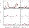 |
Fig. A.1 Spectra of the N2H+ line towards the nine pointings shown in Fig. 3. The red curves show fits to the hyperfine structure of the line components. For pointing 8, the fit fails to converge. |
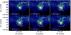 |
Fig. A.4 Channel maps of the 13CO J = 2– 1 line emissionsuperposed on the N(H2) map. The line observations, white contours, are from the PMO and are integrated over 1.0 km s−1 wide velocity intervals. The velocity centroids are indicated in the top right and the maximum integrated intensity in the channel is indicated in the bottom left. |
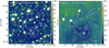 |
Fig. A.5 Images of G074.11+00.11 obtained with the WISE satellite at 3.4 μm (left panel) and 12 μm (right panel). The white contours show the SCUBA-2 map at 850 μm. The WISE observations are in the native digital numbers (DN). |
Appendix B: Distance estimation
To estimate the mass of the region, a reliable distance estimate is needed. The distance reported in the Planck catalogue of galactic cold clumps (PGCC) catalogue is 3.45 kpc (Planck Collaboration XXVIII 2016). This is derived from NIR extinction. On the other hand, assuming a VLSR = −2 km s−1 for the clump, a Bayesian distance estimate (Reid et al. 2016) with no prior information on whether the source is located near or far, Pfar = 0.5, gives the highest probability (P = 0.9) for a distance of4.3 ± 0.7 kpc. The second and third highest probabilities given by the Bayesian method are 2.4 and 1.3 kpc, both of which have a similar probability (P = 0.05 and P = 0.03, respectively). However, estimating distances from kinematics can be unreliable in the Galactic plane, thus, we derive an independent estimate for the distance using a three-dimensional extinction method (Marshall et al. 2006). The best fit from the method gives two components in the line of sight, one at 0.96 ± 0.07 kpc and one at 2.3 ± 0.1 kpc. The estimated visual extinction values given by the method for these components are Av = 1.7 magnitudes and Av ~ 10 magnitudes,respectively.
Since the above methods give three possible distances, although the probability from the Bayesian estimate for the distance of ~ 2 kpc is low, we derive a third independent estimate from the Gaia observations (Gaia Collaboration 2016). The Gaia data release 2 (DR2, Gaia Collaboration 2018) gives the positions, parallaxes, and magnitudes for more than 1.6 billion sources, and provides an excellent tool for distance estimation.
Shown in Fig. B.1 are the locations of ~1000 stars that are used in our distance estimation. The stars were selected from the DR2 catalogue based on two criteria: the value of the line-of-sight extinction in G band is not negative AG > 0, and the parallax-over-error is larger than five  . The parallaxes were then converted to distances by
  , where
  is given in seconds of arc. However, as discussed by Bailer-Jones (2015) and Luri et al. (2018), a priori assumptionsor Bayesian methods should be used when deriving distance estimates from the parallax measurements to get reliable distance estimates, but this exercise is beyond the scope of this paper. Furthermore, the AG values reported in the DR2 catalogue are likely to be incorrect on the star-by-star level, but they should be usable for larger scale studies (Andrae et al. 2018).
The resulting distances as a function of AG are shown in Fig. B.2 for two positions that we call “Cloud” and “Reference” and are indicated in Fig. B.1. The Cloud position covers our target G074.11+00.11. For the Cloud position stars, the median value of AG over a 250 pc wide bin (the black-blue line) is relatively constant until a distance of ~1 kpc, after which the extinction rapidly increases by a factor of approximately four to a median value of 2.3 mag at ~2 kpc. For theReference position stars (black-orange line), the increase of extinction is not as steep, reaching a median value of 1.5 mag at 2 kpc.
Thus, assuming that the increase in the AG is caused only by increasing column density in the line of sight, the lower limit for the distance to the region G074.11+00.11 is ~ 1.25–1.75 kpc. However, taking into account that both the Cloud and Reference positions show an almost constant median value of AG at a distance of ~2 kpc and that the best fit from the extinction method is at ~2 kpc, we assume a distance of 2.3 kpc for the cloud.
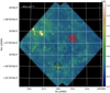 |
Fig. B.1 Locations of the stars from the Gaia data release 2 catalogue used in our distance estimation. The stars in our “Cloud” position are indicated with black markers, and those in the “Reference” position are indicated with red. |
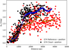 |
Fig. B.2 Line-of-sight extinction in the Gaia G-band as a function of distance. The black and red points correspond to the markers in Fig. B.1. The black-blue and black-orange lines show the median value of AG, computed over a 250 pc wide bins. The width of the blue and orange area corresponds to the error of the mean value of the data points within each bin. |
References
- Alonso-Albi, T., Fuente, A., Bachiller, R., et al. 2009, A&A, 497, 117 [NASA ADS] [CrossRef] [EDP Sciences] [Google Scholar]
- Andrae, R., Fouesneau, M., Creevey, O., et al. 2018, A&A, 616, A8 [NASA ADS] [CrossRef] [EDP Sciences] [Google Scholar]
- André, P., Di Francesco, J., Ward-Thompson, D., et al. 2014, Protostars and Planets VI (Tucson, AZ: University of Arizona Press), 27 [Google Scholar]
- Bae, J.-H., Kim, K.-T., Youn, S.-Y., et al. 2011, ApJS, 196, 21 [NASA ADS] [CrossRef] [Google Scholar]
- Bailer-Jones, C. A. L. 2015, PASP, 127, 994 [NASA ADS] [CrossRef] [Google Scholar]
- Beckwith, S. V. W., Sargent, A. I., Chini, R. S., & Guesten, R. 1990, AJ, 99, 924 [NASA ADS] [CrossRef] [Google Scholar]
- Brand, J., Cesaroni, R., Comoretto, G., et al. 2003, A&A, 407, 573 [NASA ADS] [CrossRef] [EDP Sciences] [Google Scholar]
- Busquet, G., Zhang, Q., Palau, A., et al. 2013, ApJ, 764, L26 [NASA ADS] [CrossRef] [Google Scholar]
- Cesaroni, R. 1990, A&A, 233, 513 [NASA ADS] [Google Scholar]
- Chandler, C. J., & Richer, J. S. 2000, ApJ, 530, 851 [NASA ADS] [CrossRef] [Google Scholar]
- Chandrasekhar, S., & Fermi, E. 1953, ApJ, 118, 116 [NASA ADS] [CrossRef] [MathSciNet] [Google Scholar]
- Chapin, E. L., Berry, D. S., Gibb, A. G., et al. 2013, MNRAS, 430, 2545 [NASA ADS] [CrossRef] [Google Scholar]
- Drew, J. E., Greimel, R., Irwin, M. J., et al. 2005, MNRAS, 362, 753 [NASA ADS] [CrossRef] [Google Scholar]
- Eden, D. J., Liu, T., Kim, K.-T., et al. 2019, MNRAS, 485, 2895 [NASA ADS] [CrossRef] [Google Scholar]
- Elitzur, M., Hollenbach, D. J., & McKee, C. F. 1989, ApJ, 346, 983 [NASA ADS] [CrossRef] [Google Scholar]
- Fuller, G. A., Williams, S. J., & Sridharan, T. K. 2005, A&A, 442, 949 [NASA ADS] [CrossRef] [EDP Sciences] [Google Scholar]
- Furuya, R. S., Kitamura, Y., Wootten, A., Claussen, M. J., & Kawabe, R. 2003, ApJS, 144, 71 [NASA ADS] [CrossRef] [Google Scholar]
- Gaia Collaboration (Prusti, T., et al.) 2016, A&A, 595, A1 [NASA ADS] [CrossRef] [EDP Sciences] [Google Scholar]
- Gaia Collaboration (Brown, A. G. A., et al.) 2018, A&A, 616, A1 [NASA ADS] [CrossRef] [EDP Sciences] [Google Scholar]
- Galván-Madrid, R., Zhang, Q., Keto, E., et al. 2010, ApJ, 725, 17 [NASA ADS] [CrossRef] [Google Scholar]
- Giannetti, A., Brand, J., Sánchez-Monge, Á., et al. 2013, A&A, 556, A16 [NASA ADS] [CrossRef] [EDP Sciences] [Google Scholar]
- Griffin, M. J., Abergel, A., Abreu, A., et al. 2010, A&A, 518, L3 [Google Scholar]
- Hildebrand, R. H. 1983, QJRAS, 24, 267 [NASA ADS] [Google Scholar]
- Ho, P. T. P., Moran, J. M., & Lo, K. Y. 2004, ApJ, 616, L1 [NASA ADS] [CrossRef] [Google Scholar]
- Holland, W. S., Bintley, D., Chapin, E. L., et al. 2013, MNRAS, 430, 2513 [NASA ADS] [CrossRef] [Google Scholar]
- Juvela, M., Ristorcelli, I., Marshall, D. J., et al. 2015, A&A, 584, A93 [NASA ADS] [CrossRef] [EDP Sciences] [Google Scholar]
- Karr, J. L., & Martin, P. G. 2003, ApJ, 595, 900 [NASA ADS] [CrossRef] [Google Scholar]
- Kim, C.-H., Kim, K.-T., & Park, Y.-S. 2018, ApJS, 236, 31 [NASA ADS] [CrossRef] [Google Scholar]
- Lee, H.-T., & Chen, W. P. 2007, ApJ, 657, 884 [NASA ADS] [CrossRef] [Google Scholar]
- Lee, C.-F., Mundy, L. G., Reipurth, B., Ostriker, E. C., & Stone, J. M. 2000, ApJ, 542, 925 [NASA ADS] [CrossRef] [Google Scholar]
- Liu, H. B., Quintana-Lacaci, G., Wang, K., et al. 2012a, ApJ, 745, 61 [NASA ADS] [CrossRef] [Google Scholar]
- Liu, H. B., Jiménez-Serra, I., Ho, P. T. P., et al. 2012b, ApJ, 756, 10 [NASA ADS] [CrossRef] [Google Scholar]
- Liu, T., Wu, Y., & Zhang, H. 2012c, ApJS, 202, 4 [NASA ADS] [CrossRef] [Google Scholar]
- Liu, T., Wu, Y., & Zhang, H. 2013, ApJ, 775, L2 [NASA ADS] [CrossRef] [Google Scholar]
- Liu, H. B., Galván-Madrid, R., Jiménez-Serra, I., et al. 2015, ApJ, 804, 37 [NASA ADS] [CrossRef] [Google Scholar]
- Liu, T., Zhang, Q., Kim, K.-T., et al. 2016, ApJ, 824, 31 [NASA ADS] [CrossRef] [Google Scholar]
- Liu, T., Kim, K.-T., Juvela, M., et al. 2018, ApJS, 234, 28 [NASA ADS] [CrossRef] [Google Scholar]
- López-Sepulcre, A., Cesaroni, R., & Walmsley, C. M. 2010, A&A, 517, A66 [NASA ADS] [CrossRef] [EDP Sciences] [Google Scholar]
- Lu, X., Zhang, Q., Liu, H. B., et al. 2018, ApJ, 855, 9 [NASA ADS] [CrossRef] [Google Scholar]
- Luri, X., Brown, A. G. A., Sarro, L. M., et al. 2018, A&A, 616, A9 [NASA ADS] [CrossRef] [EDP Sciences] [Google Scholar]
- MacLaren, I., Richardson, K. M., & Wolfendale, A. W. 1988, ApJ, 333, 821 [NASA ADS] [CrossRef] [Google Scholar]
- Mardones, D., Myers, P. C., Tafalla, M., et al. 1997, ApJ, 489, 719 [NASA ADS] [CrossRef] [Google Scholar]
- Marshall, D. J., Robin, A. C., Reylé, C., Schultheis, M., & Picaud, S. 2006, A&A, 453, 635 [NASA ADS] [CrossRef] [EDP Sciences] [Google Scholar]
- Meng, F., Wu, Y., & Liu, T. 2013, ApJS, 209, 37 [NASA ADS] [CrossRef] [Google Scholar]
- Men’shchikov, A. 2016, A&A, 593, A71 [NASA ADS] [CrossRef] [EDP Sciences] [Google Scholar]
- Molinari, S., Swinyard, B., Bally, J., et al. 2010, A&A, 518, L100 [NASA ADS] [CrossRef] [EDP Sciences] [Google Scholar]
- Myers, P. C. 2009, ApJ, 706, 1341 [NASA ADS] [CrossRef] [Google Scholar]
- Myers, P. C. 2011, ApJ, 735, 82 [NASA ADS] [CrossRef] [Google Scholar]
- Oya, Y., Sakai, N., Sakai, T., et al. 2014, ApJ, 795, 152 [NASA ADS] [CrossRef] [Google Scholar]
- Padoan, P., Juvela, M., Goodman, A. A., & Nordlund, Å. 2001, ApJ, 553, 227 [NASA ADS] [CrossRef] [Google Scholar]
- Peretto, N., Fuller, G. A., Duarte-Cabral, A., et al. 2013, A&A, 555, A112 [NASA ADS] [CrossRef] [EDP Sciences] [Google Scholar]
- Planck Collaboration XXII. 2011, A&A, 536, A22 [NASA ADS] [CrossRef] [EDP Sciences] [Google Scholar]
- Planck Collaboration XXIII. 2011, A&A, 536, A23 [NASA ADS] [CrossRef] [EDP Sciences] [Google Scholar]
- Planck Collaboration XXV. 2011, A&A, 536, A25 [NASA ADS] [CrossRef] [EDP Sciences] [Google Scholar]
- Planck Collaboration XXVIII. 2016, A&A, 594, A28 [NASA ADS] [CrossRef] [EDP Sciences] [Google Scholar]
- Poglitsch, A., Waelkens, C., Geis, N., et al. 2010, A&A, 518, L2 [NASA ADS] [CrossRef] [EDP Sciences] [Google Scholar]
- Reid, M. J., Dame, T. M., Menten, K. M., & Brunthaler, A. 2016, ApJ, 823, 77 [NASA ADS] [CrossRef] [Google Scholar]
- Sadavoy, S. I., Di Francesco, J., Johnstone, D., et al. 2013, ApJ, 767, 126 [NASA ADS] [CrossRef] [Google Scholar]
- Shan, W., Yang, J., Shi, S., et al. 2012, IEEE Trans. Terahertz Sci. Technol., 2, 593 [NASA ADS] [CrossRef] [Google Scholar]
- Shinnaga, H., Ohashi, N., Lee, S.-W., & Moriarty-Schieven, G. H. 2004, ApJ, 601, 962 [NASA ADS] [CrossRef] [Google Scholar]
- Tan, J. C., Beltrán, M. T., Caselli, P., et al. 2014, Protostars and Planets VI (Tucson, AZ: University of Arizona Press), 149 [Google Scholar]
- Wang, P., Li, Z.-Y., Abel, T., & Nakamura, F. 2010, ApJ, 709, 27 [NASA ADS] [CrossRef] [Google Scholar]
- Wang, K., Zahorecz, S., Cunningham, M. R., et al. 2018, Res. Notes AAS, 2, 2 [NASA ADS] [CrossRef] [Google Scholar]
- Ward-Thompson, D., Pattle, K., Kirk, J. M., et al. 2016, MNRAS, 463, 1008 [NASA ADS] [CrossRef] [Google Scholar]
- Whitworth, A. P., & Ward-Thompson, D. 2001, ApJ, 547, 317 [NASA ADS] [CrossRef] [Google Scholar]
- Wu, Y., Liu, T., Meng, F., et al. 2012, ApJ, 756, 76 [NASA ADS] [CrossRef] [Google Scholar]
- Yuan, J., Li, J.-Z., Wu, Y., et al. 2018, ApJ, 852, 12 [NASA ADS] [CrossRef] [Google Scholar]
All Tables
All Figures
|
Fig. 1 Three colour image of the PLCKECC G074.11+00.11. The colours correspond to SPIRE and PACS observations at wavelengths 160 μm (in red), 250 μm (in green), and 350 μm (in blue). The white rectangle shows the extent of the CO observations. |
| In the text | |
|
Fig. 2 Overview of the dust continuum observations. Left panel: H2 column density map derived form the Herschel observations with the SCUBA-2 observationsat 850 μm shown as contours. Labels C1–C3 indicate three compact sources revealed by SCUBA-2. Middle panel: SCUBA-2 observationsat 850 μm. The circles and ellipses, S1–S7, show the largest substructures in the field and the red crosses show the two continuum sources identified from the SMA observations. Right panel: continuum map derived from the SMA observations; the contours show the SCUBA-2 observations at 850 μm. The area in the right panel corresponds roughly with S1. |
| In the text | |
|
Fig. 3 Nine pointings observed with one of the KVN antennas, numbers from 1 to 9, and the SMA pointings shown with circles where the diameter corresponds to the FWHM of the antennas. |
| In the text | |
|
Fig. 4 H2 column density map (left panel) and a colour temperature map (right panel) derived from the Herschel observations. The ellipses F1 and F2 show the two filamentary structures connected to the central clump. The dashed ellipse F3 shows the location of the possible third filamentary structure. |
| In the text | |
|
Fig. 5 Spectra of the detected H2O maser emission from pointings 1 and 9 (see Fig. 3) using the KVN antenna. |
| In the text | |
|
Fig. 6 Extracted 13CO J = 1– 0 spectra from the PMO observations towards the KVN pointings shown in Fig. 3. The red line is a Gaussian fit to the line profile and the numbers in the top-right corner are the Gaussian parameters of the fit in km s −1. |
| In the text | |
|
Fig. 7 Spectra of the 12CO J = 2– 1 line obtained with the SMA towards positions indicated in Fig. 8. |
| In the text | |
|
Fig. 8 Locations within the central clump where we have extracted the SMA 12CO J = 2– 1 spectra (white crosses). The colour map shows the SCUBA-2 intensity at 850 μm. |
| In the text | |
|
Fig. 9 Integrated intensity maps, the average velocity, and line width maps derived from Gaussian fits. The maps are derived formthe PMO 12CO and 13CO J = 1– 0 and SMT 13CO J = 2– 1 observations, panels a–f and g–i, respectively. |
| In the text | |
|
Fig. 10 Channel maps of the 13CO J = 1– 0 line emission as observed with the PMO (white contours), superposed on the N(H2) map. The line intensities are integrated over 2.0 km s−1 wide velocity intervals. The velocity centroids are indicated in the top right of each panel and the numbers in the bottom left show the maximum integrated intensity of the bin. |
| In the text | |
|
Fig. 11 Submillimetre Array 12CO (upper row) and 13CO (lower row) J = 2–1 line observations (red contours) integrated over 2.4 km s−1 wide velocity intervals and plotted over the SCUBA-2 observations at 850 μm. The numbers in the lower left corner show the centre of the velocity bin and the numbers at the top show the maximum intensity of the bin. The beam size is indicated by the blue ellipse in the lower right corner. The white crosses show the location of the three compact sources. |
| In the text | |
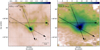 |
Fig. 12 Positions and directions (black arrows) of the position–velocity maps shown in Fig. 13. |
| In the text | |
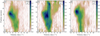 |
Fig. 13 Position–velocity maps of the 13CO J = 1– 0 line drawn along the lines shown in Fig. 12. |
| In the text | |
|
Fig. A.1 Spectra of the N2H+ line towards the nine pointings shown in Fig. 3. The red curves show fits to the hyperfine structure of the line components. For pointing 8, the fit fails to converge. |
| In the text | |
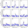 |
Fig. A.2 Spectra of the H2CO line towardsthe nine pointings shown in Fig. 3. |
| In the text | |
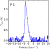 |
Fig. A.3 Spectrum of the HCO+ line towardspointing 1 in Fig. 3. |
| In the text | |
|
Fig. A.4 Channel maps of the 13CO J = 2– 1 line emissionsuperposed on the N(H2) map. The line observations, white contours, are from the PMO and are integrated over 1.0 km s−1 wide velocity intervals. The velocity centroids are indicated in the top right and the maximum integrated intensity in the channel is indicated in the bottom left. |
| In the text | |
|
Fig. A.5 Images of G074.11+00.11 obtained with the WISE satellite at 3.4 μm (left panel) and 12 μm (right panel). The white contours show the SCUBA-2 map at 850 μm. The WISE observations are in the native digital numbers (DN). |
| In the text | |
|
Fig. B.1 Locations of the stars from the Gaia data release 2 catalogue used in our distance estimation. The stars in our “Cloud” position are indicated with black markers, and those in the “Reference” position are indicated with red. |
| In the text | |
|
Fig. B.2 Line-of-sight extinction in the Gaia G-band as a function of distance. The black and red points correspond to the markers in Fig. B.1. The black-blue and black-orange lines show the median value of AG, computed over a 250 pc wide bins. The width of the blue and orange area corresponds to the error of the mean value of the data points within each bin. |
| In the text | |
Current usage metrics show cumulative count of Article Views (full-text article views including HTML views, PDF and ePub downloads, according to the available data) and Abstracts Views on Vision4Press platform.
Data correspond to usage on the plateform after 2015. The current usage metrics is available 48-96 hours after online publication and is updated daily on week days.
Initial download of the metrics may take a while.