| Issue |
A&A
Volume 629, September 2019
|
|
|---|---|---|
| Article Number | A91 | |
| Number of page(s) | 17 | |
| Section | Catalogs and data | |
| DOI | https://doi.org/10.1051/0004-6361/201935916 | |
| Published online | 10 September 2019 | |
Evolved massive stars at low-metallicity
I. A source catalog for the Small Magellanic Cloud⋆
1
IAASARS, National Observatory of Athens, Vas. Pavlou and I. Metaxa, Penteli 15236, Greece
e-mail: This email address is being protected from spambots. You need JavaScript enabled to view it.
2
Department of Astronomy, Beijing Normal University, Beijing 100875, PR China
3
Rhea Group for ESA/ESAC, Camino bajo del Castillo, s/n, Urbanizacion Villafranca del Castillo, Villanueva de la Canada 28692, Madrid, Spain
4
Key Laboratory of Optical Astronomy, National Astronomical Observatories, Chinese Academy of Sciences, Datun Road 20A, Beijing 100101, PR China
5
International Centre for Radio Astronomy Research, Curtin University, Bentley, WA 6102, Australia
6
Department of Astrophysics, Astronomy & Mechanics, Faculty of Physics, University of Athens, Zografos 15783, Athens, Greece
Received:
18
May
2019
Accepted:
11
July
2019
Abstract
We present a clean, magnitude-limited (IRAC1 or WISE1 ≤ 15.0 mag) multiwavelength source catalog for the Small Magellanic Cloud (SMC) with 45 466 targets in total, with the purpose of building an anchor for future studies, especially for the massive star populations at low-metallicity. The catalog contains data in 50 different bands including 21 optical and 29 infrared bands, retrieved from SEIP, VMC, IRSF, AKARI, HERITAGE, Gaia, SkyMapper, NSC, Massey (2002, ApJS, 141, 81), and GALEX, ranging from the ultraviolet to the far-infrared. Additionally, radial velocities and spectral classifications were collected from the literature, and infrared and optical variability statistics were retrieved from WISE, SAGE-Var, VMC, IRSF, Gaia, NSC, and OGLE. The catalog was essentially built upon a 1″ crossmatching and a 3″ deblending between the Spitzer Enhanced Imaging Products (SEIP) source list and Gaia Data Release 2 (DR2) photometric data. Further constraints on the proper motions and parallaxes from Gaia DR2 allowed us to remove the foreground contamination. We estimate that about 99.5% of the targets in our catalog are most likely genuine members of the SMC. Using the evolutionary tracks and synthetic photometry from MESA Isochrones & Stellar Tracks and the theoretical J − KS color cuts, we identified 1405 red supergiant (RSG), 217 yellow supergiant, and 1369 blue supergiant candidates in the SMC in five different color-magnitude diagrams (CMDs), where attention should also be paid to the incompleteness of our sample. We ranked the candidates based on the intersection of different CMDs. A comparison between the models and observational data shows that the lower limit of initial mass for the RSG population may be as low as 7 or even 6 M⊙ and that the RSG is well separated from the asymptotic giant branch (AGB) population even at faint magnitude, making RSGs a unique population connecting the evolved massive and intermediate stars, since stars with initial mass around 6 to 8 M⊙ are thought to go through a second dredge-up to become AGB stars. We encourage the interested reader to further exploit the potential of our catalog.
Key words: infrared: stars / Magellanic Clouds / stars: late-type / stars: massive / stars: mass-loss / stars: variables: general
Full Table 3 and tables for RSG, YSG and BSG candidates are only available at the CDS via anonymous ftp to cdsarc.u-strasbg.fr (130.79.128.5) or via http://cdsarc.u-strasbg.fr/viz-bin/qcat?J/A+A/629/A91
© ESO 2019
1. Introduction
Massive stars are those born with initial masses ≳8 M⊙. They are relatively rare compared to the large number of low-mass stars due to the initial mass function and their short lifetimes. However, as a result of the intensive interior energy transfer and radiative output, massive stars are responsible for some of the most extreme astrophysics in the Universe, including supernovae (SN), black holes, gravitational waves, and long gamma-ray bursts, and are critical for stellar evolution, star formation, and chemical evolution throughout cosmic time (Humphreys & McElroy 1984; Woosley et al. 2002; Massey 2003, 2013; Meynet et al. 2011; Maeder & Meynet 2012). The first generation of stars in the early Universe is expected to be massive and one of the main contributors of dust content in high-redshift galaxies (Massey et al. 2005; Bromm et al. 2009; Levesque 2010). Therefore, understanding the physical properties, evolution, and mass loss of massive stars may help to reveal the formation of the primitive cosmic structures (Gall et al. 2011; Smith 2014; Zhang et al. 2018).
Unfortunately, such stages of the early Universe cannot be directly observed. The alternative way is to study analogous systems to the early Universe in our own cosmic backyard. In recent years, there has been a growing interest in massive stars in metal-poor environments due to the advancement of detectors and telescopes and the need to extrapolate the astrophysics from the local Universe to the early cosmic epochs. As a consequence, metal-poor star-forming dwarf irregular (dIrr) galaxies in the local Universe serve as an ideal laboratory for investigating the evolution and mass loss of massive stars at low-metallicity, since they mimic the behaviors of galaxies in the early Universe (Kunth & Östlin 2000; McConnachie 2012).
To understand the evolution of massive stars in low-metallicity environments, both theoretical and observational constraints are needed. Among the many physical parameters of massive stars, one deterministic parameter is the mass loss, which has a profound impact on the lifetime of a star as well as its luminosity (L), effective temperature (Teff), radiation field, and its fate as a supernova (SN). However, the most important modes of mass loss are the most uncertain (Smith 2014). It has been known that the mass-loss rates (MLRs) adopted in modern stellar evolution codes for standard metallicity-dependent winds of hot main sequence stars are overestimated by a factor of two to three due to the clumped and inhomogeneous stellar winds (Puls et al. 2008). Therefore, other factors, for example, the stellar winds, pulsations, rotation, convection, and eruptions of evolved supergiants, as well as binary mass transfer, may provide important contributions to the removal of the hydrogen envelope. Alternatively, overestimation of the MLR of the hot stars may just simply raise the upper mass limit controlling which stars become Wolf-Rayet stars (WRs) through stellar wind mass-loss alone. Meanwhile, it has also been recognized that the unsteady modes of mass loss, like the episodic mass-loss events, are more important than previously thought (Smith & Owocki 2006; Ofek et al. 2013). Consequently, observation in the infrared wavelengths, especially the relatively long wavelengths that are mainly dominated by dust emission, has a great impact on the understanding of MLR of massive stars.
Among the Local Group galaxies, the Large and Small Magellanic Clouds (LMC and SMC) are particularly intriguing due to their low-metallicity environments (about half and one-fifth of the Milky Way; Russell & Dopita 1992; Rolleston et al. 2002; Keller & Wood 2006; Dobbie et al. 2014; D’Onghia & Fox 2016) and close distances, for which individual stars can be resolved, allowing for a detailed analysis of their massive star populations in a variety of ways (Barba et al. 1995; Massey & Olsen 2003; Evans & Howarth 2008; Bonanos et al. 2009, 2010; Neugent et al. 2010; Yang & Jiang 2011, 2012; Bouret et al. 2013; Kourniotis et al. 2014; Hainich et al. 2015; Castro et al. 2018; Yang et al. 2018; Britavskiy et al. 2019; Patrick et al. 2019).
In this paper, we focus on the evolved, dusty massive star population in the SMC. We construct a clean catalog of massive stars, including their infrared properties (related to the MLR), astrometric solution regarding their membership to the SMC, time-series data revealing stellar variability, and evolutionary models in relation to their evolutionary stages, aiming to build a comprehensive anchor for future studies. The paper is structured as follows: the multiwavelength source catalog and time-series data are presented in Sects. 2 and 3, respectively. The identification of evolved massive star candidates is described in Sect. 4. A summary is given in Sect. 5.
2. Multiwavelength source catalog
Since our goal is to focus on the evolved dusty massive stars in the SMC, we use the Spitzer Enhanced Imaging Products (SEIP) source list as a starting point. This list contains sources detected with a high signal-to-noise ratio (S/N at the 10-sigma level) in at least one channel among 12 near-infrared (NIR) to mid-infrared (MIR) bands of J (1.25 μm), H (1.65 μm), KS (2.17 μm), IRAC1 (3.6 μm), IRAC2 (4.5 μm), IRAC3 (5.8 μm), IRAC4 (8.0 μm), MIPS24 (24 μm), WISE1 (3.4 μm), WISE2 (4.6 μm), WISE3 (12 μm), and WISE4 (22 μm), from the Two Micron All Sky Survey (2MASS; Skrutskie et al. 2006), Spitzer (Werner et al. 2004), and Wide-field Infrared Survey Explorer (WISE; Wright et al. 2010)1. We retrieved the initial IR data from the SEIP source list with 3 ° ≤RA ≤ 25°, −75.5 ° ≤Dec ≤ −70° and IRAC1 or WISE1 ≤ 15.0 mag, covering almost the whole SMC and also a small part of the Magellanic Bridge (MB). The magnitude cut of IRAC1 or WISE1 ≤ 15.0 mag was justified based on a drop-off (∼14.85 mag) in the number counts for 12 748 156 ALLWISE WISE1 single-epoch measurements in the same region as shown in Fig. 1. Considering the lower angular resolution of WISE (∼6″) and 2MASS (∼5″) compared to Spitzer (∼2″), and that WISE sources within 3″ of a SEIP source were reported, a deblending was performed with a search radius of 3″. Targets with neighbors within 3″ were excluded from the initial dataset, which resulted in 131 233 targets.
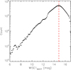 |
Fig. 1. ALLWISE WISE1 single-epoch measurements in the SMC region. A drop-off of 14.85 mag is shown by the red dashed line. |
Besides the IR detection, the reliable membership to the SMC is also a crucial factor for our study, for which the astrometric solution from Gaia Data Release 2 (DR2) is vital (Gaia Collaboration 2016, 2018a). Given the very small offset between the Gaia DR2 and the 2MASS (median value of ∼0.120″ ± 0.157″ for targets with G ≤ 18 mag in the same SMC region), as well as the SEIP source list and the 2MASS (median value of ∼0.089″ ± 0.237″1), we crossmatched the deblended SEIP data and Gaia DR2 with a search radius of 1″ to fix the position, and removed any SEIP targets with multiple counterparts to eliminate the blending. A 3″ crossmatching was then performed and SEIP targets with multiple counterparts were removed again, resulting in 74 237 targets. Since the effective angular resolution of the Gaia DR2 source list has improved to ∼0.4″, with incompleteness in close pairs of stars starting below about 2″ (Gaia Collaboration 2018a; Arenou et al. 2018), we can reasonably assume that the vast majority of the blending is removed at the resolutions of both Spitzer and Gaia.
After crossmatching and deblending between SEIP and Gaia data, the Gaia DR2 astrometric solution was used to eliminate the foreground contamination (Lindegren et al. 2018). The selection of SMC members was restricted to targets with errors < 0.5 mas yr−1 in proper motion (PM) and < 0.5 mas in parallax. The first two panels of Fig. 2 show the errors versus Gaia PMs in RA (left) and Dec (middle), respectively. We fit a Gaussian profile to PM at each dimension as 0.695 (peak)±0.240 (σ) mas yr−1 in RA and −1.206 ± 0.140 mas yr−1 in Dec, and calculated the limits of ±5σ shown as the vertical dashed lines. The last panel (right) of Fig. 2 shows the errors versus Gaia parallaxes. Similarly, a Gaussian profile fitting was adopted for the parallax as −0.009 ± 0.066 mas, while an additional elliptical constraint was also applied with the 5σ limits of PMRA and PMDec taken as the primary and secondary radii, respectively. The same criteria of ±5σ were calculated for the parallax. Briefly, the membership of the SMC is constrained by a Gaussian profile of the parallax with an additional elliptical constraint derived from PMRA and PMDec, which results in 45 466 targets. In addition to the previous astrometric constraints, we also applied a constraint on the radial velocity (RV) for all targets that have Gaia RV measurements, set at approximately RV ≥ 90 km s−1 as shown below.
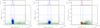 |
Fig. 2. Evaluation of the Gaia astrometric solution. The limits of PM error (0.5 mas yr−1) and parallax error (0.5 mas) are shown as horizontal dashed lines. First two panels: errors vs. Gaia PMs in RA (left) and Dec (middle), respectively. A Gaussian profile is fitted to PM in each dimension and the limits of ±5σ are calculated (vertical dashed lines). The selected targets are shown in blue color. Last panel (right): errors vs. Gaia parallaxes. A Gaussian fitting is adopted again for the parallax, while an additional elliptical constraint has also been applied with the 5σ limits of PMRA and PMDec taken as the primary and secondary radii, respectively. The same criteria of ±5σ were calculated for the parallax (vertical dashed lines). The final selected targets are shown in red color. Green contours show the number density in each diagram. |
Further evaluation of the astrometric excess noise, which measures the disagreement and is expressed as an angle between the observations of a source and the best-fitting standard astrometric model (using five astrometric parameters), shows that about 99.5% of our targets have astrometric_excess_ noise ≤ 0.5 mas, indicating good astrometric solutions for the vast majority of our targets (Lindegren et al. 2018). Moreover, Gaia Collaboration (2018b) determined the PMs and parallaxes for 75 Galactic globular clusters, nine dwarf spheroidal galaxies, one ultra-faint system, and the MCs, where the method was also used by others (see, e.g., Aadland et al. 2018). The basic idea was to first determine the median and robust scatter in PMs and parallaxes by selecting a sample of stars covering a larger field of view (FoV), then further eliminate any sources showing larger scatter in the PMs, and finally construct a filter based on a covariance matrix of the cleaned sample, which allows one to properly select out likely members. Gaia Collaboration (2018b) also provided lists of possible members according to their analysis for all the systems. We crossmatched between our list of 45 466 targets and the Gaia list of ∼1.4 million sources for the SMC (their data covered a larger FoV, which also yielded more identified sources than ours) with a search radius of 1″. The result was extremely good. Out of 45 466 targets in our list, there was only one mismatched target. We also compared our LMC source catalog (in preparation) with the Gaia LMC catalog, finding that 99.98% of our targets were matched. This proved the robustness of our method in selection of extragalactic objects using the Gaia astrometric solution, even without any sophisticated correction or filtering (in general, our method was similar to theirs). There were likely four reasons for this: First, we put relatively strict constraints on the Gaia astrometric solution. Second, the SMC was close enough to have better-quality data compared to more distant galaxies. Third, we presumed that for the current stage, compared to the Galactic targets, extragalactic objects (even as close as in the MCs) were probably only seen as tiny point sources by Gaia, where the fluctuation of photocenter caused by the binarity, or convection and/or pulsation, was almost invisible (Chiavassa et al. 2011; Pasquato et al. 2011; Messineo & Brown 2019). Last, the crowding issue was largely mitigated since we deblended our sample. However, we would also like to emphasize that in some rare cases Gaia PMs and parallaxes might not be good enough to distinguish a halo giant (e.g., at a distance of 10−15 kpc) from an SMC supergiant (at a distance of ∼60 kpc). Meanwhile, the RV might not be very helpful either, since the RV of the SMC was mostly a reflection of the motion of the Sun around the Milky Way, and hence a halo star in the same direction might have a similar RV as an SMC member. Even with spectroscopy, it would be hard to distinguish, as a metal-poor giant in the halo might have similar metallicity to an SMC member. Therefore, we used the Besançon models of the Milky Way (Robin et al. 2003) to generate the expected number of Galactic stars as a function of magnitude and color for the same area of the sky as the SMC. The result of the simulation indicated that after applying the same constraints as above the contamination by the halo stars was less than 0.25% in our sample and could be ignored.
Figure 3 shows PMRA versus PMDec, for which the separation of selected SMC members, NGC 104 and NGC 362 is clearly shown. Meanwhile, based on the median number density of Fig. 3 and the association between the SEIP source list and the 2MASS point source catalog (SEIP sources without valid 2MASS measurements), we estimated the contamination of remaining foreground sources and the possible non-point/background sources for the SMC were around 0.2% (∼98/45 466) and 0.3% (∼131/45 466), respectively, and could be ignored. Background point-like sources, such as for example AGNs, quasars, or blue compact dwarfs, cannot be rejected at this stage, while the nondetection in 2MASS may also be due to the saturation, faintness, or photometric qualities of the targets. The estimation of contamination indicates that about 99.5% of the targets in our source catalog are most likely genuine members of the SMC.
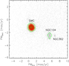 |
Fig. 3. Diagram showing PMRA vs. PMDec, in which the separation of selected SMC members (red), NGC 104 and NGC 362, is clearly shown. Based on this diagram, we estimate the contamination of remaining foreground sources for the SMC to be around 0.2% (∼98/45 466), which can be ignored. Green contours represent the number density. |
We note that the strict constraints on the astrometric solution and the previous deblending procedure may cause target loss and incompleteness in our catalog to a certain extent, but ensure that we select the true SMC targets. This can also be seen from the histogram of Gaia RVs in Fig. 4, where the separation of Milky Way and SMC is clear, and the vast majority of astrometry constrained targets with Gaia RVs larger than ∼90 km s−1 are selected with minimal value of ∼95 km s−1 (targets with both large PMs and RVs are not necessarily members of the SMC, as they could be hypervelocity stars in the Milky Way, runaway stars from the Milky Way or the SMC, or free-floating stars between the Milky Way and the SMC). Figure 5 illustrates the Gaia color-magnitude diagram (CMD) before (gray) and after (red) applying the astrometric constraints, where the large amount of foreground contamination of bright yellow and faint red stars is swept out. In addition, further constraints on the SEIP data, for example S/N ≥ 3 for IRAC1 (i1_fluxtype = 1), were investigated and resulted in a difference of only about 1.66% in the total number of sources (45 466 vs. 44 712 targets), and were therefore ignored.
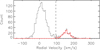 |
Fig. 4. RVs from Gaia. The separation of the Milky Way and the SMC is clear, and the vast majority of targets with RVs larger than ∼90 km s−1 are selected (red) with minimal value of ∼95 km s−1 (dashed line). |
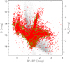 |
Fig. 5. Diagram showing G vs. BP − RP for the Gaia data before (gray) and after (red) the astrometric constraints, where the large number of foreground contamination is swept out. Green contours represent the number density. |
Based on this fiducial dataset of 45 466 targets, we retrieved additional optical and IR data from the following datasets with a search radius of 1″:
– 18 641 matches (41.00%) from the VISTA survey of the Magellanic Clouds system (VMC) DR4. The VMC is a NIR multi-epoch survey of the YJKS bands for the LMC, the SMC, and the MB (KS ≲ 20.3 mag, ∼2% photometric and ∼0.01″ astrometric precision), using the 4 m NIR optimized Visible and Infrared Survey Telescope for Astronomy (VISTA; Cioni et al. 2011).
– 28 678 matches (63.08%) from the IRSF Magellanic Clouds point source catalog (MCPS). The IRSF MCPS is a NIR photometric catalog of the JHKS bands for a 40 deg2 area in the LMC, an 11 deg2 area in the SMC, and a 4 deg2 area in the MB (KS ≲ 16.6 mag, photometric and astrometric accuracies for bright sources are 0.03−0.04 mag and 0.1″, respectively), based on data from the Simultaneous three-color InfraRed Imager for Unbiased Survey (SIRIUS) camera on the InfraRed Survey Facility (IRSF) 1.4 m telescope (Kato et al. 2007).
– 625 matches (1.37%) from AKARI SMC bright point source list, which represents NIR to MIR imaging and spectroscopic observations of patchy areas in the SMC (N3 ≲ 16.5 mag, ∼0.1 mag photometric and ≲0.8″ astrometric precision), using the Infrared Camera (IRC) aboard AKARI space telescope (Onaka et al. 2007; Murakami et al. 2007; Ita et al. 2010).
– Four matches from HERschel Inventory of the Agents of Galaxy Evolution (HERITAGE) band-merged source catalog (units are in flux [mJy] instead of magnitude). HERITAGE catalog is derived based on data from both Photodetector Array Camera and Spectrometer (PACS; 100 and 160 μm) and Spectral and Photometric Imaging Receiver (SPIRE; 250, 350, and 500 μm) cameras on board the Herschel Space Observatory, used to identify dusty objects in the LMC and SMC (the catalog also includes the Spitzer MIPS 70 μm band data, and none of our targets have been detected in the SPIRE 500 μm band; Pilbratt et al. 2010; Meixner et al. 2013; Seale et al. 2014).
– 40 387 matches (88.83%) from SkyMapper DR1.1 (we apply constraints on the parameters as flags < 4, nch_max = 1, nimaflags = 0 and class_star ≥ 0.9 to retrieve the data; see Wolf et al. 2018 for details). SkyMapper is a southern-hemisphere photometric survey in six bands (u, v, g, r, i, z; from magnitude 8 to 18, ∼1% photometric and < 0.2″ astrometric precision), using the dedicated 1.3 m SkyMapper telescope (Keller et al. 2007; Bessell et al. 2011; Wolf et al. 2018).
– 38 759 matches (85.25%) from the NOAO source catalog (NSC) DR1 (we apply constraints on the parameters, such as flags < 4 and class_star ≥ 0.9, to retrieve the data; see Nidever et al. 2018 for details). The NSC is a catalog of sources from most of the public data collected using the NOAO CTIO-4m+Decam as well as KPNO-4m+Mosaic3 (in u, g, r, i, z, Y bands, reaching ∼23 mag in most broadband filters with ∼1−2% photometric precision, and astrometric accuracy of ∼7 mas; Nidever et al. 2018).
– 11 630 matches (25.58%) from a UBVR CCD survey of the Magellanic Clouds by Massey (2002) (M2002; we note that due to some extremely large errors in the catalog, we replace those errors, e.g., > 1.0 mag, with NULL values). M2002 is a survey of 14.5 deg2 region in the LMC and 7.2 deg2 region in the SMC (V ≲ 18.0 mag, < 3% photometric and ∼0.3″ astrometric precision), using 0.61 m Curtis Schmidt telescope at CTIO.
– 164 matches (0.36%) from revised GALEX source catalog for the All-Sky Imaging Survey (GUVcat_AIS). GUVcat_AIS is a science-enhanced, “clean” catalog of GALEX UV sources with typical depths of 20.8 and 19.9 mag and position accuracies of 0.32″ and 0.34″ in NUV and FUV bands, respectively (Morrissey et al. 2007; Bianchi et al. 2017).
All the datasets are also deblended with a search radius of 3″ prior to crossmatching with the SEIP-Gaia dataset. Figure 6 shows the normalized transmission curves of all filters used in our study. In total, we have 50 filters including 21 optical (including the two UV filters) and 29 IR filters. The spatial distributions of the additional optical (left) and IR (right) datasets are shown in Fig. 7. The GALEX and HERITAGE data are not shown in the diagram due to the paucity of matches.
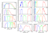 |
Fig. 6. Normalized transmission curves of filters (convolved with the instrument/telescope sensitivities) used in our study. In total, we have 50 filters including 21 optical (includes the two UV filters) and 29 IR filters. For each dataset, the filters are color coded from shorter (blueish) to longer (reddish) wavelengths. Left panel from top to bottom: BP, RP, and G from Gaia, U, B, V, and R from M2002, u, v, g, r, i, and z from SkyMapper, and u, g, r, i, z, and Y from NSC. Middle panel from top to bottom: J, H, KS from 2MASS, Y, J, KS from VMC, J, H, KS from IRSF, and FUV and NUV from GALEX. Right panel from top to bottom: IRAC1, IRAC2, IRAC3, IRAC4, and MIPS24 from Spitzer, WISE1, WISE2, WISE3, and WISE4 from WISE, N3, N4, S7, S11, L15, and L24 from AKARI, and MIPS70 (from Spitzer), PACS100, PACS160, SPIRE250, and SPIRE350 from Herschel. |
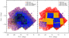 |
Fig. 7. Spatial distribution of the additional optical (left) and IR (right) datasets. The GALEX and HERITAGE data are not shown in the diagram due to the paucity of matches. Green contours represent the number density. |
In addition to the photometric data, additional classifications were also retrieved from the literature with a search radius of 1″, including:
– 37 375 matches from Boyer et al. (2011) (IR color classifications). This was an investigation of the IR properties of cool, evolved stars in the SMC, including the red giant branch (RGB) stars and the dust-producing red supergiant (RSG) and asymptotic giant branch (AGB) stars using observations from the Spitzer Space Telescope Legacy Program entitled “Surveying the Agents of Galaxy Evolution in the Tidally Stripped, Low Metallicity SMC (SAGE-SMC)”.
– 30 matches from Sewiło et al. (2013) (IR color and spectral energy distribution [SED] classifications). These authors used CMDs based on the multiwavelength photometric data and SED fitting to identify a population of approximately 1000 intermediate- to high-mass young stellar objects (YSOs) in the SMC.
– 43 matches from Ruffle et al. (2015) (MIR spectral classifications). These authors classified 209 point sources observed by Spitzer Infrared Spectrograph (IRS; Houck et al. 2004) using a decision tree method based on IR spectral features, continuum and SED shape, bolometric luminosity, cluster membership, and variability statistics (all the targets from Kraemer et al. 2017 were also included).
– 695 matches from Bonanos et al. (2010) (optical spectral classifications). This is a catalog of 5324 massive stars from the literature with accurate spectral types and a multiwavelength photometric catalog for a subset of 3654 of these stars in the SMC, intended for use in studying their IR properties.
– 198 matches from González-Fernández et al. (2015) (spectral variability flag, radial velocities, and optical spectral classifications; for convenience, we only kept the first spectral classification for targets with multiple measurements). These authors studied physical properties of about 500 RSGs in the LMC and SMC using NIR/MIR photometry and optical spectroscopy, aiming at exploring the fainter end of RSGs and extrapolating their behavior to other environments by building a more representative sample.
– 113 matches from Neugent et al. (2018) (data originated from Neugent et al. 2010; radial velocities and optical spectral classifications). Neugent et al. (2018) spectroscopically observed 176 near-certain (Category 1) SMC yellow supergiant stars (YSGs) among approximately 500 candidates to test against the evolutionary model in the low-metallicity environment.
– 39 295 matches from Simbad (Wenger et al. 2000). The radial velocities, optical spectral classifications, main object types, and auxiliary object types were retrieved.
The unmatched targets are likely due to larger PMs, blends, or the quality cuts in SEIP or Gaia catalog.
This multiwavelength source catalog with 45 466 targets serves as the backbone of our study. The sample consists of “bona-fide” and “dusty” SMC targets determined by both astrometric measurement and IR detection. Table 1 shows the absolute and relative percentage (relative to the filter with the most matches in each dataset) of detected targets in each filter. Figure 8 shows the histograms of magnitude distribution for each dataset (for convenience, the HERITAGE data are not shown here). The bin size is 0.1 mag, except for the GALEX (0.5 mag) and AKARI (0.25 mag) data. For WISE3 and WISE4 bands, due to the fact that the majority of the targets (∼75% in WISE3 and ∼95% in WISE4 bands) have low S/N (< 2) and are derived with a 95% confidence brightness upper limit, the histograms only show targets with S/N ≥ 2.
Number of detected targets in each filter of the SMC source catalog.
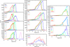 |
Fig. 8. Histograms of magnitude distribution in each dataset. The bin size of magnitude is 0.1 mag, except for the GALEX (0.5 mag) and AKARI (0.25 mag) data. For WISE3 and WISE4 bands, the histograms only show targets with S/N ≥ 2. For convenience, the HERITAGE data are not shown in the diagram. |
3. Multiwavelength time-series data
Following Yang et al. (2018), the MIR time-series data of WISE1 (3.4 μm) and WISE2 (4.6 μm) bands for all 45 466 targets were collected from both ALLWISE (Cutri et al. 2013) and Near-Earth Object WISE Reactivation mission (NEOWISE-R; Mainzer et al. 2014), with a search radius of 1″ and the following parameter constraints: qi_fact > 0, saa_sep > 0, moon_masked = 0, qual_frame > 0, det_bit = 3, and χ2 ≤ 10, S/N ≥ 3 (see Yang et al. 2018 for details), which resulted in about 2.28 million measurements from ALLWISE and 8.78 million measurements from NEOWISE-R. With the NEOWISE 2019 data release, the total frame coverage is about twelve major epochs spanning about 3200 days (∼8.8 years) with two epochs from ALLWISE and ten epochs from NEOWISE-R separated by an approximately three-year gap. The beginning and end of each epoch set by us is given in Table 2. We binned the data within each epoch by using the median values of the date and magnitudes. For each epoch, we required at least five valid points to calculate the median value. Figure 9 shows examples of the original light curves overlapped with the binned light curves. The median absolute deviation (MAD) and standard deviation (SD) were used to calculate the long-term (full light curve) and short-term (within single epoch) variability of each target with at least five valid points, where the former was more resistant to outliers than the latter (Rousseeuw & Croux 1993). Although it is possible to derive periods based on the current data, the period search may be highly contaminated by the strong alias structures due to the very low sampling of WISE data as shown in Fig. 9; we only have twelve epochs spanning ∼3200 days and each epoch only covers about 5 to 10 days (we refer interested readers to Chen et al. 2018 for the WISE catalog of periodic variable stars). In addition to MAD and SD, the full amplitude (Amp = maxmag − minmag) was also calculated for each target. More details about the WISE time-series data reduction can be found in Yang et al. (2018). In total, there are 39 694 (87.30%) targets with variability statistics in both WISE1 and WISE2 bands covering almost the whole area of our sample. The lack of variability statistics for some targets is likely due to either faint magnitudes or the quality cuts we adopted.
Observation epochs of ALLWISE and NEOWISE-R.
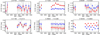 |
Fig. 9. Examples of original (light gray for WISE1 and dark gray for WISE2) and binned (blue for WISE1 and red for WISE2) light curves. There are about twelve major epochs with two epochs from ALLWISE (open circles) and ten epochs from NEOWISE-R (open squares) separated by an approximately three-year gap. Coordinates of the targets are indicated on top of each panel. |
In addition to the WISE data, we also collected other sets of variability data from different projects, including IR data from the SAGE-Var program (Riebel et al. 2015), VMC, and IRSF, and optical data from Gaia, NSC, and OGLE. SAGE-Var is a follow-up to the Spitzer legacy program SAGE (Meixner et al. 2006; Gordon et al. 2011), where six total epochs of photometric observations at IRAC1 (3.6 μm) and IRAC2 (4.5 μm) bands were obtained covering the bar of the LMC and the central region of the SMC with 15 different timescales ranging from ∼20 d to ∼5 yr. We collected the SMC data and calculated the median magnitudes, MADs, SDs, and Amps for targets with all six epochs available. In total, there are 7160 (15.75%) targets in IRAC1 band and 5894 (12.96%) targets in IRAC2 band matched with our source catalog within 1″. The left panel of Fig. 10 shows the spatial distribution of those targets overlapped on our source catalog.
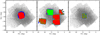 |
Fig. 10. Spatial distribution of targets with IR variability statistics matched with our source catalog within 1″. Left: targets from SAGE-Var project, where blue and red colors indicate the targets in IRAC1 and IRAC2 bands, respectively. Middle: targets from VMC DR4, where blue, green, and red colors indicate the targets in Y, J, and KS bands, respectively. Right: targets from IRSF survey, where blue, green, and red colors indicate the targets in J, H, and KS bands, respectively. |
We currently rely on the available information from VMC DR4 regarding the variability statistics, as the final release (which may also include the time-series data) with global photometric and astrometric calibration will be made available upon completion of the survey2. Since the observational cadences for different targets and filters were irregular and the median values of cadences varied from a few hours to hundreds of days, for each filter we constrained all the values of median magnitudes, MADs, SDs, and Amps to be within the range of 0 to 99 with at least five good measurements (nGoodObs ≥ 5) to avoid any unphysical values. In total, there are 11 197 (24.63%) targets matched with our source catalog within 1″ as shown in the middle panel of Fig. 10. There are 11 197 (24.63%) targets in Y band, 11 125 (24.47%) targets in J band, and 7574 (16.66%) targets in KS band. Additionally, there are 204 targets that were classified as Cepheids by the VMC team matched with our source catalog within 1″.
For IRSF data, we retrieved the time-series data of approximately 1000 targets for each filter from Ita et al. (2018), where a very long-term (2000−2017) NIR-variable star survey towards an area of 3 deg2 along the bar in the LMC and an area of 1 deg2 in the central part of the SMC was carried out with more than 100 repeated observations for each area. The median magnitudes, MADs, SDs, and Amps were calculated for each target. There are 160 targets in J band, 161 targets in H band, and 154 targets in KS band matched with our source catalog within 1″ as shown in the right panel of Fig. 10.
Gaia DR2 provides classifications for more than 550 000 variable sources consisting of different types of variables. However, only a subset of the variable stars classified as a certain type are characterized in detail and a fraction of the classifications may well be incorrect (Gaia Collaboration 2019; Mowlavi et al. 2018). Since the time-series data will be provided in a future release, we retrieved the variability statistics (including MADs, SDs, and Amps) and classifications from the Gaia archive3 with typically approximately 30 measurements spanning ∼620 days. However, we note that the MAD is scaled by 1.4826, meaning that the expectation of the scaled MAD at large number of measurements is equal to the standard deviation of a normal distribution4. For consistency of the dataset, we reversed the scaled MAD by dividing it by 1.4826. There are 1379 (3.03%; blue) targets with variability statistics which are matched with our source catalog within 1″ as shown in the left panel of Fig. 11, while 1277 (2.81%; orange) of them are classified, and 868 (1.91%; red) of them have best_class_score ≥ 0.5 (best_class_score is a quantity between 0 and 1 provided by the classification pipeline to estimate the confidence of the classifier in the identification of various variability types), for which the classification may be acceptable.
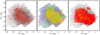 |
Fig. 11. Spatial distribution of targets with optical variability statistics matched with our source catalog within 1″. Left: targets from Gaia, where blue, orange, and red colors indicate targets without classification, with best_class_score < 0.5, and best_class_score ≥ 0.5, respectively. Middle: targets from NSC, where violet, blue, cyan, green, orange, and red colors indicate the targets in u, g, r, i, z, and Y bands, respectively. Right: targets from OGLE, where blue, green, orange, and red colors indicate the targets classified as Ecls, T2Ceps, CCeps, and LPVs, respectively. |
The NSC time-series data for the SMC are mainly from the Survey of the Magellanic Stellar History (SMASH; Nidever et al. 2017). We retrieved the data from the NOAO Data Lab5 with the same sky coverage and constraint parameters (flags < 4 and class_star ≥ 0.9). By crossmatching with our source catalog using a search radius of 1″, we retrieved 132 342 measurements in u-band, 355 823 measurements in g-band, 497 443 measurements in r-band, 210 496 measurements in i-band, 404 087 measurements in z-band, and 16 916 measurements in Y-band. However, due to the irregular sampling in different filters, the observational timescales vary from tenths of a day to more than 1000 days, with several to hundreds of measurements. Thus, we required at least five valid measurements for each target in individual filters in order to calculate the MAD, SD, and Amp. We must emphasize that as a result of the irregular sampling, and in particular a strong systematic effect that we discovered during the data processing (instead of a relatively uniform distribution, different SMC regions show variable levels of average variabilities), the calculated variability may not fully represent the true variability of the target and the user should be cautious when using these values. The middle panel of Fig. 11 shows the spatial distribution of targets with variability statistics in different filters, including 17 548 (38.60%) targets in u-band, 25 897 (57.00%) targets in g-band, 29 572 (65.04%) targets in r-band, 19 632 (43.18%) targets in i-band, 35 850 (78.85%) targets in z-band, and 1212 (2.67%) targets in Y-band.
Finally, we obtained additional data from the Optical Gravitational Lensing Experiment (OGLE; Udalski et al. 1992, 2008, 2015; Szymanski 2005) using a search radius of 1″ from both the OGLE-III Catalog of Variable Stars (O3CVS) and the OGLE-IV Collection of Variable Stars (O4CVS), which resulted in 8956 (19.70%) long-period variables (LPVs) from O3CVS, and 482 (1.06%) classical Cepheids (CCeps), 11 (0.02%) Type II Cepheids (T2Ceps), and 87 (0.19%) eclipsing binaries (Ecls) from O4CVS (Soszyński et al. 2011, 2015, 2018; Pawlak et al. 2016) as shown in the right panel of Fig. 11. However, since the OGLE data are calculated using Fourier analysis, which is different from our dataset, only the classifications are used in the further analysis. Figure 12 shows Gaia CMDs with variable classifications from Gaia (left; only shows targets with best_class_score ≥ 0.5), OGLE (middle), and VMC (right).
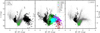 |
Fig. 12. Gaia CMDs with variable classifications from Gaia (left), OGLE (middle), and VMC (right). Left panel: only shows targets with best_class_score ≥ 0.5 from Gaia. Green contours represent the number density. |
We also checked the time-series data from SkyMapper DR1.1. However, this first data release provides only a few measurements (∼1−2) covering ∼300 days and is not suitable for robust variability calculation. Our SMC source catalog of 45 466 targets is available in its entirety in CDS. Table 3 documents the columns found in the catalog. Targets without errors indicate either a 95% confidence upper limit, or the errors are simply too large to be reliable (e.g., > 1.0 mag).
Contents of the SMC source catalog.
4. Identifying evolved massive star candidates on the CMDs
As we focus on the evolved dusty massive stars, the primary task is to identify them. We utilize the evolutionary tracks and synthetic photometry from Modules for Experiments in Stellar Astrophysics (MESA; Paxton et al. 2011, 2013, 2015, 2018) Isochrones & Stellar Tracks (MIST6; Choi et al. 2016; Dotter 2016), which covers a wide range of ages, masses, and metallicities using solar-scaled abundance under a single computational framework to identify evolved massive star candidates on the CMDs of our multiwavelength source catalog.
We used a canonical value of 18.95 as the distance modulus of the SMC (Graczyk et al. 2014; Scowcroft et al. 2016). Since the metallicity of the SMC is about 10 to 20% solar (Russell & Dopita 1992; Dobbie et al. 2014; D’Onghia & Fox 2016), we adopted the chemical composition of −1.0 to −0.7 dex for [Fe/H]. The nonrotation and rotation (V/Vcrit = 0.40) models of 7 to 40 M⊙ were computed with no extinction and extinction of AV = 1.0 mag, respectively (Cardelli et al. 1989; Zaritsky et al. 2002; Haschke et al. 2011; Gao et al. 2013). We chose the color-magnitude combinations based on the available synthetic photometry in MIST with relative percentage > 90% (see Table 1) at longer wavelengths (some dusty massive stars might not be identified in the shorter wavelengths due to higher extinction and reddening). The Yellow Void between blue supergiant stars (BSGs) and RSGs were also clearly shown in those models in order to identify YSGs.
Figure 13 shows multiple optical CMDs of Gaia, SkyMapper, NSC, and M2002 datasets overlapped with the evolutionary tracks of 7, 9, 12, 15, 20, 25, 32, and 40 M⊙ generated from MIST synthetic photometry. The tracks are color-coded based on the equivalent evolutionary phases (EEPs) from core helium burning to carbon burning, and Teff of 7500 K < Teff (blue; BSGs), 5000 < Teff ≤ 7000 K (yellow; YSGs), and Teff ≤ 5000 K (red; RSGs) (Neugent et al. 2010). The regions of each type of evolved massive star are outlined by the dashed lines with color and magnitude criteria listed in Table 4. Due to the relatively large MLR during the RSG phase, the star could be heavily obscured by the surrounding dust envelope (Smith et al. 2001; Massey et al. 2005; Levesque et al. 2006; Yang et al. 2018; Ren et al. 2019). Therefore, we also empirically extended the RSG region from the reddest and faintest points of the models to the even redder but not fainter area in order to avoid the contamination from extreme AGBs (x-AGB stars are most likely experiencing a “superwind”, where the MLR can increase by a factor of ten, and a thick dust envelope obscures the star at optical wavelengths; van Loon et al. 2006; Boyer et al. 2011) as shown in the diagrams. It may be that some super-AGBs (stars in the mass range of ∼7 − 10 M⊙ that represent a transition to the more massive supergiant stars and are characterized by degenerate off-centre carbon ignition analogous to the earlier helium flash; Herwig 2005; Siess 2006, 2007, 2010; Groenewegen et al. 2009; Doherty et al. 2017) are also selected by the extension. However, we expect them to be rejected by the use of several methods as shown in Yang et al. (2018). Moreover, inevitably there will be contamination of the main sequence massive stars at the blue end, which cannot be easily disentangled. The diagrams show a clear bimodal distribution of the BSG and RSG candidates with a few YSG candidates lying between them. We notice that the conventional lower limit of the stellar mass for “massive stars” is usually defined as eight solar masses. However, our initial tests show that the observational data are fitted better with the evolutionary track of seven solar masses (or even lower) as shown in the diagrams. This may be due to the treatment of parameters in the model such as convective overshooting, rotation, mixing, metallicity, and MLR, or the uncertainties of extinction and/or bolometric correction, or it may be true that massive stars have a lower limit of stellar mass, which is complicated and requires further investigation.
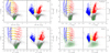 |
Fig. 13. Color-magnitude diagrams of Gaia (upper left), SkyMapper (upper right), NSC (bottom left), and M2002 (bottom right) datasets. In each diagram, left panel: CMD overlapped with MIST evolutionary tracks of 7, 9, 12, 15, 20, 25, 32 and 40 M⊙ and color-coded as BSG (blue), YSG (yellow), and RSG (red) phases. The regions of each type of evolved massive star are outlined by the dashed lines. Targets without errors are not shown in the CMDs, while the average photometric uncertainties are indicated when available. Right panel: selected targets for each type of massive stars with the same color convention. The RSG region is empirically extended as shown by the horizontal dashed lines. Green contours represent the number density. See text for details. |
Evolved massive star candidate selection criteria.
It can be seen from Fig. 13 that in the optical bands, massive stars generally evolve horizontally across the upper part of CMD, while it is slightly different in the NIR bands. The left panel of Fig. 14 shows the 2MASS CMD overlapped with MIST tracks, for which the tracks extend from the fainter and bluer region to the brighter and redder area due to the displacement of Teff and intrinsic emission peaks. The right panel of Fig. 14 shows a different method to classify RSGs originating from Cioni et al. (2006a) and Boyer et al. (2011) (hereafter CB method), where oxygen-rich AGBs (O-AGBs) are defined by KS < KS-band tip of the red giant branch (KS-TRGB ≈ 12.7 mag) and K1 < J − KS < K2, carbon-rich AGBs (C-AGBs) are defined by KS < KS-TRGB and K2 < J − KS < 2.1 mag, x-AGBs are defined by J − KS > 2.1 mag (all AGB stars are brighter than the K0 line, except x-AGBs), and RSGs are defined by Δ(J − KS) = 0.25 mag from the O-AGBs shown as the dashed line in the diagram (the distance and 0.05 mag for the metallicity between LMC and SMC are corrected; Cioni et al. 2006b). It occurs to us that the CB method covers almost the whole magnitude range of the RSG population down to the KS-TRGB, which cannot be covered by the MIST tracks. However, MIST tracks are more broadened with a part of the tracks also extending to the O-AGBs region. This discrepancy between MIST tracks and the CB method will be addressed in our next paper. A simple calculation using a constant bolometric correction (BC) of BCKS = 2.69 (Davies et al. 2013) and AKS = 0.1 mag shows that the RSG candidates close to KS-TRGB (e.g., KS = 12.6 mag) only correspond to ∼103.4 (∼2500) solar luminosity (L⊙).
 |
Fig. 14. Diagram showing KS vs. J − KS for the 2MASS dataset. Left panel: similar to Fig. 13 as massive star candidates selected by MIST tracks. Right panel: definitions of C-AGB, O-AGB, x-AGB, and RSG regions based on theoretical J − KS color cuts from Cioni et al. (2006a) and Boyer et al. (2011). Targets selected as RSG candidates are shown in red. Green contours represent the number density. |
We also notice one important observational piece of evidence: for the RSGs population, there is a distinct branch stretching continuously from the top of the luminous cool region towards the relatively faint warm area, reaching approximately the TRGB without blending into the AGBs population. This is clearly beyond the limit of the 7 M⊙ track and most probably reaches down to 6 M⊙. False detection is ruled out for two reasons: First, all the Gaia, SkyMapper, NSC, and 2MASS data show the same tendency except the M2002 data, which is likely due to the photometric sensitivity. Second, our sample is strictly constrained by the Gaia astrometric solution and verified by comparing with the results of Gaia Collaboration (2018b), which indicate that the luminosities and colors of our targets are almost certain and the photometric errors are also very small at the magnitude range around the TRGB. Figure 15 shows the zoomed-in regions of 0.8 < BP − RP < 2.5 and 14.0 < G < 18.0 for Gaia (upper left), 0 < r − i < 1.2 and 13.5 < i < 17.5 for SkyMapper (upper right), 0.3 < g − r < 2.0 and 14.0 < r < 18.0 for NSC (bottom left), and 0.3 < J − KS < 1.5 and 10.5 < KS < 15.5 for 2MASS (bottom right). From the diagram and the observational point of view, there is no doubt that the separation between the RSG and AGB populations is relatively clear, even at faint magnitude. Additionally, the distribution of a large sample of spectroscopic SMC RSGs (more than 300 and brighter than KS ≈ 11.0 mag) on the 2MASS CMD follows almost exactly the MIST tracks, indicating the excellence of the MIST model prediction (details will be presented in our next paper). Therefore, even though there may still be inevitable contamination of AGBs at the faint magnitude end of the RSG sample, we do believe that it should be small, and will be easily resolved by the next generation of large-scale spectroscopic surveys (e.g., 4MOST, MOONS; Cirasuolo et al. 2012; de Jong et al. 2012). Despite the small amount of contamination, the overlapping of lower (initial) masses of RSGs and the upper limits of AGBs, and the clear separation between them at faint magnitude range, are also very interesting and puzzling. These results suggest that, at given magnitude, some stars evolve to RSGs and the others evolve to AGBs. Currently, we have no certain explanation for this. It may be due to the rotation, binarity, chemical composition, MLR, or even more sophisticated evolution. Nevertheless, this result may indicate the uniqueness of the RSG population, which connects the evolved massive and intermediate stars, since stars with initial masses of around 6 to 8 M⊙ are thought to go through a second dredge-up to become AGBs (Eldridge et al. 2007). The low-mass RSGs may also be related to the intermediate-luminosity optical transients (ILOTs; Prieto et al. 2008; Bond et al. 2009; Berger et al. 2009). Still, more investigations are needed to confirm the true nature of RSGs.
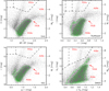 |
Fig. 15. Zoomed-in regions of 0.8 < BP − RP < 2.5 and 14.0 < G < 18.0 for Gaia (upper left), 0 < r − i < 1.2 and 13.5 < i < 17.5 for SkyMapper (upper right), 0.3 < g − r < 2.0 and 14.0 < r < 18.0 for NSC (bottom left), and 0.3 < J − KS < 1.5 and 10.5 < KS < 15.5 for 2MASS (bottom right). The populations of RSGs, AGBs, RGBs, and the TRGB are indicated on the diagram. It can be seen that the separation between the RSG and AGB populations is relatively clear, even at faint magnitude. |
We combined the candidates of each type of evolved massive star from different datasets and removed the duplications, which resulted in 1405 RSG, 217 YSG and 1369 BSG candidates listed in Table 5. Since the candidates were mostly selected based on the MIST model prediction in different datasets with a variety of filters, sky coverage, photometric sensitivities, and qualities, it was difficult to judge the reliability of the candidacies. Therefore, we ranked (Rank 0 to 5) the candidates based on the intersection between different CMDs, where Rank 0 indicated that a target was identified as the same type of evolved massive star in all five datasets (Gaia, SkyMapper, NSC, M2002 and 2MASS) by the MIST models and so on, and Rank 5 indicated the additional RSG candidates identified by the CB method but not recovered by the MIST models. Table 6 shows the numbers of ranked candidates for each type of evolved massive star.
Numbers of identified evolved massive star candidates.
Numbers of ranked evolved massive star candidates.
Figure 16 illustrates two CMDs (Gaia and 2MASS) for all the candidates with ranks, where RSG, YSG, and BSG candidates are color-coded in red, yellow, and blue ranging from dark (Rank 0) to light (Rank 5). Detailed information about each type of evolved massive star candidate is presented in separate tables available in the CDS with similar formats to that of Table 3, except the Rank has been added as an additional column at the end of each table. It must be emphasized that some candidates may have more than one classification, which is likely due to either the inevitable slight overlap of adjacent types of massive stars, or the larger uncertainties of photometry at the fainter magnitudes. Moreover, there are very few stray candidates located inside the regions of other populations deserved to be investigated. For example, a couple of BSG candidates appearing in the RSG region in the 2MASS CMD are likely there due to their thick circumstellar dust envelope, since they are also very bright in the MIR bands. Similarly, we notice that there are a few RSG candidates scattered in the much fainter and redder regions in the Gaia CMD. However, simultaneous inspection of the optical and MIR CMDs shows that almost all the scattered candidates in the bottom right region show IR excess and/or high MIR luminosity, which may indicate that the dimming in the optical band is caused by the circumstellar dust envelope. Finally, Fig. 17 shows the spatial distribution of evolved massive star candidates. It is clearly shown that due to the interaction between LMC and SMC, a number of candidates are stretched towards the MB. These populations follow the distribution of star formation in the SMC, which is predominantly along the bar of the SMC, and extend to the LMC through the MB. This is depicted from the star cluster (especially for those with ages < 100 Myr) distribution of the SMC (Bitsakis et al. 2018). A further detailed analysis of identified massive star populations will be presented in our following papers.
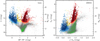 |
Fig. 16. Color-magnitude diagrams of Gaia (left) and 2MASS (right) with RSG (red), YSG (yellow), and BSG (blue) candidates overlapping, where the colors are coded from dark (Rank 0) to light (Rank 5) based on the ranks. The RSG branch extends towards fainter magnitudes with a few candidates scattered in the much fainter and redder region in the optical band, which is likely caused by the circumstellar dust envelope. Green contours represent the number density. |
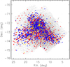 |
Fig. 17. Spatial distribution of evolved massive star candidates. Due to the interaction between LMC and SMC, a number of candidates are stretched towards the MB. |
Finally, we would like to emphasize again one important point: our purpose was to study the evolved dusty massive stars in the SMC by identifying BSG, YSG, and RSG populations primarily based on IR detections, and constrained by the astrometric solutions and the evolutionary models. In that sense our sample is incomplete due to the strict constraints on the astrometry, deblending, limitations of the models, and more importantly, the (presumably) serious differences in the luminosity completeness limits as a function of temperature. As we adopted the magnitude cut at the MIR wavelength (IRAC1 or WISE1 ≤ 15.0 mag), hotter stars would suffer more from incompleteness due to the weaker radiation at the far end of the Rayleigh-Jeans tail than the cooler stars. Even for the hot stars themselves, the degeneracy in the IR detection would occur for hotter stars with larger MLRs (less contribution from the stellar emission and more contribution from the dust emission) and cooler stars with smaller MLRs (vice versa), since they might have similar radiative intensities at the same MIR wavelengths, which also happens in all magnitude ranges (not to mention the MLR caused by binarity). One should not simply conclude that the BSG to RSG ratio (B/R ratio) is about 1:1 in the SMC, since both observation and theoretical prediction indicate that there will be more BSGs than RSGs (e.g., B/R ratio ∼4 or more) in the SMC (Meylan & Maeder 1982; Humphreys & McElroy 1984; Guo & Li 2002).
5. Summary
We present a clean, magnitude-limited (IRAC1 or WISE1 ≤ 15.0 mag) multiwavelength source catalog for the SMC with 45 466 targets in total. We intend to build our catalog as a comprehensive dataset serving as an anchor for future studies, especially for massive star populations at low metallicity. The catalog contains data in 50 different bands including 21 optical and 29 IR bands, retrieved from SEIP, VMC, IRSF, AKARI, HERITAGE, Gaia, SkyMapper, NSC, M2002, and GALEX datasets, ranging from UV to FIR. Additionally, RVs and spectral classifications were collected from the literature, as well as the IR variability statistics, including MAD, SD, and Amp derived from WISE, SAGE-Var, VMC, and IRSF, and the optical variability statistics derived from Gaia, NSC, and OGLE.
The catalog was essentially built upon a 1″ crossmatching and a 3″ deblending between SEIP source list and Gaia photometric data. We further constrained the PMs and parallaxes from Gaia DR2 to remove the foreground contamination, by applying a Gaussian profile in parallax with an additional elliptical constraint derived from PMRA and PMDec. We estimated that about 99.5% of the targets in our catalog were most likely genuine members of the SMC.
By using the evolutionary tracks and synthetic photometry from MIST and also the theoretical J − KS color cuts from CB method, we identified three evolved massive star populations in the SMC, namely the BSGs, YSGs, and RSGs, in five different CMDs. There are 1405 RSG, 217 YSG, and 1369 BSG candidates, respectively. We emphasized that our sample was incomplete for several reasons. We ranked the candidates based on the intersection of different CMDs, where the source with the most intersections was given the highest rank. A comparison between the models and observational data shows that the lower limit of initial mass for the RSG population may reach down to 7 or even 6 M⊙ and that the RSG is well separated from the AGB population even at faint magnitude, making RSGs a unique population connecting the evolved massive and intermediate stars, since stars with initial masses of around 6 to 8 M⊙ are thought to go through a second dredge-up to become AGBs.
We encourage the interested reader to further exploit the potential of our catalog, including but not limited to massive stars, SN progenitors, star formation history, stellar population, stellar kinematics, chemical evolution, individual and integrated SED, time-domain astronomy, and so on. A further detailed analysis of the RSG population in the SMC will be presented in our next paper.
Acknowledgments
We would like to thank the anonymous referee for many constructive comments and suggestions. We acknowledge funding from the European Research Council (ERC) under the European Union’s Horizon 2020 research and innovation programme (grant agreement number 772086), and from Hubble Catalog of Variables project funded by the European Space Agency (ESA) under contract No.4000112940. B.W.J. and J.G. gratefully acknowledge support from the National Natural Science Foundation of China (Grant No.11533002 and U1631104). We thank Man I Lam and Stephen A.S. de Wit for helpful comments and suggestions. This publication makes use of data products from the Two Micron All Sky Survey, which is a joint project of the University of Massachusetts and the Infrared Processing and Analysis Center/California Institute of Technology, funded by the National Aeronautics and Space Administration and the National Science Foundation. This work is based in part on observations made with the Spitzer Space Telescope, which is operated by the Jet Propulsion Laboratory, California Institute of Technology under a contract with NASA. This publication makes use of data products from the Wide-field Infrared Survey Explorer, which is a joint project of the University of California, Los Angeles, and the Jet Propulsion Laboratory/California Institute of Technology. It is funded by the National Aeronautics and Space Administration. This publication makes use of data products from the Near-Earth Object Wide-field Infrared Survey Explorer (NEOWISE), which is a project of the Jet Propulsion Laboratory/California Institute of Technology. NEOWISE is funded by the National Aeronautics and Space Administration. This research has made use of the NASA/IPAC Infrared Science Archive, which is operated by the Jet Propulsion Laboratory, California Institute of Technology, under contract with the National Aeronautics and Space Administration. This work has made use of data from the European Space Agency (ESA) mission Gaia (https://www.cosmos.esa.int/gaia), processed by the Gaia Data Processing and Analysis Consortium (DPAC, https://www.cosmos.esa.int/web/gaia/dpac/consortium). Funding for the DPAC has been provided by national institutions, in particular the institutions participating in the Gaia Multilateral Agreement. This research uses services or data provided by the NOAO Data Lab. NOAO is operated by the Association of Universities for Research in Astronomy (AURA), Inc. under a cooperative agreement with the National Science Foundation. The national facility capability for SkyMapper has been funded through ARC LIEF grant LE130100104 from the Australian Research Council, awarded to the University of Sydney, the Australian National University, Swinburne University of Technology, the University of Queensland, the University of Western Australia, the University of Melbourne, Curtin University of Technology, Monash University and the Australian Astronomical Observatory. SkyMapper is owned and operated by The Australian National University’s Research School of Astronomy and Astrophysics. The survey data were processed and provided by the SkyMapper Team at ANU. The SkyMapper node of the All-Sky Virtual Observatory (ASVO) is hosted at the National Computational Infrastructure (NCI). Development and support the SkyMapper node of the ASVO has been funded in part by Astronomy Australia Limited (AAL) and the Australian Government through the Commonwealth’s Education Investment Fund (EIF) and National Collaborative Research Infrastructure Strategy (NCRIS), particularly the National eResearch Collaboration Tools and Resources (NeCTAR) and the Australian National Data Service Projects (ANDS). This research has made use of the SIMBAD database and VizieR catalog access tool, operated at CDS, Strasbourg, France, and the Tool for OPerations on Catalogues And Tables (TOPCAT; Taylor 2005). Based on data products from observations made with ESO Telescopes at the La Silla or Paranal Observatories under ESO programme ID 179.B-2003.
References
- Aadland, E., Massey, P., Neugent, K. F., et al. 2018, AJ, 156, 294 [NASA ADS] [CrossRef] [Google Scholar]
- Arenou, F., Luri, X., Babusiaux, C., et al. 2018, A&A, 616, A17 [Google Scholar]
- Barba, R. H., Niemela, V. S., Baume, G., & Vazquez, R. A. 1995, ApJ, 446, L23 [CrossRef] [Google Scholar]
- Berger, E., Soderberg, A. M., Chevalier, R. A., et al. 2009, ApJ, 699, 1850 [NASA ADS] [CrossRef] [Google Scholar]
- Bessell, M., Bloxham, G., Schmidt, B., et al. 2011, PASP, 123, 789 [NASA ADS] [CrossRef] [Google Scholar]
- Bianchi, L., Shiao, B., & Thilker, D. 2017, ApJS, 230, 24 [NASA ADS] [CrossRef] [Google Scholar]
- Bitsakis, T., González-Lópezlira, R. A., Bonfini, P., et al. 2018, ApJ, 853, 104 [NASA ADS] [CrossRef] [Google Scholar]
- Bonanos, A. Z., Massa, D. L., Sewilo, M., et al. 2009, AJ, 138, 1003 [NASA ADS] [CrossRef] [Google Scholar]
- Bonanos, A. Z., Lennon, D. J., Köhlinger, F., et al. 2010, AJ, 140, 416 [NASA ADS] [CrossRef] [Google Scholar]
- Bond, H. E., Bedin, L. R., Bonanos, A. Z., et al. 2009, ApJ, 695, L154 [NASA ADS] [CrossRef] [Google Scholar]
- Bouret, J.-C., Lanz, T., Martins, F., et al. 2013, A&A, 555, A1 [NASA ADS] [CrossRef] [EDP Sciences] [Google Scholar]
- Boyer, M. L., Srinivasan, S., van Loon, J. T., et al. 2011, AJ, 142, 103 [Google Scholar]
- Britavskiy, N., Lennon, D. J., Patrick, L. R., et al. 2019, A&A, 624, A128 [NASA ADS] [CrossRef] [EDP Sciences] [Google Scholar]
- Bromm, V., Yoshida, N., Hernquist, L., et al. 2009, Nature, 459, 49 [NASA ADS] [CrossRef] [PubMed] [Google Scholar]
- Cardelli, J. A., Clayton, G. C., & Mathis, J. S. 1989, ApJ, 345, 245 [NASA ADS] [CrossRef] [Google Scholar]
- Castro, N., Oey, M. S., Fossati, L., & Langer, N. 2018, ApJ, 868, 57 [NASA ADS] [CrossRef] [Google Scholar]
- Chen, X., Wang, S., Deng, L., de Grijs, R., & Yang, M. 2018, ApJS, 237, 28 [NASA ADS] [CrossRef] [Google Scholar]
- Chiavassa, A., Pasquato, E., Jorissen, A., et al. 2011, A&A, 528, A120 [NASA ADS] [CrossRef] [EDP Sciences] [Google Scholar]
- Choi, J., Dotter, A., Conroy, C., et al. 2016, ApJ, 823, 102 [NASA ADS] [CrossRef] [Google Scholar]
- Cioni, M.-R. L., Girardi, L., Marigo, P., & Habing, H. J. 2006a, A&A, 448, 77 [NASA ADS] [CrossRef] [EDP Sciences] [Google Scholar]
- Cioni, M.-R. L., Girardi, L., Marigo, P., & Habing, H. J. 2006b, A&A, 452, 195 [NASA ADS] [CrossRef] [EDP Sciences] [Google Scholar]
- Cioni, M.-R. L., Clementini, G., Girardi, L., et al. 2011, A&A, 527, A116 [NASA ADS] [CrossRef] [EDP Sciences] [Google Scholar]
- Cirasuolo, M., Afonso, J., Bender, R., et al. 2012, Proc. SPIE, 8446, 84460S [NASA ADS] [CrossRef] [Google Scholar]
- Cutri, R. M., Wright, E. L., Conrow, T., et al. 2013, VizieR Online Data Catalog: II/328 [Google Scholar]
- Davies, B., Kudritzki, R.-P., Plez, B., et al. 2013, ApJ, 767, 3 [NASA ADS] [CrossRef] [Google Scholar]
- de Jong, R. S., Bellido-Tirado, O., Chiappini, C., et al. 2012, Proc. SPIE, 8446, 84460T [Google Scholar]
- Dobbie, P. D., Cole, A. A., Subramaniam, A., & Keller, S. 2014, MNRAS, 442, 1680 [NASA ADS] [CrossRef] [Google Scholar]
- Doherty, C. L., Gil-Pons, P., Siess, L., et al. 2017, PASA, 34, e056 [NASA ADS] [CrossRef] [Google Scholar]
- D’Onghia, E., & Fox, A. J. 2016, ARA&A, 54, 363 [NASA ADS] [CrossRef] [Google Scholar]
- Dotter, A. 2016, ApJS, 222, 8 [NASA ADS] [CrossRef] [Google Scholar]
- Eldridge, J. J., Mattila, S., & Smartt, S. J. 2007, MNRAS, 376, L52 [NASA ADS] [Google Scholar]
- Evans, C. J., & Howarth, I. D. 2008, MNRAS, 386, 826 [CrossRef] [Google Scholar]
- Gaia Collaboration (Prusti, T., et al.) 2016, A&A, 595, A1 [NASA ADS] [CrossRef] [EDP Sciences] [Google Scholar]
- Gaia Collaboration (Brown, A. G. A., et al.) 2018a, A&A, 616, A1 [NASA ADS] [CrossRef] [EDP Sciences] [Google Scholar]
- Gaia Collaboration (Helmi, A., et al.) 2018b, A&A, 616, A12 [NASA ADS] [CrossRef] [EDP Sciences] [Google Scholar]
- Gaia Collaboration (Eyer, L., et al.) 2019, A&A, 623, A110 [NASA ADS] [CrossRef] [EDP Sciences] [Google Scholar]
- Gall, C., Hjorth, J., & Andersen, A. C. 2011, A&ARv, 19, 43 [NASA ADS] [CrossRef] [Google Scholar]
- Gao, J., Jiang, B. W., Li, A., & Xue, M. Y. 2013, ApJ, 776, 7 [Google Scholar]
- González-Fernández, C., Dorda, R., Negueruela, I., & Marco, A. 2015, A&A, 578, A3 [NASA ADS] [CrossRef] [EDP Sciences] [Google Scholar]
- Gordon, K. D., Meixner, M., Meade, M. R., et al. 2011, AJ, 142, 102 [NASA ADS] [CrossRef] [Google Scholar]
- Graczyk, D., Pietrzyński, G., Thompson, I. B., et al. 2014, ApJ, 780, 59 [NASA ADS] [CrossRef] [Google Scholar]
- Groenewegen, M. A. T., Sloan, G. C., Soszyński, I., & Petersen, E. A. 2009, A&A, 506, 1277 [NASA ADS] [CrossRef] [EDP Sciences] [Google Scholar]
- Guo, J. H., & Li, Y. 2002, ApJ, 565, 559 [NASA ADS] [CrossRef] [Google Scholar]
- Hainich, R., Pasemann, D., Todt, H., et al. 2015, A&A, 581, A21 [Google Scholar]
- Haschke, R., Grebel, E. K., & Duffau, S. 2011, AJ, 141, 158 [NASA ADS] [CrossRef] [Google Scholar]
- Herwig, F. 2005, ARA&A, 43, 435 [NASA ADS] [CrossRef] [Google Scholar]
- Houck, J. R., Roellig, T. L., van Cleve, J., et al. 2004, ApJS, 154, 18 [NASA ADS] [CrossRef] [Google Scholar]
- Humphreys, R. M., & McElroy, D. B. 1984, ApJ, 284, 565 [NASA ADS] [CrossRef] [Google Scholar]
- Ita, Y., Onaka, T., Tanabé, T., et al. 2010, PASJ, 62, 273 [NASA ADS] [Google Scholar]
- Ita, Y., Matsunaga, N., Tanabé, T., et al. 2018, MNRAS, 481, 4206 [NASA ADS] [Google Scholar]
- Kato, D., Nagashima, C., Nagayama, T., et al. 2007, PASJ, 59, 615 [NASA ADS] [Google Scholar]
- Keller, S. C., & Wood, P. R. 2006, ApJ, 642, 834 [NASA ADS] [CrossRef] [Google Scholar]
- Keller, S. C., Schmidt, B. P., Bessell, M. S., et al. 2007, PASA, 24, 1 [NASA ADS] [CrossRef] [Google Scholar]
- Kourniotis, M., Bonanos, A. Z., Soszyński, I., et al. 2014, A&A, 562, A125 [NASA ADS] [CrossRef] [EDP Sciences] [Google Scholar]
- Kraemer, K. E., Sloan, G. C., Wood, P. R., Jones, O. C., & Egan, M. P. 2017, ApJ, 834, 185 [NASA ADS] [CrossRef] [Google Scholar]
- Kunth, D., & Östlin, G. 2000, A&ARv, 10, 1 [NASA ADS] [CrossRef] [Google Scholar]
- Levesque, E. M. 2010, New Astron. Rev., 54, 1 [NASA ADS] [CrossRef] [Google Scholar]
- Levesque, E. M., Massey, P., Olsen, K. A. G., et al. 2006, ApJ, 645, 1102 [NASA ADS] [CrossRef] [Google Scholar]
- Lindegren, L., Hernández, J., Bombrun, A., et al. 2018, A&A, 616, A2 [NASA ADS] [CrossRef] [EDP Sciences] [Google Scholar]
- Maeder, A., & Meynet, G. 2012, Rev. Mod. Phys., 84, 25 [Google Scholar]
- Mainzer, A., Bauer, J., Cutri, R. M., et al. 2014, ApJ, 792, 30 [NASA ADS] [CrossRef] [Google Scholar]
- Massey, P. 2002, ApJS, 141, 81 [NASA ADS] [CrossRef] [MathSciNet] [Google Scholar]
- Massey, P. 2003, ARA&A, 41, 15 [NASA ADS] [CrossRef] [Google Scholar]
- Massey, P. 2013, New Astron. Rev., 57, 14 [NASA ADS] [CrossRef] [Google Scholar]
- Massey, P., & Olsen, K. A. G. 2003, AJ, 126, 2867 [NASA ADS] [CrossRef] [Google Scholar]
- Massey, P., Plez, B., Levesque, E. M., et al. 2005, ApJ, 634, 1286 [NASA ADS] [CrossRef] [Google Scholar]
- McConnachie, A. W. 2012, AJ, 144, 4 [NASA ADS] [CrossRef] [Google Scholar]
- Meixner, M., Gordon, K. D., Indebetouw, R., et al. 2006, AJ, 132, 2268 [NASA ADS] [CrossRef] [Google Scholar]
- Meixner, M., Panuzzo, P., Roman-Duval, J., et al. 2013, AJ, 146, 62 [NASA ADS] [CrossRef] [Google Scholar]
- Messineo, M., & Brown, A. G. A. 2019, AJ, 158, 20 [NASA ADS] [CrossRef] [Google Scholar]
- Meylan, G., & Maeder, A. 1982, A&A, 108, 148 [NASA ADS] [Google Scholar]
- Meynet, G., Georgy, C., Hirschi, R., et al. 2011, Bull. Soc. R. Sci. Liege, 80, 266 [NASA ADS] [Google Scholar]
- Morrissey, P., Conrow, T., Barlow, T. A., et al. 2007, ApJS, 173, 682 [NASA ADS] [CrossRef] [Google Scholar]
- Mowlavi, N., Lecoeur-Taïbi, I., Lebzelter, T., et al. 2018, A&A, 618, A58 [NASA ADS] [CrossRef] [EDP Sciences] [Google Scholar]
- Murakami, H., Baba, H., Barthel, P., et al. 2007, PASJ, 59, S369 [NASA ADS] [CrossRef] [MathSciNet] [Google Scholar]
- Neugent, K. F., Massey, P., Skiff, B., et al. 2010, ApJ, 719, 1784 [NASA ADS] [CrossRef] [Google Scholar]
- Neugent, K. F., Massey, P., Morrell, N. I., Skiff, B., & Georgy, C. 2018, AJ, 155, 207 [NASA ADS] [CrossRef] [Google Scholar]
- Nidever, D. L., Olsen, K., Walker, A. R., et al. 2017, AJ, 154, 199 [NASA ADS] [CrossRef] [Google Scholar]
- Nidever, D. L., Dey, A., Olsen, K., et al. 2018, AJ, 156, 131 [NASA ADS] [CrossRef] [Google Scholar]
- Ofek, E. O., Sullivan, M., Cenko, S. B., et al. 2013, Nature, 494, 65 [NASA ADS] [CrossRef] [Google Scholar]
- Onaka, T., Matsuhara, H., Wada, T., et al. 2007, PASJ, 59, S401 [Google Scholar]
- Pasquato, E., Pourbaix, D., & Jorissen, A. 2011, A&A, 532, A13 [NASA ADS] [CrossRef] [EDP Sciences] [Google Scholar]
- Patrick, L. R., Lennon, D. J., Britavskiy, N., et al. 2019, A&A, 624, A129 [NASA ADS] [CrossRef] [EDP Sciences] [Google Scholar]
- Pawlak, M., Soszyński, I., Udalski, A., et al. 2016, Acta Astron., 66, 421 [Google Scholar]
- Paxton, B., Bildsten, L., Dotter, A., et al. 2011, ApJS, 192, 3 [Google Scholar]
- Paxton, B., Cantiello, M., Arras, P., et al. 2013, ApJS, 208, 4 [NASA ADS] [CrossRef] [Google Scholar]
- Paxton, B., Marchant, P., Schwab, J., et al. 2015, ApJS, 220, 15 [Google Scholar]
- Paxton, B., Schwab, J., Bauer, E. B., et al. 2018, ApJS, 234, 34 [NASA ADS] [CrossRef] [EDP Sciences] [Google Scholar]
- Pilbratt, G. L., Riedinger, J. R., Passvogel, T., et al. 2010, A&A, 518, L1 [CrossRef] [EDP Sciences] [Google Scholar]
- Prieto, J. L., Kistler, M. D., Thompson, T. A., et al. 2008, ApJ, 681, L9 [NASA ADS] [CrossRef] [Google Scholar]
- Puls, J., Vink, J. S., & Najarro, F. 2008, A&ARv, 16, 209 [NASA ADS] [CrossRef] [EDP Sciences] [Google Scholar]
- Ren, Y., Jiang, B.-W., Yang, M., & Gao, J. 2019, ApJS, 241, 35 [NASA ADS] [CrossRef] [EDP Sciences] [Google Scholar]
- Riebel, D., Boyer, M. L., Srinivasan, S., et al. 2015, ApJ, 807, 1 [NASA ADS] [CrossRef] [Google Scholar]
- Robin, A. C., Reylé, C., Derrière, S., et al. 2003, A&A, 409, 523 [NASA ADS] [CrossRef] [EDP Sciences] [Google Scholar]
- Rolleston, W. R. J., Trundle, C., & Dufton, P. L. 2002, A&A, 396, 53 [NASA ADS] [CrossRef] [EDP Sciences] [Google Scholar]
- Rousseeuw, P. J., & Croux, C. 1993, J. Am. Stat. Assoc., 88, 1273 [CrossRef] [Google Scholar]
- Ruffle, P. M. E., Kemper, F., Jones, O. C., et al. 2015, MNRAS, 451, 3504 [NASA ADS] [CrossRef] [Google Scholar]
- Russell, S. C., & Dopita, M. A. 1992, ApJ, 384, 508 [NASA ADS] [CrossRef] [Google Scholar]
- Scowcroft, V., Freedman, W. L., Madore, B. F., et al. 2016, ApJ, 816, 49 [Google Scholar]
- Seale, J. P., Meixner, M., Sewiło, M., et al. 2014, AJ, 148, 124 [NASA ADS] [CrossRef] [Google Scholar]
- Sewiło, M., Carlson, L. R., Seale, J. P., et al. 2013, ApJ, 778, 15 [NASA ADS] [CrossRef] [Google Scholar]
- Siess, L. 2006, A&A, 448, 717 [NASA ADS] [CrossRef] [EDP Sciences] [Google Scholar]
- Siess, L. 2007, A&A, 476, 893 [NASA ADS] [CrossRef] [EDP Sciences] [Google Scholar]
- Siess, L. 2010, A&A, 512, A10 [NASA ADS] [CrossRef] [EDP Sciences] [Google Scholar]
- Skrutskie, M. F., Cutri, R. M., Stiening, R., et al. 2006, AJ, 131, 1163 [NASA ADS] [CrossRef] [Google Scholar]
- Smith, N. 2014, ARA&A, 52, 487 [NASA ADS] [CrossRef] [MathSciNet] [Google Scholar]
- Smith, N., & Owocki, S. P. 2006, ApJ, 645, L45 [NASA ADS] [CrossRef] [Google Scholar]
- Smith, N., Humphreys, R. M., Davidson, K., et al. 2001, AJ, 121, 1111 [NASA ADS] [CrossRef] [Google Scholar]
- Soszyński, I., Udalski, A., Szymański, M. K., et al. 2011, Acta Astron., 61, 217 [NASA ADS] [Google Scholar]
- Soszyński, I., Udalski, A., Szymański, M. K., et al. 2015, Acta Astron., 65, 297 [NASA ADS] [Google Scholar]
- Soszyński, I., Udalski, A., Szymański, M. K., et al. 2018, Acta Astron., 68, 89 [NASA ADS] [Google Scholar]
- Szymanski, M. K. 2005, Acta Astron., 55, 43 [NASA ADS] [Google Scholar]
- Taylor, M. B. 2005, Astron. Data Anal. Softw. Syst. XIV, 347, 29 [Google Scholar]
- Udalski, A., Szymanski, M., Kaluzny, J., Kubiak, M., & Mateo, M. 1992, Acta Astron., 42, 253 [NASA ADS] [Google Scholar]
- Udalski, A., Szymanski, M. K., Soszynski, I., & Poleski, R. 2008, Acta Astron., 58, 69 [NASA ADS] [Google Scholar]
- Udalski, A., Szymański, M. K., & Szymański, G. 2015, Acta Astron., 65, 1 [NASA ADS] [Google Scholar]
- van Loon, J. T., Marshall, J. R., Cohen, M., et al. 2006, A&A, 447, 971 [NASA ADS] [CrossRef] [EDP Sciences] [Google Scholar]
- Wenger, M., Ochsenbein, F., Egret, D., et al. 2000, A&AS, 143, 9 [NASA ADS] [CrossRef] [EDP Sciences] [Google Scholar]
- Werner, M. W., Roellig, T. L., Low, F. J., et al. 2004, ApJS, 154, 1 [NASA ADS] [CrossRef] [Google Scholar]
- Wolf, C., Onken, C. A., Luvaul, L. C., et al. 2018, PASA, 35, e010 [Google Scholar]
- Woosley, S. E., Heger, A., & Weaver, T. A. 2002, Rev. Mod. Phys., 74, 1015 [NASA ADS] [CrossRef] [Google Scholar]
- Wright, E. L., Eisenhardt, P. R. M., Mainzer, A. K., et al. 2010, AJ, 140, 1868 [NASA ADS] [CrossRef] [Google Scholar]
- Yang, M., & Jiang, B. W. 2011, ApJ, 727, 53 [NASA ADS] [CrossRef] [Google Scholar]
- Yang, M., & Jiang, B. W. 2012, ApJ, 754, 35 [NASA ADS] [CrossRef] [Google Scholar]
- Yang, M., Bonanos, A. Z., Jiang, B.-W., et al. 2018, A&A, 616, A175 [NASA ADS] [CrossRef] [EDP Sciences] [Google Scholar]
- Zaritsky, D., Harris, J., Thompson, I. B., Grebel, E. K., & Massey, P. 2002, AJ, 123, 855 [NASA ADS] [CrossRef] [Google Scholar]
- Zhang, Z.-Y., Romano, D., Ivison, R. J., Papadopoulos, P. P., & Matteucci, F. 2018, Nature, 558, 260 [NASA ADS] [CrossRef] [Google Scholar]
All Tables
All Figures
|
Fig. 1. ALLWISE WISE1 single-epoch measurements in the SMC region. A drop-off of 14.85 mag is shown by the red dashed line. |
| In the text | |
|
Fig. 2. Evaluation of the Gaia astrometric solution. The limits of PM error (0.5 mas yr−1) and parallax error (0.5 mas) are shown as horizontal dashed lines. First two panels: errors vs. Gaia PMs in RA (left) and Dec (middle), respectively. A Gaussian profile is fitted to PM in each dimension and the limits of ±5σ are calculated (vertical dashed lines). The selected targets are shown in blue color. Last panel (right): errors vs. Gaia parallaxes. A Gaussian fitting is adopted again for the parallax, while an additional elliptical constraint has also been applied with the 5σ limits of PMRA and PMDec taken as the primary and secondary radii, respectively. The same criteria of ±5σ were calculated for the parallax (vertical dashed lines). The final selected targets are shown in red color. Green contours show the number density in each diagram. |
| In the text | |
|
Fig. 3. Diagram showing PMRA vs. PMDec, in which the separation of selected SMC members (red), NGC 104 and NGC 362, is clearly shown. Based on this diagram, we estimate the contamination of remaining foreground sources for the SMC to be around 0.2% (∼98/45 466), which can be ignored. Green contours represent the number density. |
| In the text | |
|
Fig. 4. RVs from Gaia. The separation of the Milky Way and the SMC is clear, and the vast majority of targets with RVs larger than ∼90 km s−1 are selected (red) with minimal value of ∼95 km s−1 (dashed line). |
| In the text | |
|
Fig. 5. Diagram showing G vs. BP − RP for the Gaia data before (gray) and after (red) the astrometric constraints, where the large number of foreground contamination is swept out. Green contours represent the number density. |
| In the text | |
|
Fig. 6. Normalized transmission curves of filters (convolved with the instrument/telescope sensitivities) used in our study. In total, we have 50 filters including 21 optical (includes the two UV filters) and 29 IR filters. For each dataset, the filters are color coded from shorter (blueish) to longer (reddish) wavelengths. Left panel from top to bottom: BP, RP, and G from Gaia, U, B, V, and R from M2002, u, v, g, r, i, and z from SkyMapper, and u, g, r, i, z, and Y from NSC. Middle panel from top to bottom: J, H, KS from 2MASS, Y, J, KS from VMC, J, H, KS from IRSF, and FUV and NUV from GALEX. Right panel from top to bottom: IRAC1, IRAC2, IRAC3, IRAC4, and MIPS24 from Spitzer, WISE1, WISE2, WISE3, and WISE4 from WISE, N3, N4, S7, S11, L15, and L24 from AKARI, and MIPS70 (from Spitzer), PACS100, PACS160, SPIRE250, and SPIRE350 from Herschel. |
| In the text | |
|
Fig. 7. Spatial distribution of the additional optical (left) and IR (right) datasets. The GALEX and HERITAGE data are not shown in the diagram due to the paucity of matches. Green contours represent the number density. |
| In the text | |
|
Fig. 8. Histograms of magnitude distribution in each dataset. The bin size of magnitude is 0.1 mag, except for the GALEX (0.5 mag) and AKARI (0.25 mag) data. For WISE3 and WISE4 bands, the histograms only show targets with S/N ≥ 2. For convenience, the HERITAGE data are not shown in the diagram. |
| In the text | |
|
Fig. 9. Examples of original (light gray for WISE1 and dark gray for WISE2) and binned (blue for WISE1 and red for WISE2) light curves. There are about twelve major epochs with two epochs from ALLWISE (open circles) and ten epochs from NEOWISE-R (open squares) separated by an approximately three-year gap. Coordinates of the targets are indicated on top of each panel. |
| In the text | |
|
Fig. 10. Spatial distribution of targets with IR variability statistics matched with our source catalog within 1″. Left: targets from SAGE-Var project, where blue and red colors indicate the targets in IRAC1 and IRAC2 bands, respectively. Middle: targets from VMC DR4, where blue, green, and red colors indicate the targets in Y, J, and KS bands, respectively. Right: targets from IRSF survey, where blue, green, and red colors indicate the targets in J, H, and KS bands, respectively. |
| In the text | |
|
Fig. 11. Spatial distribution of targets with optical variability statistics matched with our source catalog within 1″. Left: targets from Gaia, where blue, orange, and red colors indicate targets without classification, with best_class_score < 0.5, and best_class_score ≥ 0.5, respectively. Middle: targets from NSC, where violet, blue, cyan, green, orange, and red colors indicate the targets in u, g, r, i, z, and Y bands, respectively. Right: targets from OGLE, where blue, green, orange, and red colors indicate the targets classified as Ecls, T2Ceps, CCeps, and LPVs, respectively. |
| In the text | |
|
Fig. 12. Gaia CMDs with variable classifications from Gaia (left), OGLE (middle), and VMC (right). Left panel: only shows targets with best_class_score ≥ 0.5 from Gaia. Green contours represent the number density. |
| In the text | |
|
Fig. 13. Color-magnitude diagrams of Gaia (upper left), SkyMapper (upper right), NSC (bottom left), and M2002 (bottom right) datasets. In each diagram, left panel: CMD overlapped with MIST evolutionary tracks of 7, 9, 12, 15, 20, 25, 32 and 40 M⊙ and color-coded as BSG (blue), YSG (yellow), and RSG (red) phases. The regions of each type of evolved massive star are outlined by the dashed lines. Targets without errors are not shown in the CMDs, while the average photometric uncertainties are indicated when available. Right panel: selected targets for each type of massive stars with the same color convention. The RSG region is empirically extended as shown by the horizontal dashed lines. Green contours represent the number density. See text for details. |
| In the text | |
|
Fig. 14. Diagram showing KS vs. J − KS for the 2MASS dataset. Left panel: similar to Fig. 13 as massive star candidates selected by MIST tracks. Right panel: definitions of C-AGB, O-AGB, x-AGB, and RSG regions based on theoretical J − KS color cuts from Cioni et al. (2006a) and Boyer et al. (2011). Targets selected as RSG candidates are shown in red. Green contours represent the number density. |
| In the text | |
|
Fig. 15. Zoomed-in regions of 0.8 < BP − RP < 2.5 and 14.0 < G < 18.0 for Gaia (upper left), 0 < r − i < 1.2 and 13.5 < i < 17.5 for SkyMapper (upper right), 0.3 < g − r < 2.0 and 14.0 < r < 18.0 for NSC (bottom left), and 0.3 < J − KS < 1.5 and 10.5 < KS < 15.5 for 2MASS (bottom right). The populations of RSGs, AGBs, RGBs, and the TRGB are indicated on the diagram. It can be seen that the separation between the RSG and AGB populations is relatively clear, even at faint magnitude. |
| In the text | |
|
Fig. 16. Color-magnitude diagrams of Gaia (left) and 2MASS (right) with RSG (red), YSG (yellow), and BSG (blue) candidates overlapping, where the colors are coded from dark (Rank 0) to light (Rank 5) based on the ranks. The RSG branch extends towards fainter magnitudes with a few candidates scattered in the much fainter and redder region in the optical band, which is likely caused by the circumstellar dust envelope. Green contours represent the number density. |
| In the text | |
|
Fig. 17. Spatial distribution of evolved massive star candidates. Due to the interaction between LMC and SMC, a number of candidates are stretched towards the MB. |
| In the text | |
Current usage metrics show cumulative count of Article Views (full-text article views including HTML views, PDF and ePub downloads, according to the available data) and Abstracts Views on Vision4Press platform.
Data correspond to usage on the plateform after 2015. The current usage metrics is available 48-96 hours after online publication and is updated daily on week days.
Initial download of the metrics may take a while.