| Issue |
A&A
Volume 626, June 2019
|
|
|---|---|---|
| Article Number | A13 | |
| Number of page(s) | 10 | |
| Section | Cosmology (including clusters of galaxies) | |
| DOI | https://doi.org/10.1051/0004-6361/201833698 | |
| Published online | 05 June 2019 | |
Isotropic non-Gaussian gNL-like toy models that reproduce cosmic microwave background anomalies
1
Institute of Theoretical Astrophysics, University of Oslo, PO Box 1029 Blindern, 0315 Oslo, Norway
e-mail: frodekh@astro.uio.no, f.k.hansen@astro.uio.no
2
INAF-IRA, Bologna, Via Piero Gobetti 101, 40129 Bologna, Italy
3
Dipartimento di Fisica e Astronomia G. Galilei, Università degli Studi di Padova, via Marzolo 8, 35131 Padova, Italy
4
NFN, Sezione di Padova, via Marzolo 8, 35131 Padova, Italy
5
INAF-Osservatorio Astronomico di Padova, Vicolo dell’Osservatorio 5, 35122 Padova, Italy
6
Dipartimento di Fisica e Scienze della Terra, Università di Ferrara, Via Giuseppe Saragat 1, 44122 Ferrara, Italy
7
Université de Toulouse, UPS-OMP, IRAP, 31028 Toulouse cedex 4, France
8
CNRS, IRAP, 9 Av. colonel Roche, BP 44346, 31028 Toulouse cedex 4, France
9
Jet Propulsion Laboratory, California Institute of Technology, 4800 Oak Grove Drive, Pasadena, CA, USA
10
Warsaw University Observatory, Aleje Ujazdowskie 4, 00478 Warszawa, Poland
Received:
22
June
2018
Accepted:
11
April
2019
Context. Based on recent observations of the cosmic microwave background (CMB), claims of statistical anomalies in the properties of the CMB fluctuations have been made. Although the statistical significance of the anomalies remains only at the ∼2−3σ significance level, the fact that there are many different anomalies, several of which support a possible deviation from statistical isotropy, has motivated a search for models that provide a common mechanism to generate them.
Aims. The goal of this paper is to investigate whether these anomalies could originate from non-Gaussian cosmological models, and to determine what properties these models should have.
Methods. We present a simple isotropic, non-Gaussian class of toy models that can reproduce six of the most extensively studied anomalies. We compare the presence of anomalies found in simulated maps generated from the toy models and from a standard model with Gaussian fluctuations.
Results. We show that the following anomalies, as found in the Planck data, commonly occur in the toy model maps: (1) large-scale hemispherical asymmetry (large-scale dipolar modulation), (2) small-scale hemispherical asymmetry (alignment of the spatial distribution of CMB power over all scales ℓ = [2, 1500]), (3) a strongly non-Gaussian hot or cold spot, (4) a low power spectrum amplitude for ℓ < 30, including specifically (5) a low quadrupole and an unusual alignment between the quadrupole and the octopole, and (6) parity asymmetry of the lowest multipoles. We note that this class of toy model resembles models of primordial non-Gaussianity characterised by strongly scale-dependent gNL-like trispectra.
Key words: cosmic background radiation / cosmology: observations / inflation
© ESO 2019
1. Introduction
Studies of the cosmic microwave background (CMB) have helped to define the current cosmological standard model to high precision; however, the earliest large angular scale maps of the CMB from the COsmic Background Explorer (COBE) Differential Microwave Radiometer (DMR) were extensively analysed to search for departures from such a model (Ferreira et al. 1998; Pando et al. 1998), and then to refute them (Banday et al. 2000; Komatsu et al. 2002). Interest in such departures, continued with studies of the Wilkinson Microwave Anisotropy Probe (WMAP; Bennett et al. 2003) CMB measurements, resulting in several claims of unexpected statistical properties (or anomalies) of the CMB fluctuations, confirmed in subsequent studies of the Planck data (Planck Collaboration XXIII 2014; Planck Collaboration XVI 2016). While many of these anomalies are significant only at the 2−3σ level, and could easily be the result of statistical flukes, it is still interesting to speculate whether they may share a common physical cosmological origin. Here, we investigate whether non-Gaussianity alone may be the origin of these anomalies, including apparent deviations from statistical isotropy and features in the power spectrum. We focus on six issues:
-
(A1)
An asymmetry of power between the two hemispheres on the sky was indicated by local estimates of the angular power spectrum in the WMAP first-year data (Eriksen et al. 2004; Hansen et al. 2004; see also Akrami et al. 2014). This hemispherical asymmetry has subsequently been modelled by a dipolar modulation of an isotropic sky (Eriksen et al. 2007; Hoftuft et al. 2009), and detected at the 2−3σ level for scales ℓ < 60 in Planck Collaboration XVI (2016).
-
(A2)
While the dipolar modulation is detected only on large scales, the spatial distribution of power on the sky has been shown to be correlated over a much wider range of multipoles (Hansen et al. 2009; Axelsson et al. 2013; Planck Collaboration XVI 2016). By estimating the power spectrum in local patches of the sky for a given multipole range, we can create a map of the corresponding power distribution. Even for an isotropic and Gaussian sky, such a map always exhibits a random dipole component. However, it has been shown that the directions of these dipole components from multipoles between ℓ = 2 to ℓ = 1500 are significantly more aligned in the Planck data than in random Gaussian simulations. The directions of these dipoles are close to the direction of the best fit large-scale dipolar modulation in A1, but we note that A1 and A2 are two very distinct anomalies. A1 is present at large scales as an anomalously large dipolar modulation amplitude; instead, A2 is present at smaller scales where the amplitude of the observed dipolar modulation is consistent with that expected in the random Gaussian simulations, yet the preferred directions of the dipolar power distribution are aligned between multipoles.
-
(A3)
In Vielva et al. (2004), it was shown that the wavelet coefficients for angular scales of about ∼10° on the sky have an excess kurtosis, while the skewness is consistent with zero. The excess kurtosis was shown to originate from a cold spot in the southern Galactic hemisphere. However, when the spot was masked with a disc of 5° radius, the kurtosis of the map was found to be consistent with Gaussian simulations. The position of the cold spot on the sky lies in the hemisphere where the dipolar modulation in A1 is positive. It should also be noted that the cold spot is surrounded by a symmetric hot ring (see Planck Collaboration XVI 2016, and references therein).
-
(A4)
The Planck and WMAP power spectra of CMB temperature anisotropy at large scales (ℓ < 30) appear to trend significantly below the values predicted by the best fit cosmological model with a significance at the 2−3σ level. In particular, the quadrupole is low, and a dip in the spectrum is observed around ℓ ∼ 21. These features could be statistical fluctuations on these scales where the cosmic variance is large.
-
(A5)
The quadrupole and octopole appear to be aligned, and dominated by their respective high-m components (Tegmark et al. 2003).
-
(A6)
On large angular scales, the Cℓ values for the even multipoles have been found to be consistently lower than those for odd multipoles. The significance of this parity anomaly has been reported to be at the 2−3σ level (Planck Collaboration XVI 2016).
The correlations between some of these anomalies have been studied in Muir et al. (2018) and shown to be largely statistically independent. Recent attempts in the literature to propose theoretical explanations for anomalies have tended to focus on only one or two examples of such behaviour, and treated them independently, with a general emphasis on the large-scale power asymmetry. Examples of primordial non-Gaussianity models that have been used to explain the large-scale hemispherical asymmetry can be found in Schmidt & Huai (2013), Byrnes & Tarrant (2015), Byrnes et al. (2016), Adhikari et al. (2016) and Ashoorioon & Koivisto (2016). These models are based on earlier proposals by Gordon et al. (2005), Erickcek et al. (2008) and Dvorkin et al. (2008) that the properties of the observed CMB sky could be modelled by the presence of a long-wavelength fluctuation field that modulates otherwise isotropic and Gaussian fluctuations. Later related studies include Erickcek et al. (2009), Dai et al. (2013), Lyth (2013), Kanno et al. (2013), Wang & Mazumdar (2013), D’Amico et al. (2013), McDonald (2013a,b, 2014), Liddle & Cortês (2013), Mazumdar & Wang (2013), Namjoo et al. (2013, 2014), Namjoo (2014), Jazayeri et al. (2014), Firouzjahi et al. (2014), Kohri et al. (2014), Assadullahi et al. (2015), Kobayashi et al. (2015), Agullo (2015), Lyth (2015), Zarei (2015) and Zhu et al. (2018).
In particular, Adhikari et al. (2016) have undertaken a systematic and general study of the power asymmetry expected in the CMB if the primordial perturbations are non-Gaussian and exist on scales larger than we can observe. Their analysis focuses both on local and non-local models of primordial non-Gaussianity and the method developed is quite general for describing deviations from statistical isotropy in a finite sub-volume of an otherwise isotropic (but non-Gaussian) large volume. When local non-Gaussianity is invoked, the observed scale dependence of the power asymmetry anomaly can be recovered by the introduction of two bispectral indices describing, on the one hand, the scale dependence in our observable volume, and on the other hand, a coupling to the long-wavelength fluctuation modes (Schmidt & Huai 2013). In Byrnes et al. (2016), previous calculations restricted to one- or two-source scenarios have been extended. They compute the response of the two-point function to a long-wavelength perturbation in models characterised by a near-local bispectrum. However, in all of these works only the effects of the second-order terms (fNL) in the primordial non-Gaussianity have been studied in detail, and the main focus has been on the large-scale power asymmetry. Only recently, in Adhikari et al. (2018), was it shown that large-scale power asymmetry may arise in models with local trispectra with strong scale dependent τNL amplitudes. However, in this case it is not possible to reproduce all the observed CMB anomalies. Typically, a τNL trispectrum arises from the modulation of the primordial curvature perturbation by a second uncorrelated field (see e.g. Byrnes et al. 2006; Planck Collaboration XXIV 2014). As we show, this in general fails to achieve the enhancement of and correlations to the linear Gaussian field that are necessary ingredients to reproduce anomalies other than the large-scale power symmetry. However, these features are included in our toy model.
Alternative inflationary models have been proposed to explain CMB anomalies such as the lack of power on large angular scales. In this case, the models rely on deviations from the usual slow-roll phase in a period immediately before the observable 60 e-folds. The anomalies on the largest scales could provide hints about the conditions that led to the inflationary dynamics (in the observable window) given that they appear on the largest scales that will ever be observable (see e.g. Planck Collaboration XX 2016; Contaldi et al. 2003; Liu et al. 2013; Gruppuso et al. 2016, 2018).
However, the majority of the inflationary models proposed to date to explain the CMB anomalies have encountered difficulties (Planck Collaboration XX 2016; Byrnes et al. 2016; Contreras et al. 2018). Therefore, in this paper, we prefer to consider that the anomalous features have a common cosmological origin, and look for toy models that can naturally reproduce all of the above anomalies. In particular, inspired by the additional (non-linear) terms in the primordial gravitational potential that appear in models of inflation, we search for isotropic but non-Gaussian models, where the non-Gaussianity is the origin of the apparent deviations from statistical isotropy seen in the data. We note that the focus of this work is not to find physical models that fit the data, but to determine phenomenologically those properties that a physical model should exhibit.
2. Phenomenological models
Inflationary models may have second-order (fNL-like) and third-order (gNL-like) terms in the primordial gravitational potential. In the local version, these can be written as (Gangui et al. 1994; Verde et al. 2000; Wang & Kamionkowski 2000; Komatsu & Spergel 2001; Okamoto & Hu 2002)

where ΦG(x) is the linear Gaussian part of the primordial gravitational potential. Clearly, models with a second-order fNL term would result in excess skewness, and not (at lowest order) the excess kurtosis seen in the cold spot. In order to reproduce the latter, we will therefore focus on gNL-like models. The value of the local (scale-independent) gNL term has already been constrained (at the 68% confidence level) to be gNL = ( − 9.0 ± 7.7) × 104 (Planck Collaboration XVII 2016). Here, we instead consider gNL-like models with a strong scale dependence, for which there are no current observational constraints. However, an indication of the level of scale-dependent gNL in the data may be found through the diagonal of the trispectrum. We compare the kurtosis of our models at different scales with current observational constraints.
To motivate the construction of our toy model, we begin by considering two related anomalies: the dipolar modulation of power at large scales (A1) and the correlations between randomly oriented power dipoles over a large number of angular scales (A2). We consider the modulation of an isotropic Gaussian CMB map,

where TG(θ, ϕ) is an isotropic Gaussian CMB temperature realisation, β is the modulation amplitude, and TMOD(θ, ϕ) is the modulation field. If the modulation field were a pure dipole, as considered in Eriksen et al. (2007), we would only reproduce anomaly A1. However, if we consider a modulation field that corresponds to the original isotropic CMB map filtered such that only the largest scales, ℓ < 30, remain (hereafter TF(θ, ϕ)), then the CMB sky will have the following features:
-
1.
All scales will be correlated with the largest scales; in particular, the random dipolar distribution of power on the sky for the larger scales will be imprinted on the smaller scales giving rise to anomaly A2.
-
2.
The random dipolar distribution of power on the sky for the larger angular scales will be enhanced, thereby mimicking a dipolar modulation of these scales and giving rise to anomaly A1. This effect is only achieved if the modulation field amplifies both the positive and negative fluctuations. This requires TMOD(θ, ϕ) to be related to the absolute value of the filtered original map, most simply achieved by setting the modulation field equal to
 .
. -
3.
A model with such a modulation field will also amplify the hottest and coldest spots on the map. These hot and cold spots will correspond to the points on the map where the non-Gaussianity introduced by the modulation is most easily measured. As the non-Gaussian term corresponds to the third power of a Gaussian field, it will give rise to excess kurtosis in these spots, thus reproducing anomaly A3. We note that no skewness can arise from a third-order term.
This mechanism is illustrated in Fig. 1. The upper row shows a Gaussian CMB temperature realisation TG(θ, ϕ); the corresponding low-pass filtered map TF(θ, ϕ); and the square of this filtered map, the modulation field. The second row shows what happens when the modulation field is multiplied by the Gaussian field - strong large-scale fluctuations are enhanced and the remaining fluctuations suppressed.
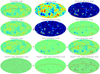 |
Fig. 1. First row: Gaussian CMB realisation (left), the filtered version (middle), and the square of the filtered map (right). The orange ellipse denotes the random dipole direction observed on large angular scales. For the squared map, dark blue corresponds to zero temperature, while for all other maps dark red and dark blue correspond to the largest negative and positive fluctuations in the map. Second row: product of the Gaussian map (left) and the squared filtered map (middle) generates the non-Gaussian contribution (right) that enhances the dipole in the power distribution. Third row: combination of the original Gaussian map (left) and the non-Gaussian term (middle) scaled by the factor βdimensionless = 1.77 × 10⁸ yielding a non-Gaussian map (right) with enhanced dipole modulation and a hot spot with excess kurtosis shown in the blue circle. Last row: as in the third row, but for scales ℓ = 100−200 only. The value of β is exaggerated here in order to make the effect visible by eye. |
We see by eye that this Gaussian realisation contains more large-scale fluctuations in the southern hemisphere than in the northern hemisphere (indicated by the orange oval). Such a random dipolar distribution of power is common to all Gaussian realisations. Since the direction of such a dipolar distribution is random, no evidence of this behaviour is seen when the mean is taken over many simulations. The large-scale fluctuations in the southern hemisphere are then enhanced, as shown in the second row of the figure. In the third row, the non-Gaussian term obtained in the second row is added to the Gaussian map, thereby enhancing the large-scale fluctuations in the southern hemisphere and giving rise to a dipolar modulation on large scales. We also note the non-Gaussian hot-spot created by the non-Gaussian term, as highlighted by the blue circle. For this specific realisation, the non-Gaussian feature is a hot spot since the largest fluctuation on the sky is positive. For realisations where the largest fluctuation is negative, a non-Gaussian cold spot will arise. However, since the hot spot is necessarily created on top of a hot fluctuation, a corresponding cold spot would be created on top of a cold fluctuation and the observed feature of a hot ring surrounding the cold spot (see anomaly A3 above) will not be created in this simplified model. Below (Eq. (3)) we describe a more sophisticated model that can reproduce all anomalies A1 to A6.
Finally, in the lowest row of Fig. 1, we present maps filtered to contain the angular scales for ℓ = 100−200 only, before and after adding the non-Gaussian term. The large-scale structure in the southern hemisphere in the Gaussian map has been imprinted on these smaller scales (as seen in the middle plot). Adding this small-scale structure tilts the random dipolar distribution of power on the sky for these scales towards the south, as in anomaly A2. This happens for all scales.
We thus propose an initial toy model, written as

to reproduce anomalies A1, A2, and A3. This model would leave a strong imprint of anomalies on all scales. In order to avoid anomaly A2 becoming too pronounced, and to obtain a map that is consistent with the observed CMB sky, the final term must itself be filtered. We therefore modify the above model as
![$$ \begin{aligned} T(\theta ,\phi ){\rm{ }} = {T_{\rm{G}}}(\theta ,\phi ) + \beta {\left[ {{T_{\rm{G}}}(\theta ,\phi )T_{\rm{F}}^2(\theta ,\phi )} \right]^{{\rm{Filtered}}}}, \end{aligned} $$](/articles/aa/full_html/2019/06/aa33698-18/aa33698-18-eq5.gif)
where
The filters wℓ and gℓ, and the amplitude β are then adjusted to test whether the anomalies can be reproduced. In addition to this model, we also tested a variant with similar behaviour,
![$$ \begin{aligned} T(\theta ,\phi )=T_\mathrm{G} (\theta ,\phi ) + \beta \left[T_\mathrm{G} (\theta ,\phi ) \left\{ T_\mathrm{G} ^2(\theta ,\phi )\right\} _F\right]^\mathrm{Filtered} \end{aligned} $$](/articles/aa/full_html/2019/06/aa33698-18/aa33698-18-eq8.gif)
The difference to the original model should be noted: the Gaussian field is squared before the filter wℓ is applied. In this paper results will always be based on the model specified by Eq. (3), unless we explicitly refer to the alternative Eq. (6).
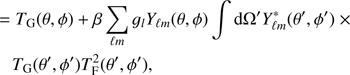
Figure 2 presents the filters wℓ and gℓ, shown as solid black lines, used for the majority of results in this paper. They correspond to one representative example of a huge variety of filters that, to different extents, can reproduce properties of the anomalies. Some other filters, commented on below, are also shown. The black filters are adjusted to the form shown in Fig. 2 in order to reproduce the shape of the power spectrum on large scales, specifically to reproduce anomalies A4 and A6, and to ensure that anomaly A2 is present on smaller scales.
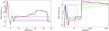 |
Fig. 2. Filter functions wℓ (left) and gℓ (right) used in our toy model. For gℓ, all filters except the blue filter have gℓ = −8 for ℓ = 2, which is not shown in order to make the filters more visible for all other multipoles. The black lines show the filters that form the basis for the majority of results presented in the paper. The coloured filters are equal to the black filter for multipoles where the coloured filters are not visible. Red line: a smoother version of the main filter; green line: similar to the black filter but slightly simpler with no change of sign in gℓ; blue dashed line: highly simplified wℓ; red dashed line: the alternative model which filters the squared Gaussian map; blue line: filter used for the model with Gaussian white noise maps. |
The shape defined for the black filters in Fig. 2 can be understood as follows. The oscillations in the lowest multipoles of wℓ give rise to the observed parity asymmetry, and were adjusted to reproduce the observed power spectrum oscillations for ℓ < 10. We did not attempt to reproduce the parity asymmetry at higher multipoles here, but given the strong correlations between wℓ and the shape of the power spectrum, a model with wiggles in this filter could give rise to odd-even features in the spectrum also at other multipoles in the same way as we have shown for ℓ < 10. The filter wℓ then rises incrementally to a plateau around ℓ = 21, after which it drops to zero at ℓ = 28. This allows the model to reproduce the large trough at ℓ ∼ 21. For ℓ > 27 the observed power spectrum no longer lies systematically below the model spectrum, thus wℓ can be zero for higher multipoles. We note that the purpose of the features of wℓ shown by the black line is to reproduce the particular features in the power spectrum. A completely flat wℓ filter which is zero for ℓ > 27 (as shown by the blue dashed line) can still give rise to all anomalies except parity asymmetry (A6) and quadrupole-octopole alignment (A5) for which a higher value of wℓ at ℓ = 2 and ℓ = 3 is necessary.
The black filter gℓ in Fig. 2 is negative up to ℓ = 27 where it suddenly becomes positive and then gradually decreases towards zero at high ℓ. For large scales, gℓ is negative in order to subtract power for ℓ < 27 making the power spectrum low for this multipole range, a positive gℓ here instead would yield a large-scale power spectrum with high amplitude. Then, in order to reproduce anomaly A2 on small scales, gℓ needs to be non-zero up to ℓ ∼ 1500 (but can be positive, negative, or oscillate between the two). The filter gℓ needs to decrease slowly to zero towards ℓ ∼ 1500 in order to limit A2. The strong negative value for ℓ = 2 in gℓ is in order to ensure a small quadrupole, but will also strongly influence the original quadrupole generating correlations with the octopole as in anomaly A5.
The black filters in Fig. 2 are constructed from a combination of step functions in order to obtain the general properties described above. A physical model would more naturally have a smoother scale dependence, but the purpose of this paper is to describe a toy model that presents the general features of scale dependences that can give rise to the CMB anomalies. We do not attempt to derive a model that can be fitted to the data here, since the number of degrees of freedom is too large, and a theoretical model would be needed that naturally gives rise to this scale dependence for a minimum number of additional parameters. Such models will be explored in future work (Bartolo et al., in prep.).
Figure 2 presents some additional representative examples of filters that can reproduce most or all of the anomalies. The red lines show a smoother version of the black filter giving very similar results. The filter shown in green differs from the black filter in that it is negative for all multipoles, again reproducing all anomalies. The blue dashed filter is much simpler; since wℓ is flat, the odd-even oscillations in the power spectrum for low multipoles are not reproduced (thus anomaly A6 disappears) and the trough at ℓ = 21 is not visible. Even with this simple filter, several anomalies are present. The red dashed lines represent the filters that are used for the alternative model in Eq. (6). The blue filter is used for Gaussian maps replaced by white noise maps as described below. Due to limitations in available CPU hours, only the maps based on the black filters were studied in detail using 3000 simulations, with 1000 maps simulated for the other filters.
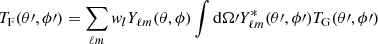
In Fig. 3 we show the non-Gaussian term for a simulated map generated using the black filters in Fig. 2. The figure shows one of the maps from our simulation pipeline described below where a dimensionless1 amplitude βdimensionless = 4.4 × 10⁶ is used. For this realisation, the northern hemisphere of the Gaussian map has more large-scale power, which is then enhanced in the non-Gaussian map. The negative (or possibly oscillating) gℓ for larger scales makes the non-Gaussian term more complicated and less intuitive than the simplified illustration in Fig. 1. In this case, fluctuations on some scales are enhanced and others are suppressed. In particular, strong cold fluctuations can now appear superposed on larger hot fluctuations and vice versa. In this way, a cold spot can be found with a hot surrounding ring as observed in the Planck data (see anomaly A3 above). This is clearly seen in Fig. 4 which shows a zoomed-in image of the cold spot from the simulated map in the lower panel of Fig. 3.
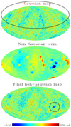 |
Fig. 3. Top: original simulated Gaussian map. The circle indicates the hemisphere with the most large-scale power. Middle: additional term used in our non-Gaussian model scaled by βdimensionless = 4.4 × 10⁶, as used for the simulated model. Bottom: non-Gaussian map created by the addition of the second map to the Gaussian map. The circle highlights a cold spot surrounded by a hot ring. |
Comparing the toy model in Eq. (3) to the theoretical gNL-model in Eq. (1), some similarities are apparent, but clearly a scale-dependent gNL model is required where the scale dependence defines the shape of the filters wℓ and gℓ. Unlike physical gNL models, we note that a full CMB map with radiative transfer is included in all three fields in the non-Gaussian term in Eq. (3). As is discussed later, the spectrum used for the Gaussian map is actually unimportant. The anomalies can be adequately reproduced using either a pure Sachs-Wolfe or a white noise spectrum to generate the Gaussian map used as an input for creating the non-Gaussian term.
The term  has a dipole (ℓ = 1) component by construction, even if TF(θ, ϕ) has a zero dipole. This directly induces a modulation in the final map, as in Eq. (2), which is much larger than observed in the data. A physical model must therefore have an additional filter that effectively reduces this dipolar term (or, by coincidence, this dipole is small in the actual Universe). In the test simulations used here, this dipole is set to zero by hand, except for the alternative model given by Eq. (6) where it is resolved if wℓ is low or zero for ℓ = 1. We further note that in order for the final map to have a small-scale power spectrum that matches the data, the total amplitude of the original map must be adjusted slightly. This corresponds to a cosmological model with a slightly lower amplitude of primordial fluctuations.
3. Simulations and comparison with data
In order to compare the probability of finding the observed anomalies in toy model simulations to that in Gaussian simulations, we used a set of 3000 simulated Gaussian Planck maps (Planck Collaboration XII 2016) which were propagated through the SMICA foreground cleaning pipeline in order to compare them with the data cleaned with SMICA foreground subtraction method (Planck Collaboration IX 2016). The simulations were divided into three sets of 1000 simulations. Set 1 was used to calibrate the probabilities used to find p-values for the anomalies, set 2 was used to create the non-Gaussian simulations, and set 3 was used to compare Gaussian with non-Gaussian simulations.
We use anomaly A1 as an example of how these three sets were used:
-
1.
The dipole modulation amplitudes (corresponding to β in Eq. (2) with a dipole as the modulation field) were estimated for all three sets of simulations for a given maximum multipole ℓmax.
-
2.
The dipole modulation amplitude of one selected simulation in set 3 (Gaussian) was compared to all 1000 Gaussian simulations in set 1 in order to find the fraction of maps in set 1 with a larger amplitude than the selected simulation from set 3. This fraction is the p-value for this given set 3 simulation.
-
3.
This procedure was repeated for all 1000 simulations in set 3 to determine 1000 p-values for a given ℓmax.
-
4.
Points 2 and 3 were repeated using set 2 in place of set 3: in this way we compared the dipole modulation amplitudes of all 1000 non-Gaussian simulations in set 2 to set 1.
In Fig. 5 we show the mean power spectrum of these simulated maps compared to the Planck best fit theoretical ΛCDM model (Planck Collaboration XIII 2016) and the estimated Planck power spectrum. We clearly see, as expected from the construction of the filters, that the new model is in better agreement with the data for low multipoles. In particular the low power spectrum (anomaly A4) and the even-odd asymmetry (anomaly A6) are evident for some multipoles. For ℓ > 50 the mean of the simulated spectra and the best fit model are almost identical and are not shown.
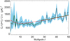 |
Fig. 5. Angular power spectrum: estimated Cℓ from Planck data (black; Planck Collaboration XI 2016); mean Cℓ of 1000 non-Gaussian simulations (green); and Cℓ of the theoretical best fit ΛCDM model of Planck Collaboration XIII (2016; red). The shaded area presents 2σ error bars from Planck Collaboration XI (2016). |
In Fig. 6, we show the probability of the dipole modulation amplitude in a given map as a function of multipole. In order to make the analysis of dipolar modulation computationally feasible, the simulations for this anomaly were analysed without using a mask. However, since the first set of 1000 simulations used to calibrate the p-values is treated in the same way, we do not expect the results to be biased. We note that the calculations were performed following the description in Planck Collaboration XVI (2016), but without the mask. For all other analyses in this paper, we performed the analysis for the data and simulations with the same pipeline and, as shown in the figure, obtain results consistent with previous papers.
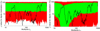 |
Fig. 6. p-values for dipolar modulation, to be compared with Fig. 30 in Planck Collaboration XVI (2016). Green and red bands show the 1σ and 2σ spread of p-values measured in 1000 Gaussian simulations (left plot) and 1000 non-Gaussian model simulations (right plot). In both plots, the black line shows the p-values for Planck data taken from Fig. 30 in Planck Collaboration XVI (2016). These p-values show the percentage of Gaussian simulations having larger dipolar modulation up to the given multipole than the Planck data (calibrated with 1000 Gaussian simulations). |
Figure 6 corresponds to Fig. 30 in Planck Collaboration XVI (2016). The green and red areas show the 68% and 95% intervals from Gaussian simulations (left panel) and our toy model simulations (right panel). The black line corresponds to the Planck result from Planck Collaboration XVI (2016). The left panel shows that the p-values for the data are outside the 68% interval for almost all multipoles ℓ < 200 compared to Gaussian simulations. In addition there are several dips outside the 95% interval. Conversely, the Planck data points seem consistent with our toy model, as shown in the right panel. The clear dip of the 68% green range for ℓ < 100 indicates that a strong dipolar modulation is expected on large angular scales in this model.
In Fig. 7 we show the probability of alignment of the power distribution dipoles up to a certain multipole (compare Fig. 36 in Planck Collaboration XVI 2016). The green and red areas show the 68% and 95% intervals from Gaussian simulations (left panel) and our toy model simulations (right panel). The black line shows the results determined from the Planck data and has been taken from Fig. 36 in Planck Collaboration XVI (2016). In the left panel, it can be seen that the data, as compared to Gaussian simulations, always lie outside the 95% interval for ℓ > 200. The right panel demonstrates that the behaviour of the data is consistent with the non-Gaussian toy model.
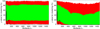 |
Fig. 7. p-values for alignment of the spatial power distribution dipoles up to a given multipole. This is the equivalent plot to Fig. 36 in Planck Collaboration XVI (2016). The green and red bands indicate the 1σ and 2σ spread of p-values measured in 1000 Gaussian simulat ions (left panel) and 1000 non-Gaussian model simulations (right panel). The black line corresponds to the p-values for Planck data taken from Fig. 36 in Planck Collaboration XVI (2016). These p-values show the percentage of Gaussian simulations with a larger alignment of the spatial power distribution up to the given multipole (calibrated with 1000 Gaussian simulations). |
Figure 8 shows the kurtosis for wavelet coefficients using spherical Mexican Hat wavelets and the same wavelet scales as in Vielva et al. (2004). The left panel shows the kurtosis compared to Gaussian simulations (green and red shaded bands). For scales 7–9 the Planck data show excess kurtosis outside the 95% confidence region. In the toy model (right panel), we see a clearly enhanced probability for an excess kurtosis at exactly these scales. The data points for scales 7–9 are now within the 68% confidence region. The scale-dependent kurtosis of wavelet coefficients also put limits on a possible scale-dependence of a gNL non-Gaussianity. The plot shows that our model predicts a level of kurtosis consistent with current observational constraints.
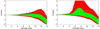 |
Fig. 8. Kurtosis of wavelet coefficients for the wavelet scales defined in Vielva et al. (2004). Green and red bands show the 1σ and 2σ spread of kurtosis values in 1000 Gaussian simulations (left panel) and 1000 non-Gaussian model simulations (right panel). The black crosses indicate the kurtosis values computed from the Planck data; the grey crosses show the values derived after masking the brightest spot for the given wavelet scale. The grey lines show the 2σ limits after masking the brightest spot for the given scale. The masking is performed with a disc of radius 5 degrees. |
Vielva et al. (2004) have shown that the excess observed kurtosis disappears after masking the highest temperature outlier in the map. This is shown in Fig. 8 where the grey crosses represent the kurtosis values computed from the data after masking, and the grey lines indicate the 2σ confidence interval after masking the simulations. For the toy models, there is a clear drop in kurtosis after masking the brightest spot showing that the excess kurtosis in the toy model simulations is indeed mainly associated with one strong hot or cold spot, as for the observational data.
Figure 9 shows how the angular separation between the quadrupole and octopole preferred directions are distributed in Gaussian simulations (left panel) and toy model simulations (right panel). The vertical black line represents this angle for the Planck data. The left panel indicates that the probability falls for smaller angles. For toy model simulations, the distribution is somewhat flatter, therefore the quadrupole-octopole alignment seen in the data can be considered less anomalous.
 |
Fig. 9. Angular separation between the quadrupole and octopole preferred directions. Left panel: distribution of this angular distance for 1000 Gaussian simulations, right panel: corresponding distribution for 1000 non-Gaussian simulations. The vertical black line represents the angular distance observed in the Planck data. |
Finally, the direction of dipolar modulation, the cold spot and the directions of the alignment asymmetry all seem to be converging. In particular, the angular distance between the direction of dipolar modulation and the cold spot is 32° in the Planck data. In Fig. 10 we show the distribution of angular distances between the dipolar modulation and the cold/hot spot in Gaussian simulations (left panel) or toy model simulations (right panel). The position of the cold/hot spot is clearly strongly correlated with the dipolar modulation direction in the toy model simulations and in excellent agreement with the data. A similar correlation of direction with the small-scale hemispherical asymmetry is seen in toy model simulations with a strong alignment asymmetry.
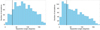 |
Fig. 10. Angular distance between hot or cold spot and direction of max dipolar modulation. The distribution of the angular distance is shown for 1000 Gaussian simulations (left panel) and 1000 non-Gaussian simulations (rights panel). The vertical black line corresponds to the angular distance for the Planck data. |
4. Discussion and conclusions
In this paper we have shown that the CMB anomalies, including apparent deviations from statistical isotropy and features in the power spectrum can arise from non-Gaussianity. In particular, in the analyses of simulated toy model maps using a gNL-like non-Gaussian term of the form given in Eq. (3) or (6), all of the most commonly discussed anomalies are reproduced. To what extent the different anomalies are present depends on the filters wℓ and gℓ (which would correspond to specific scale dependences of the primordial non-Gaussianity trispectrum gNL). Even very simple forms of these filters give rise to several anomalies in our phenomenological model, but a physical model would be required to predict their shape with a minimum number of free parameters.
Figure 5 demonstrates how such a toy model results in low power on large angular scales, including the quadrupole, and parity asymmetry for the first few multipoles. Then, in Figs. 6–9, we see evidence that various features of the data, characterised as 2–3σ outliers when compared to Gaussian simulations, are more consistent with the expectations of these toy model simulations.
It should be noted that the filter functions selected here, which effectively define scale dependence, are simple. Further work is needed to assess whether these functions are realistic in the context of a primordial underlying model or otherwise. However, it may be that a physical model could give rise to more complex filters and still reproduce the anomalies if it essentially mimics the main features displayed by the phenomenological model focused on in this work.
We have focused on gNL models here. While fNL and τNL models may reproduce some of the anomalies, they cannot easily reproduce all of them, whereas gNL models appear to. Anomaly A1 and possibly A2 could arise in τNL models (Adhikari et al. 2018), but these models would not generally give a non-Gaussian hot or cold spot. For this an enhancement of the original Gaussian fluctuations would be necessary, which is not easily achieved in a τNL model where the non-Gaussian term is strongly influenced by an independent field. For the same reason, they also would not easily give quadrupole-octopole alignment, where the non-Gaussian term also needs to be strongly correlated with the Gaussian term.
Similarly, it would be difficult for an fNL model to give large-scale power deficit and quadrupole-octopole alignment, since for a second-order term positive fluctuations would be enhanced, while negative fluctuations would be erased. An excess kurtosis would also not arise from a second-order term (at lowest order in the perturbations). As we have seen in this paper, the reason why gNL models can generate all of the anomalies originates from the way in which the non-Gaussian term correlates to the Gaussian term.
In our toy model (Eq. (3)), we have used CMB maps that include the effects of radiative transfer as the basis of the non-Gaussian term. Inspection of Eq. (1) indicates that, for an inflationary model, it is the non-Gaussian third-order term in the gravitational potential (with an overall amplitude gNL) that would be transferred to the CMB anisotropies via the CMB radiation transfer function. In order to be more consistent with this scenario, we generated Gaussian maps with (1) a pure Sachs-Wolfe spectrum and (2) a pure white noise spectrum (Cℓ = const). We then generated the non-Gaussian term based on these Gaussian maps, and then applied radiative transfer by changing the variance of the aℓm coefficients of the final maps in order to obtain a spectrum consistent with Planck best fit. In both cases, after modifying gℓ and wℓ accordingly, all anomalies are again reproduced.
It should be noted that we set the filter wℓ to zero for ℓ > 27 in order to minimise the impact on the power spectrum for larger multipoles. The Planck data indicates that the power spectrum is low up to ℓ = 27. Nevertheless, we tested the effect of (i) setting wℓ to zero for ℓ > 15 and (ii) setting wℓ to zero for ℓ > 50 with a non-zero filter extending to ℓ = 50. In both cases the spectrum was modified to be low in the range where wℓ is non-zero, thereby reducing the consistency with the Planck power spectrum. Furthermore, the scales of the cold or hot spot and the dipolar modulation were both altered, in general resulting in worse agreement with the data. We interpret this as an indication of correlation between the angular scales where the power spectrum is low and the angular scales of dipolar modulation (A1) and the cold spot (A3). A similar correlation is seen in that the filters that cause quadrupole-octopole alignment (A5) also give a low quadrupole. We note, however, that there is considerable freedom in the way that the filters can be adjusted; therefore, we restricted our investigations to simple extensions of the toy model used here.
In Figs. 6–9, we show how the anomalies are easily reproduced by the toy model simulations. However, in general, not all anomalies will be present in a given simulation; there is considerable variation in terms of which anomalies are seen from realisation to realisation, and some simulations do not show clear signs of any anomalous behaviour. Furthermore, as shown in Fig. 3, the non-Gaussianity, and thereby the anomalies, may only be visible in localised parts of the sky that are either partially or fully rejected from further analysis by the application of a suitable Galactic mask. These issues make it difficult to predict what we should expect for polarisation data in our toy model. If we assume that the non-Gaussian polarisation term can be obtained through a similar mechanism, then–given that the signal is only partially correlated with the temperature realisation–we would not necessarily expect the same anomalies to appear, either with the same amplitude or a similar direction. Indeed, without a theoretical model, we cannot make clear predictions for what to expect in polarisation.
Finally, we reiterate that the scope of this paper was to guide theoretical research by proposing a general form for a non-Gaussian term that might be the origin of all of the observed CMB anomalies. The next step must then be to determine whether an inflationary model exists that can reproduce the main features of the phenomenological model proposed in this paper. An actual physical model could take a slightly different form with different filters and still reproduce the anomalies. Then, only when a physically motivated model is found can a complete comparison to data be undertaken, and predictions made for other anomalies and possible features in the CMB polarisation signal. This should help to alleviate the “multiplicity of tests” arguments (Dvorkin et al. 2008; Contreras et al. 2017) made against claims of anomalies in the data.
Dimensionless β refers to the amplitude determined when the maps are made dimensionless after dividing by 2.73 K in Eq. (3).
Acknowledgments
The results in this paper are based on observations obtained with Planck (http://www.esa.int/Planck), an ESA science mission with instruments and contributions directly funded by ESA Member States, NASA, and Canada. The simulations were performed on resources provided by UNINETT Sigma2 – the National Infrastructure for High Performance Computing and Data Storage in Norway. NB and ML acknowledge partial financial support by ASI Grant No. 2016-24-H.0. Maps and results have been derived using the Healpix software package developed by Górski et al. (2005).
References
- Adhikari, S., Shandera, S., & Erickeck, A. L. 2016, Phys. Rev. D, 93, 023524 [NASA ADS] [CrossRef] [Google Scholar]
- Adhikari, S., Deutsch, A.-S., & Shandera, S. 2018, Phys. Rev. D, 98, 023520 [NASA ADS] [CrossRef] [Google Scholar]
- Agullo, I. 2015, Phys. Rev. D, 92, 064038 [NASA ADS] [CrossRef] [Google Scholar]
- Akrami, Y., Fantaye, Y., Eriksen, H. K., et al. 2014, ApJ, 784, L42 [NASA ADS] [CrossRef] [Google Scholar]
- Ashoorioon, A., & Koivisto, T. 2016, Phys. Rev. D., 94, 043009 [NASA ADS] [CrossRef] [Google Scholar]
- Assadullahi, H., Firouzjahi, H., Namjoo, M. H., & Wands, D. 2015, JCAP, 1504, 017 [NASA ADS] [CrossRef] [Google Scholar]
- Axelsson, M., Fantaye, Y., Hansen, F. K., et al. 2013, ApJ, 773, L3 [NASA ADS] [CrossRef] [Google Scholar]
- Banday, A. J., Zaroubi, S., & Górski, K. M. 2000, ApJ, 533, 575 [NASA ADS] [CrossRef] [Google Scholar]
- Bennett, C. L., Halpern, M., Hinshaw, G., et al. 2003, ApJS, 148, 1 [NASA ADS] [CrossRef] [Google Scholar]
- Byrnes, C. T., & Tarrant, E. R. M. 2015, JCAP, 1602, 029 [Google Scholar]
- Byrnes, C. T., Sasaki, M., & Wands, D. 2006, Phys. Rev. D, 74, 123519 [NASA ADS] [CrossRef] [Google Scholar]
- Byrnes, C. T., Regan, D., Seery, D., & Tarrant, E. R. M. 2016, JCAP, 1606, 025 [NASA ADS] [CrossRef] [Google Scholar]
- Contaldi, C. R., Peloso, M., Kofman, K., & Linde, A. 2003, JCAP, 0307, 002 [Google Scholar]
- Contreras, D., Zibin, J. P., Scott, D., Banday, A. J., & Górski, K. M. 2017, Phys. Rev. D, 96, 123522 [NASA ADS] [CrossRef] [Google Scholar]
- Contreras, D., Hutchinson, J., Moss, A., Scott, D., & Zibin, J. P. 2018, Phys. Rev. D, 97, 063504 [NASA ADS] [CrossRef] [Google Scholar]
- Dai, L., Jeong, D., Kamionkowski, M., & Chluba, J. 2013, Phys. Rev. D, 87, 123005 [NASA ADS] [CrossRef] [Google Scholar]
- D’Amico, G., Gobbetti, R., Kleban, M., & Schillo, M. 2013, JCAP, 1311, 013 [NASA ADS] [CrossRef] [Google Scholar]
- Dvorkin, C., Peiris, H. V., & Hu, W. 2008, Phys. Rev. D, 77, 063008 [NASA ADS] [CrossRef] [Google Scholar]
- Eriksen, H. K., Hansen, F. K., Banday, A. J., Górski, K. M., & Lilje, P. B. 2004, ApJ, 605, 14 [NASA ADS] [CrossRef] [Google Scholar]
- Eriksen, H. K., Banday, A. J., Górski, K. M., Hansen, F. K., & Lilje, P. B. 2007, ApJ, 660, L81 [NASA ADS] [CrossRef] [Google Scholar]
- Erickcek, A. L., Kamionkowski, M., & Carroll, S. M. 2008, Phys. Rev. D, 78, 123520 [NASA ADS] [CrossRef] [Google Scholar]
- Erickcek, A. L., Hirata, C. M., & Kamionkowski, M. 2009, Phys. Rev. D, 80, 083507 [NASA ADS] [CrossRef] [Google Scholar]
- Ferreira, P. G., Magueijo, J., & Górski, K. M. 1998, ApJ, 503, L1 [NASA ADS] [CrossRef] [Google Scholar]
- Firouzjahi, H., Gong, J.-O., & Namjoo, M. H. 2014, JCAP, 1411, 037 [NASA ADS] [CrossRef] [Google Scholar]
- Gangui, A., Lucchin, F., Matarrese, S., & Mollerach, S. 1994, ApJ, 430, 447 [NASA ADS] [CrossRef] [Google Scholar]
- Gordon, C., Hu, W., Huterer, D., & Crawford, T. 2005, Phys. Rev. D, 72, 103002 [NASA ADS] [CrossRef] [Google Scholar]
- Górski, K. M., Hivon, E., Banday, A. J., et al. 2005, ApJ, 699, 759 [CrossRef] [Google Scholar]
- Gruppuso, A., Kitazawa, N., Mandolesi, N., Natoli, P., & Sagnotti, A. 2016, Phys. Dark Univ., 11, 68 [CrossRef] [Google Scholar]
- Gruppuso, A., Kitazawa, N., Lattanzi, M., et al. 2018, PDU, 20, 49 [NASA ADS] [Google Scholar]
- Hansen, F. K., Górski, K. M., & Hivon, E. 2004, ApJ, 354, 641 [Google Scholar]
- Hansen, F. K., Banday, A. J., Górski, K. M., Eriksen, H. K., & Lilje, P. B. 2009, ApJ, 704, 1448 [NASA ADS] [CrossRef] [Google Scholar]
- Hoftuft, J., Eriksen, H. K., Banday, A. J., et al. 2009, ApJ, 699, 985 [NASA ADS] [CrossRef] [Google Scholar]
- Jazayeri, S., Akrami, Y., Firouzjahi, H., Solomon, A. R., & Wang, Y. 2014, JCAP, 1411, 044 [NASA ADS] [CrossRef] [Google Scholar]
- Kanno, S., Sasaki, M., & Tanaka, T. 2013, PTEP, 2013, 111E01 [Google Scholar]
- Kenton, Z., Mulryne, D. J., & Thomas, S. 2015, Phys. Rev. D, 92, 023505 [NASA ADS] [CrossRef] [Google Scholar]
- Kobayashi, T., Cortes, M., & Liddle, A. R. 2015, JCAP, 1505, 029 [NASA ADS] [CrossRef] [Google Scholar]
- Kohri, K., Lin, C.-M., & Matsuda, T. 2014, JCAP, 1408, 026 [NASA ADS] [CrossRef] [Google Scholar]
- Komatsu, E., & Spergel, D. N. 2001, Phys. Rev. D, 63, 063002 [NASA ADS] [CrossRef] [Google Scholar]
- Komatsu, E., Wandelt, B. D., Spergel, D. N., Banday, A. J., & Górski, K. M. 2002, ApJ, 566, 19 [NASA ADS] [CrossRef] [Google Scholar]
- Liddle, A. R., & Cortês, M. 2013, Phys. Rev. Lett., 111, 111302 [NASA ADS] [CrossRef] [Google Scholar]
- Liu, Z.-G., Guo, Z.-K., & Piao, Y.-S. 2013, Phys. Rev. D, 88, 063539 [NASA ADS] [CrossRef] [Google Scholar]
- Lyth, D. H. 2013, JCAP, 1308, 007 [NASA ADS] [CrossRef] [Google Scholar]
- Lyth, D. H. 2015, JCAP, 1504, 039 [NASA ADS] [CrossRef] [Google Scholar]
- Mazumdar, A., & Wang, L. 2013, JCAP, 1310, 049 [NASA ADS] [CrossRef] [Google Scholar]
- McDonald, J. 2013a, JCAP, 1307, 043 [NASA ADS] [CrossRef] [Google Scholar]
- McDonald, J. 2013b, JCAP, 1311, 041 [NASA ADS] [CrossRef] [Google Scholar]
- McDonald, J. 2014, Phys. Rev. D, 89, 127303 [NASA ADS] [CrossRef] [Google Scholar]
- Muir, J., Adhikari, S., & Huterer, D. 2018, Phys. Rev. D, 98, 023521 [NASA ADS] [CrossRef] [Google Scholar]
- Namjoo, M. H. 2014, Phys. Rev. D, 89, 063511 [NASA ADS] [CrossRef] [Google Scholar]
- Namjoo, M. H., Baghram, S., & Firouzjahi, F. 2013, Phys. Rev. D, 88, 083527 [NASA ADS] [CrossRef] [Google Scholar]
- Namjoo, M. H., Abolhasani, A. A., Baghram, S., & Firouzjahi, H. 2014, JCAP, 1408, 002 [NASA ADS] [CrossRef] [Google Scholar]
- Okamoto, T., & Hu, W. 2002, Phys. Rev. D, 66, 063008 [NASA ADS] [CrossRef] [Google Scholar]
- Pando, J., Valls-Gabaud, D., & Fang, L. 1998, PRL, 81, 4561 [NASA ADS] [CrossRef] [Google Scholar]
- Planck Collaboration XXIII. 2014, A&A, 571, A23 [NASA ADS] [CrossRef] [EDP Sciences] [MathSciNet] [PubMed] [Google Scholar]
- Planck Collaboration XXIV. 2014, A&A, 571, A24 [NASA ADS] [CrossRef] [EDP Sciences] [Google Scholar]
- Planck Collaboration IX. 2016, A&A, 594, A9 [NASA ADS] [CrossRef] [EDP Sciences] [Google Scholar]
- Planck Collaboration XI. 2016, A&A, 594, A11 [NASA ADS] [CrossRef] [EDP Sciences] [Google Scholar]
- Planck Collaboration XII. 2016, A&A, 594, A12 [NASA ADS] [CrossRef] [EDP Sciences] [Google Scholar]
- Planck Collaboration XIII. 2016, A&A, 594, A13 [NASA ADS] [CrossRef] [EDP Sciences] [Google Scholar]
- Planck Collaboration XVI. 2016, A&A, 594, A16 [NASA ADS] [CrossRef] [EDP Sciences] [Google Scholar]
- Planck Collaboration XVII. 2016, A&A, 594, A17 [NASA ADS] [CrossRef] [EDP Sciences] [Google Scholar]
- Planck Collaboration XX. 2016, A&A, 594, A20 [NASA ADS] [CrossRef] [EDP Sciences] [Google Scholar]
- Schmidt, F., & Huai, L. 2013, Phys. Rev. Lett., 110, 011301 [NASA ADS] [CrossRef] [PubMed] [Google Scholar]
- Tegmark, M., de Oliveira-Costa, A., & Hamilton, A. J. 2003, Phys. Rev. D, 68, 123523 [NASA ADS] [CrossRef] [Google Scholar]
- Verde, L., Wang, L., Heavens, A. F., & Kamionkowski, M. 2000, MNRAS, 313, 141 [NASA ADS] [CrossRef] [Google Scholar]
- Vielva, P., Martinez-Gonzalez, E., Barreiro, R. B., Sanz, J. L., & Cayon, L. 2004, ApJ, 609, 22 [NASA ADS] [CrossRef] [Google Scholar]
- Wang, L., & Kamionkowski, M. 2000, Phys. Rev. D, 61, 063504 [NASA ADS] [CrossRef] [Google Scholar]
- Wang, L., & Mazumdar, A. 2013, Phys. Rev. D, 88, 023512 [NASA ADS] [CrossRef] [Google Scholar]
- Zarei, M. 2015, Eur. Phys. J. C, 75, 268 [NASA ADS] [CrossRef] [EDP Sciences] [Google Scholar]
- Zhu, T., Wang, A., Kirsten, K., Cleaver, G., & Sheng, Q. 2018, Phys. Rev. D, 97, 043501 [NASA ADS] [CrossRef] [Google Scholar]
All Figures
|
Fig. 1. First row: Gaussian CMB realisation (left), the filtered version (middle), and the square of the filtered map (right). The orange ellipse denotes the random dipole direction observed on large angular scales. For the squared map, dark blue corresponds to zero temperature, while for all other maps dark red and dark blue correspond to the largest negative and positive fluctuations in the map. Second row: product of the Gaussian map (left) and the squared filtered map (middle) generates the non-Gaussian contribution (right) that enhances the dipole in the power distribution. Third row: combination of the original Gaussian map (left) and the non-Gaussian term (middle) scaled by the factor βdimensionless = 1.77 × 10⁸ yielding a non-Gaussian map (right) with enhanced dipole modulation and a hot spot with excess kurtosis shown in the blue circle. Last row: as in the third row, but for scales ℓ = 100−200 only. The value of β is exaggerated here in order to make the effect visible by eye. |
| In the text | |
|
Fig. 2. Filter functions wℓ (left) and gℓ (right) used in our toy model. For gℓ, all filters except the blue filter have gℓ = −8 for ℓ = 2, which is not shown in order to make the filters more visible for all other multipoles. The black lines show the filters that form the basis for the majority of results presented in the paper. The coloured filters are equal to the black filter for multipoles where the coloured filters are not visible. Red line: a smoother version of the main filter; green line: similar to the black filter but slightly simpler with no change of sign in gℓ; blue dashed line: highly simplified wℓ; red dashed line: the alternative model which filters the squared Gaussian map; blue line: filter used for the model with Gaussian white noise maps. |
| In the text | |
|
Fig. 3. Top: original simulated Gaussian map. The circle indicates the hemisphere with the most large-scale power. Middle: additional term used in our non-Gaussian model scaled by βdimensionless = 4.4 × 10⁶, as used for the simulated model. Bottom: non-Gaussian map created by the addition of the second map to the Gaussian map. The circle highlights a cold spot surrounded by a hot ring. |
| In the text | |
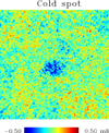 |
Fig. 4. Cold spot with the hot ring from the simulation shown in Fig. 3. |
| In the text | |
|
Fig. 5. Angular power spectrum: estimated Cℓ from Planck data (black; Planck Collaboration XI 2016); mean Cℓ of 1000 non-Gaussian simulations (green); and Cℓ of the theoretical best fit ΛCDM model of Planck Collaboration XIII (2016; red). The shaded area presents 2σ error bars from Planck Collaboration XI (2016). |
| In the text | |
|
Fig. 6. p-values for dipolar modulation, to be compared with Fig. 30 in Planck Collaboration XVI (2016). Green and red bands show the 1σ and 2σ spread of p-values measured in 1000 Gaussian simulations (left plot) and 1000 non-Gaussian model simulations (right plot). In both plots, the black line shows the p-values for Planck data taken from Fig. 30 in Planck Collaboration XVI (2016). These p-values show the percentage of Gaussian simulations having larger dipolar modulation up to the given multipole than the Planck data (calibrated with 1000 Gaussian simulations). |
| In the text | |
|
Fig. 7. p-values for alignment of the spatial power distribution dipoles up to a given multipole. This is the equivalent plot to Fig. 36 in Planck Collaboration XVI (2016). The green and red bands indicate the 1σ and 2σ spread of p-values measured in 1000 Gaussian simulat ions (left panel) and 1000 non-Gaussian model simulations (right panel). The black line corresponds to the p-values for Planck data taken from Fig. 36 in Planck Collaboration XVI (2016). These p-values show the percentage of Gaussian simulations with a larger alignment of the spatial power distribution up to the given multipole (calibrated with 1000 Gaussian simulations). |
| In the text | |
|
Fig. 8. Kurtosis of wavelet coefficients for the wavelet scales defined in Vielva et al. (2004). Green and red bands show the 1σ and 2σ spread of kurtosis values in 1000 Gaussian simulations (left panel) and 1000 non-Gaussian model simulations (right panel). The black crosses indicate the kurtosis values computed from the Planck data; the grey crosses show the values derived after masking the brightest spot for the given wavelet scale. The grey lines show the 2σ limits after masking the brightest spot for the given scale. The masking is performed with a disc of radius 5 degrees. |
| In the text | |
|
Fig. 9. Angular separation between the quadrupole and octopole preferred directions. Left panel: distribution of this angular distance for 1000 Gaussian simulations, right panel: corresponding distribution for 1000 non-Gaussian simulations. The vertical black line represents the angular distance observed in the Planck data. |
| In the text | |
|
Fig. 10. Angular distance between hot or cold spot and direction of max dipolar modulation. The distribution of the angular distance is shown for 1000 Gaussian simulations (left panel) and 1000 non-Gaussian simulations (rights panel). The vertical black line corresponds to the angular distance for the Planck data. |
| In the text | |
Current usage metrics show cumulative count of Article Views (full-text article views including HTML views, PDF and ePub downloads, according to the available data) and Abstracts Views on Vision4Press platform.
Data correspond to usage on the plateform after 2015. The current usage metrics is available 48-96 hours after online publication and is updated daily on week days.
Initial download of the metrics may take a while.