| Issue |
A&A
Volume 624, April 2019
|
|
|---|---|---|
| Article Number | A141 | |
| Number of page(s) | 24 | |
| Section | Catalogs and data | |
| DOI | https://doi.org/10.1051/0004-6361/201834656 | |
| Published online | 26 April 2019 | |
The MUSE-Wide Survey: survey description and first data release⋆,⋆⋆
1
Leibniz-Institut für Astrophysik, Potsdam (AIP), An der Sternwarte 16, 14482 Potsdam, Germany
e-mail: This email address is being protected from spambots. You need JavaScript enabled to view it.
2
Department of Astronomy, Stockholm University, AlbaNova University Centre, 106 91 Stockholm, Sweden
3
Institute of Astronomy, University of Cambridge, Madingley Road, Canbridge CB3 0HA, UK
4
Department of Physics, University of Malta, Msida MSD 2080, Malta
5
Institute of Space Sciences & Astronomy, University of Malta, Msida MSD 2080, Malta
6
Univ. Lyon, ENS de Lyon, CNRS, Centre de Recherche Astrophysique de Lyon UMR5574, 69230 Saint-Genis-Laval, France
7
Leiden Observatory, Leiden University, PO Box 9513, 2300 RA Leiden, The Netherlands
8
Instituto de Astrofíica e Ciências do Espaço, Universidade do Porto, CAUP, Rua das Estrelas, 4150-762 Porto, Portugal
Received:
15
November
2018
Accepted:
20
February
2019
Abstract
We present the MUSE-Wide survey, a blind, 3D spectroscopic survey in the CANDELS/GOODS-S and CANDELS/COSMOS regions. The final survey will cover 100 × 1 arcmin2 MUSE fields. Each MUSE-Wide pointing has a depth of one hour and hence targets more extreme and more luminous objects over ten times the area of the MUSE-Deep fields. The legacy value of MUSE-Wide lies in providing “spectroscopy of everything” without photometric pre-selection. We describe the data reduction, post-processing and PSF characterization of the first 44 CANDELS/GOODS-S MUSE-Wide pointings released with this publication. Using a 3D matched filtering approach we detect 1602 emission line sources, including 479 Lyman-α (Lyα) emitting galaxies with redshifts 2.9 ≲ z ≲ 6.3. We cross-matched the emission line sources to existing photometric catalogs, finding almost complete agreement in redshifts (photometric and spectroscopic) and stellar masses for our low redshift (z < 1.5) emitters. At high redshift, we only find ∼55% matches to photometric catalogs. We encounter a higher outlier rate and a systematic offset of Δz ≃ 0.2 when comparing our MUSE redshifts with photometric redshifts from the literature. Cross-matching the emission line sources with X-ray catalogs from the Chandra Deep Field South, we find 127 matches, mostly in agreement with the literature redshifts, including ten objects with no prior spectroscopic identification. Stacking X-ray images centered on our Lyα emitters yields no signal; the Lyα population is not dominated by even low luminosity AGN. Other cross-matches of our emission-line catalog to radio and submillimeter data, yielded far lower numbers of matches, most of which already were covered by the X-ray catalog. A total of 9205 photometrically selected objects from the CANDELS survey lie in the MUSE-Wide footprint, of which we provide optimally extracted 1D spectra. We are able to determine the spectroscopic redshift of 98% of 772 photometrically selected galaxies brighter than 24th F775W magnitude. All the data in the first data release - datacubes, catalogs, extracted spectra, maps - are available on the MUSE-Wide data release webpage.
Key words: surveys / galaxies: general / galaxies: distances and redshifts / galaxies: active
All the data in the first data release are available on the website https://musewide.aip.de. In addition, four ancillary tables are available at the CDS via anonymous ftp to cdsarc.u-strasbg.fr (130.79.128.5) or via http://cdsarc.u-strasbg.fr/viz-bin/qcat?J/A+A/624/A141
Based on observations carried out at the European Organisation for Astronomical Research in the Southern Hemisphere under ESO programs 094.A-0205, 095.A-0240, 096.A-0090, 097.A-0160 and 098.A-0017.
© ESO 2019
1. Introduction
The first observations of the Hubble Deep Field (HDF; Williams et al. 1996) with the Hubble Space Telescope (HST) proved to be an enormous step for the field of observational cosmology, revealing thousands of galaxies in a seemingly empty patch of sky. The blind nature of the HDF revolutionized our view of galaxies; by not observing the nearby galaxies we already knew, but staring at a dark, unknown portion of the sky at high Galactic latitude, we are able to get a deep unbiased look of an otherwise unremarkable part of the deep, distant Universe.
The success of this program prompted further observations of such deep fields, the deepest being the Hubble Ultra Deep Field (HUDF; Beckwith et al. 2006) observed with HST at different wavelengths from the UV to the near-IR. Often a sort of “wedding-cake” approach is undertaken in such extragalactic surveys - a very small area observed for long exposure times to reveal the faintest and/or farthest objects, a medium area and exposure time component to achieve larger number statistics without losing but the most faintest galaxies and a shallow, large area component designed to peer at low redshift or rare luminous objects.
Two of those blind extragalactic surveys in “empty” fields on which we want to focus for the rest of this paper are: the GOODS-South and the COSMOS survey:
-
(a)
The Great Observatories Origins Deep Survey (GOODS; Giavalisco et al. 2004) is a deep multiwavelength blind survey with the HST’s Advanced Camera for Surveys (ACS) instrument and Spitzer IRAC/MIPS instruments. It spans roughly 320 arcmin2 in two separate patches of sky surrounding the ultra-deep HST observations and has a limiting magnitude of ≈28 in the ACS passbands. It complements the deepest X-ray observations in the sky (Chandra Deep Field South - CDFS; Giacconi et al. 2001 and Chandra Deep Field North - CDFN; Hornschemeier et al. 2001) and was carried out in the early 2000s. Today there exists a variety of long exposure observations from various facilities of the GOODS-South region, ranging from hard X-rays (Mullaney et al. 2015), through the Far-Infrared (Elbaz et al. 2011), Sub-mm (Hodge et al. 2013) and radio (Kellermann et al. 2008). In the center third of the survey HST additionally carried out deep Wide Field Camera 3 (WFC3) observations in the so-called CANDELS-DEEP survey (Koekemoer et al. 2011; Grogin et al. 2011).
-
(b)
The Cosmic Evolution Survey (COSMOS; Scoville et al. 2007) comprised of 640 HST orbits provides a somewhat shallower but larger area than the GOODS survey, covering a 2 deg2 area to reduce cosmic sample variance. This field also has extensive multiwavelength coverage from the X-rays (Civano et al. 2016) through the Far-Infrared (Oliver et al. 2012) to the radio (Schinnerer et al. 2010), including over 30 bands in optical and near-IR data (e.g., Laigle et al. 2016). Again, there is a strip covered by the WFC3 CANDELS survey.
These HST deep fields have been instrumental in improving our understanding of galaxy evolution, especially regarding the morphology of galaxies across cosmic time. Many of the studies also sought to bring insights from the local star formation main sequence (SFMS; e.g., Brinchmann et al. 2004; Noeske et al. 2007) to higher redshifts looking for morphological differences (Wuyts et al. 2011; Bell et al. 2012), finding the progenitors of present day massive galaxies (Barro et al. 2013) or limits and cosmic time evolution of the SFMS (Karim et al. 2011). Most of the studies take advantage of the multiwavelength complements on the deep HST data, for example, to infer star-formation rates from the far-IR/radio data or black hole accretion from the X-rays.
However, a severe bottleneck to fully exploit the deep images is presented by the difficulties of performing spectroscopic follow-up. To some extent these difficulties have been alleviated by the usage of photometric redshifts, but the simultaneous estimation of redshifts, stellar population mix, dust extinction, and also nebular emission line contributions leads to ambiguous results for at least a significant fraction of galaxies (Wilkins et al. 2013; Stark et al. 2014).
There have been extensive spectroscopic campaigns in these fields. In the GOODS-S region most of these identifications were done using the power of ESO’s VIMOS and FORS multi-object slit spectrographs on the VLT (Le Fèvre et al. 2005; Vanzella et al. 2008; Balestra et al. 2010). For the COSMOS survey an enormous investment in terms of spectroscopy was made through the zCOSMOS survey, which used the VIMOS MOS spectrograph to gather more than 20 000 galaxy spectra in the COSMOS area (Lilly et al. 2007). The currently ongoing Deep Extragalactic VIsible Legacy Survey (DEVILS) seeks to increase the number of spectroscopic redshifts in GOODS-S, COSMOS and other deep extragalactic fields to 60 000 (Davies et al. 2018). However, all of these spectroscopic campaigns required a photometric pre-selection for the slit placement, be it some sort of magnitude limit, a potentially interesting spectral energy distribution (SED) or a non-optical counterpart. As such, multiple visits to the same field are necessary to reach an acceptable completeness level, as slit placements tend to overlap otherwise. In addition, the slit alignment restriction ensures that it is very hard to reach the maximum optical flux corresponding to a source, sometimes resulting in dramatic slit losses. The HST grism mode of WFC3 (Dressel 2018) addresses some of these concerns dispersing light from every source on the chip without the need for preselection. However, the dispersed spectra often overlap, necessitating various visits a different dispersing angles to get a complete spectral census. The low spectral resolving power (R < 200) and different bandpasses in the UV and near-IR make HST grism spectra complementary to the science presented here.
The large field of view of the Multi Unit Spectroscopic Explorer (MUSE; Bacon et al. 2014) can alleviate several of these problems. MUSE is a second generation Very Large Telescope (VLT) instrument for integral field spectroscopy in the optical (4750–9350 Å). In its Wide Field Mode, it has a 1′ × 1′ field of view with a spatial sampling of 0.2″ for a total of approximately 90 000 spectra taken in one exposure. Its ∼2.5 Å resolution is suited to resolve the [O II] doublet throughout its whole wavelength range and produces a final datacube with approximately 300 × 300 × 3680 voxels (volume pixels). By essentially covering the whole field of view continuously, we are not restricted to a photometric pre-selection for identification and classification of objects in the sky. In addition, by possessing a full 3D view of the sky, we can select the relevant voxels according to the shape of the galaxy and/or an interesting wavelength range. Many techniques optimized for imaging (2D) and spectroscopy (1D) can now be expanded to a 3D analysis (see, for example, 3D crowded integral field spectroscopy, Kamann et al. 2013 or emission line detection in 3D cubes, Herenz & Wisotzki 2017).
The capabilities of MUSE in deep fields was demonstrated already during commissioning by pointing MUSE for 27 h at a one arcmin2 region in the Hubble Deep Field South (HDFS; Bacon et al. 2015). This deep integration provided nearly 200 redshifts in one go spectroscopically, including 26 Lyα-emitting galaxies (LAEs) without an HST counterpart. In addition, the 3D-nature of the MUSE instrument let us study the morpho-kinematics of distant star-forming galaxies down to stellar masses of ∼108 M⊙ (Contini et al. 2016). It also led to the discovery of extended Lyα-halos in the circumgalactic medium (CGM) of individual high redshift galaxies (Wisotzki et al. 2016), the proper accounting of which results in steeper Lyα luminosity functions (Drake et al. 2017; Herenz et al. 2019).
In this paper we present the MUSE-Wide survey, a blind 3D spectroscopic survey with MUSE of selected fields in the CANDELS-DEEP and CANDELS-COSMOS regions. MUSE-Wide complements the MUSE-Deep survey of the Hubble Ultra-Deep Field (Bacon et al. 2017), sharing several of the science goals but targeting a much larger area at a correspondingly higher flux limit. MUSE-Wide furthermore provides contiguous optical spectroscopic counterpart information to the many multiwavelength surveys in this area. In a previous paper, we have already presented a catalog of emission-line objects, based on a subset of 24 fields of the MUSE-Wide data (Herenz et al. 2017, hereafter H17). In this paper we describe the first complete data release of this survey based on the first 44 fields of MUSE-Wide. Besides the curated datacubes, the data release contains identified and classified emission and continuum-selected galaxies; the emission-line catalog contained in this data release supersedes the H17 one. All the data and searchable catalogs are available at https://musewide.aip.de. Throughout this paper we adopt a flat Universe, H0 = 70 km s−1 Mpc−1, ΩΛ = 0.7 cosmology.
2. Survey description and science goals
2.1. Survey description
MUSE-Wide is one of the guaranteed time observing (GTO) programs executed by the MUSE consortium. It provides the “wedding-cake” observing approach often adopted in extragalactic surveys. MUSE-Deep in the HUDF (Bacon et al. 2017) features a single one arcmin2 area with ≈31 h observation time and a surrounding 3′ × 3′ mosaic covering the entire HUDF with ≈10 h observation time. MUSE-Wide covers ∼10× the area (100 × 1 arcmin2 fields with some overlap), but at only one hour observation time. Yet, due to the excellent throughput of the MUSE instrument and its use on on an 8 m telescope, even one hour observations can reach remarkably faint flux densities as we show below.
MUSE-Wide mainly covers parts of the CDFS and COSMOS regions that were previously mapped by HST in several bands to intermediate depths, by GOODS-South in the optical (Giavalisco et al. 2004) and by CANDELS in the near infrared (Grogin et al. 2011). The footprint of the individual MUSE-Wide fields with respect to the HST coverage is shown in Figure 1. We added eight MUSE pointings in the so-called HUDF parallel fields, specifically those parts that have deep near-IR imaging (denoted as HUDF09-1 and HUDF09-2 in Bouwens et al. 2011). Finally we also constructed and included “shallow” subsets of the MUSE-Deep data (Bacon et al. 2017) for the purpose of checking our survey tools and classification strategy. This way, MUSE-Wide comprises a total of 100 MUSE pointings. In our naming scheme each field has a running number, preceeded by a region identifier which can be either of the five: “candels-cdfs”, “candels-cosmos”, “hudf09-1”, “hudf09-2”, or “udf”. The somewhat arbitrary numbering sequence of fields in the CDFS region mainly reflects the order by which fields were added to the observing queue over the semesters. Two fields (candels-cdfs-27 and -38) were however removed from the list prior to observations, the former because of the very bright star in the field, the latter because it overlaps by more than 75% with the udf-09 pointing of MUSE-Deep.
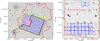 |
Fig. 1. Layout of the 91 fields observed for the MUSE-Wide survey in blue. Left: footprint in the Chandra Deep-Field South region overlaid on the V-Band image from the Garching-Bonn Deep Survey (GaBoDS; Hildebrandt et al. 2006). Shown in red are the approximate contours of the GOODS-S ACS and in yellow of the CANDELS-DEEP and HUDF09 parallels WFC3 regions. The magenta regions represent the nine MUSE-Deep intermediate depth mosaic of the HUDF. The current data release encompasses the fields enclosed by the thick black line. Right: footprint in the COSMOS region overlaid on the SUBARU-COSMOS i’-Band image (Taniguchi et al. 2007) available from IRSA (http://irsa.ipac.caltech.edu/Missions/cosmos.html). The red contours denote the southern tip of the deep HST exposures in the CANDELS-COSMOS region. |
Figure 1 shows the schematic mosaic tiling scheme of all fields in MUSE-Wide. The combined footprint of the 44 fields in data release 1 (DR1) is enclosed by the black line in the left side of Fig. 1. Adjacent fields have a nominal overlap of 4″ as a buffer for telescope pointing and offset errors. The candels-cdfs fields are oriented at a position angle (PA) of 340° to match the CANDELS-Deep field layout. For similar reasons, the hudf09-1 and hudf09-2 pointings were taken at a PA of 42° and 35°, respectively, candels-cosmos at PA of 0°, and the udf “shallow” again at 42°. Here we present and release the data for the first 44 candels-cdfs fields, that is, with field numbers 01–46. A future data release will encompass all 91+9 fields in both the COSMOS and CDFS areas.
2.2. Science goals
As a “blind survey of everything” within the survey footprint and sensitivity range, the design of MUSE-Wide clearly contains a strong legacy aspect. However, the choice of fields and the observing strategy were largely guided by our own scientific interests in these data, which we briefly sketch out in the following.
2.2.1. A spectroscopic sample of 1000 Lyman-α emitting galaxies
Already more than 50 years ago, the Lyα emission line of hydrogen was predicted to be a superb tracer for galaxy formation and evolution studies in the high redshift universe (Partridge & Peebles 1967). Meanwhile the study of Lyα-emitters (LAEs) provides a route to identify low mass galaxies at high redshifts that possibly constitute the progenitors of present-day L⋆ galaxies such as the Milky Way (Gawiser et al. 2007). Most LAE samples have so far been constructed from narrowband imaging (e.g., Hu & McMahon 1996; Rhoads et al. 2000; Ouchi et al. 2003, 2018; Shibuya et al. 2012; Sobral et al. 2017), but significant efforts need to be spent on confirming LAE candidates by spectroscopy. LAE samples have also been built from large multi-object spectroscopic surveys (Stark et al. 2010; Cassata et al. 2015), but in order to be efficient, such samples by construction rely on a very stringent photometric preselection of high-z candidates. The all-in-one approach of using MUSE as a survey instrument obviates the need of any pre-selection and follow-up spectroscopy. Given the typical surface number density of about ten LAEs detected per MUSE-Wide field (H17) we aim at building a sample of at least 1000 spectroscopically confirmed LAEs within 2.9 < z < 6.7, all located in fields with deep multi-wavelength data so that SEDs and physical properties can be studied. Initial results from our first installment of 24 fields include a measurement of the clustering properties of LAEs (Diener et al. 2017), an estimate of the Lyα emitting fraction among high-redshift galaxies (Caruana et al. 2018) and a determination of the Lyα luminosity function (Herenz et al. 2019). Already our first sample of 237 LAEs constituted one of the largest existing sets of high-z Lyα spectra, especially when demanding a spectral resolution good enough to study the line profiles in some detail (Gronke 2017).
2.2.2. Rare and extreme Lyα emitters
A small fraction of LAEs appears to have Lyα rest frame equivalent widths larger than the canonical limit of 200 Å for powering by stellar processes from populations seen in galaxies today (Kudritzki et al. 2000; Dawson et al. 2004; Gronwall et al. 2007; Kashikawa et al. 2012; Sobral et al. 2015; Hashimoto et al. 2017a). The reasons for such high equivalent widths are not well understood; a possible explanation could be a higher ionizing continuum and a consequently higher Lyα production rate at very low metallicities (Raiter et al. 2010), and/or the enhancement of Lyα emission in very recent bursts of star formation (Hashimoto et al. 2017b). The statistics of these extreme objects is still quite poorly known, but they have been posited to also be tracers for galaxies showing Lyman Continuum leakage (Dijkstra et al. 2016; Marchi et al. 2017). While measuring rest-frame equivalent widths higher than about 100 Å is very difficult using spectroscopy alone, the sensitivity can be greatly enhanced through the combination with deep broadband continuum imaging, especially from HST. Since most of the footprint of MUSE-Wide is within regions covered by HST data of several orbits depth, MUSE-Wide provides an exquisite dataset to search for LAEs with extremely high equivalent widths. At z = 3, associating a line flux of 2 × 10⁻¹⁷ erg s−1 cm−2 (well above the 5σ detection limit in most of MUSE-Wide) with an object of continuum magnitude of 28 in the AB system – roughly the 5σ limit in the ACS/F814W band of the GOODS-S images – would already imply a rest-frame equivalent width of ∼400 Å, measurable with high significance. Even Lyα equivalent widths of >1000 Å can still be measured confidently by combining MUSE-Wide with HST, and we will be able to set tight constraints on the occurence rate of such objects.
Another still enigmatic category of objects are the so-called Lyα “blobs” (LABs; Steidel et al. 2000; Bower et al. 2004; Nilsson et al. 2006; Weijmans et al. 2010; Erb et al. 2011; Matsuda et al. 2011), giant nebulae with often unclear associations to individual galaxies. Given the recent MUSE discovery that essentially all LAEs are also surrounded by extended Lyα-haloes (Wisotzki et al. 2016; Leclercq et al. 2017), a clear-cut distinction between “normal” haloes and genuine LABs may be hard to draw. It is yet unclear what the powering mechanism for LABs is; they could indeed be powered by diverse sources of energy, such as extreme star formation, cold accretion or AGN (Prescott et al. 2015; Ao et al. 2015; Trebitsch et al. 2016). Nevertheless, the scales associated with LABs make them different from the ubiquitous Lyα haloes around low-mass star-forming galaxies. With estimated comoving space densities between 10−6 and 10−4 per Mpc3 (Yang et al. 2011), LABs are moderately rare objects. The total survey volume of MUSE-Wide in Lyα amounts to roughly 106 Mpc3, large enough that we expect to discover several new LABs, all of them with already existing deep multiwavelength data.
2.3. Star-forming field low-mass galaxies at intermediate redshifts
Studying galaxies of stellar masses around or below ∼108 M⊙ is a difficult and expensive endeavour outside of the local universe. Even when restricting this to star-forming galaxies with strong emission lines, the extreme faintness of such objects makes them hard to find and even harder to constrain their properties. Yet such systems are of high astrophysical interest, as tracers of the continued build-up of stellar mass several Gigayears after the peak of the cosmic star formation history (e.g., Behroozi et al. 2013), but also as likely analogues to low-mass galaxies at higher redshifts, especially LAEs. In particular the so-called “green peas” (Cardamone et al. 2009) have recently captured a lot of attention, not least because of their possible relevance as leakers of Lyman continuum radiation (Izotov et al. 2016, 2018). Discovered by SDSS at redshifts z ≲ 0.3, most known green peas are however too bright and massive to be called genuine dwarfs. Shifting the known local population of blue compact dwarfs (BCDs) to z ∼ 0.5 would result in continuum magnitudes V ≳ 26, too faint for nearly all recent redshift surveys.
Such objects are, on the other hand, easily detected in MUSE datacubes from their conspicuous emission lines, as demonstrated by Paalvast et al. (2018), with ∼50% of the sample having stellar masses below 3 × 10⁸ M⊙. Again, MUSE-Wide provides an ideal hunting ground to find and characterise such systems, given the broad spectral range of MUSE and the huge amount of complementary data available. The wavelength range of MUSE complements blind HST grism surveys, which probe for these low mass galaxies at different redshifts and spectral resolutions (Atek et al. 2010; Maseda et al. 2018a). For the brightest galaxies of the sample, the 3D nature of MUSE data lets us build two-dimensional maps of the gas kinematics (Guérou et al. 2017).
3. MUSE observations and data reduction
3.1. Observations
The 44 candels-cdfs fields covered in this data release were observed in 12 GTO runs from September 2014 to March 2016 (see Table 1). Most fields (80%) were observed in dark time with seeing just under or around 1.0″. A more detailed description of the seeing properties is given in Sect. 3.2.5 when discussing the Point Spread Function (PSF) in the individual fields.
MUSE-Wide observation data.
Each MUSE-Wide pointing consists of 1h exposure time, split into 4 × 900s with 90° rotation in between and small fixed dithers between the single exposures. The four exposures did not have to be performed consecutively, they could be finished days later without any consequence to the later combination of exposures, except the varying observing conditions. The observations were carried out in nominal mode, meaning each spectrum spans from 4750 to 9350 Å in wavelength range, with the usual 0.2″ × 0.2″ spatial and 1.25 Å wavelength sampling, which is the default for MUSE. Most pointings did not have bright enough stars for the slow guiding system, hence we had to rely solely on the autoguider.
3.2. Data reduction
All data were reduced with version 1.0 or with an early development equivalent of the MUSE Data Reduction Software (DRS; Weilbacher et al. 2014). Although during the three years of observations of all MUSE-Wide fields newer DRS versions and ancillary software were released, we decided not to continuously update our pipeline, but to reduce all cubes consistently in the same manner. This ensured that quality differences are traceable solely to observing conditions.
The MUSE DRS operates in two stages. The first stage consists of calibration recipes which work on the individual CCDs to determine or remove the instrumental signatures of each IFU. At the end of this stage a pixel table is created, which relates each of the 24 CCD x−y positions and their flux values to a x−y−λ position on a datacube (Sect. 3.2.1). In the second stage one or several pixel tables are resampled onto a single datacube, usually with a 3D drizzling algorithm. We performed the first stage processes with the usual presets, but manipulated the pixel tables with our own routines before combining them into individual datacubes (Sect. 3.2.2). Furthermore, the combination of datacubes was also performed with our own procedures and we added some post-processing steps on the datacubes before arriving at the final datacubes (Sects. 3.2.3 and 3.2.4).
3.2.1. Basic pre-reduction
We produced the bias, flat, trace and dispersion master solutions from the standard set of calibrations taken at the end of the night for each MUSE-Wide observation. We applied these to the twilight skyflat observations from which we then produced a twilight cube, describing the unit-illumination correction.
After this, we applied the master solutions and the twilight flat to a standard star observation taken either at the beginning or at the end of the night. From these calibrated standard star exposures, we obtained the system response curve and telluric correction for each night. This response curve was further smoothed with a 30-order spline function to get rid of small scale wiggles due to instrumental defects or sparse sampling in the theoretical standard star spectrum. For each run we compared the response curves to each other and if there were no significant differences we used the response curve with the least instrumental defects for flux calibration in that run.
A new set of calibrations for the geometric and astrometric solution of the MUSE instrument was obtained during each ovserving run. After each science integration an additional illumination table (a short lamp flat) was taken. This additional flat-field accounts for the temperature variations in the flat-field, especially at the edges of the IFU. Using all these calibration data, we removed the instrumental signature from each CCD data and created the pixel tables.
We created a first version of a datacube for each exposure using the default values and the pipeline implemented sky subtraction. Using the collapsed whitelight images from these cubes, we calculated the WCS offsets by comparing a moderately bright star or two compact, moderately bright galaxies to their WFC3-F160W CANDELS HST position (see Fig. 2). This needed to be done for each exposure as the derotator wobble on MUSE introduced small offsets between exposures. Most of the WCS offsets were around 1″ and were primarily due to night-to-night telescope misalignment. The misalignment was especially pronounced in the beginning of November 2014 where the RA offset reached over 6″ (see candels-cdfs-04 in the exposure map in Fig. 4).
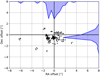 |
Fig. 2. Absolute RA/Dec offsets of the individual 15 min MUSE exposures to the CANDELS WFC3 160W coordinates (shaded in blue are the offset distributions). Most offsets are around 1″. |
Instead of applying the offsets during the cube resampling, we applied them to the reference World Coordinate System (WCS) in the pixel tables manually, by subtracting them from the header values. This later ensured that the four cubes had exactly the same sampling and could be combined without the need for drizzling. We did create a combined datacube using the WCS offsets, which was then our common output grid on which all four exposures were be resampled. Before we resampled, however, we applied our own sky subtraction and additional flat-fielding to the pixel tables described below.
3.2.2. Slice-based sky-subtraction
The sky subtraction implemented by the MUSE pipeline (Streicher et al. 2011) is good to about the 2% in areas outside of significant sky lines. However, the remaining sky emission line residuals are often significant and prevent us from reaching background-limited sensitivity, especially for wavelengths redder than wavelengths ∼7600 Å. Instead we developed an alternative method of sky-subtraction in MUSE data. Our approach works on the pixel table, so that further post-processing, such as the self-calibration routine described in Sect. 3.2.3 in the data reduction is possible.
The main idea behind the method is the self-similarity of the line spread-funtion (LSF) in the individual slices1 of the CCD image of each IFU. Since an emission line is sampled at just about two pixels in width in the wavelength direction in the CCD plane, the tilt of the slit and the curvature of the slices is crucial for the shape of the LSF. A line that occurs in the leftmost slice of the CCD will have a similar tilt and trace solution in all of the IFU CCDs. It is therefore not necessary to model the LSF previously, each sky line contribution is determined by an 24-IFU-average of the contribution from each of the individual 48 slices.
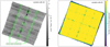 |
Fig. 3. Left: whitelight image of a single 15 minute exposure of a cube with only a few bright galaxies in the field (candels-cdfs-20), so that the contrast is enhanced. The dark regions in the slicer stack transitions immediately become visible. The regions in which the lowest 2% voxels are masked are marked by the green straight lines. Right: example of a collapsed, combined 4 × 900s exposure cube (candels-cdfs-01) showing the different exposure times at the edges due to the trapezoidal shape of the MUSE field of view. The square pattern shows the regions masked in the slicer stack transitions. |
First we masked out the brightest 15% and the dimmest 5% of regions in x−y datacube pixel coordinates (no WCS applied yet) to ensure bright objects or instrumental defects did not interfere with a pure sky spectrum. We created 48 “sky slice spectra” by taking the pixels from all 24 IFUs on one slice (about 6.5 million) and averaging in 0.2 Å bins, assuming that most of the slices contain empty sky and by aggressive sigma-clipping (2.0σ) to get rid of emission lines or cosmics.
In principle we now only had to subtract this “sky slice spectrum” by linearly interpolating it in wavelength and subtracting that interpolation value from each pixel flux value in the pixel table corresponding to that slice. Unfortunately the relative flux levels between each IFUs due to small differences in the flat-field, were significant enough to manifest themselves in the sky spectrum. These IFU-to-IFU flux differences were typically less than 2.5% in relative value (though this also depends on the location of the slice relative to the imaging edge), but were significant enough for the sky emission lines to show significant IFU-to-IFU discrepancies when subtracting.
We determined the relative flux levels for each IFU by fitting a Gaussian to three isolated sky emission lines ([O I] at 5577.338 Å and 6300.304 Å and OH at 8943.395 Å) across the spectrum for all 24 IFUs and all 48 slices in the pixel tables. While a Gaussian fit may not describe the emission line perfectly, we were only interested in the integrated flux, which to first order is conserved under changes of the LSF. We employed all the pixel flux values that lay within ±4 Å of the sky lines for the fit (≈550 per sky line). For each slice we then calculated the relative integrated flux values of the sky lines for each IFU and used the median value of these three to be the one to normalize the slice sky spectrum by for each IFU. This normalized, interpolated spectrum was then subtracted from each pixel flux value in the pixel tables.
In fact, the initial assumption that each slice has the same LSF is not strictly correct, hence there will still be residuals in the subtracted sky-line regions. However, the residuals using this slice-subtraction method are about 25% in amplitude when compared to v1.0 of the pipeline method. By working on the pixel tables, we could apply further post-processing steps described in the next section, including a second sky subtraction using principle component analysis (PCA). In addition, the sky normalization applied before subtracting can be interpreted as additional flat-field, ensuring greater uniformity.
3.2.3. Further post-processing in the data reduction
After we applied the slice-based sky-subtraction on the pixel tables, we used the MPDAF (Conseil et al. 2016) self-calibration method to remove systematic mean zero-flux level offsets between slices and IFUs. We employed whitelight images of each slice-subtracted pixel tables resampled to the common output grid as tracers for the mask applied in the self-calibration. We note that this early version of the self-calibration recipe (comparable to the one used on the HDFS; Bacon et al. 2015) still showed the familiar striping pattern in collapsed MUSE images. After we applied the self-calibration, we finally resampled the modified pixel tables one last time to the common output grid; each volume pixel in the datacube (voxel) had exactly the same 3D (RA, Dec, λ) position.
Because of flux aberrations in the slicer stack transition areas, some pixels at these transitions receive lower light levels, leading to dark spots in the combined datacube. These aberrations are wavelength dependent and are also seen to vary slowly over time. Since with the MUSE-Wide observing strategy each point in the sky ended up in four different IFUs and positions relative to the slicer stack, we dealt with this phenomenon as a cosmetic defect by a simple masking strategy. We masked out all the voxels that showed the lowest 2% of flux in the whitelight images and lay within the slicer stack transitions regions enclosed by straight lines (see Fig. 3a). When the four exposures were taken sequentially, there was little zero-point offset between the exposures, so the same straight-line regions could be used. Only when the exposures had significant pixel shifts with respect to the common output grid was there a need to set the masking regions manually.
Before we combined the masked cubes, we performed a second sky subtraction on the individual exposure datacubes to remove some after-residuals due to the varying shape of the LSF. We used ZAP v1.0 (Soto et al. 2016), a method taking advantage of the sky lines affecting all the voxels of the whole cube equally.
Finally we combined the four “ZAPed” individual 15 min datacubes. The flux cubes were averaged with a 3σ clip to exclude any extreme outliers known to be prevalent at the edges. The variance cubes were averaged (without sigma clipping) and divided by the square of number of exposures, capturing the masking and the different exposure levels at the edges. As explained below, the combined variance cube was subsequently replaced by a self-calibrated “effective variance” cube corrected for resampling (see Sect. 3.2.4).
We created a whitelight image by masked averaging over all the pixels of the flux datacube in wavelength direction. Finally, we created an exposure cube with values between 0 and 4 by summing up the individual exposure cubes, which consisted simply of a zero if there is a NaN value in the cube and one if there is not. The exposure cubes do not only capture the edges and the slicer-stack transition masking, but also masked out cosmic ray regions which only affect a small wavelength range or sparse coverage at the wavelength boundaries of 4750 Å and 9350 Å.
The two-stage sky subtraction procedure described above does a good job of keeping the background level reasonably flat within each spectral layer of a cube, especially across the instrumental stacks and slices, but it does not ensure a zero expectation value for the mean background level. We therefore added a postprocessing step to estimate background correction values as a function of wavelength. We first built a binary blank sky mask by thresholding the whitelight image, followed by a sequence of binary filtering (erosion and dilation), leaving typically ∼60% of the field of view as unmasked. We then calculate, separately for each spectral layer, the mean of all blank sky pixels. Assuming that the expectation value of the background correction in general varies slowly with wavelength, we smooth the array of mean background values by a succession of spectral median and Gaussian filters, which we then adopt as background correction for most layers. An exception is made at wavelengths with strong night sky emission lines and corresponding residuals, where we use the monochromatic mean per layer without the spectral filtering. The resulting background offset values are then subtracted from the cube. These corrections tend to be small, in the range of 2 × 10⁻²⁰ erg s−1 cm−2 Å−1, but would add up when integrating over large apertures.
All of these combinations were possible, because the individual cubes had the same astrometry and astrometric zero-point and had been resampled onto the same common output grid. The combined flux cube, the combined variance cube, the summed exposure cube and the whitelight image are all stored in a multi-extension FITS file. The multi-extension datacube for one field takes about 5GB of disk space. The cubes use air wavelengths (instead of vacuum) and are corrected to heliocentric reference frame.
Figure 4 shows a map of the collapsed exposure cubes (so-called “exposure whitelight images”) for the entire 44 fields (created with IRAF imcombine). Of particular note is the large WCS zero-point offset in candels-cdfs-04 and a large shift of two 15 min exposures taken four hours later in the night in candels-cdfs-25. Using the entire exposure map we compute the solid angle of the MUSE-Wide DR1 footprint with at least two 15 min exposures to be 39.5 arcmin2.
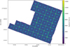 |
Fig. 4. Combined exposure maps of all 44 DR1 fields showing the coverage of the MUSE-Wide areas including the overlap regions which show up to 16 × 15 min exposures. |
3.2.4. Effective variances
The voxel-by-voxel variances obtained by formal error propagation in the MUSE pipeline systematically underestimate the true uncertainties in the cube because of the resampling needed to construct the cube, which shifts some of the power into covariances. Another disadvantage of the formally calculated errors is that they are inherently noisy, since they are based on actually measured count rates per voxel instead of the corresponding expectation values. This second property can lead to severe biases in the extraction of faint object spectra when using weighting schemes based on voxel variances. In H17 we tried to estimate the variances empirically by measuring the median aperture flux in 100 random empty sky positions in the MUSE flux cubes. We now describe an improved three-step procedure to replace the variance cube provided by the pipeline with empirically calibrated errors.
-
(i)
We measured, separately for each wavelength, the typical variance between individual blank-sky voxels as s2 ≈ [0.7413 × (q75 − q25)]2 where q25 and q75 are the 25% and 75% quartiles of the distribution of voxel values at given spectral layer and the factor 0.7413 rescales the quartile distance to an equivalent Gaussian standard deviation. These variance estimates implicitly include a contribution from small-scale systematics such as imperfect flat fielding or sky subtraction. To distinguish them from other approaches to quantify the uncertainties we denote these empirically calibrated errors as effective noise.
-
(ii)
To calibrate the bias arising from the resampling process we created an artificial pixel table with normally distributed random numbers with zero mean and unit variance and pushed it through the pipeline resampling with the same setup as the observational data, producing a cube containing only random numbers but including the cross-talk between neighboring voxels, thus with formally propagated voxel variances substantially smaller than unity. Assuming that the resampling effects on the variances are the same for this random numbers cube and for real datasets, we rescaled the empirical voxel-by-voxel variances s2 by a slightly wavelength-dependent calibration factor frs, λ (taken as the inverse of the median variance in the random cube) to approximately account for the losses due to resampling. We checked the correctness of this calibration by comparing the resulting effective noise values to the expected pure shot noise (without resampling) from the measured sky brightness and the detector readout noise, finding good agreement.
-
(iii)
We assume that at fixed wavelength the effective noise can be taken as a constant across the field of view, modulated only by the number n of independent exposures going into a given voxel (that is, the exposure cube, see Fig. 3b):
 . In other words, we assume the data to be strictly background-limited and neglect the enhanced photon shot noise in real objects for the estimation of the errors. While this implies somewhat underestimated variances in the central pixels of bright sources, it is an optimal assumption for faint objects where robust error estimates are most important for detection and measurement purposes.
The 44 final released datacubes contained in the Data Release 1 (DR1) have all been background-subtracted and the empirically calculated effective noise has been inserted instead of the variance noise scaled by the exposure cube. We release the individual MUSE-Wide datacubes as a combined “44-field” datacube would have been too large and inconvenient for further analysis both in terms of computer memory and computation speed.
3.2.5. Estimation of the point spread function in the final datacubes
One important characterization of the datacubes is the estimation of the point spread function (PSF). The Gaussian FWHM that the Autoguider star measurement provides is only a rough approximation. Optimal spectral extraction of compact sources requires good knowledge of the MUSE PSF (see Sect. 5.2). Similarly, for the detection of emission line sources using a matched filtering approach, we require the PSF for cross-correlating with our model images (see Sect. 4.1). In addition, the large wavelength range covered by MUSE required taking the variation of the PSF shape with wavelength into account.
The MUSE PSF has been shown2 to be well characterized by a Moffat circular function (Moffat 1969):
 (1)
(1)
where Σ0 denotes the central intensity, the width of the profile is mainly determined by the dispersion radius rd, while the β-parameter defines the kurtosis of the profile. The full width half maximum of the Moffat profile can then be expressed in terms of rd and β as 
A theoretical description of wavelength dependence of the PSF broadening has been derived in the framework of the Kolmogorov turbulence model of the atmosphere (e.g., Tokovinin 2002), but for our purposes the decrease of the FWHM with wavelength can be approximated with a linear function. We opted to keep the Moffat shape parameter β constant over the MUSE wavelength range; previous experience has shown its variations to be negligible (Kamann et al. 2013). We defined the reference wavelength to be at 7050 Å, at the center of the MUSE wavelength range and for comparison with the Autoguider measurement:
![Mathematical equation: $$ \begin{aligned} FWHM(\lambda )[^{\prime \prime }] = p_0 + p_1(\lambda - 7050\,\AA ). \end{aligned} $$](/articles/aa/full_html/2019/04/aa34656-18/aa34656-18-eq4.gif) (2)
(2)
In addition to the Moffat, we also computed the Gaussian profile of the PSF, which misses its outer wings, but is in many ways easier to handle. As for the Moffat, we assume circular symmetry for the Gaussian representation, so that the PSF is fully described by its FWHM, which also varies with wavelength according to Eq. (2), albeit with different p0 and p1 factors.
We used altogether four different methods to estimate and model the PSF in the combined datacubes, with some changes after completing the first set of 24 fields. When multiple methods were available we always selected the result that appeared most reliable, with the Gaussian FWHM measurements obtained by the VLT Autoguider during the observations as an additional independent check.
-
Method P: Direct PSF fitting of stars in the field of view using PAMPELMUSE (Kamann et al. 2013). While a priori this seems the cleanest way to obtain the PSF, the stellar surface density in the CDFS is so low that less than 30% of the fields contain at least one sufficiently bright star (mF814W ≲ 22.5). We modeled the PSF in MUSE collapsed mediumband images of 1150 Å width, that is, for four wavelength bins, and then obtained the values of p0 and p1 of Eq. (2) by fitting a linear function to the wavelength dependent FWHM.
-
Method G: Inferring the PSF from modeling compact galaxies. We visually selected from the HST/ACS F814W images relatively bright, compact galaxies without much structure, which we then convolved with a grid of different PSFs to match the MUSE resolution. The convolved and downsampled images were compared with MUSE collapsed mediumband images of 125 Å width, and the best-match PSF parameters were then determined by minimizing χ2 over the grid, for each wavelength bin. p0 and p1 were again obtained by fitting a linear function in wavelength. This method was only used to obtain Gaussian PSF parameters for fields 01–24 and was later replaced by method C.
-
Method C: A hybrid method combining stars and compact galaxies. In order to go as faint as possible we modeled the PSF in only two broadband images corresponding to the HST/ACS bands F606W and F814W, which together cover the MUSE spectral range almost perfectly. Objects that proved difficult to model were excluded. The linear relation parameters p0 and p1 followed directly from the two broadband models. The method was applied to fields 25–46 to obtain both Gaussian and Moffat PSF parameters.
-
Method F: Full-frame modeling using the fast Fourier transform (FFT) method described in Bacon et al. (2017), applied to the comparison of HST and MUSE F606W and F814W broadband images. While potentially most powerful, this approach suffers from the need to exclude all stars with measurable proper motion between the HST and MUSE observation epochs (that is, exactly those objects providing the best PSF constraints). We applied this method to estimate Moffat PSF parameters for all fields in this DR1, but in several cases (especially when there were stars in the field) the results from method C appeared more robust and were preferred.
Table 2 documents which method was finally used for which parameter set. Figure 5 shows an example of the different FWHM determined as a function of wavelength for both the circular Moffat and Gaussian parameters. Similar figures of the PSF determination are found in the Quality Control pages of the data release webpage for each field (see Appendix A).
Moffat and Gaussian PSF parameters chosen to describe the PSF.
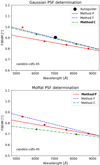 |
Fig. 5. Example of determined PSF slopes for the various methods on the field candels-cdfs-45: in the upper panel for the Gaussian p0 and p1 values and in the lower for the Moffat values. Methods (as described in text): P = direct fitting of stars, C = hybrid method of fitting stars and galaxies combined, F = Fast Fourier Transfrom. The final selected method is marked in bold letters. |
4. Emission line selected objects
MUSE can efficiently locate sources in a 3D cube without any photometric pre-selection; it is particularly powerful for the detection of emission line objects. Most of the science cases of MUSE-Wide rely on emission line sources detected in a homogeneous manner (Sect. 2.2). In H17 we provided a catalog of 831 emission line sources for the first 24 fields of MUSE-Wide using a matched filtering approach. Since then we employed the same strategy for the other 20 fields of the MUSE-Wide DR1. Here we only provide a brief description of the process already described in H17.
4.1. Detection and classification
Prior to searching for emission lines in the datacube we had to remove any underlying continuum signal from the specta. To achieve this goal we subtracted a 151 pixels wide running median in spectral direction from the datacube. The continuum-subtracted cube was then fed into the LSDCat software (Herenz & Wisotzki 2017), together with the empirically determined “effective variances” (Sect. 3.2.4). In brief, LSDCat cross-correlates the entire cube with a 3D source template and provides a list of emission line detections graded by significance. For the spatial template we adopted for each field a circular Gaussian with a FWHM of the PSF (Sect. 3.2.5), thus targeting in particular compact emission line sources. For the spectral template we took again a Gaussian, but with a FWHM fixed in velocity space to a value of 250 km s−1, a value optimised to find Lyα emitters. However, the algorithm is quite robust against template mismatches (see discussion in Herenz & Wisotzki 2017).
In order to define candidate emission line detections, LSDCat requires a detection threshold in the signal-to-noise ratio (S/N). In comparison to H17 we lowered this S/N threshold to a value of 5.0, which turned out to be as low as we could go before getting strongly affected by spurious detections (see below). We note that this lower threshold applies only to the newly added fields, while the detection limit for the first 24 fields was 8.0 in S/N using the old recipe for the effective variances, which converts into a value of 6.4 with the new improved prescription3. On output, LSDCat groups multiple line detections together that were found within a certain radius (which we set to 0.8″). A candidate object thus consists of one or several detected lines, where the detection with the highest S/N is denoted as “lead line”.
In the next step we visually inspected and classified all detected objects with our QtClassify tool4 (Kerutt 2017) in a two stage process: In a first pass, each object was classified independently by two team members, followed by a second pass where these two and a third member as referee had to agree on the final classifications. The referee had final say on cases in which the initial classifiers disagreed. During the inspection process we purged spurious sources such as sky or continuum subtraction residuals, classified the remaining objects by identifying the lead line (and thus setting the redshift), and assigned qualitative indicators describing the robustness of the classification. For the latter we distinguish between “quality” and “confidence”: Quality specifies whether any secondary lines have aided the classification process (“A” for multiple lines above the S/N threshold, “B” if only one line was detected, but more are visible in an extracted S/N spectrum and match in redshift, and “C” for single-line objects). The “confidence” value is a more subjective interpretation of our trust in the classification, with a value of 3 expressing very high certainty, 2 representing a still quite trustful result (expected error rate ≲10%), and 1 the lowest confidence with an assumed error probability in the correct identification of the line of up to ≈50%. Also here the referee in the second classification pass had final say on the quality and confidence indicators in the catalog, especially when the two initial classifiers did not agree. Even with multiple classification passes, some degree of subjectivity remained, particularly at the boundaries.
We emphasize that the leading emission line detection of confidence 1 objects is still highly significant, and we expect a low rate of entirely spurious detections. Comparison of the MUSE-Wide emission line catalog in the UDF with the MUSE-Deep catalog utilizing the full ten hour exposure time (Inami et al. 2017), yielded ≈5% false positives and all were at a S/N level less than 6. We will explore the comparison of the shallow MUSE-Wide survey versus MUSE-Deep further, when we release that portion of MUSE-Wide in a future Data Release 2. The lower confidence mainly reflects the ambiguity of the line identification, not the fidelity of the source itself. Figure 6a shows the distribution of S/N values of the lead emission line for the three different confidence levels; our confidence level clearly depends strongly on the S/N of the lead line.
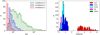 |
Fig. 6. Left: distribution of number of emission-line objects as a function of S/N of the lead line for each of the three confidence levels we employ for classification. Objects at the S/N limit are dominated by confidence 1 objects and may include some spurious lines, while for objects with S/N above 10, we expect hardly any misclassifications. Right: redshift histogram of the emission line sources classified by their strongest line. The redshift desert, where there are no strong emission lines in the MUSE wavelength range between 1.5 < z < 2.9, is clearly visible. We are able to find 479 LAEs, reaching densities of almost 12 LAEs/arcmin2. |
While LSDCat and QtClassify already yielded provisional redshifts, these were subsequently refined as follows: We extracted PSF-weighted one-dimensional (1D) spectra at the position of the emission line source, with both air and vacuum wavelengths using the Vienna atomic line database formalism (Ryabchikova et al. 2015)5. Lyα-based redshifts were then based on the peaks of fitted line profiles assuming an asymmetric Gaussian line shape (Shibuya et al. 2014), with however no correction for any offset the Lyα line from systemic. Redshifts for other emission line galaxies (z < 1.5) were determined by fitting Gaussian line profiles simultaneously to all emission lines present in the object. For the [O II] doublet we used a double Gaussian with fixed separation, all other lines were fitted with single components. The final redshift was taken as the S/N-weighted mean of all lines, and redshift errors were estimated by repeating the fitting procedure 100× on the spectra after randomly perturbing them according to the effective noise.
Following classification we created a merged object catalog for the entire DR1 footprint. We discarded double detections in overlapping regions of adjacent MUSE-Wide fields (always retaining the detection with higher S/N). We also had to perform some manual interventions such as grouping emission line sources belonging to the same galaxy, but which was too extended for the automatic grouping of LSDCat, and splitting up superpositions of different-redshift emission line objects closely aligned in the line of sight. After merging and cleaning we were left with a final catalog of 1602 emission line objects, based in 3057 detected emission lines. The redshift distribution of the objects, grouped by their lead-line identifications, is shown in Fig. 6b. This plot shows a clear redshift desert between z ≃ 1.5 (where [O II] is redshifted out of MUSE) and z ≃ 2.9 (where Lyα enters); the region in between is populated only by two AGN. We note that the continuum-selected sample discussed in Sect. 5 does not have such a redshift desert (see also Fig. 14). Figure 7 shows a montage of all 1602 emission line object spectra stacked in y direction with increasing redshifts.
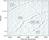 |
Fig. 7. Stack of normalized spectra of the emission line objects. They are stacked in y-direction with increasing redshifts, with a large jump between z∼1.5 and z∼2.9. First we normalized the spectra to the brightest emission line, then we smoothed with a 10 Å Gaussian and finally we smoothed the 2D image with a 2.8 pixel 2D circular Gaussian. |
The released data tables (object catalog and emission line table) are described in Sect. 4.4 below. Here we briefly introduce the unique identifiers of MUSE-Wide emission line objects, UNIQUE_ID in the catalogs. It is composed of nine digits and divided into four groups in the format “ABBCCCDDD”. The first digit refers to one of the five parent regions in which the MUSE pointing was obtained (which is always 1 in DR1, for candels-cdfs). Next comes the two-digit number characterising the field in which the object was discovered. CCC refers to the LSDCat object identifier in that field, and DDD refers to the emission line running number for the lead line in the emission line table. The last number is important for distinguishing superpositions of objects at different redshift that were assigned the same object ID by LSDCat. Thus for example, the source with unique identifier 106043096 was found in field candels-cdfs-06 as LSDCat object 43, and its lead line has the running number 96 in the emission line table.
4.2. Cross-match with photometric and spectroscopic catalogs
By cross matching the MUSE emission line objects to multiband HST catalogs we could add broad band photometry, especially far into the near-IR wavelengths unaccessible with MUSE. For the cross-match we use two catalogues currently available in the CANDELS/CDFS region: the Guo et al. (2013) CANDELS catalog based on deep F160W WFC3 imaging and the Skelton et al. (2014) 3D-HST catalog based on a combination of the F125W/F140W/F160W WFC3 filters. While the 3D-HST catalog is deeper, it shows higher fragmentation of sources at low redshift. Also, while the 3D-HST offers excellent and vast photometry, particularly in the near-IR data, the CANDELS catalog provides more complete links to other multiwavelength information, such as X-ray and radio.
We determined the photometric counterparts to our emission line sources by searching for the nearest counterpart within 0.5″. In H17 we had estimated the 3σ positional error between the HST catalogs and the MUSE LSDCat position of the emission lines to be <0.5″. We then visually inspected the HST image cutouts and consolidated the counterpart list, either by adding potential counterparts outside 0.5″ or by purging the closest catalogued counterpart if it did not match our expectations of the emission line (for example, no drop in the broad band images representing the rest-frame Lyman continuum for a Lyα-emitter).
Table 3 shows the percentages of MUSE counterparts found in the two photometric catalogs. As expected, we are nearly complete at low redshift, the main source of incompleteness being superpositions with large galaxies. At high redshift, the LAEs show a much lower percentage of photometric counterparts. In some of those sources we find a clear counterpart in the optical HST images, but they are not catalogued in the near-IR selected catalogs, possibly because of their UV-dominated spectra energy distribution (SED). Other high redshift sources are just below the detection limit of the broad-band images, hence the higher percentages of LAE counterparts in the deeper 3D-HST catalog. As in the MUSE deep fields, also here we detect several LAEs without any photometric counterparts, neither in the images nor catalogs (Maseda et al. 2018b; Bacon et al. 2017); these constitute some of the highest equivalent width sources known (EW0 > 500 Å) and will be the subject of further study within MUSE-Wide (Kerutt et al., in prep.). Lastly, some of the LAEs without counterparts at very low S/N and low confidence may be spurious detections within MUSE and not real sources, but we estimate that fraction to be ≲5%.
Counterpart percentages between the emission line sources to HST selected catalogs.
We also compared the 1355 emission line galaxies with 3D-HST (Brammer et al. 2012) counterparts to their redshift measurements from the literature. Although the CANDELS team has an internal photometric redshift selection combining six photometric redshift (photo-z) codes following the study of Dahlen et al. (2013), only one of those photometric redshift determinations is public (Hsu et al. 2014). We opted to wait until the CANDELS collaboration releases their photometric redshifts to compare the MUSE spectroscopic redshifts to them. The bulk of the 3D-HST redshift measurements came from Skelton et al. (2014) using the EAzY code (Brammer et al. 2008) to determine their photometric redshifts. EAzY benefits from the large amount of photometric bands that 3D-HST provides. Furthermore Skelton et al. (2014) included previous spectroscopic redshifts from their study (see Wuyts et al. (2008) for a compilation of the different spectroscopic campaigns used). We added 330 mostly low redshift sources with updated HST grism spectroscopy from Momcheva et al. (2016). The changes between the Skelton et al. (2014) photometric redshifts and the grism redshifts are minimal, since the grism identification is aided (and often dominated) by the photo-z. We furthermore added 22 sources with new spectroscopy from the VIMOS Ultra-Deep Survey (VUDS) (Le Fèvre et al. 2015; Tasca et al. 2017) to our comparison for a total of 307 objects with spectroscopic redshifts (not counting the 330 grism redshifts).
Figure 8 shows the comparison between our spectroscopic classification and various redshift values from the literature, including a majority of photometric redshifts from Skelton et al. (2014). There exists a systematic offset between the photometric and spectroscopic redshifts for our high redshift LAEs when there is not a catastrophic redshift failure, with the median offset between the MUSE redshift and the 3D-HST photo-z being Δz ∼ 0.2. This offset has been remarked upon by Oyarzún et al. (2016) and most likely relates to EAzY shifting a slightly blueshifted Lyman break when strong Lyα emission is present to account for the flux excess in the redder band. An extensive investigation into the sources of mismatch between MUSE spectroscopic redshifts and photometric redshifts was studied by the MUSE-Deep survey (Brinchmann et al. 2017). In addition to the template mismatch in EAzY noted above, the authors explain that a source of further contribution to the offset at high redshift relates to the amount of intergalactic absorption these high redshift galaxies experience. They also find, perhaps counterintuitively, that adding extensive ground and mid-IR photometry to very faint sources worsens the photo-z prediction. Lastly, they remark that a wrong association can play a significant role, which we also find when comparing our sources with spectroscopic samples below.
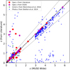 |
Fig. 8. Redshift comparison between MUSE and literature redshifts for our emission line selected galaxies. Red dots denote the compilation of redshifts from the literature gathered in Skelton et al. (2014). Magenta hexagons represent spectroscopic measurements from VUDS (Tasca et al. 2017). Green crosses represent grism spectroscopic redshifts from Momcheva et al. (2016), which were aided by the photometric redshifts from Skelton et al. (2014) denoted with blue crosses. The thin dashed lines show the regions outside of which a photometric redshift is determined as a catastrophic failure. |
We defined a catastrophic redshift failure between literature and MUSE redshifts to occur if the following condition was met for photometric redshifts:
 (3)
(3)
and |zspec − zMUSE|> 0.1 for spectroscopic redshifts. 113 objects (8% of 1355 emission line objects) satisfy those conditions, with the majority (101) coming from catastrophic photometric redshift errors. We investigate the 12 mismatches between literature spectroscopic redshifts and MUSE spectroscopic redshifts in Table 4. Except for object 137012028, which shows a photo-z probability distribution function matching better to the high redshift solution, we are quite certain in our classifications of the sources, often having other lines or spectral features to aid us in our assessment of the redshift.
Catastrophic failures for objects with spectroscopic redshifts from the literature.
4.3. Stellar masses
We also determined the stellar masses of the emission line objects with a catalogued photometric counterpart. SED derived stellar masses carry many uncertainties, for example, the proper accounting for emission lines. We caution that the stellar masses derived serve only as an estimate. We used the Skelton et al. (2014) photometry and the software FAST (Fitting and Assessment of Synthetic Templates; Kriek et al. 2009) similar to the 3D-HST team, allowing for an easy comparison between the samples. FAST determines the best fit parameters using χ2 minimization from a set of model SEDs and an analysis grid describing several stellar population models.
The stellar population model grid parameters are: stellar age, characteristic star formation timescale τ, dust content AV, metallicity and redshift (which we fixed to the MUSE redshift). As in Skelton et al. (2014), we employed the Bruzual & Charlot (2003) stellar library, the Chabrier (2003) initial mass function and the Calzetti et al. (2000) dust law for our fits. For low-redshift sources (z < 2.9) we used an exponentially declining star formation history, where τ refers to the width of the declining exponential, while the stellar age is when the star-formation burst happened before the exponential decline. However, for our high redshift LAEs this model is likely unphysical, since the galaxies are going through a young burst, which is possibly their first and dominates the continuum of the sources. Using a truncated star formation history in which τ corresponds to the length of the burst and is equivalent to the age improved the χ2 of the fits dramatically, even if they could not capture ages below 40 Myr in the models. We expanded and refined the analysis grid of Skelton et al. (2014) slightly, for example employing finer steps for the stellar ages, dust attenuations and using 4 metallicities (0.004, 0.008, 0.02 and 0.05 Z⊙) instead of just one (0.02 Z⊙) used by Skelton et al. (2014). Once a preferred stellar model was found, stellar masses were derived via the mass to light ratios of that model adjusted to the SED photometry.
Figure 9 shows the distribution of the thus obtained stellar masses of emission line galaxies, divided into high and low redshift subsets. Both distributions are fairly broad, but show a significant tail toward low mass, dwarf systems; 55 LAEs have stellar masses lower than log(M⋆/M⊙) = 8.0, while 59 intermediate redshift galaxies have masses lower than log(M⋆/M⊙) = 7.5. The LAEs typically have lower masses than other galaxies, such as Lyman Break Galaxies (LBGs) found at these redshifts. However, this is just a consequence of the selection method; the need for photometry skews them to have higher stellar masses (Hagen et al. 2016). At intermediate redshifts, MUSE-Wide is able to peer into the field population of star forming dwarfs. If emission lines were included in the SED fitting the steller masses would likely decrease for both samples, further emphasizing that this emission line catalog skews toward low mass systems.
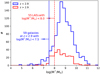 |
Fig. 9. Stellar mass histogram for emission-line objects with photometric counterparts, in red for high-redshift LAEs, in blue for lower redshift objects. We find a tail of low mass dwarf galaxies representing some of the lowest mass galaxies known at these redshifts. |
We do not provide age estimates, dust attenuation or star formation rates (SFR) derived from the stellar models as these SED derived parameters have been shown to contain large uncertainties and should be dealt with on a case-by-case basis taking into account emission line strengths for their analysis (e.g., Stark et al. 2013). On average, though, LAEs are known to have extremely young populations with a large fraction hitting the 40 Myr limit and specific star formation rates lying well above the high redshift main sequence (Speagle et al. 2014).
In Fig. 10 we compare our derived stellar masses with the ones from Skelton et al. (2014). The largest differences in the stellar mass estimates come from catastrophic failures for the redshift estimation from photometric data, so we display them with blue triangles and do not take them into account for our statistics. As the plot shows, the unlikely stellar masses of log(M⋆/M⊙)≪5.0 in the Skelton data are due to the galaxies being assigned an incorrect, much lower redshift than they actually have. At low redshifts we find good agreement between the stellar masses where there are no catastrophic redshift failures, with a standard deviation of the differences between the masses of 0.11 dex. At high redshifts, the scatter is larger, here the standard deviation of the differences between the stellar masses is 0.28 dex with some stellar mass differences almost reaching 1.0 dex. This is understandable as the photometry has larger errors for these fainter sources, hence the probability distribution functions for the χ2 minimization will be broader. Furthermore, also here redshift errors play a role, in particular the systematic shift of Δz ∼ 0.2 already noted can introduce an overestimate of ∼0.1−0.15 dex (Nanayakkara et al. 2016).
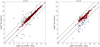 |
Fig. 10. Photometric mass estimates fixed at the MUSE-Wide spectroscopic redshifts compared to the Skelton et al. (2014) photometric mass estimates based on photometric redshift estimates. The solid line represents the 1:1 mass equivalency, while the dashed lines show ±1 dex differences between the two stellar mass estimates. Marked with blue triangles are catastrophic redshift outliers, which will be the main cause of discrepancies. At low redshift there is good agreement between the stellar masses, while at high redshift the scatter between the masses is larger due to the large photometric errors associated with these faint galaxies. |
4.4. Final emission line catalogs
Similar to H17, we created two catalogs from our emission line search. One is an object catalog in which the information (redshift, confidence, photometric counterparts, etc.) for the emission line galaxy is stored. Its UNIQUE_ID is determined by the leading emission line as described above. The other is an emission line catalog, which is cross-referenced to the object catalog through the UNIQUE_ID. In it the physical properties of all emission lines (coordinates, extent, flux, etc.) are listed, including all secondary lines associated to an object.
In addition to the 1D PSF weighted spectra (see Sect. 4.1), which are optimized to provide the best S/N in the emission lines, we also extracted aperture spectra with the Kron radius as the aperture radius (with a lower limit for the radius of 0.6″). While these spectra tend to be noisier, as they include regions that are not strongly line-emitting, they capture the spatially extended flux of the emitting galaxy withot a bias toward the emission line region. Most of the emission line galaxies are more extended than the PSF, hence the aperture spectra are more realistic representations of the flux emanating from the emission line galaxy as a whole. As in H17, both PSF weighted and aperture spectra are stored as FITS binary tables with columns for both air and vacuum wavelengths.
The catalogs and spectra are available on the MUSE-Wide data release webpage6 (see Appendix A.2). The main emission-line source catalog includes links to subpages, which include images centered at the emission line position, a link to download the two 1D spectra described above, a cross reference to the Guo et al. (2013) cross-matched subpage (see Sect. 5) and a link to download a 6″ × 6″ mini 3D MUSE cube centered on the emitter position. The entries and formats for the different catalogs are described in the “Database” tab of the MUSE-Wide webpage (see Appendix A.4), but are similar to the catalog entries of H17 except for the addition of two columns, one for a MUSE-Wide field identifier and one for the stellar mass of the object (described in Sect. 4.3).
4.5. Cross-match with other multiwavelength catalogs
4.5.1. X-ray
We then cross-matched our emission line objects with the X-ray source catalog from the CDFS-7Ms Chandra observations (Luo et al. 2017), the sources of which, are dominated by AGN. Traditionally blind emission line surveys have unveiled numerous active galaxies, so we expect some of the MUSE-Wide emission line galaxies to contain AGN, too. At redshifts z < 0.4, where Hα and other optical emission lines fall within the MUSE wavelength range, we can employ the BPT diagram (Baldwin et al. 1981) to distinguish AGN from star-forming galaxies. At higher redshifts, however, we either need to resort to other classification schemes (which are however more ambiguous, e.g., Juneau et al. 2011) or perform expensive near-IR spectroscopy to obtain the rest-frame optical lines. X-ray data can help in distinguishing the galaxies, particularly if the source is X-ray luminous. Some weak X-ray sources can be driven by star-formation, but their signal is of low luminosity and very soft, as it represents the energetic tail of a thermal signal.
A cross-match was achieved when an emission line source is within three times the X-ray positional accuracy (SIGMAX in Table 4 of the Luo et al. 2017 catalog). In H17 we required the X-ray source to be luminous (have an “AGN” flag associated with it); we drop that requirement as to classify even the faintest X-ray sources as they may be at high redshift. One of the goals of extending the X-ray imaging in this field to such long integration times was to find intermediate and low luminosity AGN at high redshift for investigating the faint end of the AGN luminosity function at z > 4. This may provide clues about the relative contribution of quasars to the reionization of the Universe (Giallongo et al. 2015), and could also constrain the earliest growth periods of black holes (Weigel et al. 2015).
We match 127 emission line sources to X-ray counterparts after purging two superpositions from the X-ray catalog. As there have been extensive campaigns to identify the X-ray sources since the CDFS began observing in the early 2000s (for example, Szokoly et al. 2004; see Luo et al. 2017, for the 26 literature references used for spectroscopic redshift determination), it is not surprising that most of the sources have a spectroscopic redshift associated with them. We are nevertheless able to assign spectroscopic redshifts to sources which previously only had photometric redshifts. All but six spectroscopic redshifts and two photometric redshifts are in excellent agreement with each other. In some cases, when the separation between the sources is large, the spectroscopic redshift may refer to another object and in other cases there may be a misidentification of the spectrum. The discrepant cases and the newly identified sources with only photometric redshifts are listed in Table 5, marked S14/H14 for new identifications (10) and zSpec for redshift discrepancies (6). We note that the two high redshift MUSE-Wide sources marked with stars are not associated to the optical counterpart for which the photometric redshift was derived and due to their large distance to the X-ray source are likely not associated with it either.
Table of matched X-ray objects with only photo-z values or disagreement between the redshifts.
Perhaps surprisingly we did not identify any new high redshift (3 < z < 6.5) sources in the X-ray population with our emission line sample. The only two emission line sources above redshift of 3.0 are well known Type 2 QSOs (MUSE-WIDE IDs: 104014050, 115003085), both of which have the highest Lyα fluxes in our survey (Norman et al. 2002; Mainieri et al. 2005). In the future we plan to match the X-ray catalogs also to non-emission line sources and blindly extract MUSE-spectra at the X-ray position to peer further into AGN demographics at high redshift, but that is beyond the scope of this paper.
We may, however, characterize possible AGN emission from our high redshift LAEs to determine whether there is low luminosity X-ray activity coming from that population. Previous studies (Treister et al. 2013; Vito et al. 2016) have explored the possibility of identifying early black hole growth by stacking several high redshift galaxies in the CDFS. AGN at high redshift are less affected by obscuration as the high energy window moves into the Chandra spectral range. While Treister et al. (2013) did not find any signal among luminous LBGs, Vito et al. (2016) found a significant X-ray emission from massive galaxies at z ≈ 4, however attributing it to mainly star formation processes. They speculate that since they did not find dominant AGN features, either the dominant AGN population is in fainter galaxies, the processes are hard to see or that most of black hole growth occurs at later times in the Universe. This also implies a flattening of the AGN X-ray luminosity function at high redshift.
Having a sample of 477 fainter high redshift sources at hand (479 LAEs minus the two QSOs mentioned above), we also stacked the corresponding CDFS X-ray data. We used CSTACK7 (Miyaji et al. 2008) a web-based stacking tool, which takes into account the intricacies of exposure maps, response matrices, PSF variations, etc., for various deep Chandra fields. At the time of the analysis the 7Ms data (Luo et al. 2017) was not yet freely available on the CSTACK interface, so we use the 4Ms data (Xue et al. 2011) for stacking, yet a subsequent stacking analysis done by scientists with access to the 7Ms data yielded similar results (Vito, priv. comm.).
Figure 11 shows the results of the X-ray stacking. The mean count-rate for both the low and high energy band is consistent with zero. The combined stack has a 3σ upper limit of 2.8 × 10⁻⁸ cts s−1 or 3.6 × 10⁻¹⁸ erg cm−2 s−1 in X-ray flux8. The population of LAEs does not show any AGN activity in the stacks and is therefore not dominated by it, at least not by typical accretion processes, which produce an X-ray corona. Either black hole growth is a stochastic process occurring only in a small fraction of galaxies in the early Universe leaving the bulk of the black hole growth to happen at a later time or the processes are radiatively inefficient and/or heavily obscured, for example, super-Eddington accreting Broad Absorption-Line Quasars which are X-ray weak (Luo et al. 2014).
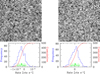 |
Fig. 11. Null result of stacking X-ray images from the 4Ms CDFS data at LAE positions. The panels on the left refer to the soft band (0.3–2.0 keV), the ones on the right to the hard band (2.0–7.0 keV). Upper panels: stacked images, whichare 20″ × 20″ interpolated on a 0.5″ pixel size Chandra grid. Lower panels: statistics of the mean stack. |
4.5.2. Submillimeter and radio
An interesting question is whether LAEs can be related to submillimeter galaxies, which are also forming stars at a high rate or host AGN, but usually belong to a far dustier population of high-redshift sources. Unfortunately, of all the continuum submillimeter sources catalogued with ALMA in the CDFS in the ALESS survey (Hodge et al. 2013) only one falls within the fields of view of MUSE-Wide DR1. ALESS 10.1 is in candels-cdfs-05, is centered on CANDELS # 4414 and also matches the X-ray source 342 of Luo et al. (2017; see Fig. 12). There is no match to our emission line catalog (MUSE-Wide 105011043 is nearby, but is clearly attributed to another galaxy). The source shows has a steeply rising SED all the way out to the mid-IR without any noticeable breaks from the broad band filter fluxes. Hsu et al. (2014) assign a photo-z of z ∼ 0.76 to the source, but we cannot confirm this from our optimally extracted spectrum of that source (see Sect. 5.2) as it shows no identifiable spectral features.
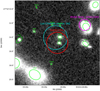 |
Fig. 12. CANDELS WFC3 6″ × 6″ cutout of the region centered on ALESS 10.1. CANDELS photometric objects from Guo et al. (2013) are marked in green, a MUSE-Wide emission galaxy with a 0.8″ radius in magenta, the X-ray source with its corresponding error radius in cyan and the ALESS source with an arbitrary 1.5″ radius in red. |
As with X-ray sources, radio surveys are ideally matched to emission line surveys, because the physical conditions that produce radio emission (synchrotron emission for AGN, thermal free–free emission from star-forming HII regions) also may produce emission lines. We cross-match the 464 sources from the Very Large Array (Jansky Array; VLA) 1.4 GHz survey over the extended-CDFS (Kellermann et al. 2008; Miller et al. 2008) to our emission line sources. As radio positional errors were small (≲0.2″), we used a fixed 1.0″ as our matching radius. 11 radio sources match and all but one of the matches to the emission line catalog are also X-ray sources listed in the Luo et al. (2017) catalog. All have previous spectroscopic identifications in the Literature and all but one agree with the MUSE-Wide redshifts (see Table 6). The redshift mismatch belongs to MUSE-Wide source 146002220, which has only confidence 1, its S/N is very close to the limit of 5.0 and it may not be associated to the correct source (see also Table 5). The much closer source to the X-ray and radio position is CANDELS ID #16375. It does not fall in our emission line catalog and we are only able to identify it as a z ∼ 0.442 galaxy with confidence 1 (see Sect. 5.3).
Emission line sources match to VLA radio catalog.
5. Spectroscopy and identification of photometrically selected objects
One of the advantages of the concept of “spectra of everything” is that we can actually extract a spectrum “of everything” even if at the end it is too noisy for identification. A MUSE extraction showing a noisy spectrum for a specific photometric object at least tells us that the object does not have strong emission lines or other spectral features, so that any future follow-up will require substantially higher integration times. We decided to first concentrate on the CANDELS Guo et al. (2013) catalog for spectral extractions. In the next data release also the 3D-HST Skelton et al. (2014) catalogs will be used.
There are 9205 CANDELS objects within the MUSE-Wide DR1 survey area. At the edges, we required the object position to have at least two MUSE-Wide 15 min exposures to be included in the catalog. We do not create separate MUSE IDs for these photometrically selected objects, rather we further use the CANDELS ID. Since we cross-linked the CANDELS Guo et al. (2013) catalog already in the emission line catalog, the link back here was easy to implement. However, before we optimally extracted the spectra, we needed to decide what to do for objects that lie in the overlap regions and could therefore be extracted from up to four fields overlapping in those regions. To make an object always be associated with a field in the survey we creatde a field map to return the field number, for example, candels-cdfs-37 would return 37. We describe in the next section how we constructed such a field map.
5.1. Field map
Using the individual exposure maps, where each pixel on the map has a value between 0 and 4, we created a merged exposure map, from which we could attribute each exposure pixel to a field number. To create the field map we assigned a field number to each pixel with an exposure using the following procedure: (i) pixels with exposures from only one field got that field number; (ii) pixels in which there were more than one exposures we chose the field number with the largest number of exposures; (iii) pixels in which there were the same number of exposures for the fields, we chose the field according to a priority table relating to data quality. The priority table was sorted by an estimate of the noise properties in the cube, basically the amount of sky affecting the spectrum and therefore increasing the noise in those spectra. We did this by sorting by the inverse of a product of sky emissivity and the square of the seeing FWHM (Gaussian p0) of each field. Fields 21, 22, 17 therefore had the highest priorities, while fields 40, 42, 26 had the lowest. Finally, we got rid of non-contiguous, non-connected, “island pixels” that may occur at the edges, especially at the slicer stack transitions, so to have a smooth field preference over the map.
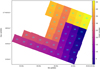 |
Fig. 13. MUSE-Wide field mapping. It returns a preferred field to use for any location located within the MUSE-Wide footprint based on the amount of exposures and the best observing conditions available for each coordinate. |
An image of the field map is shown in Fig. 13. One sees that fields with mediocre observing conditions, surrounded by less noisy fields such as candels-cdfs-29, have overall less space in the survey assigned to them. Each object of the photometric catalog got assigned to exactly one MUSE-Wide field based on this field mapping.
5.2. Optimal 3D spectral extraction
One further step was to extract 1D spectra of each individual source in our MUSE-Wide photometric catalog from the MUSE data cubes. To optimally extract flux-conserving spectra from 3D data, that is, spectra with the best possible signal-to-noise ratio, the spatial morphology and the wavelength dependent PSF described in Sect. 3.2.5 needed to be accounted for. Furthermore, good deblending of neighboring sources was essential to produce spectra representing the intrinsic spectra as accurately as possible. The spectra provided with the current data release and the classification of the brightest sources described in the next Section were extracted using version 2.0 of the dedicated tool “Three Dimensional Optimal Spectral Extraction” (TDOSE). TDOSE generalizes the concepts of Kamann et al. (2013) to extended non-PSF sources, that is, galaxies. TDOSE will be presented in Schmidt et al. (in prep.), and is publicly available from GitHub9. In the following we provide a short summary of the spectral extraction performed for this study but refer the reader to the above sources for further details on the tools and methods involved in the spectral extraction.
TDOSE uses PSF-convolved morphological models of photometric counterparts to simultaneously extract 1D spectra from the 3D MUSE cubes. This is done by solving a set of linear equations minimizing the difference between the object models convolved with the wavelength dependent MUSE PSF cube, scaled by some flux, and the observed flux in the final MUSE datacubes described in Sect. 3.2.4. To make this process fully analytic we used the Gaussian PSF estimation and described the galaxies by single multi-variate Gaussian models (Hogg & Lang 2013) or point sources. The latter models were used for objects with detected emission lines in the MUSE data (Sect. 4), but no or minimal photometric counterpart. The morphological models were generated using thecurve_fit optimizer of Scipy10 optimizer on the F814W CANDELS HST images. The F814W images were chosen due to their depth as well as the peak sensitivity wavelength and similarity in wavelength coverage of this filter (≈6880–9640 Å) with the MUSE wavelength coverage (4750–9350 Å).
Using single multi-variate Gaussians as source models, is obviously simplifying the often complicated morphology of galaxies. However, after convolving the HST-based models with the MUSE PSF, the loss of flux between the spectral extractions of single-component Gaussian model and a GALFIT (Peng et al. 2010) multiple-component Sérsic (1963) model is only ∼5% at the [O II] wavelength for a sample of ∼150 relatively bright (23 < F814W < 24) [O II] emitters in the MUSE-Wide CDF-S footprint. The exact amount of flux lost from using a simplified single-component model, of course depends on the intrinsic (HST) morphology of the sample studied.
Solving the set of linear equations simultaneously ensured optimal deblending of sources, when assembling the 1D spectra. TDOSE essentially assigns a fraction of the flux in each voxel of the MUSE datacube to objects contributing to these voxels according to their morphological PSF-convolved models. Solving the system of equations provided wavelength dependent flux scalings for each individual source (the sum of the factional flux scalings for all voxels) in the field-of-view of the MUSE datacubes. These χ2 minimizing flux-scalings were the 1D spectra used for object classification and are available on the data release webpage11 (see Appendix A).
The main assumption of the spectra extracted as part of this study, is that the light distribution is a multivariate Gaussian and follows the F814W continuum light distribution convolved with the Gaussian MUSE PSF at each wavelength of the MUSE datacubes. Given that most galaxies are known to follow non-Gaussian light distributions, for example, Sérsic (1963) profiles, or have multiple components and distinct features that might very well vary with wavelength, these assumptions are be somewhat restrictive and may depend the scientific applications of the spectra, but are only expected to results in flux-losses on the few-percent level, as described above. More fundamental, features that do not intrinsically follow the light-distribution of the continuum are expected to be biased in the TDOSE spectra.. In particular, as Lyα emission is known to be more extended than the continuum emission (Wisotzki et al. 2016; Leclercq et al. 2017), the TDOSE spectra are unsuitable for estimating total Lyα fluxes for the brightest LAEs in the MUSE-Wide sample. The same holds for the study of any other spectral features that do not, to a fair approximation, follow the distribution of the continuum light. This presumably includes all nebular emission lines, which often do not trace the spatial distribution of the stars that make up the continuum light modeled. Hence, the TDOSE spectra are “optimal” for the continuum sources, but are not necessarily so for wavelengths with emission lines.
However, for the public data release and for the classification of the brightest photometrically selected objects in MUSE-Wide based on their spectral features, the Gaussian assumptions are sufficiently detailed. We furthermore chose to use these simplifying assumptions, as they made the spectral extraction process fully analytic and provided a homogeneous sample of spectra for all objects in the data release, irrespective of object type, magnitude, size or redshift.
5.3. Identification of galaxies brighter than 24th magnitude
Of the 9205 photometrically selected objects, 772 have a F775W magnitude brighter than 24. We inspect the objects in this subset of the photometric catalog further to identify them spectroscopically. Even though we use MUSE spectra to classify this bright subset of the photometric catalog, we do not create separate MUSE IDs for the objects in this catalog, but keep the CANDELS ID for our classification. Since the photometric catalog links to the emission-line objects, we can discard objects, that have already assigned a redshift. 499 (64%) already were identified via their emission lines, we adopt the identification gleaned from the emission lines, leaving us to inspect 273 objects using the optimally extracted 1D TDOSE spectra. These non-emission line sources were primarily identified through their absorption features.
Similar to the MUSE-Deep approach (Inami et al. 2017), we used a modified version of the redshift fitting software MARZ (Hinton et al. 2016). MARZ determines redshifts based on a version of the AUTOZ cross-correlation algorithm (Baldry et al. 2014). We employed the redshift templates also used for MUSE-Deep. The cross-correlation was done with our TDOSE spectra by a team of investigators (L.W., K.B.S., D.K. and T.U.) first individually and later consolidated by agreeing on a template and a confidence number. Also here the confidence levels are somewhat subjective, but we tried to anchor it to the same rate as for the emission line sources, thus expecting less than 1%, 10% and 50% false identifications for confidence 3, confidence 2 and confidence 1 objects, respectively. We were able to identify 98% of the 772 objects with only 15 objects (2%) remaining unidentified. We release this identification subcatalog on the photometric catalog page of our data release page (see Appendix A.2).
Figure 14 shows the redshift distribution for the 757 identified objects brighter than 24th magnitude (772 objects – 15 non-identifications). Since this is a magnitude-limited sample, it is expected that the redshift distribution skews toward low redshift objects. Nevertheless we are able to identify some objects in the “redshift-desert” via their Mg II, Fe II and Al III absorption features. Our imposed 24th magnitude limit is clearly a conservative choice that ensures high success rate. Probably there are several objects fainter than 24th magnitude that are not in the emission line catalog, but that could be nonetheless be identified spectroscopically either through faint or broad emission lines not captured by LSDCat or through absorption lines associated with strong SED features (e.g., Ca H+K absorption with the 4000 Å jump). This is beyond the scope of this paper.
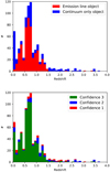 |
Fig. 14. Redshift identification of photometrically selected objects brighter than 24th magnitude. Shown are stacked histograms of the redshift distribution. Top panel: identification by type of object (emission-line object or continuum only object), lower panel: distribution of the confidence levels of the identification. |
The photometric catalog and the identification catalog for objects brighter than 24th magnitude are stored in the MUSE-Wide webpage (see Appendix A). The description of each field is given in the “Database” tab (see Appendix A.4). We have tried to keep the columns as simple and self-explanatory as possible providing only a coordinate, a few HST magnitudes and a possible association to the emission-line catalog for each object. The identification catalog only has two additional columns, one for the redshift, one for the confidence level of the identification.
6. Conclusions and outlook
We have presented the first data release of the MUSE-Wide survey, a blind 3D survey targeting well-known and studied deep fields with extensive multiwavelength data, such as the GOODS-S/CDFS and CANDELS-COSMOS areas. DR1 encompasses 39.5 arcmin2 over 44 MUSE fields in the GOODS-S/CDFS observed at a depth of one hour. It represents the wide, “shallow” component to the MUSE-Deep survey carried out in the HUDF (Bacon et al. 2017).
The main scientific contributions in this data release (and of deep blind 3D MUSE surveys in general) are the detection of emission line sources in the datacubes and the optimal extraction of 1D spectra based on the prior HST photometric information. Analysis of the spectra of these emission line objects and bright photometric objects yielded 1859 spectroscopic redshift identifications (1602 emission line objects + 257 continuum only objects), with 1597 of those being of high confidence (confidence ≥ 2). Even with only one hour integration times, this represents an unprecedented density of spectroscopic redshifts gathered in extragalactic surveys, surpassing even the deepest spectroscopic surveys by an order of magnitude (e.g., LBG-z3 – Steidel et al. 2003, FSF – Noll et al. 2004, VUDS – Le Fèvre et al. 2015, VANDELS – Pentericci et al. 2018).
Similar to Fig. 18 in Inami et al. (2017) of the MUSE-Deep catalog, in Fig. 15 we show the F775W magnitude over redshift of our high confidence sources. The black circles denote the sources with previous spectroscopic redshift identifications. From this Figure it is clear that MUSE-Wide opens up a new window at high redshift based on the detection of the Lyα line at z > 2.9. Naturally, there are some differences between the typical MUSE-Deep and MUSE-Wide identifications, since the MUSE-Deep data extends well over a magnitude deeper to analyze continuum spectra. We see this especially pronounced in the “redshift-desert” at 1.5 < z < 2.9, where MUSE-Deep is able to identify a number of objects based on their C III] emission or the absorption features seen in that range. MUSE-Deep offers an excellent opportunity to study large number of LAEs, the densities ever increasing at the faintest magnitudes. However, MUSE-Wide covers the LAEs with relatively bright UV counterparts, which offers the opportunity to study their stellar content with upcoming instruments, such as the James Webb Space Telescope (JWST). Another area where MUSE-Wide can probe new ground is in the identification of z < 1.5 emission-line dwarf field galaxies with magnitudes >24. Those sources are not typically targeted in redshifts surveys, either because they are too faint or because they have (correct) low photo-z values. MUSE-Deep can also easily find and identify them, however the density of these systems does not increase as rapidly with magnitude as for the LAEs; the spatial density seems to be better suited for a survey such as MUSE-Wide, with the bulk of the population having magnitudes magF775W = 24−27.
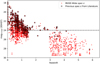 |
Fig. 15. F775W HST magnitude of both photometrically and emission-line selected high confidence sources (1597 objects with confidence ≥ 2) as a function of redshift. The red dots and arrows (upper magnitude limits) represent the MUSE spectroscopically determined redshifts, while the open black circles denote previous spectroscopic redshifts of those sources from the literature. The large amount of redshift identifications, especially at high redshift highlight the capabilities of MUSE-Wide as an incredibly effective redshift survey. |
Of course, a 3D survey such as MUSE-Wide can act as more than a simple redshift identification survey. The multiplexing capabilities of MUSE let us further characterize the identified sources, such as metallicity gradients at low redshift (Carton et al. 2018) or Lyα-halos at high redshift (Saust et al., in prep.).
A future and final data release will roughly double the current DR1 in size covering all 91+9 MUSE-Wide fields, including the 23 fields in the CANDELS-COSMOS region. We plan on improving the data reduction using learned insights and new software tools that were released since we froze our reduction pipeline early in the survey. The insights from the first 44 fields already predict that we will succeed reaching our goal of finding more than 1000 LAEs over the MUSE-Wide survey area.
When we refer to slices we mean the portion of light that is redirected by the MUSE image slicer and put through the pseudo-slits onto the CCD for each IFU. See Fig. 10 of the MUSE User Manual (version 8, http://www.eso.org/sci/facilities/paranal/instruments/muse/doc/ESO-261650_MUSE_User_Manual_8.pdf) for a reference of the slice positions on the CCD.
Tests on observations of Globular Clusters with MUSE show little discrepancy from the Moffat function accross the entire field of view (e.g., Husser et al. 2016).
This difference in the effective noise scale can be explained by the fact that the “old” recipe as used in H17 did not correct for the spectral resampling; this amounts to a factor 1.25 in the noise level, for standard MUSE settings.
http://ascl.net/1703.011, see Appendix A of H17 for a description of the functionality.
Using PIMMS: http://cxc.harvard.edu/toolkit/pimms.jsp and an unabsorbed power law model at redshift z = 4.0 with Galactic NH = 8.8 × 1019 cm−2. We employed the Chandra Cycle 10 ACIS-I filter for the countrate to flux conversion.
Acknowledgments
The authors give thanks to the staff at ESO for extensive support during the visitor-mode campaigns at Paranal Observatory. We thank the eScience group at AIP for help with the functionality of the MUSE-Wide data release webpage and in particular Ole Streicher for the development of the cut-out tool. We thank Nicolas Bouché for helpful comments that improved the manuscript. T.U., L.W., J.K., K.B.S., E.C.H, R.S., C.D. and J.C. acknowledge funding by the Competitive Fund of the Leibniz Association through grants SAW-2013-AIP-4 and SAW-2015-AIP-2. R.B. acknowledges support from the ERC advanced grant 339659-MUSICOS and the FOGHAR Project with ANR Grant ANR-13-BS05-0010. P.M.W. acknowledges support through BMBF Verbundforschung (project MUSE-AO, grant 05A14BAC). This work has made use of the Chandra Deep Field South Dataset, Dataset Identifier: ADS/Sa.CXO#Contrib/ChandraDeepFieldS This work has made use of observations taken by the CANDELS Multi-Cycle Treasury Program with the NASA/ESA HST, which is operated by the Association of Universities for Research in Astronomy, Inc., under NASA contract NAS5-26555. Based on data obtained with the European Southern Observatory Very Large Telescope, Paranal, Chile, under Large Program 185.A-0791, and made available by the VUDS team at the CESAM data center, Laboratoire d’Astrophysique de Marseille, France. This work has made use of observations taken by the 3D-HST Treasury Program (GO 12177 and 12328) with the NASA/ESA HST, which is operated by the Association of Universities for Research in Astronomy, Inc., under NASA contract NAS5-26555. This research made use of Astropy, a community-developed core Python package for Astronomy (Astropy Collaboration 2013).
References
- Ao, Y., Matsuda, Y., Beelen, A., et al. 2015, A&A, 581, A132 [NASA ADS] [CrossRef] [EDP Sciences] [Google Scholar]
- Astropy Collaboration (Robitaille, T. P., et al.) 2013, A&A, 558, A33 [NASA ADS] [CrossRef] [EDP Sciences] [Google Scholar]
- Atek, H., Malkan, M., McCarthy, P., et al. 2010, ApJ, 723, 104 [NASA ADS] [CrossRef] [Google Scholar]
- Bacon, R., Vernet, J., Borisova, E., et al. 2014, The Messenger, 157, 13 [NASA ADS] [Google Scholar]
- Bacon, R., Brinchmann, J., Richard, J., et al. 2015, A&A, 575, A75 [NASA ADS] [CrossRef] [EDP Sciences] [Google Scholar]
- Bacon, R., Conseil, S., Mary, D., et al. 2017, A&A, 608, A1 [NASA ADS] [CrossRef] [EDP Sciences] [Google Scholar]
- Baldry, I. K., Alpaslan, M., Bauer, A. E., et al. 2014, MNRAS, 441, 2440 [NASA ADS] [CrossRef] [Google Scholar]
- Baldwin, J. A., Phillips, M. M., & Terlevich, R. 1981, PASP, 93, 5 [NASA ADS] [CrossRef] [EDP Sciences] [Google Scholar]
- Balestra, I., Mainieri, V., Popesso, P., et al. 2010, A&A, 512, A12 [NASA ADS] [CrossRef] [EDP Sciences] [Google Scholar]
- Barro, G., Faber, S. M., Pérez-González, P. G., et al. 2013, ApJ, 765, 104 [NASA ADS] [CrossRef] [Google Scholar]
- Beckwith, S. V. W., Stiavelli, M., Koekemoer, A. M., et al. 2006, AJ, 132, 1729 [NASA ADS] [CrossRef] [Google Scholar]
- Behroozi, P. S., Wechsler, R. H., & Conroy, C. 2013, ApJ, 770, 57 [NASA ADS] [CrossRef] [Google Scholar]
- Bell, E. F., van der Wel, A., Papovich, C., et al. 2012, ApJ, 753, 167 [NASA ADS] [CrossRef] [Google Scholar]
- Bouwens, R. J., Illingworth, G. D., Oesch, P. A., et al. 2011, ApJ, 737, 90 [NASA ADS] [CrossRef] [Google Scholar]
- Bower, R. G., Morris, S. L., Bacon, R., et al. 2004, MNRAS, 351, 63 [NASA ADS] [CrossRef] [Google Scholar]
- Brammer, G. B., van Dokkum, P. G., & Coppi, P. 2008, ApJ, 686, 1503 [NASA ADS] [CrossRef] [Google Scholar]
- Brammer, G. B., van Dokkum, P. G., Franx, M., et al. 2012, ApJS, 200, 13 [Google Scholar]
- Brinchmann, J., Charlot, S., White, S. D. M., et al. 2004, MNRAS, 351, 1151 [NASA ADS] [CrossRef] [Google Scholar]
- Brinchmann, J., Inami, H., Bacon, R., et al. 2017, A&A, 608, A3 [NASA ADS] [CrossRef] [EDP Sciences] [Google Scholar]
- Bruzual, G., & Charlot, S. 2003, MNRAS, 344, 1000 [NASA ADS] [CrossRef] [Google Scholar]
- Calzetti, D., Armus, L., Bohlin, R. C., et al. 2000, ApJ, 533, 682 [NASA ADS] [CrossRef] [Google Scholar]
- Cardamone, C., Schawinski, K., Sarzi, M., et al. 2009, MNRAS, 399, 1191 [NASA ADS] [CrossRef] [Google Scholar]
- Carton, D., Brinchmann, J., Contini, T., et al. 2018, MNRAS, 478, 4293 [NASA ADS] [CrossRef] [Google Scholar]
- Caruana, J., Wisotzki, L., Herenz, E. C., et al. 2018, MNRAS, 473, 30 [NASA ADS] [CrossRef] [Google Scholar]
- Cassata, P., Tasca, L. A. M., Le Fèvre, O., et al. 2015, A&A, 573, A24 [NASA ADS] [CrossRef] [EDP Sciences] [Google Scholar]
- Chabrier, G. 2003, PASP, 115, 763 [NASA ADS] [CrossRef] [Google Scholar]
- Civano, F., Marchesi, S., Comastri, A., et al. 2016, ApJ, 819, 62 [NASA ADS] [CrossRef] [Google Scholar]
- Conseil, S., Bacon, R., Piqueras, L., & Shepherd, M. 2016, ArXiv e-prints [arXiv:1612.05308] [Google Scholar]
- Contini, T., Epinat, B., Bouché, N., et al. 2016, A&A, 591, A49 [NASA ADS] [CrossRef] [EDP Sciences] [Google Scholar]
- Dahlen, T., Mobasher, B., Faber, S. M., et al. 2013, ApJ, 775, 93 [Google Scholar]
- Davies, L. J. M., Robotham, A. S. G., Driver, S. P., et al. 2018, MNRAS, 480, 768 [NASA ADS] [CrossRef] [Google Scholar]
- Dawson, S., Rhoads, J. E., Malhotra, S., et al. 2004, ApJ, 617, 707 [NASA ADS] [CrossRef] [Google Scholar]
- Diener, C., Wisotzki, L., Schmidt, K. B., et al. 2017, MNRAS, 471, 3186 [NASA ADS] [CrossRef] [Google Scholar]
- Dijkstra, M., Gronke, M., & Venkatesan, A. 2016, ApJ, 828, 71 [NASA ADS] [CrossRef] [Google Scholar]
- Drake, A. B., Guiderdoni, B., Blaizot, J., et al. 2017, MNRAS, 471, 267 [NASA ADS] [CrossRef] [Google Scholar]
- Dressel, L. 2018, Wide Field Camera 3 Instrument Handbook, Version, 10 [Google Scholar]
- Elbaz, D., Dickinson, M., Hwang, H. S., et al. 2011, A&A, 533, A119 [NASA ADS] [CrossRef] [EDP Sciences] [Google Scholar]
- Erb, D. K., Bogosavljević, M., & Steidel, C. C. 2011, ApJ, 740, L31 [NASA ADS] [CrossRef] [Google Scholar]
- Gawiser, E., Francke, H., Lai, K., et al. 2007, ApJ, 671, 278 [NASA ADS] [CrossRef] [Google Scholar]
- Giacconi, R., Rosati, P., Tozzi, P., et al. 2001, ApJ, 551, 624 [NASA ADS] [CrossRef] [Google Scholar]
- Giallongo, E., Grazian, A., Fiore, F., et al. 2015, A&A, 578, A83 [NASA ADS] [CrossRef] [EDP Sciences] [Google Scholar]
- Giavalisco, M., Ferguson, H. C., Koekemoer, A. M., et al. 2004, ApJ, 600, L93 [NASA ADS] [CrossRef] [Google Scholar]
- Grogin, N. A., Kocevski, D. D., Faber, S. M., et al. 2011, ApJS, 197, 35 [NASA ADS] [CrossRef] [Google Scholar]
- Gronke, M. 2017, A&A, 608, A139 [Google Scholar]
- Gronwall, C., Ciardullo, R., Hickey, T., et al. 2007, ApJ, 667, 79 [NASA ADS] [CrossRef] [Google Scholar]
- Guérou, A., Krajnović, D., Epinat, B., et al. 2017, A&A, 608, A5 [NASA ADS] [CrossRef] [EDP Sciences] [Google Scholar]
- Guo, Y., Ferguson, H. C., Giavalisco, M., et al. 2013, ApJS, 207, 24 [NASA ADS] [CrossRef] [Google Scholar]
- Hagen, A., Zeimann, G. R., Behrens, C., et al. 2016, ApJ, 817, 79 [NASA ADS] [CrossRef] [EDP Sciences] [Google Scholar]
- Hashimoto, T., Ouchi, M., Shimasaku, K., et al. 2017a, MNRAS, 465, 1543 [NASA ADS] [CrossRef] [Google Scholar]
- Hashimoto, T., Garel, T., Guiderdoni, B., et al. 2017b, A&A, 608, A10 [NASA ADS] [CrossRef] [EDP Sciences] [Google Scholar]
- Herenz, E. C., & Wisotzki, L. 2017, A&A, 602, A111 [NASA ADS] [CrossRef] [EDP Sciences] [Google Scholar]
- Herenz, E. C., Urrutia, T., Wisotzki, L., et al. 2017, A&A, 606, A12 [NASA ADS] [CrossRef] [EDP Sciences] [Google Scholar]
- Herenz, E. C., Wisotzki, L., Saust, R., et al. 2019, A&A, 621, A107 [NASA ADS] [CrossRef] [EDP Sciences] [Google Scholar]
- Hildebrandt, H., Erben, T., Dietrich, J. P., et al. 2006, A&A, 452, 1121 [NASA ADS] [CrossRef] [EDP Sciences] [Google Scholar]
- Hinton, S. R., Davis, T. M., Lidman, C., Glazebrook, K., & Lewis, G. F. 2016, Astron. Comput., 15, 61 [NASA ADS] [CrossRef] [Google Scholar]
- Hodge, J. A., Karim, A., Smail, I., et al. 2013, ApJ, 768, 91 [NASA ADS] [CrossRef] [Google Scholar]
- Hogg, D. W., & Lang, D. 2013, PASP, 125, 719 [NASA ADS] [CrossRef] [Google Scholar]
- Hornschemeier, A. E., Brandt, W. N., Garmire, G. P., et al. 2001, ApJ, 554, 742 [NASA ADS] [CrossRef] [Google Scholar]
- Hsu, L.-T., Salvato, M., Nandra, K., et al. 2014, ApJ, 796, 60 [NASA ADS] [CrossRef] [Google Scholar]
- Hu, E. M., & McMahon, R. G. 1996, Nature, 382, 231 [NASA ADS] [CrossRef] [Google Scholar]
- Husser, T.-O., Kamann, S., Dreizler, S., et al. 2016, A&A, 588, A148 [NASA ADS] [CrossRef] [EDP Sciences] [Google Scholar]
- Inami, H., Bacon, R., Brinchmann, J., et al. 2017, A&A, 608, A2 [NASA ADS] [CrossRef] [EDP Sciences] [Google Scholar]
- Izotov, Y. I., Schaerer, D., Thuan, T. X., et al. 2016, MNRAS, 461, 3683 [NASA ADS] [CrossRef] [Google Scholar]
- Izotov, Y. I., Schaerer, D., Worseck, G., et al. 2018, MNRAS, 474, 4514 [NASA ADS] [CrossRef] [Google Scholar]
- Juneau, S., Dickinson, M., Alexander, D. M., & Salim, S. 2011, ApJ, 736, 104 [NASA ADS] [CrossRef] [Google Scholar]
- Kamann, S., Wisotzki, L., & Roth, M. M. 2013, A&A, 549, A71 [NASA ADS] [CrossRef] [EDP Sciences] [Google Scholar]
- Karim, A., Schinnerer, E., Martínez-Sansigre, A., et al. 2011, ApJ, 730, 61 [NASA ADS] [CrossRef] [Google Scholar]
- Kashikawa, N., Nagao, T., Toshikawa, J., et al. 2012, ApJ, 761, 85 [NASA ADS] [CrossRef] [Google Scholar]
- Kellermann, K. I., Fomalont, E. B., Mainieri, V., et al. 2008, ApJS, 179, 71 [NASA ADS] [CrossRef] [Google Scholar]
- Kerutt, J. 2017, Astrophysics Source Code Library [record ascl:1703.011] [Google Scholar]
- Koekemoer, A. M., Faber, S. M., Ferguson, H. C., et al. 2011, ApJS, 197, 36 [NASA ADS] [CrossRef] [Google Scholar]
- Kriek, M., van Dokkum, P. G., Labbé, I., et al. 2009, ApJ, 700, 221 [NASA ADS] [CrossRef] [Google Scholar]
- Kudritzki, R.-P., Méndez, R. H., Feldmeier, J. J., et al. 2000, ApJ, 536, 19 [NASA ADS] [CrossRef] [Google Scholar]
- Laigle, C., McCracken, H. J., Ilbert, O., et al. 2016, ApJS, 224, 24 [NASA ADS] [CrossRef] [Google Scholar]
- Leclercq, F., Bacon, R., Wisotzki, L., et al. 2017, A&A, 608, A8 [NASA ADS] [CrossRef] [EDP Sciences] [Google Scholar]
- Le Fèvre, O., Vettolani, G., Garilli, B., et al. 2005, A&A, 439, 845 [NASA ADS] [CrossRef] [EDP Sciences] [Google Scholar]
- Le Fèvre, O., Tasca, L. A. M., Cassata, P., et al. 2015, A&A, 576, A79 [NASA ADS] [CrossRef] [EDP Sciences] [Google Scholar]
- Lilly, S. J., Le Fèvre, O., Renzini, A., et al. 2007, ApJS, 172, 70 [NASA ADS] [CrossRef] [Google Scholar]
- Luo, B., Brandt, W. N., Alexander, D. M., et al. 2014, ApJ, 794, 70 [NASA ADS] [CrossRef] [Google Scholar]
- Luo, B., Brandt, W. N., Xue, Y. Q., et al. 2017, ApJS, 228, 2 [Google Scholar]
- Mainieri, V., Rigopoulou, D., Lehmann, I., et al. 2005, MNRAS, 356, 1571 [NASA ADS] [CrossRef] [Google Scholar]
- Marchi, F., Pentericci, L., Guaita, L., et al. 2017, A&A, 601, A73 [NASA ADS] [CrossRef] [EDP Sciences] [Google Scholar]
- Maseda, M. V., van der Wel, A., Rix, H.-W., et al. 2018a, ApJ, 854, 29 [NASA ADS] [CrossRef] [Google Scholar]
- Maseda, M. V., Bacon, R., Franx, M., et al. 2018b, ApJ, 865, L1 [NASA ADS] [CrossRef] [Google Scholar]
- Matsuda, Y., Yamada, T., Hayashino, T., et al. 2011, MNRAS, 410, L13 [NASA ADS] [CrossRef] [Google Scholar]
- Miller, N. A., Fomalont, E. B., Kellermann, K. I., et al. 2008, ApJS, 179, 114 [NASA ADS] [CrossRef] [Google Scholar]
- Miyaji, T., Griffiths, R. E., & C-COSMOS Team. 2008, AAS/High Energy Astrophys. Div. #10, 10, 4.01 [Google Scholar]
- Moffat, A. F. J. 1969, A&A, 3, 455 [NASA ADS] [Google Scholar]
- Momcheva, I. G., Brammer, G. B., van Dokkum, P. G., et al. 2016, ApJS, 225, 27 [NASA ADS] [CrossRef] [Google Scholar]
- Mullaney, J. R., Del-Moro, A., Aird, J., et al. 2015, ApJ, 808, 184 [NASA ADS] [CrossRef] [Google Scholar]
- Nanayakkara, T., Glazebrook, K., Kacprzak, G. G., et al. 2016, ApJ, 828, 21 [NASA ADS] [CrossRef] [Google Scholar]
- Nilsson, K. K., Fynbo, J. P. U., Møller, P., Sommer-Larsen, J., & Ledoux, C. 2006, A&A, 452, L23 [NASA ADS] [CrossRef] [EDP Sciences] [Google Scholar]
- Noeske, K. G., Weiner, B. J., Faber, S. M., et al. 2007, ApJ, 660, L43 [Google Scholar]
- Noll, S., Mehlert, D., Appenzeller, I., et al. 2004, A&A, 418, 885 [NASA ADS] [CrossRef] [EDP Sciences] [Google Scholar]
- Norman, C., Hasinger, G., Giacconi, R., et al. 2002, ApJ, 571, 218 [NASA ADS] [CrossRef] [Google Scholar]
- Ouchi, M., Shimasaku, K., Furusawa, H., et al. 2003, ApJ, 582, 60 [NASA ADS] [CrossRef] [Google Scholar]
- Ouchi, M., Harikane, Y., Shibuya, T., et al. 2018, PASJ, 70, S13 [NASA ADS] [CrossRef] [Google Scholar]
- Oliver, S. J., Bock, J., Altieri, B., et al. 2012, MNRAS, 424, 1614 [NASA ADS] [CrossRef] [EDP Sciences] [Google Scholar]
- Oyarzún, G. A., Blanc, G. A., González, V., et al. 2016, ApJ, 821, L14 [NASA ADS] [CrossRef] [Google Scholar]
- Paalvast, M., Verhamme, A., Straka, L. A., et al. 2018, A&A, 618, A40 [NASA ADS] [CrossRef] [EDP Sciences] [Google Scholar]
- Partridge, R. B., & Peebles, P. J. E. 1967, ApJ, 147, 868 [NASA ADS] [CrossRef] [Google Scholar]
- Peng, C. Y., Ho, L. C., Impey, C. D., & Rix, H.-W. 2010, AJ, 139, 2097 [NASA ADS] [CrossRef] [Google Scholar]
- Pentericci, L., McLure, R. J., Garilli, B., et al. 2018, A&A, 616, A174 [NASA ADS] [CrossRef] [EDP Sciences] [Google Scholar]
- Prescott, M. K. M., Momcheva, I., Brammer, G. B., Fynbo, J. P. U., & Møller, P. 2015, ApJ, 802, 32 [NASA ADS] [CrossRef] [Google Scholar]
- Raiter, A., Schaerer, D., & Fosbury, R. A. E. 2010, A&A, 523, A64 [NASA ADS] [CrossRef] [EDP Sciences] [Google Scholar]
- Rhoads, J. E., Malhotra, S., Dey, A., et al. 2000, ApJ, 545, L85 [NASA ADS] [CrossRef] [Google Scholar]
- Ryabchikova, T., Piskunov, N., Kurucz, R. L., et al. 2015, Phys. Scr, 90, 054005 [NASA ADS] [CrossRef] [Google Scholar]
- Schinnerer, E., Sargent, M. T., Bondi, M., et al. 2010, ApJS, 188, 384 [NASA ADS] [CrossRef] [Google Scholar]
- Scoville, N., Aussel, H., Brusa, M., et al. 2007, ApJS, 172, 1 [NASA ADS] [CrossRef] [Google Scholar]
- Sérsic, J. L. 1963, Boletin de la Asociacion Argentina de Astronomia La Plata Argentina, 6, 41 [Google Scholar]
- Shibuya, T., Kashikawa, N., Ota, K., et al. 2012, ApJ, 752, 114 [Google Scholar]
- Shibuya, T., Ouchi, M., Nakajima, K., et al. 2014, ApJ, 788, 74 [NASA ADS] [CrossRef] [Google Scholar]
- Skelton, R. E., Whitaker, K. E., Momcheva, I. G., et al. 2014, ApJS, 214, 24 [Google Scholar]
- Sobral, D., Matthee, J., Darvish, B., et al. 2015, ApJ, 808, 139 [NASA ADS] [CrossRef] [Google Scholar]
- Sobral, D., Matthee, J., Best, P., et al. 2017, MNRAS, 466, 1242 [NASA ADS] [CrossRef] [Google Scholar]
- Soto, K. T., Lilly, S. J., Bacon, R., Richard, J., & Conseil, S. 2016, MNRAS, 458, 3210 [NASA ADS] [CrossRef] [Google Scholar]
- Speagle, J. S., Steinhardt, C. L., Capak, P. L., & Silverman, J. D. 2014, ApJS, 214, 15 [NASA ADS] [CrossRef] [Google Scholar]
- Stark, D. P., Ellis, R. S., Chiu, K., Ouchi, M., & Bunker, A. 2010, MNRAS, 408, 1628 [NASA ADS] [CrossRef] [Google Scholar]
- Stark, D. P., Schenker, M. A., Ellis, R., et al. 2013, ApJ, 763, 129 [NASA ADS] [CrossRef] [Google Scholar]
- Stark, D. P., Richard, J., Siana, B., et al. 2014, MNRAS, 445, 3200 [NASA ADS] [CrossRef] [Google Scholar]
- Steidel, C. C., Adelberger, K. L., Shapley, A. E., et al. 2000, ApJ, 532, 170 [NASA ADS] [CrossRef] [Google Scholar]
- Steidel, C. C., Adelberger, K. L., Shapley, A. E., et al. 2003, ApJ, 592, 728 [NASA ADS] [CrossRef] [Google Scholar]
- Streicher, O., Weilbacher, P. M., Bacon, R., & Jarno, A. 2011, in Astronomical Data Analysis Software and Systems XX, eds. I. N. Evans, A. Accomazzi, D. J. Mink, & A. H. Rots, ASP Conf. Ser., 442, 257 [NASA ADS] [Google Scholar]
- Szokoly, G. P., Bergeron, J., Hasinger, G., et al. 2004, ApJS, 155, 271 [NASA ADS] [CrossRef] [Google Scholar]
- Taniguchi, Y., Scoville, N., Murayama, T., et al. 2007, ApJS, 172, 9 [NASA ADS] [CrossRef] [Google Scholar]
- Tasca, L. A. M., Le Fèvre, O., Ribeiro, B., et al. 2017, A&A, 600, A110 [NASA ADS] [CrossRef] [EDP Sciences] [Google Scholar]
- Tokovinin, A. 2002, PASP, 114, 1156 [NASA ADS] [CrossRef] [Google Scholar]
- Trebitsch, M., Verhamme, A., Blaizot, J., & Rosdahl, J. 2016, A&A, 593, A122 [Google Scholar]
- Treister, E., Schawinski, K., Volonteri, M., & Natarajan, P. 2013, ApJ, 778, 130 [NASA ADS] [CrossRef] [Google Scholar]
- Vanzella, E., Cristiani, S., Dickinson, M., et al. 2008, A&A, 478, 83 [NASA ADS] [CrossRef] [EDP Sciences] [Google Scholar]
- Vito, F., Gilli, R., Vignali, C., et al. 2016, MNRAS, 463, 348 [NASA ADS] [CrossRef] [Google Scholar]
- Weigel, A. K., Schawinski, K., Treister, E., et al. 2015, MNRAS, 448, 3167 [NASA ADS] [CrossRef] [Google Scholar]
- Weijmans, A.-M., Bower, R. G., Geach, J. E., et al. 2010, MNRAS, 402, 2245 [NASA ADS] [CrossRef] [Google Scholar]
- Weilbacher, P. M., Streicher, O., & Urrutia, T. 2014, in Astronomical Data Analysis Software and Systems XXIII, eds. N. Manset, & P. Forshay, ASP Conf. Ser., 485, 451 [NASA ADS] [Google Scholar]
- Wilkins, S. M., Coulton, W., Caruana, J., et al. 2013, MNRAS, 435, 2885 [NASA ADS] [CrossRef] [Google Scholar]
- Williams, R. E., Blacker, B., Dickinson, M., et al. 1996, AJ, 112, 1335 [NASA ADS] [CrossRef] [Google Scholar]
- Wisotzki, L., Bacon, R., Blaizot, J., et al. 2016, A&A, 587, A98 [NASA ADS] [CrossRef] [EDP Sciences] [Google Scholar]
- Wuyts, S., Labbé, I., Förster Schreiber, N. M., et al. 2008, ApJ, 682, 985 [NASA ADS] [CrossRef] [Google Scholar]
- Wuyts, S., Förster Schreiber, N. M., van der Wel, A., et al. 2011, ApJ, 742, 96 [NASA ADS] [CrossRef] [Google Scholar]
- Xue, Y. Q., Luo, B., Brandt, W. N., et al. 2011, ApJS, 195, 10 [NASA ADS] [CrossRef] [Google Scholar]
- Yang, Y., Zabludoff, A., Jahnke, K., et al. 2011, ApJ, 735, 87 [NASA ADS] [CrossRef] [Google Scholar]
Appendix A: Data release webpage
We have described the first public data release from the MUSE-Wide survey, dubbed DR1. All data are available on the MUSE-Wide data release webpage12. The data release web page was created using the Open Source Daiquiri framework13. DR1 contains the cubes, spectra and catalogs for the first 44 fields in the candels-cdfs region. The page also functions as survey webpage providing news and notifications about the MUSE-Wide survey.
A screenshot of the landing page as of October 2018 is shown in Fig. A.1. Most of the data is accessible via tabs. Clicking on each tab opens up a new window, the contents of which are described in the subsections below. The login is optional for blog notification, commenting functionality and for storing SQL queries. Further data releases will also occur via this webpage. Tables within the webpage are registered with the Virtual Observatory, and each MUSE-Wide cube and MUSE-Wide object (either emission-line source or TDOSE extracted spectrum) has a citable DOI.
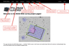 |
Fig. A.1. Screenshot of the MUSE-Wide data release landing page. The data is accessed throughout the various tabs described in this section. |
A.1. MUSE-Wide fields
The “Fields” page first lists links to our DR1 exposure map and the field mapping to assign a field number to each coordinate within the MUSE-Wide footprint. It then shows a table with five columns: the field name, linking to an individual field subpage, the RA/Dec of the center of the field, the datacube headers for each field and a link to download the corresponding datacube. We warn the user that each cube is about 5GB in size, which should be kept in mind when downloading MUSE-Wide cubes.
The individual field subpage on the top again provides links to the headers and to download the datacube, but more importantly to the quality control (QC) pages for each field. These QC pages show important numbers that characterize each field, such as the observing dates/conditions, the PSF estimation, the determined effective noise, the sky brightness, offset information and pseudo-broad-band MUSE images for different HST bands. The individual field pages lastly show a table of CANDELS/GUO photometric objects in that field on the basis of the field mapping. The table is searchable and sortable and shows the position, various magnitudes and possible link to an emission-line source. Clicking on the individual CANDELS/GUO ID opens up yet another subpage for that individual photometric object, which we describe below.
A.2. MUSE-Wide catalogs
Clicking on the “Catalogs” tab opens a drop-down menu in which one can select either the photometric or emission line catalog tables. The creation of these catalogs and their respective 1D spectra has been discussed in the respective sections in this paper (Sects. 4.1 and 5.2).
Clicking on the photometric catalog subtab opens up the “photometric catalog” subpage. At the top are the links to the complete 9205 object catalog and to the identification catalog of objects brighter than 24th magnitude (see Sect. 5.3). Below the links is a searchable and sortable table for all photometric catalog objects, along with clickable links to an individual object subpage, link to the corresponding field webpage (see previous section) and to a possible linked emission-line source subpage.
The individual object subpages first show an image of a smoothed spectrum (with a nine pixel or 11.25 Å Hanning window, also known as an inverse cosine bell14), a link to download a TDOSE-generated 1D spectrum and a link to download a cutout 6″ × 6″ minicube on the position of the object generated on-the-fly. Lastly the object subpage shows 6″ × 6″ postage stamps of GOODS-S and CANDELS HST images as well as a MUSE whitelight image centered on the objects position. At the center of the postage stamp is a red circle with a 1″ radius to help identify the center of the postage stamp.
Clicking on the emission line catalog subtab then opens the “Emission line catalog” subpage, which has the same layout as the photometric catalog page, only that at the top the linked catalogs are the main and emission line catalogs. The sortable and searchable table contains the information for emission lines, again including links to either emission-line objects subpages, the link to the field page and links to the associated CANDELS-GUO subpage. The layout for the emission-line object subpage is also very similar to the individual photometric object subpages with images of the spectrum, postages, links to the 1D spectrum and links to download a 6″ × 6″ minicube are all present in this subpage. There are links to both PSF-weighted and aperture 1D spectra centered on the LSDCat first moment position.
A.3. Minicube cutout tool
The “Cut-Out” subpage provides the user the opportunity to download a custom made 3D minicube on positions centered on the MUSE-Wide footprint. It will download only cube-data from one field according to the Field mapping described in Sect. 5.1 and includes all extensions of the MUSE-Wide data cube (flux, effective noise, exposure and whitelight). The minicube can have spatial sizes between 1″ and 20″ and may encompass either a portion or the whole wavelength range from 4750 to 9350 Å. The default is a 6″ × 6″ using the whole wavelength range. The default minicubes have file sizes of approximately 125MB.
A.4. SQL query page and database descriptors
The SQL query page allows the user to initiate more complicated search queries using the various catalogs and images of MUSE-Wide. It also allows cross-correlation to Simbad and VizieR. A simple SQL example on how to select the ten LAEs with the highest Lyα flux and their respective F775W HST magnitudes with MUSE-Wide DR1 is shown below:
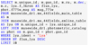
The “Database” subpage provides the formal description of all the data released in MUSE-Wide DR1. We opted to forgo a detailed description of the tables in this paper, since it can be found in this tab. It is possible to query for all entries presented within the various released tables, catalogs and metadata. For both the emission-line catalogs and the photometric catalogs a formal description each column and data format of each catalog and the metadata linking the catalogs and fields to each other can be found in this section.
All Tables
Counterpart percentages between the emission line sources to HST selected catalogs.
Catastrophic failures for objects with spectroscopic redshifts from the literature.
Table of matched X-ray objects with only photo-z values or disagreement between the redshifts.
All Figures
|
Fig. 1. Layout of the 91 fields observed for the MUSE-Wide survey in blue. Left: footprint in the Chandra Deep-Field South region overlaid on the V-Band image from the Garching-Bonn Deep Survey (GaBoDS; Hildebrandt et al. 2006). Shown in red are the approximate contours of the GOODS-S ACS and in yellow of the CANDELS-DEEP and HUDF09 parallels WFC3 regions. The magenta regions represent the nine MUSE-Deep intermediate depth mosaic of the HUDF. The current data release encompasses the fields enclosed by the thick black line. Right: footprint in the COSMOS region overlaid on the SUBARU-COSMOS i’-Band image (Taniguchi et al. 2007) available from IRSA (http://irsa.ipac.caltech.edu/Missions/cosmos.html). The red contours denote the southern tip of the deep HST exposures in the CANDELS-COSMOS region. |
| In the text | |
|
Fig. 2. Absolute RA/Dec offsets of the individual 15 min MUSE exposures to the CANDELS WFC3 160W coordinates (shaded in blue are the offset distributions). Most offsets are around 1″. |
| In the text | |
|
Fig. 3. Left: whitelight image of a single 15 minute exposure of a cube with only a few bright galaxies in the field (candels-cdfs-20), so that the contrast is enhanced. The dark regions in the slicer stack transitions immediately become visible. The regions in which the lowest 2% voxels are masked are marked by the green straight lines. Right: example of a collapsed, combined 4 × 900s exposure cube (candels-cdfs-01) showing the different exposure times at the edges due to the trapezoidal shape of the MUSE field of view. The square pattern shows the regions masked in the slicer stack transitions. |
| In the text | |
|
Fig. 4. Combined exposure maps of all 44 DR1 fields showing the coverage of the MUSE-Wide areas including the overlap regions which show up to 16 × 15 min exposures. |
| In the text | |
|
Fig. 5. Example of determined PSF slopes for the various methods on the field candels-cdfs-45: in the upper panel for the Gaussian p0 and p1 values and in the lower for the Moffat values. Methods (as described in text): P = direct fitting of stars, C = hybrid method of fitting stars and galaxies combined, F = Fast Fourier Transfrom. The final selected method is marked in bold letters. |
| In the text | |
|
Fig. 6. Left: distribution of number of emission-line objects as a function of S/N of the lead line for each of the three confidence levels we employ for classification. Objects at the S/N limit are dominated by confidence 1 objects and may include some spurious lines, while for objects with S/N above 10, we expect hardly any misclassifications. Right: redshift histogram of the emission line sources classified by their strongest line. The redshift desert, where there are no strong emission lines in the MUSE wavelength range between 1.5 < z < 2.9, is clearly visible. We are able to find 479 LAEs, reaching densities of almost 12 LAEs/arcmin2. |
| In the text | |
|
Fig. 7. Stack of normalized spectra of the emission line objects. They are stacked in y-direction with increasing redshifts, with a large jump between z∼1.5 and z∼2.9. First we normalized the spectra to the brightest emission line, then we smoothed with a 10 Å Gaussian and finally we smoothed the 2D image with a 2.8 pixel 2D circular Gaussian. |
| In the text | |
|
Fig. 8. Redshift comparison between MUSE and literature redshifts for our emission line selected galaxies. Red dots denote the compilation of redshifts from the literature gathered in Skelton et al. (2014). Magenta hexagons represent spectroscopic measurements from VUDS (Tasca et al. 2017). Green crosses represent grism spectroscopic redshifts from Momcheva et al. (2016), which were aided by the photometric redshifts from Skelton et al. (2014) denoted with blue crosses. The thin dashed lines show the regions outside of which a photometric redshift is determined as a catastrophic failure. |
| In the text | |
|
Fig. 9. Stellar mass histogram for emission-line objects with photometric counterparts, in red for high-redshift LAEs, in blue for lower redshift objects. We find a tail of low mass dwarf galaxies representing some of the lowest mass galaxies known at these redshifts. |
| In the text | |
|
Fig. 10. Photometric mass estimates fixed at the MUSE-Wide spectroscopic redshifts compared to the Skelton et al. (2014) photometric mass estimates based on photometric redshift estimates. The solid line represents the 1:1 mass equivalency, while the dashed lines show ±1 dex differences between the two stellar mass estimates. Marked with blue triangles are catastrophic redshift outliers, which will be the main cause of discrepancies. At low redshift there is good agreement between the stellar masses, while at high redshift the scatter between the masses is larger due to the large photometric errors associated with these faint galaxies. |
| In the text | |
|
Fig. 11. Null result of stacking X-ray images from the 4Ms CDFS data at LAE positions. The panels on the left refer to the soft band (0.3–2.0 keV), the ones on the right to the hard band (2.0–7.0 keV). Upper panels: stacked images, whichare 20″ × 20″ interpolated on a 0.5″ pixel size Chandra grid. Lower panels: statistics of the mean stack. |
| In the text | |
|
Fig. 12. CANDELS WFC3 6″ × 6″ cutout of the region centered on ALESS 10.1. CANDELS photometric objects from Guo et al. (2013) are marked in green, a MUSE-Wide emission galaxy with a 0.8″ radius in magenta, the X-ray source with its corresponding error radius in cyan and the ALESS source with an arbitrary 1.5″ radius in red. |
| In the text | |
|
Fig. 13. MUSE-Wide field mapping. It returns a preferred field to use for any location located within the MUSE-Wide footprint based on the amount of exposures and the best observing conditions available for each coordinate. |
| In the text | |
|
Fig. 14. Redshift identification of photometrically selected objects brighter than 24th magnitude. Shown are stacked histograms of the redshift distribution. Top panel: identification by type of object (emission-line object or continuum only object), lower panel: distribution of the confidence levels of the identification. |
| In the text | |
|
Fig. 15. F775W HST magnitude of both photometrically and emission-line selected high confidence sources (1597 objects with confidence ≥ 2) as a function of redshift. The red dots and arrows (upper magnitude limits) represent the MUSE spectroscopically determined redshifts, while the open black circles denote previous spectroscopic redshifts of those sources from the literature. The large amount of redshift identifications, especially at high redshift highlight the capabilities of MUSE-Wide as an incredibly effective redshift survey. |
| In the text | |
|
Fig. A.1. Screenshot of the MUSE-Wide data release landing page. The data is accessed throughout the various tabs described in this section. |
| In the text | |
Current usage metrics show cumulative count of Article Views (full-text article views including HTML views, PDF and ePub downloads, according to the available data) and Abstracts Views on Vision4Press platform.
Data correspond to usage on the plateform after 2015. The current usage metrics is available 48-96 hours after online publication and is updated daily on week days.
Initial download of the metrics may take a while.