| Issue |
A&A
Volume 677, September 2023
|
|
|---|---|---|
| Article Number | A138 | |
| Number of page(s) | 12 | |
| Section | Extragalactic astronomy | |
| DOI | https://doi.org/10.1051/0004-6361/202347026 | |
| Published online | 20 September 2023 | |
Identifying Lyα emitter candidates with Random Forest: Learning from galaxies in the CANDELS survey
1
INAF – Osservatorio Astronomico di Roma, via Frascati 33, 00078 Monteporzio Catone, Italy
e-mail: This email address is being protected from spambots. You need JavaScript enabled to view it.
2
Dipartimento di Fisica, Università di Roma Sapienza, Città Universitaria di Roma – Sapienza, Piazzale Aldo Moro 2, 00185 Roma, Italy
3
Dipartimento di Fisica, Università di Roma Tor Vergata, Via della Ricerca Scientifica 1, 00133 Roma, Italy
4
The Cosmic Dawn Centre (DAWN), Niels Bohr Institute, University of Copenhagen, Lyngbyvej 2, 2100 Copenhagen, Denmark
5
Dipartimento di Fisica e Astronomia, Università di Padova, Vicolo dell’Osservatorio 3, 35122 Padova, Italy
6
INAF – Osservatorio Astronomico di Padova, Vicolo dell’Osservatorio 5, 35122 Padova, Italy
7
Space Telescope Science Institute, 3700 San Martin Drive, Baltimore, MD, 21218
USA
8
INAF – Osservatorio di Astrofisica e Scienza dello Spazio di Bologna, Via P. Gobetti 93/3, 40129 Bologna, Italy
9
Institute for Advanced Research, Nagoya University, Nagoya, 464-8601
Japan
10
Department of Physics, Graduate School of Science, Nagoya University, Nagoya, 464-8602
Japan
Received:
26
May
2023
Accepted:
20
July
2023
Abstract
The physical processes that make a galaxy a Lyman alpha emitter have been extensively studied over the past 25 yr. However, the correlations between physical and morphological properties of galaxies and the strength of the Lyα emission line are still highly debated. Here, we investigate the correlations between the rest-frame Lyα equivalent width and stellar mass, star formation rate, dust reddening, metallicity, age, half-light semi-major axis, Sérsic index, and projected axis ratio in a sample of 1578 galaxies in the redshift range of 2 ≤ z ≤ 7.9 from the GOODS-S, UDS, and COSMOS fields. From the large sample of Lyα emitters (LAEs) in the dataset, we find that LAEs are typically common main sequence (MS) star-forming galaxies that show a stellar mass ≤109 M⊙, star formation rate ≤ 100.5 M⊙ yr−1, E(B − V)≤0.2, and half-light semi-major axis ≤1 kpc. Building on these findings, we have developed a new method based on a random forest (RF) machine learning (ML) classifier to select galaxies with the highest probability of being Lyα emitters. When applied to a population in the redshift range z ∈ [2.5, 4.5], our classifier holds a (80 ± 2)% accuracy and (73 ± 4)% precision. At higher redshifts (z ∈ [4.5, 6]), we obtained an accuracy of 73% and precision of 80%. These results highlight the possibility of overcoming the current limitations in assembling large samples of LAEs by making informed predictions that can be used for planning future large-scale spectroscopic surveys.
Key words: galaxies: high-redshift / galaxies: star formation / galaxies: ISM / dark ages / reionization / first stars
© The Authors 2023
 Open Access article, published by EDP Sciences, under the terms of the Creative Commons Attribution License (https://creativecommons.org/licenses/by/4.0), which permits unrestricted use, distribution, and reproduction in any medium, provided the original work is properly cited.
This article is published in open access under the Subscribe to Open model. This email address is being protected from spambots. You need JavaScript enabled to view it. to support open access publication.
1. Introduction
The Lyα emission line is one of the brightest emission lines produced in star-forming galaxies, due to the abundance of hydrogen and because it is produced by a common atomic electron transition. At z > 2 and z > 7, the line shifts (respectively) to the optical and near-IR regime and, thus, it allows us to identity faint high-z objects very efficiently. Throughout 25 years of observations and discoveries (e.g., Steidel et al. 1996; Stiavelli et al. 2001; Ouchi et al. 2003; Hayashino et al. 2004; Pentericci et al. 2018; Saxena et al. 2023), Lyα has shifted the observational redshift frontier, shedding light on the Epoch of Reionization (EoR) at z > 6.
Traditionally, Lyα emitting galaxies are defined as Lyα emitters (LAEs) if they show a rest-frame Lyα equivalent width of EW0 ≥ 20 Å (for details, see Shibuya et al. 2019; Ouchi et al. 2020; Runnholm et al. 2020). Searches for LAEs are often conducted through the use of narrow band (NB) filters (with variable central λNB and width δNB limited to 100 Å–200 Å, see Cowie & Hu 1998; Ajiki et al. 2003; Gronwall et al. 2007; Grove et al. 2009) that pinpoint the emission line in a certain redshift range targeted, namely, z = (λNB ± δNB)/1216 @@@−1. In this case, the basic technique of finding LAE candidates involves comparing images taken through a narrow-band filter (which samples the flux from the emission line) with a broad-band one at close wavelengths (which samples the continuum emission). At increasingly high redshifts, the efficiency of this approach on ground based facilities is optimized by designing narrow band filters with wavelength centered in low background regions of the sky spectrum between the OH atmospheric emission lines, which begin to plague substantial wavelength ranges beyond λ ∼ 7000 Å. This highlights the main limitation of narrow band (NB) surveys: they probe very limited redshift ranges and, hence, small cosmological volumes for a given survey area. Moreover they can only uncover the fraction of the galaxy population that displays relatively bright Lyα emission. In general, a spectroscopic follow-up of a representative sample of the targets is required to ascertain the nature of the candidates. In fact NB surveys are subject to contamination of galaxies at lower redshifts that emit metal lines, such as CIV emission at 1549 Å (e.g., Fynbo et al. 2003), MgII at 2798 Å (e.g., Dunlop 2013), [OII] at 3727 Å (e.g., Fujita et al. 2003), or [OIII] at 5007 Å (e.g., Ciardullo et al. 2002), which can fall in the same narrow band filter used to detect Lyα from higher redshift sources. Other potential sources of contamination, which have to be considered if the narrow band and broad band images are taken in different periods, are transient objects, namely, variable AGN or supernovae in the field (Dunlop et al. 2013). Large samples of LAEs are also assembled trough spectroscopic observations that have the advantage of covering a large redshift range. For example, spectroscopy in a single observation extending over the wavelength range from 4000 Å to 8000 Å can unveil LAEs approximately from z = 2.3 to z = 5.6, thus allowing us to sample larger cosmological volumes. The deepest samples of LAEs to date come from this identification approach, successfully discovering LAEs reaching flux levels as low as a few 10−18 erg s−1 cm−2 (Drake et al. 2017). Because most of spectroscopic surveys (e.g., VANDELS; McLure et al. 2018; Pentericci et al. 2018; Garilli et al. 2021) are conducted though multi object spectrographs (MOS), which observe simultaneously only a relatively limited number of objects from few 10 s to 100 s in the best cases, target selection has remained a key point thus far. Only integral field unit spectrographs, such as MUSE, can observe unbiased sample of the galaxies’ spectra, but their small field of view limits their ability to work as wide survey probes.
The above considerations are the focus of the present work, which is aimed at understanding whether it is possible to overcome the current limitations in assembling large samples of LAEs and making informed predictions on the bases of galaxies photometric and physical properties alone. The technique we propose is based on a machine learning (ML) algorithm that employs ensembles of decision trees, namely, a random forest (RF) classifier (Breiman 2001). This approach relies on the fact that, as shown by many previous studies, the physical and morphological properties of LAEs are, on average, quite different from galaxies that do not show such a bright Lyα emission (NLAEs; Nakajima et al. 2012; Hagen et al. 2014; Ouchi et al. 2020; McCarron et al. 2022). In particular, a key factor that shapes the final appearance of the Lyα emission in a galaxy is dust that can absorb the UV continuum and Lyα photons. The recurrent scattering nature of Lyα (for a review, see Dijkstra 2017) driven by the neutral hydrogen gas actually increases the chance of the photon to be destroyed by dust absorption (Verhamme et al. 2015; Gurung-López et al. 2022). As a result, even small amounts of dust can quench the Lyα emission, resulting in the absence of the emission line. Thus the NHI column density of neutral hydrogen and the dust content are thought to be the most important physical quantities that determine the rate of escape of Lyα photons. The key role of dust was demonstrated by previous observations, which reported that galaxies showing Lyα in emission tend to have bluer UV continuum slopes (β ∼ −2) than NLAEs (Shapley et al. 2001; Vanzella et al. 2009; Pentericci et al. 2009; Kornei et al. 2010). This scenario also implies that the particular orientation of the emission path relative to the geometrical distribution of gas and dust in the emitting region should (in principle) be important for determining whether or not we are able to observe the line in emission. Theoretical models (Zheng et al. 2010; Verhamme et al. 2012; Behrens & Braun 2014; Smith et al. 2019, 2022) predict a viewing angle effect where Lyα photons escape more easily when the disk of the host galaxy is oriented face-on with respect to our line of sight (LoS). However clumpy structures have been identified in high-z LAEs (Shibuya et al. 2016; Cornachione et al. 2018), thus their morphological structure cannot be modeled as a simple disk. This further complicates the viewing angle scenario of the Lyα escape and subsequent studies are needed to explore this idea, since the morphology of a galaxy is intrinsically linked to the Lyα emission observed. Also, the correlation between stellar mass and the presence of the Lyα line is debated: Nakajima et al. (2012) reported that LAEs are likely to be low-mass, faint-continua galaxies. However, the results presented by Hagen et al. (2014) showed that LAEs are not exclusively low-mass sources. In order to get a clearer picture of the nature of LAEs, both physical and morphological properties have to be considered. In this context Paulino-Afonso et al. (2018) suggested a size evolution perspective: when the star formation is confined to a compact region ≤1 kpc, there are conditions to boost the escape of Lyα photons to our line of sight, so that we observe the galaxy as a LAE. As time progresses, each galaxy grows in size, stellar mass, dust content, and metallicity. Therefore, we end up measuring less Lyα emission in larger galaxies, that is, there is an apparent anti-correlation between Lyα and the galaxy’s size.
The physical processes that make a galaxy a LAE are still highly debated, as well as the precise correlations between the galaxies’ properties and the presence and strength of the emission line. In this work, we assemble a large sample of intermediate-redshift galaxies with known spectroscopic, morphological, and physical properties to further investigate the correlations between Lyα emission and both physical (stellar mass, SFR, reddening, metallicity, and age) and morphological (Sérsic index, half-light radius, and projected semi-major axis) galaxy properties. We then use the same sample to train and test a new method to identify LAEs, based on a supervised ML technique that builds on existing correlations. The point is to select galaxies with the highest probability of being LAEs based just on the photometric information, which could, for example, drive informed target selections for future spectroscopic surveys.
To date, ML techniques have been successfully applied to remove contaminants from NB selected LAE candidates (Ono et al. 2021) and to select LAEs in the HETDEX survey with an unsupervised learning approach (Shanmugasundararaj et al. 2021). An analysis of the physical properties (stellar mass, SFR, and dust extinction) of 72 spectroscopically confirmed LAEs from the HETDEX survey was also carried out by McCarron et al. (2022) in order to predict the value of Lyα EW for 10 LAEs at z > 7. Finally Runnholm et al. (2020) used a linear regressor to predict Lyα EW for 42 galaxies in the local Universe. Compared to these works, our analysis will build on a much larger sample of galaxies whose Lyα line was already measured through spectroscopy and we therefore aim to construct a robust method to identify LAEs from large surveys.
The paper is organized as follows. We describe the data set in Sect. 2 and the methodology used in Sect. 3. We discuss the correlations found in our data in Sect. 4. In Sect. 5, we present the results of the ML method adopted. We summarize our results and conclusions in Sect. 6. In the following, we adopt the ΛCDM concordance cosmological model (H0 = 70 km s−1 Mpc−1, ΩM = 0.3, and ΩΛ = 0.7).
2. Data
For our purposes we need to assemble the largest possible sample of sources that are associated with spectroscopic follow-up and with a measurement of both morphological and physical properties. In this sense, the CANDELS survey (Grogin et al. 2011; Koekemoer et al. 2011) provides the optimal dataset: the 5 CANDELS fields have homogeneous photometry obtained through HST observations (F125W, F160W, and F814W in common), which is key for deriving unbiased morphological properties. These fields have been extensively studied thanks to many photometric and spectroscopic campaigns. Our sample includes sources from only three of the CANDELS fields, namely GOODS-S, UDS, and COSMOS, whose spectra are mostly publicly available. The use of three widely separated fields also have the advantage to mitigate cosmic variance yielding statistically robust samples of galaxies.
2.1. Photometric catalogs and AGN removal
For the UDS and COSMOS fields we used the official photometric catalogs (Galametz et al. 2013; Nayyeri et al. 2017, respectively) and photometric redshifts (Kodra et al. 2023), while in the case of GOODS-S, we adopted the updated 43-band catalog and photometric redshifts provided by Merlin et al. (2021). Since we are interested in searching for candidate Lyα emitters amongst the star forming galaxy population, we flagged all the sources which show known X-ray emission, to remove AGN contaminants. For GOODS-S, we used the AGN flags given by Luo et al. (2017), for UDS the sources by Kocevski et al. (2018) which have a LX > 1042 erg s−1 were removed (see, e.g., Chen et al. 2017; Mukherjee et al. 2019), while for COSMOS we relied on the galaxy classification flags given by each spectroscopic survey considered in Sect. 2.3.
2.2. Morphological catalogs
We assumed that galaxies are well represented by a Sérsic profile (Sersic 1968). For each galaxy we extracted the half-light semi-major axis (Re), the Sérsic index (n) and the projected axis ratio (q) from the catalog by van der Wel et al. (2012) obtained by fitting the HST/WFC3 HF160W observations. The H band covers restframe emission around 4000 Å, depending on the redshift of the sources and it was the detection band of the CANDELS catalogs.
2.3. Spectroscopic catalogs
We assembled a catalog containing all the Lyα spectral information both in emission and absorption of galaxies at z ≥ 2 in the GOODS-S, UDS, and COSMOS fields (see Table 1). In the following, we briefly describe the surveys that we considered (see also Table 2).
CANDELS fields selected and data sample in the redshift range z ∈ [2, 7.9].
Spectroscopic surveys with 3σ limiting flux in units of 10−18 erg s−1 cm−2 and redshift range.
The ESO public spectroscopic survey VANDELS. The final data release provides redshifts and spectra for 2087 galaxies in the CDFS and UDS fields in the range 1 < z < 6.5 (McLure et al. 2018; Pentericci et al. 2018; Garilli et al. 2021). We took all data associated with spectral quality flags QF ≥ 2, namely, a redshift reliability ≥80%. Line fluxes and EWs were derived using Gaussian fit measurements performed with slinefit (Schreiber et al. 2018). The complete emission line catalogs for the VANDELS sources will be published in Talia et al. (2023).
VUDS, the VIMOS Ultra Deep Survey (Cassata et al. 2015; Le Fèvre et al. 2015; Tasca et al. 2017) targeted star-forming galaxies at 2 ≤ z ≤ 6 in the COSMOS, VVDS and CDFS fields. The Lyα emission line were measured manually using the IRAF splot tool, integrating the area encompassed by the line and the continuum. We considered only galaxies with quality flags QF ≥ 3, namely, sources associated to a redshift reliability ≥95%, by taking into account the line fluxes and EWs given by the team.
MUSE-Wide and MUSE-Deep. These programs targeted two different fields, COSMOS and CDFS, providing spectroscopic data for 2052 confirmed emission line galaxies at 1.5 < z < 6.4 (Schmidt et al. 2021). Line fluxes and EWs were extracted through Gaussian fits by the team. We used all sources with a confidence flag greater than 1, referring to line emitters with at least a single trustworthy line detection.
CANDELSz7 (Pentericci et al. 2018). This program aimed at spectroscopically confirming a homogeneous sample of z ∼ 6 and z ∼ 7 star-forming galaxies. Candidates were selected in the GOODS-S, UDS, and COSMOS fields. The Lyα flux was measured by means of a Gaussian fit, while to determine the EW, the continuum was obtained directly from the broad band images. We included all galaxies from this sample, regardless of QF.
The ESO GOODS-South follow-up. To complement the previous published spectroscopic catalogs we exploited all data available in the ESO archive for high redshift galaxies in this field. Data were obtained by several surveys, as follow up of the GOODS-South project including GMASS (Kurk et al. 2013), GOODS-S FORS (Vanzella et al. 2008), GOODS-S VIMOS-LR, and GOODS-S VIMOS-MR (Popesso et al. 2009; Balestra et al. 2010). For the above programs we only found published values for spectroscopic redshifts and quality flags, but no measurement of the Lyα line. We therefore derived the Lyα line flux and EW directly from the 1D spectra with a Gaussian fit (see Sect. 3.2 for details).
DEIMOS 10K. This survey (Hasinger et al. 2018) targeted the COSMOS field. For each source, it provides the associated spectroscopic redshift. We directly measured the Lyα line information from the 1D spectra with a Gaussian fit (Sect. 3.2).
zCOSMOS-deep. This survey targeted star-forming galaxies in the range 1.4 < z < 3.0 (Lilly et al. 2007, and in prep.; Kashino et al. 2022). We obtained the redshift and QF information directly from the team (private communication). We used a Gaussian fit to extract Lyα line flux and EW directly from the 1D spectra (Sect. 3.2).
There were few cases in which the spectroscopic information of a source was reported multiple times. In this case just one estimate of EW and Lyα flux was retained. To select duplicated sources (i.e., the ones with the same CANDELS ID), we applied the following criteria listed in order of importance: 1) non-detection (EW = −99. and flux = −99) was always discarded if we had any other measurement on the same galaxy. In this case only the latter was retained. 2) Sources with VANDELS quality flags 4 and 3 had the priority on all other detections. 3) Galaxies associated with MUSE confidence flags 3 and 2 were preferred. 4) Data in CANDELSz7 catalog had then the priority. 5) The spectral information obtained through our Gaussian fit analysis was taken. Our final sample is composed of 1578 unique galaxies in the redshift range z ∈ [2, 7.9], whose Lyα line EW, physical and morphological parameters are measured (Sect. 3).
3. Methods
3.1. Measurements of physical properties
Physical properties were originally estimated by the CANDELS collaboration (Santini et al. 2015). However, given the availability of many new spectroscopic redshifts obtained in the past years we re-evaluated them following the method outlined in Santini et al. (2022), fixing the redshift of each source to the current spectroscopic measurement when available, or to the photometric one (Merlin et al. 2021; Kodra et al. 2023). We measured the stellar mass (mass), the star formation rate (SFR), dust reddening E(B − V), metallicity (Z), and age by fitting synthetic stellar templates to the photometry of the sources with the SED fitting code ZPHOT (Fontana et al. 2000). We adopted Bruzual & Charlot (2003) models, the Chabrier (2003) IMF and assumed delayed star formation histories (SFH(t)∝(t2/τ)⋅exp(−t/τ)), with τ ranging from 100 Myr to 7 Gyr. The age could vary between 10 Myr and the age of the Universe at each galaxy redshift, while metallicity assumed values of 0.02, 0.2, 1 or 2.5 times Solar metallicity. For the dust extinction, we used the Calzetti et al. (2000) law with E(B − V) ranging from 0 to 1.1. Nebular emission was included following the prescriptions of Castellano et al. (2014) and Schaerer & de Barros (2009).
3.2. Lyα emission line measurements
For the ESO GOODS-S, DEIMOS 10K, and zCOSMOS-deep surveys (see Sect. 2.3) a measurement of the Lyα EW is not available; therefore, we measured it from the spectra. The latter were obtained from the ESO archive, from the COSMOS data access website1 and by private communication, respectively. We fitted a single Gaussian profile on the Lyα lines in emission or in absorption using MPFIT (Markwardt 2009). The code requires the 1D spectrum and the spectroscopic redshift of the source. The latter was used to get an estimate of the portion of the spectrum to fit near  : only the range
 ![Mathematical equation: $ [\lambda_{\mathrm{Ly\alpha}}^{\mathrm{obs}}-300, \lambda_{\mathrm{Ly\alpha}}^{\mathrm{obs}}+300]\AA $](/articles/aa/full_html/2023/09/aa47026-23/aa47026-23-eq2.gif) was used for the fit. Furthermore, two out of three free parameters of the Gaussian profile were constrained to be within the following ranges: the mean,
was used for the fit. Furthermore, two out of three free parameters of the Gaussian profile were constrained to be within the following ranges: the mean, ![Mathematical equation: $ \mu \in [\lambda_{\mathrm{Ly\alpha}}^{\mathrm{obs}}-25, \lambda_{\mathrm{Ly\alpha}}^{\mathrm{obs}}+25]\AA $](/articles/aa/full_html/2023/09/aa47026-23/aa47026-23-eq3.gif) and the standard deviation σ ≤ 3000 km s−1. The third parameter, the maximum flux, was left free. We note that we allow μ to vary within the defined range, because we have no information on the feature that was used for the spectroscopic redshift identification. To consider the possible absorption of the continuum at wavelengths shorter than
and the standard deviation σ ≤ 3000 km s−1. The third parameter, the maximum flux, was left free. We note that we allow μ to vary within the defined range, because we have no information on the feature that was used for the spectroscopic redshift identification. To consider the possible absorption of the continuum at wavelengths shorter than  , whenever the median of the blue continuum flux (i.e.,
  ) was dimmer than the median of the red continuum by more than a standard deviation, the spectrum (including the continuum) was fitted in the range
 ![Mathematical equation: $ [\lambda_{\mathrm{Ly\alpha}}^{\mathrm{obs}}, \lambda_{\mathrm{Ly\alpha}}^{\mathrm{obs}}+300] \AA $](/articles/aa/full_html/2023/09/aa47026-23/aa47026-23-eq6.gif) . We want to highlight that the lines were fitted with a single Gaussian profile, with no clear cases suggesting the presence of a significant asymmetric line shape. This is also due to the medium-to-low resolution of all spectra. For each spectrum, we then visually inspected the final fit result. The visual inspection assures the quality of the results obtained and the lack of AGN emitters (i.e., sources with strong CIV 1548 Å or NV 1239 Å emission lines; Taniguchi et al. 2005) that we might have missed to remove with the X-ray identification.
. We want to highlight that the lines were fitted with a single Gaussian profile, with no clear cases suggesting the presence of a significant asymmetric line shape. This is also due to the medium-to-low resolution of all spectra. For each spectrum, we then visually inspected the final fit result. The visual inspection assures the quality of the results obtained and the lack of AGN emitters (i.e., sources with strong CIV 1548 Å or NV 1239 Å emission lines; Taniguchi et al. 2005) that we might have missed to remove with the X-ray identification.
4. Physical properties of the selected population
According to the standard definition, we considered LAEs to be all galaxies that exhibit a rest-frame Lyα equivalent width of EW0 ≥ 20 Å (see Shibuya et al. 2019; Ouchi et al. 2020; Runnholm et al. 2020), whilst the remaining sample is composed of NLAEs. In Tables 1 and 2, we report (respectively) the total number of galaxies in the different CANDELS fields and in the spectroscopic surveys employed. Table 2 also presents for each survey the limiting (3σ) flux flim and redshift range targeted. In Fig. 1, we show the redshift distribution of the whole population, with the LAEs indicated in blue and the NLAEs in red. We note that from the two distributions, it can be clearly seen that at very high redshift (z ≥ 4.0) galaxies preferentially show Lyα in emission. This is due to a real effect, as was found, for instance, by Stark et al. (2010) and Cassata et al. (2015), stating that galaxies tend to have increasingly brighter Lyα emission as we move to earlier epochs; it is also due to an observational effect since it is easier to confirm the spectroscopic redshift of a galaxy if the spectrum presents a bright emission line. In our data set, we can also see that the dominance of the LAEs fraction ends at z ∼ 6.5, where it is known that the intergalactic medium (IGM) is still highly neutral and effectively suppresses the Lyα photons (Zheng et al. 2010; Ouchi et al. 2010; Pentericci et al. 2011; Jensen et al. 2013). Therefore above this redshift (which is considered a proxy of the cosmic time at the end of the EoR) LAEs again become rarer. We analyzed the physical properties of the 1115 galaxies residing in the redshift range of z ∈ [2.5, 4.5]. This redshift range was chosen to be broad enough to get good statistics and, at the same time, to avoid possible considerable evolution of the intrinsic Lyα emission properties and the effect of the increasing neutral hydrogen fraction in the IGM at z ≥ 5.5. Most importantly, in this redshift range, our sample is 99% complete for the identification of Lyα emission with EW ≥ 20 Å down to the magnitude limit of each survey (see Fig. A.1). The exception is the MUSE-Wide survey whose limiting Lyα EW is higher than 20 Å for the faintest galaxies in the sample. In the first and second rows of Fig. 2, we show the distributions for the five physical parameters determined in Sect. 3.1 for LAEs and NLAEs, respectively. The histograms were designed to easily compare the two populations; in each plot, the black lines correspond to the median values of the distributions. From these figures, we can see that overall LAEs show smaller stellar mass, smaller SFR, and lower values of E(B − V) and metallicity than NLAEs. In Fig. 3, we also show the stellar mass versus SFR relation (that is the main sequence). Both populations are mainly comprised of star forming galaxies along the main sequence, in agreement with the best fit relation found by Speagle et al. (2014) and Schreiber et al. (2015) at the same redshifts. However the LAE population tends to gather in the region described by Mass ≤109 M⊙ and SFR ≤ 100.5 M⊙ yr−1. This is in agreement with the known properties of LAEs found in literature (e.g., Fynbo et al. 2001; Nakajima et al. 2012; Hagen et al. 2014; Ouchi et al. 2020). We note that in the upper-left region of the main sequence relation the galaxies with the highest sSFRs are clustered together in a filament-like structure. This is a spurious effect, which is due to the choice of the minimum age considered (10 Myr) when using ZPHOT. A similar analysis was conducted for morphological properties, whose distributions are shown in Fig. 4 separately for LAEs and NLAEs. We note that LAEs are more compact galaxies, that is, they have smaller Re, and tend to have smaller projected axis ratios than NLAEs.
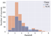 |
Fig. 1. LAEs (blue) and NLAEs (red) populations considered in the redshift range z ∈ [2, 7.9]. |
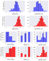 |
Fig. 2. Distributions of the physical parameters of the 1115 galaxies in the redshift range z ∈ [2.5, 4.5]. We show a direct comparison between LAEs (blue) and NLAEs (red). The thick and thin black lines correspond to the median, 25 percentile, and 75 percentile values of the distributions. |
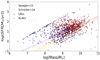 |
Fig. 3. Main sequence diagram of the 1115 galaxies in the redshift range z ∈ [2.5, 4.5]. The yellow dot-dashed line indicates the best fit relation Schreiber et al. (2015) at z = 3.5, the continuous yellow lines refer to the fits at z = 2.5 and z = 4.5. The pink dashed line indicates the fit by Speagle et al. (2014) at z = 3.5, while the continuous pink lines refer to the fits at z = 2.5 and z = 4.5. |
In Figs. 5–8, we present the variation of the Lyα EW as a function of the stellar mass, SFR, reddening, and half-light semi-major axis, Re. For reference, in each plot we indicate the EW = 20 Å threshold with a horizontal black dashed line.
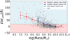 |
Fig. 5. Lyα EW vs. total stellar mass estimates. The horizontal black dashed line shows the 20 Å threshold a source has to exceed to be considered a LAE. For readability, the blue and red portions of the figure mark LAE and NLAE populations respectively. Red, blue, and green trends represent respectively the EW median values in Mass bin of 0.5 dex for GOODS-S, COSMOS, and UDS fields. They are associated with an error bar, accounting for the median absolute deviation. |
In Fig. 5, we show that the stellar mass tends to be higher for sources with lower Lyα EW. We also show median values in mass bins of 0.5 dex separately for GOODS-S (in red), COSMOS (in blue), and UDS (in green) to check whether any systematic is present. The plot shows that GOODS-S, being the field with the deepest photometry comprises many low mass faint galaxies. Typically, LAEs are galaxies with stellar mass lower than 109 M⊙, similar to what reported by Ouchi et al. (2020). We also find there are few LAEs which have stellar mass in excess of M ≥ 1010 M⊙, in good agreement with the results presented by Hagen et al. (2014).
From Fig. 6, we can see that LAEs typically are galaxies which show an SFR lower than few solar masses per year ≤ 100.5 − 10 M⊙ yr−1. This result is in agreement with the one reported by Ouchi et al. (2020; ∼1 − 10 M⊙ yr−1). From Fig. 7, we can see that as expected the emission line becomes progressively fainter as the dust content increases. On average, LAEs show little dust content, with typical reddening E(B − V)∼0 − 0.2 and a median value of 0.06, since Lyα can be easily suppressed by dust present in a galaxy. A null reddening is reported by Ono et al. (2010) on a population of ∼600 LAEs selected with narrow band techniques, while Kojima et al. (2017) found the same reddening range obtained in our work. However as already found by Hagen et al. (2014), we notice that there are also some LAEs that show larger reddening values, exceeding 0.3. This might be due, for example, to a displacement between regions from which stellar and nebular flux originate or to a non-uniform distribution of dust which could differentially suppress UV photons and not Lyα as first discussed by Neufeld (1991). Finally, in Fig. 8, we show the variation of the Lyα EW as a function of the half-light semi-major axis, Re. Even though the three median trends associated to the different fields are the most scattered relations amongst the properties studied, LAEs are very compact galaxies which (on average) have smaller Re values than NLAEs do. This is in agreement with the result found in a number of previous works (see also Taniguchi et al. 2009; Malhotra et al. 2012; Paulino-Afonso et al. 2018).
To quantify all the correlations described above, we ran a Spearman rank test (Spearman 1904) between the Lyα EW and the physical and morphological properties of the galaxies. We note that this test assesses whether a monotonic relation exist between two variables, without any assumptions on the form of the relation. The relevant p-value p(rs) is the probability of the null hypothesis of absence of any correlation. We consider a correlation to be present whenever p(rs) < 0.01. The results on our sample are shown in Fig. 9 and reported in Table 3: we see that all features show anti-correlations, except for the Sèrsic index which is positively correlated and for the age, whose p-value is > 0.01, thus the no correlation scenario could not be discarded. The stellar mass, reddening, SFR, and the half-light semi-major axis are found to be the features that correlate more strongly with the observed Lyα EW. Similar results on the strong correlation of the Lyα EW with stellar mass, SFR, and dust extinction were previously found by many works (e.g., Kornei et al. 2010; Pentericci et al. 2010; Oyarzún et al. 2017; Du et al. 2018; Marchi et al. 2019; McCarron et al. 2022; Chavez Ortiz et al. 2023).
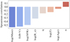 |
Fig. 9. Spearman correlation coefficients between the Lyα EW and each physical and morphological feature, calculated on the 1115 galaxies which reside in the redshift range z ∈ [2.5, 4.5] and are associated to a direct measure of Lyα EW. |
Spearman correlation coefficients with the Lyα EW.
In the next section, we try to exploit the above correlations to build a ML algorithm that can identify LAEs only on the basis of the physical and morphological properties (which can be derived by multi-wavelength photometry), without the need for costly spectroscopic observations.
5. RF classifier
We developed a ML classifier aimed at distinguishing LAEs from NLAEs, namely, a binary class problem in which the target labels (LAEs/NLAEs) are discrete. We opted for a supervised approach because we want to use all the physical, morphological, and spectroscopic data available from the GOODS-S, COSMOS, and UDS fields. The task of learning consists in mapping features (i.e., physical and morphological properties) to class labels (i.e., LAEs/NLAEs identification thanks to spectroscopic data), based on training example pairs (i.e., features and labels shown to the classifier). To train the ML methods on the classification task of selecting LAEs, we employed only the spectroscopic labels (LAEs and NLAEs) without directly using the specific information about the Lyα line flux and EW.
5.1. Brief overview of the RF classifier
Random forest (Breiman 2001) is a publicly available scikit-learn (Pedregosa et al. 2011) ensemble learning classifier that combines multiple decision trees to improve classification performance. Each tree in the forest is built on a random subset of the training data. During prediction, each tree votes for the class label and the final prediction of the ensemble classifier is the majority vote of all the trees. The general idea beneath a single tree classifier consists in finding the optimal set of rules to partition the space of features to distinguish data points of different classes. A single tree-classifier works in such a way that each time a new rule is applied, the data set splits into two new branches, creating a node. Because this process is recursive, the decision graph resembles the schema of an upside-down tree. The root node at the top of a decision tree contains the entire data set. At each branch of the tree, data are divided into two child nodes subsets, based on a decision boundary: one node contains data below the decision threshold and the other one includes data above it. Geometrically speaking, boundaries are hyper-surfaces axes aligned in the space of features. The splitting process repeats until a predefined stopping criteria is achieved in the leaves nodes, where all data contained are finally catalogued with just one class label, namely, the most recurrent label in the subset associated to the terminal leaf node itself. The fraction of samples of the same class in all the leaf nodes is also used as the class probability output for the objects classified. The application of a single decision tree for classifying new unlabeled data consists in following the tree’s branches through a series of binary decisions until a leaf node is reached. Training a decision tree algorithm on a labeled data set means finding the optimal order of rules to minimize the number of objects not correctly classified. This is done trying to maximize purity in each node, namely, an indicator that the considered subset contains predominantly observations from a single class. To measure the purity, the Gini index is commonly adopted: it estimates the probability that a randomly selected source would be incorrectly classified in the subset node if its label was drawn randomly, based on the label distribution of the same data subset.
Single decision trees are prone to overfitting: as the splitting process progresses thanks to the rule set by the Gini index, the error on the training set will decrease; however, at some point in its growth, the tree will cease to represent the correlations within data and will reflect the noise within the training set. The core idea of the RF method is thus to introduce random perturbations into the learning procedure of an ensemble of tree classifiers to obtain several different models from a single learning set. This is achieved during training through the hyper-parameters (i.e., internal parameters to be set by the user) of the method: their role is to control the growth of each decision tree and to introduce random perturbation in the splitting process. The final prediction is then obtained combining the results of the whole ensemble of classifiers: the class of each object is determined by a majority vote among all the trees. The RF classifier also outputs the class probability associated to each object through the internal method predict_proba. The predicted class probabilities of an input sample are computed as the mean predicted class probabilities of the trees in the forest.
5.2. Training the optimal RF classifier
The search for the optimal set of hyper-parameters which fully describes the optimal RF classifier was performed by a “5 k-fold cross validation” approach and through a standard grid search. The optimal classifier is defined as the RF that maximizes the cross-validation set accuracy, namely, the average fraction of the galaxies correctly classified on the cross-validating sets. When applied to boolean data, using the definition of true positives (TP), false positives (FP), true negatives (TN), and false negatives (FN), the accuracy score is expressed as (TP + TN)/(TP + FP + TN + FN). In our case, TP and TN are, respectively, the number of sources that belong to LAEs and NLAEs classes in both spectroscopic data and algorithm guesses; FP is the number of sources labeled as LAEs by the algorithm but being NLAEs in the truth; finally, FN is the number of sources that belong to the LAEs target class according to the spectroscopic data and mis-guessed by the ML algorithm. Precision refers to the fraction of truly LAEs predictions over all data predicted as LAEs by the RF classifier (TP/(TP + FP)), is a scoring metric that was also monitored through training and testing, but was not considered for the search of the optimal classifier.
Through the grid search, we explored the most critical hyper-parameters of the method that regulate the growth of the forest during training. First, “n_estimators” are the total number of trees in the forest. The more decision trees, the more opportunities the algorithm has to learn from a variety of features and subset combinations. However after exceeding a threshold, new trees do not reveal any more information because they get highly correlated with each other. This parameter varied in our grid between 50 and 600 (in multiples of 50). Then, “max_depth” is the maximum depth for each tree in the splitting process. This parameter, which controls the classifying capability of each tree, varied between 5 and 30 (in multiples of 5). Finally, “max_features” is the number of features to consider when looking for the best split in the splitting process. It is of key importance for growing trees slightly different from each other. Uncorrelated trees make the majority voting process of the forest more robust. We note that the forest, as an ensemble, is guaranteed to use all the features in the dataset. This parameter assumes all values between 2 and 8, namely, up to the total number of features we have in our dataset.
The final grid explored contains ∼500 models. A key aspect during training was setting the hyper-parameter class_weight = “balanced_subsample” such that for every tree grown during the training, learning weights associated to the input data were inversely proportional to class frequencies. This prevents the algorithm to be biased to classify correctly only the NLAEs majority class. The other hyper-parameters, which controls the branching of each tree were left as default: min_samples_split = 2, min_samples_leaf = 1. The first one controls the minimum number of samples required to split a parent node into two child nodes, while the latter sets the minimum number of samples required to be at a leaf node. In other words, a split point at any depth will only be considered if the parent node holds more than min_samples_split data and it leaves at least min_samples_leaf training samples in each of the left and right branches. These additional requirements are also referred to as the “pruning technique”. By setting these two hyper-parameters to the recommended default values, we consider an ensemble of unpruned trees (see the scikit-learn Pedregosa et al. 2011 website2 for a detailed reference).
To search for the optimal classifier the training+validating dataset has been chosen to be the 80% of the 1115 galaxies in the redshift range z ∈ [2.5, 4.5], while the remaining sources (20%) have been used as a test set to check the results. The standard decision of partitioning the training+validating dataset in “5 folds” ensures to have a validation set size that is comparable to the test data. The splitting was performed choosing a fixed random seed, such that the fraction of LAEs in the training and test set would remain similar to the percentage of LAEs (33.4%) in the complete dataset (see Table 4). We used the same internal random seed to get reproducible results. The best performances achieved by maximizing the cross-validation set accuracy were obtained when setting the following hyper-parameters: n_estimators = 500, max_depth = 20, and max_features = 3. This optimal RF classifier achieves accuracy values of (79.4 ± 3.6)% and 82.5% for the cross-validation and test set, respectively. The scores for the precision are (74.4 ± 8.2)% and 79.0% for the cross-validation and test set respectively. The uncertainty on cross-validation results is the standard deviation on the “5 folds”, while the test results do not have an uncertainty, given we are dealing with a single sample. Maximizing precision instead of accuracy over the cross-validation set does not change the results significantly. We note that the final accuracies obtained are comparable to those reached by narrow band selected samples, whose contamination rates range from few to 30%, depending on redshift and magnitude limit (Ouchi et al. 2018). In Fig. 10 (from the upper-left to lower-right), we report the confusion matrix values accounting for the TN, FP, FN, and TP in the test set of 223 galaxies. In Fig. 11, we highlight the most important features used for the classification task during training: the order of importance is in very good agreement with the absolute values of the Spearman correlation coefficients found between the Lyα EW and the features analyzed (Fig. 9). This proves that the RF method builds on these correlations and succeeds in recognizing that Lyα emitters tend to be low-mass, low-SFR galaxies that have little dust content and very compact sizes. The galaxies’ orientation with respect to the line of sight, accounted by the projected axis ratio, q, represents the middle point in order of importance of the presented correlations found both from the Spearman test within data and the RF classifier. The remaining features (Sérsic index, age, and metallicity) fall behind in terms of significance.
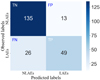 |
Fig. 10. Confusion matrix computed on the test set. From the upper left to lower right in order the total number of TN, FP, FN, and TP are reported. The total number of galaxies in the test set is 223. |
Training and test sets considered in the search of the optimal model’s hyper-parameters.
5.3. Misclassified objects
We further investigated the causes that would make the RF misclassify 26 LAEs (FN sample) by comparing the median values of this sample with the ones related to the LAEs showed during training. The FN sample and the LAEs in the training set respectively have median log(Mass) of 9.1 and 8.8, log(SFR) of 1.1 and 0.8, E(B − V) of 0.10 and 0.06, and log(Re) of 0.08 and 0.05. The FN sample is thus composed of LAEs, whose stellar mass, SFR, reddening, and half-light semi-major axis values are all higher than the ones of the LAEs in the training. Since those are the most important features (Fig. 11) that the RF tool is using for classification, the method gets misled and fails to recognize them.
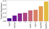 |
Fig. 11. Ranking of the most important features used by the optimal RF classifier method during its training. |
A similar analysis was conducted for the 13 galaxies misclassified as LAEs (FP sample) by inspecting the most important features. These galaxies have median log(Mass) of 8.7, log(SFR) of 0.8, E(B − V) of 0.1, and log(Re) of 0.07, at variance with the median values of the NLAEs population shown during training (median log(Mass) of 9.4, log(SFR) of 1.4, E(B − V) of 0.15 and log(Re) of 0.25). The FP sample seems to be composed of peculiar NLAEs with smaller values of stellar mass, SFR, reddening, and half-light semi-major axis than the ones shown during training.
The RF tool tends to misclassify galaxies with intermediate properties in the test sample. To improve the results from this method, a larger training set set would be needed. Our results would also benefit from adding further properties that could be derived from photometry and that should be correlated (or anticorrelated) with the Lyα equivalent width. For example we could add the ξion, namely, the ionizing photon production efficiency, which is given as output by some SED fitting codes (e.g., BEAGLE; Chevallard & Charlot 2016) and has been found to strongly correlate with the Lyα emission strength, as recently shown by Castellano et al. (2023). This would help in distinguishing LAEs from NLAEs when the other features have intermediate values, as in the cases discussed for the FP and FN samples.
We investigated which is the minimum probability to set when looking at all the positive predictions, in order to get only TP i.e. maximising the purity of the predictions to 100%. To this aim, we used the predict_proba method provided for the classifier (described in Sect. 5.1). We found that with a 0.93 cut in probability of being a LAE, the classifier finds only true positive (LAEs). However in this way we would lose as many as ∼84% of the real LAEs as well, thereby resulting in a very limited final sample.
5.4. Testing the solidity of the optimal RF
The test set result obtained by searching for the optimal RF classifier is linked to the particular sub-division in the training and test datasets, performed when splitting data through the fixed random seed chosen. We thus evaluated the solidity of the optimal RF (n_estimators = 500, max_depth = 20, and max_features = 3; see Sect. 5.2) by creating 100 different training and test sets (with 80% and 20% ratios) through 100 unique shuffling seeds applied to our sample of 1115 galaxies. In this iteration process we required the two subsets to have roughly the same LAEs percentage as the whole dataset. Since we have already determined the optimal RF, in this procedure, we do not need a validation set. The average results on the 100 test sets for accuracy and precision are respectively (79.7 ± 2.1)% and (73.1 ± 4.3)% in good agreement with the results obtained during the cross-validation process. The uncertainties reported are the standard deviations derived from the 100 test sets.
One of the purposes of training the optimal RF classifier is to develop a robust method to select galaxies which have the highest probability of being Lyα emitters from photometric catalogs. We therefore tested the optimal classifier in the case where only the photometric information is available, namely, without the spectroscopic redshift information. For this purpose, we re-evaluated the physical properties of our sample through SED fitting by fixing the redshift of each source to the photometric estimate (Kodra et al. 2023) and following the same procedure described in Sect. 3.1. We then defined the training+validating (test) dataset as the 80% (20%) of the 1081 galaxies in the redshift range of zphot ∈ [2.5, 4.5]. We note that by using the photometric redshifts, we lost 34 previously considered galaxies, (∼3% of the total). Using the same procedure described in Sect. 5.2, we re-trained and tested the optimal RF on this new dataset, achieving a test accuracy and precision of 82.0% and 81.1%, respectively. These values are in very good agreement with the results previously obtained both in Sects. 5.2 and 5.4. In turn, this shows that the classification does not suffer from the uncertainties derived from an SED fitting based on the photometric redshifts instead of the spectroscopic ones, as also shown by several works (Merlin et al. 2021; Kodra et al. 2023; Arrabal Haro et al. 2023).
In Sect. 2.3 we described how we assembled the largest possible spectroscopic sample by considering 11 different observational programs. In each of these surveys targets were pre-selected using different criteria (colour selection and/or photometric redshifts). Clearly, this could cause selection biases in the final sample, which are difficult to assess. To evaluate how the different selection functions could affect our results we carried out two different tests:
First, we trained and tested the optimal classifier on just one survey – namely, a subset with a unique selection function. We considered the VANDELS survey because it is the only subset with enough data (555 galaxies in the redshift range z ∈ [2.5, 4.5]) which could be then split into the training and test samples (80% and 20% respectively). After applying the same procedure described in Sect. 5.2, we obtained a 79.3% test accuracy, consistent with results obtained with the entire sample.
Second, we trained the optimal classifier on all the data, except for a survey to be left as the test set. We note that this resembles the possible case in which the optimal classifier trained in Sect. 5.2 would be applied to an independent data set from a new survey with a different pre-selection. We used the combined GOODS-S VIMOS and GOODS-S FORS samples as the test set (given that they were selected in the same way). In this case, we used 982 galaxies for the training and 133 for testing the performances, with a training-test ratio that is roughly 90%–10%. We obtained an 82.7% test accuracy again consistent with the results on the entire sample.
In conclusion, although our tests are not exhaustive, we find that the different selection effects do not change substantially the efficiency of the optimal algorithm. This is probably due to the fact that current photometric redshift codes in general are rather robust and in reasonable agreement with each other, especially for star forming galaxies in the redshift range where we carried out our training process.
5.5. Application of the optimal method to higher redshift
Finally, we applied the optimal classifier on the 194 galaxies in our initial sample with redshifts between 4.5 and 6. This sample contains a higher fraction (53.6%) of LAEs, compared to the one used in our training and test. As already mentioned in the introduction, this is due both to an evolution in the intrinsic galaxy properties and to an observational effect, since spectroscopic surveys can constrain only emission lines brighter than a limiting flux from galaxies. Since galaxies get fainter at increasingly high redshift, at some point, we end up with a bias toward the confirmation of the redshift more easily in the presence of a Lyα emission. In Fig. A.2, we show the completeness of our sample, finding that many surveys are not complete at the faint end. Applying the optimal algorithm to this completely independent dataset leads to a 73.2 % accuracy and 80.2 % precision. The lower accuracy obtained can be caused by the partial completeness in terms of spectroscopic identification of this sample.
In any case, the high precision achieved indicates the possibility of using our trained method for identifying LAE candidates during the EoR, where observations of large samples would be needed, for instance, to map the spatial inhomogeneous distribution of the neutral hydrogen fraction in the IGM (Yoshioka et al. 2022). Assuming a 50% (25%) of Lyα transmission due to a moderately neutral (highly neutral) IGM at z ≃ 7, if we optimally selected our spectroscopic candidates using our method (which has an 80% precision), we would obtain ≃40% (20%) LAEs detection rate; this is much higher than current detection rates at z ≃ 7 galaxies (Pentericci et al. 2018). This would open up the possibility of distinguishing more easily amongst regions with high or low neutral hydrogen content in the IGM. In addition also other types of Lyα diagnostics that probe cosmic reionization, such as an emission line shape analysis (Ouchi et al. 2020), could be carried out with much larger samples.
6. Summary and conclusions
Searching for LAEs at high-redshift is a challenging task due to both the limitations of the narrow-band deep imaging surveys and the time constraints to be faced when planning a blind spectroscopic survey. In this work, we present a new and efficient method based on machine learning (ML), which builds on the correlations found in the high-redshift star-forming galaxies between the strength of the Lyα emission and physical and morphological properties from multi-wavelength photometry. The aim was to select galaxies with the highest probability of being Lyα emitters.
We initially assembled a very large sample of 1578 galaxies at z ∈ [2, 7.9] selected from the CANDELS GOODS-S, COSMOS, and UDS fields. For these we also had access to deep spectroscopic observations, including the Lyα emission, as well as accurate physical and morphological properties derived in an homogeneous way from multi-wavelength photometry. We then considered galaxies in the redshift range z ∈ [2.5, 4.5], where the statistics is higher and where the spectroscopic surveys are complete for the identification of Lyα emission with EW ≥ 20 Å. This selected sample of 1115 sources, is mainly formed by star-forming galaxies on the main sequence (MS), in agreement with the best fit MS relation found in literature (Speagle et al. 2014; Schreiber et al. 2015). We find that the strength of the Lyα emission is strongly correlated with stellar mass, dust content, SFR, and half-light radius, in the sense that the line tends to be brighter for galaxies with small stellar mass, low SFR, low dust content, and a small radius, as has already been found by previous authors (Taniguchi et al. 2009; Ono et al. 2010; Malhotra et al. 2012; Hagen et al. 2014; Kojima et al. 2017; Paulino-Afonso et al. 2018; Ouchi et al. 2020). In turn, this can be explained by the major importance of the neutral hydrogen column density and the dust content within the inter-stellar medium in determining the rate of escape of Lyα photons from a galaxy. We find that the galaxy orientation with respect to the line of sight is only mildly correlated to the Lyα emission line. This suggests a scenario in which the preferential channels in the inter-stellar medium through which Lyα photons escape without getting absorbed by dust are mildly dependent of the particular galaxy orientation.
We then trained a RF classifier on the task of identifying LAEs by using all the physical and morphological information available, namely, eight features in total. The search of the optimal RF classifier was performed by a “5 k-fold cross-validation” approach and through a standard grid-search. Our best results were obtained by setting the following hyper-parameters: n_estimators = 500, max_depth = 20, max_features = 3, min_samples_split = 2, and min_samples_leaf = 1. This optimally trained classifier, when applied to an independent set of galaxies in the same redshift range as the training set, recovers true LAEs with a (79.7 ± 2.1)% accuracy and (73.1 ± 4.3)% precision.
The method could be further refined both by enlarging the training set to contain more numerous and more diverse galaxies, and by adding other predictive features, namely, properties that can also be correlated with the Lyα strength. One possibility could be the ionizing photon production efficiency, ξion, which was found to be correlated with the Lyα equivalent width (Harikane et al. 2018; Castellano et al. 2023). This could help the method to be more robust to false classification of galaxies with intermediate properties, as also suggested by our analysis of the misclassified objects.
When applying the classifier to a higher redshift z ∈ [4.5, 6] dataset of 194 galaxies, we obtained a slightly lower accuracy of 73.2%, but a precision as high as 80.2%. The RF classifier is therefore successful at selecting LAEs at high redshift and could be used to optimally plan spectroscopic follow-up observations in fields which boast good multi-wavelength photometric observations. This would allow us to maximize our chances of detecting galaxies with Lyα emission that are one of the best tools to study the EoR. As an example, our algorithm could be applied to future high redshift target selection with MOONS, the next-generation spectrograph for the VLT. With its large FoV and very high multiplexing capabilities, it will offer the possibility of obtaining the spectra of hundreds of high redshift galaxies in the EoR (Maiolino et al. 2020). MOONS will be able to observe the Lyα emission throughout all phases of reionization. With a survey tailored at maximizing the high redshift galaxies (z ≥ 6) which should intrinsically have strong Lyα emission, as selected by our algorithm, we could easily distinguish between regions that have a large IGM transmission (i.e., regions that are already highly ionized) from regions where the final escaping Lyα is very reduced due the high fraction of IGM neutral hydrogen content. We could therefore directly analyze the patchy spatial distribution of neutral hydrogen and compare it to the predictions from the simulations.
Acknowledgments
We thank the referee for the constructive feedback provided. We acknowledge support from INAF mainstream program VANDELS. L.N. thanks Stefano Giagu and Viviana Acquaviva for giving useful insights into the machine learning classification.
References
- Ajiki, M., Taniguchi, Y., Fujita, S. S., et al. 2003, AJ, 126, 2091 [NASA ADS] [CrossRef] [Google Scholar]
- Arrabal Haro, P., Dickinson, M., Finkelstein, S. L., et al. 2023, ApJ, 951, L22 [NASA ADS] [CrossRef] [Google Scholar]
- Balestra, I., Mainieri, V., Popesso, P., et al. 2010, A&A, 512, A12 [NASA ADS] [CrossRef] [EDP Sciences] [Google Scholar]
- Behrens, C., & Braun, H. 2014, A&A, 572, A74 [NASA ADS] [CrossRef] [EDP Sciences] [Google Scholar]
- Breiman, L. 2001, Machine Learning, 45, 5 [NASA ADS] [CrossRef] [Google Scholar]
- Bruzual, G., & Charlot, S. 2003, MNRAS, 344, 1000 [NASA ADS] [CrossRef] [Google Scholar]
- Calzetti, D., Armus, L., Bohlin, R. C., et al. 2000, ApJ, 533, 682 [NASA ADS] [CrossRef] [Google Scholar]
- Cassata, P., Tasca, L. A. M., Le Fèvre, O., et al. 2015, A&A, 573, A24 [NASA ADS] [CrossRef] [EDP Sciences] [Google Scholar]
- Castellano, M., Sommariva, V., Fontana, A., et al. 2014, A&A, 566, A19 [NASA ADS] [CrossRef] [EDP Sciences] [Google Scholar]
- Castellano, M., Belfiori, D., Pentericci, L., et al. 2023, A&A, 675, A121 [NASA ADS] [CrossRef] [EDP Sciences] [Google Scholar]
- Chabrier, G. 2003, PASP, 115, 763 [Google Scholar]
- Chavez Ortiz, O. A., Finkelstein, S. L., Davis, D., et al. 2023, ApJ, 952, 110 [NASA ADS] [CrossRef] [Google Scholar]
- Chen, C. T. J., Brandt, W. N., Reines, A. E., et al. 2017, ApJ, 837, 48 [NASA ADS] [CrossRef] [Google Scholar]
- Chevallard, J., & Charlot, S. 2016, MNRAS, 462, 1415 [NASA ADS] [CrossRef] [Google Scholar]
- Ciardullo, R., Feldmeier, J. J., Krelove, K., Jacoby, G. H., & Gronwall, C. 2002, ApJ, 566, 784 [NASA ADS] [CrossRef] [Google Scholar]
- Cornachione, M. A., Bolton, A. S., Shu, Y., et al. 2018, ApJ, 853, 148 [NASA ADS] [CrossRef] [Google Scholar]
- Cowie, L. L., & Hu, E. M. 1998, AJ, 115, 1319 [Google Scholar]
- Dijkstra, M. 2017, ArXiv e-prints [arXiv:1704.03416] [Google Scholar]
- Drake, A. B., Garel, T., Wisotzki, L., et al. 2017, A&A, 608, A6 [NASA ADS] [CrossRef] [EDP Sciences] [Google Scholar]
- Du, X., Shapley, A. E., Reddy, N. A., et al. 2018, ApJ, 860, 75 [NASA ADS] [CrossRef] [Google Scholar]
- Dunlop, J. S. 2013, Astrophys. Space Sci. Lib., 396, 223 [NASA ADS] [CrossRef] [Google Scholar]
- Dunlop, J. S., Rogers, A. B., McLure, R. J., et al. 2013, MNRAS, 432, 3520 [NASA ADS] [CrossRef] [Google Scholar]
- Fontana, A., D’Odorico, S., Poli, F., et al. 2000, AJ, 120, 2206 [NASA ADS] [CrossRef] [Google Scholar]
- Fujita, S. S., Ajiki, M., Shioya, Y., et al. 2003, AJ, 125, 13 [NASA ADS] [CrossRef] [Google Scholar]
- Fynbo, J. U., Møller, P., & Thomsen, B. 2001, A&A, 374, 443 [NASA ADS] [CrossRef] [EDP Sciences] [Google Scholar]
- Fynbo, J. P. U., Ledoux, C., Møller, P., Thomsen, B., & Burud, I. 2003, A&A, 407, 147 [NASA ADS] [CrossRef] [EDP Sciences] [Google Scholar]
- Galametz, A., Grazian, A., Fontana, A., et al. 2013, ApJS, 206, 10 [Google Scholar]
- Garilli, B., McLure, R., Pentericci, L., et al. 2021, A&A, 647, A150 [NASA ADS] [CrossRef] [EDP Sciences] [Google Scholar]
- Grogin, N. A., Kocevski, D. D., Faber, S. M., et al. 2011, ApJS, 197, 35 [NASA ADS] [CrossRef] [Google Scholar]
- Gronwall, C., Ciardullo, R., Hickey, T., et al. 2007, ApJ, 667, 79 [NASA ADS] [CrossRef] [Google Scholar]
- Grove, L. F., Fynbo, J. P. U., Ledoux, C., et al. 2009, A&A, 497, 689 [NASA ADS] [CrossRef] [EDP Sciences] [Google Scholar]
- Gurung-López, S., Gronke, M., Saito, S., Bonoli, S., & Orsi, Á. A. 2022, MNRAS, 510, 4525 [NASA ADS] [CrossRef] [Google Scholar]
- Hagen, A., Ciardullo, R., Gronwall, C., et al. 2014, ApJ, 786, 59 [NASA ADS] [CrossRef] [Google Scholar]
- Harikane, Y., Ouchi, M., Shibuya, T., et al. 2018, ApJ, 859, 84 [NASA ADS] [CrossRef] [Google Scholar]
- Hasinger, G., Capak, P., Salvato, M., et al. 2018, ApJ, 858, 77 [Google Scholar]
- Hayashino, T., Matsuda, Y., Tamura, H., et al. 2004, AJ, 128, 2073 [Google Scholar]
- Jensen, H., Laursen, P., Mellema, G., et al. 2013, MNRAS, 428, 1366 [CrossRef] [Google Scholar]
- Kashino, D., Lilly, S. J., Renzini, A., et al. 2022, ApJ, 925, 82 [NASA ADS] [CrossRef] [Google Scholar]
- Kocevski, D. D., Hasinger, G., Brightman, M., et al. 2018, ApJS, 236, 48 [CrossRef] [Google Scholar]
- Kodra, D., Andrews, B. H., Newman, J. A., et al. 2023, ApJ, 942, 36 [NASA ADS] [CrossRef] [Google Scholar]
- Koekemoer, A. M., Faber, S. M., Ferguson, H. C., et al. 2011, ApJS, 197, 36 [NASA ADS] [CrossRef] [Google Scholar]
- Kojima, T., Ouchi, M., Nakajima, K., et al. 2017, PASJ, 69, 44 [NASA ADS] [CrossRef] [Google Scholar]
- Kornei, K. A., Shapley, A. E., Erb, D. K., et al. 2010, ApJ, 711, 693 [NASA ADS] [CrossRef] [Google Scholar]
- Kurk, J., Cimatti, A., Daddi, E., et al. 2013, A&A, 549, A63 [NASA ADS] [CrossRef] [EDP Sciences] [Google Scholar]
- Le Fèvre, O., Tasca, L. A. M., Cassata, P., et al. 2015, A&A, 576, A79 [Google Scholar]
- Lilly, S. J., Le Fèvre, O., Renzini, A., et al. 2007, ApJS, 172, 70 [Google Scholar]
- Luo, B., Brandt, W. N., Xue, Y. Q., et al. 2017, ApJS, 228, 2 [Google Scholar]
- Maiolino, R., Cirasuolo, M., Afonso, J., et al. 2020, The Messenger, 180, 24 [NASA ADS] [Google Scholar]
- Malhotra, S., Rhoads, J. E., Finkelstein, S. L., et al. 2012, ApJ, 750, L36 [NASA ADS] [CrossRef] [Google Scholar]
- Marchi, F., Pentericci, L., Guaita, L., et al. 2019, A&A, 631, A19 [NASA ADS] [CrossRef] [EDP Sciences] [Google Scholar]
- Markwardt, C. B. 2009, ASP Conf. Ser., 411, 251 [Google Scholar]
- McCarron, A. P., Finkelstein, S. L., Chavez Ortiz, O. A., et al. 2022, ApJ, 936, 131 [NASA ADS] [CrossRef] [Google Scholar]
- McLure, R. J., Pentericci, L., Cimatti, A., et al. 2018, MNRAS, 479, 25 [NASA ADS] [Google Scholar]
- Merlin, E., Castellano, M., Santini, P., et al. 2021, A&A, 649, A22 [NASA ADS] [CrossRef] [EDP Sciences] [Google Scholar]
- Mukherjee, S., Bhattacharjee, A., Chatterjee, S., Newman, J. A., & Yan, R. 2019, ApJ, 872, 35 [NASA ADS] [CrossRef] [Google Scholar]
- Nakajima, K., Ouchi, M., Shimasaku, K., et al. 2012, Am. Astron. Soc. Meet. Abstr., 220, 429.01 [NASA ADS] [Google Scholar]
- Nayyeri, H., Hemmati, S., Mobasher, B., et al. 2017, ApJS, 228, 7 [NASA ADS] [CrossRef] [Google Scholar]
- Neufeld, D. A. 1991, ApJ, 370, L85 [Google Scholar]
- Ono, Y., Ouchi, M., Shimasaku, K., et al. 2010, ApJ, 724, 1524 [NASA ADS] [CrossRef] [Google Scholar]
- Ono, Y., Itoh, R., Shibuya, T., et al. 2021, ApJ, 911, 78 [NASA ADS] [CrossRef] [Google Scholar]
- Ouchi, M., Shimasaku, K., Furusawa, H., et al. 2003, ApJ, 582, 60 [Google Scholar]
- Ouchi, M., Shimasaku, K., Furusawa, H., et al. 2010, ApJ, 723, 869 [Google Scholar]
- Ouchi, M., Harikane, Y., Shibuya, T., et al. 2018, PASJ, 70, S13 [Google Scholar]
- Ouchi, M., Ono, Y., & Shibuya, T. 2020, ARA&A, 58, 617 [Google Scholar]
- Oyarzún, G. A., Blanc, G. A., González, V., Mateo, M., & Bailey, J. I. 2017, ApJ, 843, 133 [CrossRef] [Google Scholar]
- Paulino-Afonso, A., Sobral, D., Ribeiro, B., et al. 2018, MNRAS, 476, 5479 [NASA ADS] [CrossRef] [Google Scholar]
- Pedregosa, F., Varoquaux, G., Gramfort, A., et al. 2011, J. Mach. Learn. Res., 12, 2825 [Google Scholar]
- Pentericci, L., Grazian, A., Fontana, A., et al. 2009, A&A, 494, 553 [NASA ADS] [CrossRef] [EDP Sciences] [Google Scholar]
- Pentericci, L., Grazian, A., Scarlata, C., et al. 2010, A&A, 514, A64 [NASA ADS] [CrossRef] [EDP Sciences] [Google Scholar]
- Pentericci, L., Fontana, A., Vanzella, E., et al. 2011, ApJ, 743, 132 [NASA ADS] [CrossRef] [Google Scholar]
- Pentericci, L., McLure, R. J., Garilli, B., et al. 2018, A&A, 616, A174 [NASA ADS] [CrossRef] [EDP Sciences] [Google Scholar]
- Popesso, P., Dickinson, M., Nonino, M., et al. 2009, A&A, 494, 443 [NASA ADS] [CrossRef] [EDP Sciences] [Google Scholar]
- Runnholm, A., Hayes, M., Melinder, J., et al. 2020, ApJ, 892, 48 [NASA ADS] [CrossRef] [Google Scholar]
- Santini, P., Ferguson, H. C., Fontana, A., et al. 2015, ApJ, 801, 97 [Google Scholar]
- Santini, P., Castellano, M., Fontana, A., et al. 2022, ApJ, 940, 135 [NASA ADS] [CrossRef] [Google Scholar]
- Saxena, A., Robertson, B. E., Bunker, A. J., et al. 2023, A&A, in press, https://doi.org/10.1051/0004-6361/202346245 [Google Scholar]
- Schaerer, D., & de Barros, S. 2009, A&A, 502, 423 [NASA ADS] [CrossRef] [EDP Sciences] [Google Scholar]
- Schmidt, K. B., Kerutt, J., Wisotzki, L., et al. 2021, A&A, 654, A80 [NASA ADS] [CrossRef] [EDP Sciences] [Google Scholar]
- Schreiber, C., Pannella, M., Elbaz, D., et al. 2015, A&A, 575, A74 [NASA ADS] [CrossRef] [EDP Sciences] [Google Scholar]
- Schreiber, C., Glazebrook, K., Nanayakkara, T., et al. 2018, A&A, 618, A85 [NASA ADS] [CrossRef] [EDP Sciences] [Google Scholar]
- Sersic, J. L. 1968, Atlas de Galaxias Australes (Cordoba, Argentina: Observatorio Astronomico) [Google Scholar]
- Shanmugasundararaj, K., Thomas, B., Robinson, E., et al. 2021, Am. Astron. Soc. Meet. Abstr., 135.06, 53 [NASA ADS] [Google Scholar]
- Shapley, A. E., Steidel, C. C., Adelberger, K. L., et al. 2001, ApJ, 562, 95 [NASA ADS] [CrossRef] [Google Scholar]
- Shibuya, T., Ouchi, M., Kubo, M., & Harikane, Y. 2016, ApJ, 821, 72 [NASA ADS] [CrossRef] [Google Scholar]
- Shibuya, T., Ouchi, M., Harikane, Y., & Nakajima, K. 2019, ApJ, 871, 164 [NASA ADS] [CrossRef] [Google Scholar]
- Smith, A., Ma, X., Bromm, V., et al. 2019, MNRAS, 484, 39 [NASA ADS] [CrossRef] [Google Scholar]
- Smith, A., Kannan, R., Tacchella, S., et al. 2022, MNRAS, 517, 1 [NASA ADS] [CrossRef] [Google Scholar]
- Speagle, J. S., Steinhardt, C. L., Capak, P. L., & Silverman, J. D. 2014, ApJS, 214, 15 [Google Scholar]
- Spearman, C. 1904, Am. J. Psychol., 15, 201 [CrossRef] [Google Scholar]
- Stark, D. P., Ellis, R. S., Chiu, K., Ouchi, M., & Bunker, A. 2010, MNRAS, 408, 1628 [Google Scholar]
- Steidel, C. C., Giavalisco, M., Pettini, M., Dickinson, M., & Adelberger, K. L. 1996, ApJ, 462, L17 [Google Scholar]
- Stiavelli, M., Scarlata, C., Panagia, N., et al. 2001, ApJ, 561, L37 [NASA ADS] [CrossRef] [Google Scholar]
- Talia, M., Schreiber, C., Garilli, B., et~al. 2023, A&A, in press, https://doi.org/10.1051/0004-6361/202346293 [Google Scholar]
- Taniguchi, Y., Ajiki, M., Nagao, T., et al. 2005, PASJ, 57, 165 [NASA ADS] [Google Scholar]
- Taniguchi, Y., Murayama, T., Scoville, N. Z., et al. 2009, ApJ, 701, 915 [NASA ADS] [CrossRef] [Google Scholar]
- Tasca, L. A. M., Le Fèvre, O., Ribeiro, B., et al. 2017, A&A, 600, A110 [NASA ADS] [CrossRef] [EDP Sciences] [Google Scholar]
- van der Wel, A., Bell, E. F., Häussler, B., et al. 2012, ApJS, 203, 24 [NASA ADS] [CrossRef] [Google Scholar]
- Vanzella, E., Cristiani, S., Dickinson, M., et al. 2008, A&A, 478, 83 [NASA ADS] [CrossRef] [EDP Sciences] [Google Scholar]
- Vanzella, E., Giavalisco, M., Dickinson, M., et al. 2009, ApJ, 695, 1163 [NASA ADS] [CrossRef] [Google Scholar]
- Verhamme, A., Dubois, Y., Blaizot, J., et al. 2012, A&A, 546, A111 [NASA ADS] [CrossRef] [EDP Sciences] [Google Scholar]
- Verhamme, A., Orlitová, I., Schaerer, D., & Hayes, M. 2015, A&A, 578, A7 [NASA ADS] [CrossRef] [EDP Sciences] [Google Scholar]
- Yoshioka, T., Kashikawa, N., Inoue, A. K., et al. 2022, ApJ, 927, 32 [NASA ADS] [CrossRef] [Google Scholar]
- Zheng, Z., Cen, R., Trac, H., & Miralda-Escudé, J. 2010, ApJ, 716, 574 [NASA ADS] [CrossRef] [Google Scholar]
Appendix A: Completeness of the surveys considered
In this appendix, we show the test performed in order to assess the completeness of our sample for each survey considered.
We first considered galaxies at 2.5 ≤ z ≤ 4.5, namely, the sample used for training our method. From the photometric catalogs (Galametz et al. 2013; Nayyeri et al. 2017; Merlin et al. 2021), we associated each survey with the magnitude range spanned for the F160W HST filter, where the continuum emission near to the Lyα line is redshifted. From the limiting (3σ) flux flim reported in Table 2 and assuming the mean redshift of the survey for each subsample, we then computed the limiting Lyα EW restframe. In Fig. A.1, we compare the limiting Lyα EW with the F606W magnitude range. Overall, in this redshift range our sample is > 99% complete down to the magnitude limit of each survey. The exception is MUSE-Wide whose limiting Lyα EW exceeds the 20 Å for magnitudes > 26.5. However, the number of these sources is limited compared to the 1115 galaxies in the data sample at this redshift range. Thus, losing some faint NLAEs for this survey does not affect our analysis.
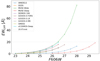 |
Fig. A.1. Limiting Lyα EW vs F606W magnitudes for galaxies at 2.5 ≤ z ≤ 4.5 derived from the limiting 3σ fluxes reported in Tab. 2. Each survey covers a different magnitude range, according to the galaxies targeted. The grey horizontal line shows the 20 Å threshold. |
In Fig. A.2, we report the limiting Lyα EW with the F814W magnitude range, for the subset of galaxies at 4.5 ≤ z ≤ 6. In this case, the F814W HST filter holds the information on the continuum emission near to the Lyα line. As a result, given the limiting (3σ) flux flim reported in Table 2, many surveys are not complete in the faint end population of galaxies. We decided not to include galaxies at this redshift range for training our method because of the partial completeness.
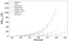 |
Fig. A.2. Limiting Lyα EW vs F814W magnitudes for galaxies at 4.5 ≤ z ≤ 6. Symbols are the same as in Fig. A.1 |
All Tables
Spectroscopic surveys with 3σ limiting flux in units of 10−18 erg s−1 cm−2 and redshift range.
Training and test sets considered in the search of the optimal model’s hyper-parameters.
All Figures
|
Fig. 1. LAEs (blue) and NLAEs (red) populations considered in the redshift range z ∈ [2, 7.9]. |
| In the text | |
|
Fig. 2. Distributions of the physical parameters of the 1115 galaxies in the redshift range z ∈ [2.5, 4.5]. We show a direct comparison between LAEs (blue) and NLAEs (red). The thick and thin black lines correspond to the median, 25 percentile, and 75 percentile values of the distributions. |
| In the text | |
|
Fig. 3. Main sequence diagram of the 1115 galaxies in the redshift range z ∈ [2.5, 4.5]. The yellow dot-dashed line indicates the best fit relation Schreiber et al. (2015) at z = 3.5, the continuous yellow lines refer to the fits at z = 2.5 and z = 4.5. The pink dashed line indicates the fit by Speagle et al. (2014) at z = 3.5, while the continuous pink lines refer to the fits at z = 2.5 and z = 4.5. |
| In the text | |
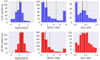 |
Fig. 4. Same as Fig. 2, but for the morphological properties Re, n, and q. |
| In the text | |
|
Fig. 5. Lyα EW vs. total stellar mass estimates. The horizontal black dashed line shows the 20 Å threshold a source has to exceed to be considered a LAE. For readability, the blue and red portions of the figure mark LAE and NLAE populations respectively. Red, blue, and green trends represent respectively the EW median values in Mass bin of 0.5 dex for GOODS-S, COSMOS, and UDS fields. They are associated with an error bar, accounting for the median absolute deviation. |
| In the text | |
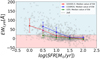 |
Fig. 6. Lyα EW vs. star formation rate. Symbols and colours are described in Fig. 5. |
| In the text | |
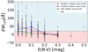 |
Fig. 7. Lyα EW vs. E(B − V). Symbols and colours are described in Fig. 5. |
| In the text | |
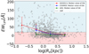 |
Fig. 8. Lyα EW vs. half-light semi-major axis Re. Symbols and colours are described in Fig. 5. |
| In the text | |
|
Fig. 9. Spearman correlation coefficients between the Lyα EW and each physical and morphological feature, calculated on the 1115 galaxies which reside in the redshift range z ∈ [2.5, 4.5] and are associated to a direct measure of Lyα EW. |
| In the text | |
|
Fig. 10. Confusion matrix computed on the test set. From the upper left to lower right in order the total number of TN, FP, FN, and TP are reported. The total number of galaxies in the test set is 223. |
| In the text | |
|
Fig. 11. Ranking of the most important features used by the optimal RF classifier method during its training. |
| In the text | |
|
Fig. A.1. Limiting Lyα EW vs F606W magnitudes for galaxies at 2.5 ≤ z ≤ 4.5 derived from the limiting 3σ fluxes reported in Tab. 2. Each survey covers a different magnitude range, according to the galaxies targeted. The grey horizontal line shows the 20 Å threshold. |
| In the text | |
|
Fig. A.2. Limiting Lyα EW vs F814W magnitudes for galaxies at 4.5 ≤ z ≤ 6. Symbols are the same as in Fig. A.1 |
| In the text | |
Current usage metrics show cumulative count of Article Views (full-text article views including HTML views, PDF and ePub downloads, according to the available data) and Abstracts Views on Vision4Press platform.
Data correspond to usage on the plateform after 2015. The current usage metrics is available 48-96 hours after online publication and is updated daily on week days.
Initial download of the metrics may take a while.