| Issue |
A&A
Volume 623, March 2019
|
|
|---|---|---|
| Article Number | A3 | |
| Number of page(s) | 26 | |
| Section | Stellar atmospheres | |
| DOI | https://doi.org/10.1051/0004-6361/201833738 | |
| Published online | 25 February 2019 | |
Surface abundances of CNO in Galactic O-stars: a pilot study with FASTWIND
1
LMU München, Universitätssternwarte,
Scheinerstr. 1,
81679 München, Germany
e-mail: luiz@usm.uni-muenchen.de
2
Instituto de Astrofísica de Canarias,
38200 La Laguna,
Tenerife, Spain
3
Departamento de Física y Astronomía, Universidad de La Laguna,
38205 La Laguna,
Tenerife, Spain
Received:
28
June
2018
Accepted:
21
November
2018
Context. Rotational mixing is known to significantly affect the evolution of massive stars; however, we still lack a consensus regarding the various possible modeling approaches and mixing recipes describing this process. The empirical investigation of surface abundances of carbon, nitrogen, and oxygen (CNO) in large samples of O- and B-type stars will be essential for providing meaningful observational constraints on the different available stellar evolution models.
Aims. Setting up and testing adequate tools to perform CNO surface abundance determinations for large samples of O-type stars, by means of the fast performance, NLTE, unified model atmosphere code FASTWIND.
Methods. We have developed a set of semi-automatic tools for measuring and analyzing the observed equivalent widths of strategic optical C, N, and O lines from different ions. Our analysis strategy is based on a χ2 minimization of weighted differences between observed and synthetic equivalent widths, the latter computed from tailored model grids. We have paid special attention to the (significant) errors introduced by typical uncertainties in stellar parameters. In this pilot study, we describe these tools, and test their performance and reliability using a set of high quality spectra of a sample of 18 presumably single Galactic O-type stars with low projected rotational velocities (v sin i≲100 km s−1), and previously determined stellar parameters. In particular, we have compared the outcome of our analysis with results from existing studies and theoretical stellar evolution models.
Results. Most of our results for carbon and nitrogen agree, within the errors, with both theoretical expectations and literature values. While many cooler dwarfs display C and N abundances close to solar, some of the early- and mid-O dwarfs – and most supergiants – show significant enrichment in N and depletion in C. Our results for oxygen in late-O dwarfs are, however, unexpectedly low, possibly indicating deficiencies in the adopted oxygen model atom. For all other objects, no systematic problems in their oxygen content have been identified. Specific stars in our sample show peculiarities in their abundances, and we suggest hypotheses regarding their origin.
Conclusions. Our method is (almost) ready to be applied to large samples of late and mid O-type stars – although the oxygen model atom needs to be improved and carefully tested first. For early O-type stars (O4 and hotter), a simultaneous UV analysis seems to be inevitable, due to the scarcity and weakness of optical C and O lines. This will necessarily imply a more complex modeling, additionally accounting for the effects of X-rays from wind-embedded shocks and wind inhomogeneities.
Key words: stars: early-type / stars: massive / stars: atmospheres / stars: abundances / stars: evolution
© ESO 2019
1. Introduction
Nucleosynthesis is the primary agent that controls stellar evolution. Although the nuclear processes are well understood, the transport and mixing (if there is any) of nuclear processed material into the envelope and stellar surface is still disputed. If present, such mixing is significant not only because it alters the surface abundances, but also, for example, since it might change the mean molecular weight and opacity, giving rise to larger convective cores and higher luminosities (see Maeder 2009).
In massive stars, this transport can be particularly strong, mostly due to rotational mixing (e.g., Langer et al. 1997; Meynet & Maeder 2000; Heger et al. 2000; Paxton et al. 2013): rotation may trigger internal instabilities, leading to flows that transport material from the core to the stellar surface and vice versa. Indeed, many massive stars are rapidly rotating (e.g., Howarth et al. 1997; Dufton et al. 2013; Ramírez-Agudelo et al. 2013; Simón-Díaz & Herrero 2014 and references therein), resulting in longer main-sequence lifetimes (e.g., Brott et al. 2011; Ekström et al. 2012; Köhler et al. 2015) and different evolutionary tracks in the Hertzprung–Russell diagram. In parallel, rotation may also affect mass loss and consequently angular momentum loss (see Maeder 2009 and Langer 2012).
Modern evolutionary codes do account for such rotational mixing, but the various mixing “recipes” are different from code to code, as is the treatment of angular momentum transport which governs the internal angular velocity profile. This induces significant differences in the predicted evolution, not only with respect to surface abundances, but also with respect to the evolution of luminosities, mass-loss, rotational speed, and, most importantly, the dependence of the end products (supernova types, gamma-ray bursts, neutron stars, black holes) on the initial masses.
Massive star nucleosynthesis shows that during the main sequence the nitrogen content increases at the expense of carbon and – later on – oxygen, through the carbon, nitrogen, and oxygen (CNO) cycle, and rotation-induced mixing may display the altered composition at the surface. Helium may also serve as a tracer of rotationally induced mixing. However, as the second-most abundant element, its surface enrichment is more difficult to identify than the N-enrichment and C/O-depletion.
Adding to the complexity, binary interactions can also modify the surface abundances (e.g., Langer et al. 2008). For example, in short-period binaries, the more massive component fills its Roche lobe first, dumping processed material onto the surface of the secondary component (de Mink et al. 2013). The peculiar surface abundances of specific objects (for instance, the so-called ON-stars) might be explained by such binary interactions (see Bolton & Rogers 1978; Boyajian et al. 2005; Martins et al. 2015a).
Observational studies of surface abundances can provide us with important clues on the validity of the various hypotheses and modeling approaches. The tool for such studies is quantitative spectroscopy, that is, the comparison of observed and synthetic spectra. This is a complex task for early-type stars, due to their strong radiation fields which lead to severe non-local thermodynamic equilibrium (NLTE) effects and cause radiation-driven winds. The numerical computation of their spectra becomes even more difficult and ambiguous when considering wind inhomogeneities and emission from wind-embedded shocks, due to the numerous parameters and assumptions which enter the corresponding modeling. Both processes have a particularly strong effectin the UV (e.g., Pauldrach et al. 1994; Crowther et al. 2002; Hamann & Oskinova 2012) due to optically thick clumping1 (Oskinova et al. 2007; Sundqvist et al. 2010; Šurlan et al. 2013), in parallel with porosity in velocity space (Owocki 2008; Sundqvist et al. 2014) and the circumstance that X-ray emission typically starts around 1.4 R* (e.g., Hillier et al. 1993; Cohen et al. 2014), thus mostly affecting the conditions in the outer wind where the UV P Cygni lines still form.
The optical CNO lines, on the other hand, are comparatively weak, and thus mostly form in photospheric regions, remaining uncontaminated by such ambiguities. While many analyses of CNO abundances of B-type stars (negligible winds, only weak departures from LTE) can be found in the literature, the situation for O-type stars is different, particularly regarding their optical spectra.
For these stars, the complete set of CNO abundances has been mostly derived by means of the model atmosphere and spectrum synthesis code CMFGEN (Hillier & Miller 1998), e.g., by Bouret et al. (2012, 2013) for Galactic and SMC O-stars (optical and UV, small samples), and by Martins et al. (2015b,a, 2016, 2017), for Galactic O-stars (optical, small and intermediate size samples, up to ~70 objects).
While these authors argue that, on the whole, the observed surface abundances are consistent with the theoretical predictions (particularly those from Ekström et al. 2012), the size of the analyzed samples is still too small to allow for final conclusions (see, e.g., Markova et al. 2018 for problems regarding nitrogen alone), given the large variety of O-type stars and the multitude ofparameters (initial rotational speed, mass-loss rate, environment) which affect the actual and predicted values.
To get more insight into these problems (highlighted by Hunter et al. 2008, who found, already in early B-type stars, a significant fraction of slowly-rotating, but strongly nitrogen-enriched objects; but see also Maeder et al. 2014), the CNO analysis of larger O-star samples is urgently required. From an observational point of view, high quality data from such larger samples already exist, for example the VLT-FLAMES survey of massive stars (MilkyWay, LMC, SMC, summarized by Evans et al. 2008), the VLT-FLAMES Tarantula survey (LMC, Evans et al. 2011), the IACOB survey (Milky Way, Simón-Díaz et al. 2011, 2014, 2015), and the OWN survey (Milky Way, Barbá et al. 2010, 2017).
However, the analysis of such large samples also requires comparatively fast codes and (at least semi-) automatic analysis tools. For this end, spectrum synthesis using the FASTWIND code (Puls et al. 2005; Rivero González et al. 2012a) has proven advantageous, either in combination with a genetic algorithm (Mokiem et al. 2005), or for calculating huge model grids which are subsequently compared with observations using minimization methods (e.g., Lefever 2007; Simón-Díaz et al. 2011).
Thus far, FASTWIND has only been used to infer stellar and wind-parameters, and for pure nitrogen analyses. Examples for the latter are Rivero González et al. (2012a,b); Grin et al. (2017), and Markova et al. (2018). Carbon and oxygen have not been studied with FASTWIND in the O-star regime, since corresponding model atoms were not available. Meanwhile, Carneiro et al. (2018) have developed and tested a suitable carbon model atom, and we are now in a better position to tackle the analysis of CNO elements.
The present work is intended to serve as a pilot study for future investigations concentrating on such analyses for large, statistically significant samples, and tries to show what can be done with FASTWIND in this respect. Although a carefully tested oxygen model atom suitable for hot star conditions is still missing (to be developed soon), in order to prepare for these future investigations we have here opted for a compromise, namely to use the oxygen model atom and data set from the WM-basic database (Pauldrach et al. 2001), which has been shown to deliver sensible results at least in the UV (e.g., Pauldrach et al. 1994, 2001).
To enable a clear-cut test, we have concentrated in this work on favorable conditions, meaning that we have analyzed high-quality, optical CNO-spectra from a small sample of presumably single Galactic O-stars with different spectral types, and low v sin i. In this way, we avoid, as far as possible, the contamination by blends, and enable a comparison with single-star evolutionary predictions. Our sample, even being small, allows us then to test the reliability of our method and to automatize some of the steps for an eventual future work on much bigger datasets, which will very likely suffer from those problems avoided by our selection criteria in the present work.
This paper is organized as follows. Section 2 introduces our observational dataset and the target selection. The basic strategy of our abundance analysis is outlined in Sect. 3, including a list of the diagnostic lines used throughout this work. In Sect. 4, we provide a detailed description of our analysis method, which bases on a χ2 minimization between observed and synthetic equivalent widths. Section 5 discusses our results, particularly in view of some basic theoretical expectations, and compares with results from previous studies on overlapping targets. In Sect. 6, we perform a more detailed comparison with specific evolutionary calculations, also regarding the expected evolution of the individual abundances. In Sect. 7, we conclude by providing an overview of the present work as the basis for future analysis of statistically significant samples.
2. Observations and target selection
Our spectroscopic sub-sample has been drawn from the much larger sample of Galactic O-stars analyzed by Holgado et al. (2018), which is based on optical, high resolution spectra collected within the IACOB (Simón-Díaz et al. 2011, 2014, 2015) and OWN (Barbá et al. 2010, 2017) surveys. The objects of the original sample are included in the grid of O-type standards, as defined in Maíz Apellániz et al. (2015), covering 128 Galactic stars in the spectral range from O2 to O9.7 (all luminosity classes, and located both in the northern and in the southern hemisphere).
All the spectroscopic observations considered by Holgado et al. (2018) were obtained with any of the following high-performance spectrographs: HERMES (with a typical resolving power of R = 85 000 and wavelength coverage of 3770–9000 Å, see Raskin et al. 2004) at the MERCATOR 1.2 m telescope, FEROS (R =48 000 and range 3530–9210 Å, see Kaufer et al. 1997) at the ESO 2.2 m telescope, and FIES (R =46 000 and range 3750–7250 Å, see Telting et al. 2014) at the NOT 2.56 m telescope. As stated by Holgado et al. (2018), most of the O-type stars in the IACOB and OWN spectroscopic databases include more than two spectra, obtained at different epochs. All available spectra were used by Holgado et al. (2018) to check for spectroscopic variability, though theyconsidered only the spectrum with the highest signal-to-noise ratio (S/N) to perform the quantitative spectroscopic analysis presented there. We note that the same “best” spectra have been also used in the current work.
In the spirit outlined in Sect. 1, we selected ten dwarfs and ten more evolved objects (six supergiants and four bright giants, summarized as “supergiants” in the following) that match the following criteria: (i) the complete O-star temperature range should be covered; (ii) the maximum projected rotational velocity (v sin i) was restricted to 100 km s−1, to allow for a clear signal and to avoid (as far as possible) blending; (iii) the stars are neither classified as line-profile variable, nor as a spectroscopic binary; (iv) all H/He lines could be fitted in parallel by Holgado et al. (2018), without major problems (their quality flags Q1 or at least Q2).
After having defined our core sample in this way, during the equivalent width (EW) measurements it turned out that two of the originally chosen supergiants had to be discarded: HD 191781 (ON9.7Iab), due to its low-quality spectrum (S/N of 28 at 4500 Å) which hindered the identification of most metal lines, and HD 190429 (O4 If), because of its high temperature together with a rather large line-broadening (v sin i ≈ 90 km s−1, vmac ≈ 113 km s−1), giving rise to absent or extremely weak lines from low and intermediate ions.
For the rest of our sample, we expected and indeed found that (in almost all cases) at least two different ionization stages from each element (carbon, nitrogen and oxygen) are visible. Table 1 provides the name, spectral type, and stellar, wind, and line-broadening parameters for each object, where part of the latter have been (re-)evaluated by us in the course of our analysis. We note that here and in the following text and figures, the original numbering of the stars was kept, to enable an easy distinction of luminosity class and Teff just from the star’s designation: #1 to #5 – cooler half of the dwarfs; #6 to #10 – hotter half of the dwarfs; #10 to #15 – cooler half of the supergiants/bright giants; and #16 to #20 – hotter half of the supergiants/bright giants.
Obviously, our final sample is certainly statistically incomplete, and, most important, heavily biased due to our selection criteria regarding v sin i.
Stellar, wind, and line-broadening parameters for the finally analyzed 18 sample stars.
3. Abundance analysis: strategy
3.1. Basic considerations
A spectroscopic determination of abundances can be performed by analyzing either line profiles or the corresponding equivalent widths (EW). In this work, we used the latter method, since EW’s are insensitive (or only weakly sensitive) to broadening by rotation, v sin i, and macroturbulence, vmac (when adopting standard assumptions, such as that broadening preserves the equivalent width). On the other hand, both processes have a major impact on the line shape and depth, particularly in the core. Thus, a meaningful comparison of line-profiles to infer abundances can be only performed if v sin i and vmac (together with the radial velocity, vrad) have been precisely determined (even if they are not large).
In high quality spectra (high resolution, large S/N), v sin i can usually be measured with high precision, by using a Fourier-transform method (e.g., Simón-Díaz & Herrero 2007, 2014; for specific caveats resulting from the additional presence of micro- and/or macroturbulence, see Sect. 3.1 of the latter study). The data analyzed in our work do have such a high quality, but our investigation/method aims at future studies of large samples that might contain spectra of lower quality, which would result in larger uncertainties of v sin i.
The determination of vmac suffers from similarproblems, and can be either done in parallel with the minimization of the differences between observed and theoretical profiles (using the theoretical profiles as intrinsic ones), or by approximating the intrinsic profile by a delta-function, as done by Holgado et al. (2018). Moreover, the macro-turbulence is usally derived from few (or often only one) metallic line(s) of sufficient strength, and other lines might be affected in a different way, since it is still not clear whether macro-turbulence varies with formation depth or not.
Particularly regarding the analysis of abundances, all this might lead to certain ambiguities when using a profile-fitting method, and might affect the outcome and the precision of the derived results.
Most importantly, however, is the major impact of the microturbulence, vmic, on the derived abundance. Since also here it is not clear whether different elements (or even ions of the same species) require the same vmic, a pure line-fitting method with the additional problem of somewhat uncertain v sin i and vmac has, in our opinion, too many unknowns that might contaminate the results.
On the other hand, working with EW’s that are (almost) independent of v sin i and vmac and only depend on the abundance and on (the specific) vmic is advantageous, due to the mostly monotonic behavior of EW as a function of these two quantities. In particular, the change of the EW as a function of vmic can be clearly seen and included in the analysis, whereas in a profile fit vmic-effects are partly hidden by the additional broadening, which spreads the effect over many frequency points.
Thus, we have opted for the EW method, since equivalent widths depend almost exclusively on abundance and microturbulence, and such a method also allows dealing with lower quality material2. We finally note that Grin et al. (2017) also used an EW method to analyze the nitrogen content of O-type giants and supergiants observed in the VLT-FLAMES Tarantula survey.
The synthetic spectra and equivalent widths used in this work have been calculated with the latest update (v10.4.5) of the NLTE model atmosphere / spectrum synthesis code FASTWIND (Puls et al. 2005; Rivero González et al. 2012a), which includes (though it is not used here, see below) the most recent implementation of X-ray emission from wind-embedded shocks and related physics (Carneiro et al. 2016).
Since in this work we focus on the analysis of photospheric CNO lines, wind clumping should play a minor role, if at all. Thus, we have only considered homogeneous wind models. Though clumping is not considered here, the unclumped models with mass-loss rate Ṁuc would roughly correspond to (micro-)clumped models with a lower mass-loss rate of
 (1)
(1)
where fcl ≥ 1 is the considered clumping factor.
Although we used the most recent version of FASTWIND in this work, its X-ray module (Carneiro et al. 2016) required to account for the X-ray emission from wind-embedded shocks was not used in our calculations. In the latter publication, the authors examined in detail the effects of X-ray emission; with respect to CNO, the ionization fractions of C V, N V, O V, and O VI are the most affected when including X-rays (Carneiro et al. 2016, their Fig. 8). However, within our present sample, only for one star (the hottest dwarf, HD 96715 [O4 V((f))z]), the results derived in the following depend on one of these ions (N V). Furthermore, the corresponding lines are quite weak and still form in the photosphere, so that they should remain uncontaminated (the typical onset of X-rays is around 1.4 R*, e.g., Hillier et al. 1993; Cohen et al. 2014). One may argue about the impact on N IV, but as also seenin our previous work, this impact becomes visible only for objects hotter than ~45 kK, which again does not affect our current sample. Meanwhile, our group has tested different descriptions of the shock structure responsible for the high energy emission (in particular, Feldmeier et al. 1997 vs. Owocki et al. 2013), and in our planned work on larger samples including many hotter objects we will certainly check and account for corresponding effects regarding a CNO surface abundance analysis. To this end, however, we will also need to analyze the UV spectrum (if available) in parallel, to constrain the multitude of X-ray parameters required as input (X-ray luminosity, filling factors, onset and radial run of shock temperatures).
3.2. Stellar parameters and model grids
At first, we convinced ourselves that the stellar and wind parameters already derived by Holgado et al. (2018) from fits to the hydrogen and helium line profiles3 could be reproduced by us.
Reliable photospheric parameters are of major importance, since, as discussed in our previous work on optical carbon diagnostics (Carneiro et al. 2018), most diagnostic metal lines are weak and sensitive to relatively small variations of stellar parameters: a change of ±1000 to 1500 K in effective temperature, or ±0.2 dex in log g can result in considerable changes of line strength.
Moreover, some of the lines are also sensitive to mass-loss rate. For carbon lines from supergiants and hot dwarfs (dense winds), for example, a decrease in Ṁ by a factor of three produces an effect stronger than a decrease of 1500 K in Teff or an increase of 0.2 dex in log g. Thus, a quite precise determination of Ṁ (for instance, by reproducing Hα and He II 4686) is required before an abundance analysis of other elements can be tackled.
In their study, Holgado et al. (2018) quote only the wind-strength parameter,  (e.g., Puls et al. 2005) resulting from their analysis, but do not provide individual values for the mass-loss rate Ṁ, stellar radius R*, and terminal velocity v∞ required for FASTWIND input. We obtained these quantities using their Q-values, an estimate of v∞ (via escape velocity vesc, using log g, R*, and Teff, see Kudritzki & Puls 2000), and an adopted stellar radius following the Martins et al. (2005) calibration between spectral type and radius.
For all sample stars, we found no problems in reproducing the final synthetic spectra displayed by Holgado et al. (2018) when using their stellar and wind parameters, and thus we used these parameters as the center points in our own model grid constructed to infer the CNO abundances.
We note that during these first comparisons of H/He spectra, we adopted the values for v sin i, vmac (first entries in the corresponding column of Table 1, but see below), and vrad as provided by Holgado et al. (2018). Moreover, at this point, the hydrogen and helium profiles were calculated using a single value for the microturbulence, vmic = 10 km s−1, consistent with the original analysis.
With the stellar and wind-parameters defined, we were able to set up an intermediate-size model grid accounting for a variety of CNO compositions, where the individual abundances were centered at the solar values from Asplund et al. (2009; Table 4). Since the interference of the CNO ions in the model atmospheres is rather weak (as long as their abundances remain well below the He abundance, and except for specific effects between N III and O III resonance lines as discussed by Rivero González et al. 2011, which are anyhow neglected in the current FASTWIND version), we could set up a grid where more than one abundance is changed per grid point. Basically, instead of using three models with identical parameters where only the abundance of either C, N, or O has been changed, we can use one model where C, N, and O abundances have been changed simultaneously. We convinced ourselves that this approach is valid, by comparing with models where the abundances had been changed individually.
Initially, we considered an interval of ±0.5 dex around the central value (solar) for the three elements, with grid-points separated by 0.1 dex. Later on, we had to increase this interval, when required by the analysis.
Almost equally important, one has to consider that the value adopted for vmic has a decisive impact on the derived abundance. Since this value can be only vaguely derived from H and He line profiles (see, e.g., Holgado et al. 2018), and anyhow might be different for different atomic species (variation as a function of formation depth), one has to determine this parameter in parallel with the abundance. This can be done either by semi-automatic methods, requiring the search to find the same abundance from different lines of different ions for the same vmic (e.g., Urbaneja 2004; Markova & Puls 2008), or, as done in this work, by including vmic as a fit-parameter in the analysis. In particular, the metal lines were calculated for a variety of vmic-values within the final profile calculations (formal integrals), in our case 5, 7.5, 10, 15, and 20 km s−1.
As shown by Smith & Howarth (1998), the strength of specific optical Helium lines in O-supergiants does not only depend on the micro-turbulence adopted within the final formal integral, but also on the micro-turbulence adopted within the model atmosphere, by affecting the corresponding occupation numbers. This effect becomes even more pronounced for important IR transitions such as Brα (e.g., Najarro et al. 2011). With respect to the strategic optical He lines investigated here and concentrating on Fig. 1 of Smith & Howarth (1998), only He I 4387 should be (slightly) affected by this process, in line with our personal experience. A similar investigation regarding the reaction of CNO occupation numbers is still lacking. Anyhow, in most cases the corresponding optical lines are weak, and the unique vmic = 10 km s−1 value adopted as default in our model atmospheres is not too different from the grid values (5–20 km s−1) used in the formal integrals. Thus, we are confident that it is sufficient to simulate the variation of the line-profiles / equivalent widths as a function of vmic by considering the different vmic values in the final formal integrals alone. This procedure saves enormous computational effort.
To obtain sensible errors on the derived abundances, one has also to account for the inaccuracy of stellar parameters. Typical uncertainties on the order of 1000 K in Teff and 0.1 dex in log g (for O-type stars) affect the photospheric H and He profiles only marginally, at least when Teff and log g are changed in the same direction, since lower temperatures are then compensated by a lower density – lower log g – and vice versa. On the other hand, such changes might affect the derived abundances significantly, as pointed out above. To include these effects into our error-analysis, we calculated two additional grids with similar abundances and the same vmic values as in our initial grid, but with either Teff and log g decreased by 1000 K and 0.1 dex, respectively, or with Teff and log g values increased by the same amount. The resulting equivalent widths were then compared with the observed ones in the same way as done for the original models with parameters from Holgado et al. (2018), and the differences in the derived abundances accounted for in the total error budget (see below).
3.3. Diagnostic lines in the optical
When performing an abundance analysis, the selection of the most sensitive lines is of prime importance, as well as the consideration of at least two ionization stages for each element (if possible). The reproduction of lines from different ions of the same element verifies a proper ionization balance, which depends on the validity of the atmospheric parameters (and the quality of the code and the atomic data). For hotter objects, the scarcity of metal lines sometimes precludes the presence of lines from different ions, and larger rotational rates give rise to very shallow lines, which often vanish in the noise. If more than one element is analyzed though, the chances are higher that at least one of them displays lines from two ions, allowing to check the corresponding ionization balance and thus the validity of the stellar parameters (or the code/data).
Carbon
In a recent study, Carneiro et al. (2018) enabled the carbon spectroscopy of hot stars by means of FASTWIND, in parallel with testing the effects of various physical processes on the outcome. To this end, they also developed a new carbon model atom, and implemented it into the FASTWIND code. Based on this knowledge and the experience acquired from analyzing the carbon abundance of a relatively small sample of O-stars (six objects)4, we selected a subsample of meaningful lines from C II to C IV that are visible at different temperatures and sensitive to abundance variations. These lines are listed in Table 2, and have been used throughout this work. We note that this list includes the triplet C III 4647/4650/4651 and C III 5696, which both have a quite complex formation mechanism (due to a strong coupling with EUV lines), as detailed by Martins & Hillier (2012, and revisited by Carneiro et al. 2018).
Nitrogen
Nitrogen is visible in a wide range of ionization stages (N II to N V) in the optical spectra of O/B-stars, and important lines (in particular, N III 4634/4640/4641 and N IV 4057) have a rather complicated formation mechanism that has been explored by Rivero González et al. (2012a,b), extending the work by Mihalas & Hummer (1973). Rivero González et al. (2012a) presented a detailed nitrogen model atom, which has been also used in our calculations. The set of lines used in our analysis (Table 2) includes all the typical transitions that have been also analyzed in previous studies. In particular, Grin et al. (2017) tested the sensitivity of the corresponding equivalent widths to justify their specific choice of lines, and the lines used in the present work coincide with their primary diagnostic indicators.
Diagnostic carbon, nitrogen, and oxygen lines in the optical spectrum, used to derive corresponding abundances of O-type stars.
Oxygen
In comparison to carbon and nitrogen, oxygen presents more difficulties, since only O II and O III have optical linesthat are visible in O/B-stars (some hotter O-stars might have few O IV lines that are marginally visible; whether these can be used diagnostically needs to be checked, though). As O II quickly vanishes with increasing temperatures, and as many O III lines are not visible already at intermediate values of v sin i (>90 km s−1), there are cases where the oxygen abundance needs to be obtained from only one or two lines. Besides these complications, oxygen is the only element for which we did not develop and test our “own” model atom. Instead (see also Sect. 1), we used the model atom from the WM-basic database (Pauldrach et al. 2001), and note that those model atoms describe radiative bound-free transitions “only” by means of the Seaton-parameterization (Seaton 1958), while resonances leading to dielectronic recombination are treated as line transitions to the continuum (e.g., Nussbaumer & Storey 1983). Moreover, these models also lack a detailed description of specific collisional bound–bound transitions. At least for the formal integrals, we used wavelengths and oscillator strengths taken from NIST5, and broadening parameters, if available, from VALD6.
4. Analysis of CNO abundances
As already stated above, the general idea of our analysis is to derive abundances from a comparison of observed and synthetic equivalent widths. In the more recent literature on O-star abundances, Grin et al. (2017) explored such an equivalent-width method for the analysis of nitrogen, and we follow their approach in certain aspects. Since in our case we additionally analyze the carbon and oxygen abundances, and have to deal with substantially more lines, the method needed to be adapted, though. In particular, we aimed to reproduce the EW of observed lines for the highest number of lines possible.
4.1. Equivalent width measurements
In a first step, the equivalent widths of all target lines were measured. We developed an interactive algorithm (in IDL) that determines the equivalent widths from both a Gaussian fit to the observed profiles (both absorption and emission), and from direct integration. In this procedure, the continuum neighboring the considered line is renormalized, then the start and end points of the line wings are defined (by clicking events), and finally the EW measured, either from the parameters of the fitted Gaussian, or from the direct integral. We refer to Appendix A for a typical example of such a fit. Generally, the EW values obtained from the Gaussian fit and from direct integration turned out to be very similar, and for the most part deviate by less than 5%. This convinced us that a Gaussian shape is indeed applicable for the considered lines. Whenever there was a larger discrepancy, we considered the problem in detail, and remeasured the corresponding line.
Mainly due to blending with neighboring lines, it was not always possible to obtain the EW from direct integration. In these cases, we fitted only the uncontaminated part of the profile (usually the central region) by a corresponding Gaussian, and checked that the wings (not visible in the observations) of the synthetic profile are reasonable (again, see Appendix A for an example). From the parameters of the fitted Gaussian, we then obtained an EW as if the analyzed line was isolated. For consistency, all finally used values were taken from the Gaussian fits.
The described method works nicely for almost all considered lines (including emission lines), except for N III 4097. This is an important indicator of nitrogen abundance, however difficult to analyze with respect to EW, due to its location in the wing of Hδ, which at 4097 Å is already well below the continuum. In this case, we proceeded as follows. Though somewhat unphysical, here also we derived the observed “equivalent width”, now from renormalizing the Hδ line wing to unity. Unphysical, because the measured quantity does not depend on the nitrogen line alone, but also on the strength and opacity-stratification of Hδ. Nevertheless, we then determined the corresponding theoretical EW analogously by renormalizing the theoretical spectrum (with overlapping Hδ and N III 4097) in the same way, and measuring the equivalent width of the renormalized theoretical line by numerical integration. Thus, the measured, observed and theoretical quantities are not real equivalent widths, but they contain the same information (unless theory would not reproduce the observed Hδ profile, which was never the case), and can be compared to infer the abundance information. We stress that the latter method was exclusively used for N III 4097, due to its complete overlap with the Hδ line wing. All the other blends where a substantial part of the profile could be measured with respect to a “true” continuum were treated as described in the previous paragraph. Finally, to determine the error of our EW measurements, we assumed that the major error source is given by the uncertainty of the continuum and the photon noise, and performed two additional EW determinations; one where we placed the continuum at the top of the continuum noise, and one where it was placed at the corresponding lower limit.
At the end of our measurements, we had an (automatically created) table for every star, containing the EW of each renormalized line and the uncertainty of the measurement due to uncertainties in the continuum placement. After analyzing the errors, we found that in more than 70% of all cases they were larger than 10% (typically, on the order of 20–30%, depending on the S/N), and this 10% threshold was used as a lower limit in our follow-up analysis, to avoid unrealistically low errors.
Carbon, nitrogen and oxygen abundances obtained from our analysis, and the best-fitting vmic for the CNO lines.
4.2. Lines to be used
Before continuing with the quantitative analysis, we needed to check which lines were reliable (from an observational point of view) for our objective. As unreliable we considered those lines which displayed either an anomalous shape (blends), or were too weak (rotation, temperature, gravity) to be considered in our χ2 -minimization (see below).
For each star, such lines were sorted out manually. We also checked the impact of including all measurable lines, and usually the differences were small, except for specific targets. We note already here that we never sorted out those lines which might not be fitted by our approach (in particular, the N III triplet lines for cooler objects, see Sect. 5.1).
The number of lines finally used for the analysis (see Table 3) decreases with Teff of the considered object, and supergiants provide usually less useful lines than dwarfs: as the ionization shifts to higher ionization stages (due to higher Teff and/or lower log g), fewer lines become visible in the optical regime, at least for carbon and oxygen7. This becomes particularly critical in our hottest supergiant, HD 169582 (star #19, see Table 1), for which only C IV is clearly present among the carbon ions – though some very weak or absent C III lines give additional constraints – and where only one oxygen line (O III 5592) is easily distinguishable from the continuum. Rotation also plays an important role in determining the number of lines that can be clearly identified and analyzed. As an example, HD 171589 (star #17) has a v sin i of 100 km s−1, and just a few carbon and oxygen lines are clearly visible. These problems point already here to some limits for a reliable C and O abundance determination: since our hottest supergiant still has a spectral type of O6, it is clear that for earlier spectral types, particularly if they have a significant v sin i, an optical analysis alone might prove to be very difficult or even impossible, and one might have to include the information from the UV, with its own innate set of problems (see Sect. 1). We remind the reader that the hottest supergiant in our original sample, HD 190429, was discarded from a final analysis precisely because of too weak lines, due to ionization and rotation.
4.3. χ2-minimization and error estimates
Having (i) defined the equivalent widths plus errors for all lines and objects, (ii) calculated the three model-grids (at, above, and below the central stellar parameters provided by Holgado et al. 2018), for a variety of CNO abundances and vmic values, and (iii) sorted out unreliable/weak lines, we are now in a position to derive the abundances for the individual objects.
To this end, we have used a χ2-minimization, in the spiritof the IACOB-GBAT tool described by Simón-Díaz et al. (2011) and in Appendix A of Holgado et al. (2018), which we have here applied to the deviation between observed and theoretical8 equivalent widths (and not to the deviation between observed and theoretical line profiles as done in those studies).
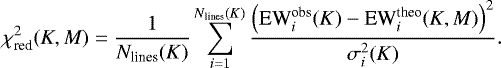
All the following calculations/visualizations have been performed with a custom IDL script written by the authors. Without going into too much detail, for each of our objects K we calculate, for each of the considered elements C, N, and O, the (reduced) χ2 for all models M ∈ MK of our central grid (described by Teff, log g and log Q from Holgado et al. (2018), and a variety of specific abundances and vmic values),
 (2)
(2)
Nlines(K) is the number of useful lines for the considered object K, and σi the uncertainty of the equivalent width for line i. Taken at face value, this expression would be simply the standard definition of a  , if σi were a (normally distributed) Gaussian measurement error. However, to account for potential and actual problems in the theoretical spectra to reproduce certain lines (particularly N III 4634/4640/4641, C III 4647/4650/4651, and C III 5696, see Sect. 3.3), we used a method in analogy to the one described by Holgado et al. (2018, Appendix A). This method accounts for an (implicit) weighting factor for “problematic” lines that cannot be reproduced by the spectrum synthesis within the observed errors (see Eqs. (A.2) and (A.3), and the corresponding text of Holgado et al. 2018). In our case,
![\begin{equation*}\sigma_i(K) = \max\left[{\sigma_{i}^{\textrm{obs}}}(K), {\sigma_{i}^{\textrm{fit}}}(\mbox{best-fitting model}\in{M_{K}})\right], \end{equation*}](/articles/aa/full_html/2019/03/aa33738-18/aa33738-18-eq5.png) (3)
(3)
where  is the uncertainty of the measured
  as derived from our equivalent width measurements (Sect. 4.1), and
 (4)
(4)
among all models M ∈ MK. The “best-fitting model” (i.e., the one with the lowest  ) needs to be determined from an iterative procedure, as described by Holgado et al. (2018). In this way, we renormalize the individual contributionof line i (to a value of unity for the best-fitting model, and to a larger or smaller value for the others) if the corresponding equivalent width cannot be reproduced by the best-fitting model within the observational errors. The other way round, this line becomes implicitly weighted by a factor
![\begin{equation*}w_i=\min\left[ 1, \frac{({\sigma_{i}^{\textrm{obs}}})^2} {\left(\textrm{EW}_{i}^{\textrm{obs}}-\textrm{EW}_{i}^{\textrm{theo}}(\mbox{best-fitting model})\right)^2} \right], \end{equation*}](/articles/aa/full_html/2019/03/aa33738-18/aa33738-18-eq10.png) (5)
(5)

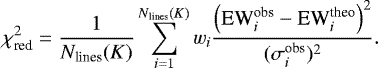
For most lines and stars, our simulations give theoretical EW’s that are well within the observational errors (with an adopted minimum of 10%), that is, wi = 1, but in “bad” cases, wi can reach values of 0.25 or even less9.
The above procedure gives a fair “compromise solution”, by limiting, after convergence and for the best-fitting model, the impact of non-reproducible lines to a value of unity in the sum defining χ2 (Eq. (2)). If we would not apply such a weighting, the finally derived χ2 would be dominated by non-reproduced lines, due to their large deviation compared to the observational uncertainty.
Having calculated the reduced  for all theoretical models MK (i.e., for all abundances and vmic-values present in the grid), and independently for C, N, and O, the resulting abundance corresponds to the model with the lowest
  ,
,
![\begin{equation*} {\chi_{\textrm{red,min}}^{2}}(K) = \min_{M\in{M_{K}}}\left[{\chi_{\textrm{red}}^{2}}(K,M) \right], \end{equation*}](/articles/aa/full_html/2019/03/aa33738-18/aa33738-18-eq15.png) (7)
(7)
and the errors on the abundances and microturbulences can be derived from analyzing the projected (roughly corresponding to the marginalized)  distribution, with n-σ errors corresponding to the location where
 (8)
(8)
We note that the resulting error estimates would be strictly valid only for a large number of terms in the χ2 sum (for a more rigorous study of the properties of a weighted sum of chi squares, see Feiveson & Delaney 1968). For our purpose, however, the limiting expression is sufficient, given the fact that, as we will discuss below, the impact of uncertain stellar parameters is usually of similar size or even larger.
Our IDL script not only provides the final values plus (asymmetric) errors for abundances and vmic, but also displays the corresponding χ2 iso-contours in the abundance–vmic plane10, together with the projected distributions. Moreover, it tabulates also those lines where the weighting factor is lower than 0.5, to check for problematic lines. Examples for the described analysis are given in Appendix B.
From the above description, it should be clear that we determined the best-fitting vmic-values individually, that is, per element. Reassuringly, for almost all objects these values are identical or quite similar for C, N, and O, so that in Table 3 we quote only one value per object. One might argue that different vmic-values would be “allowed” if vmic varies with height (which is most likely true), but then all those lines from different elements/ions that have the same formation depth should display the same vmic. Since in our approach weinvestigate different lines from different ions of one atomic species, such a variation should be present already within one such species. Thus, the derived vmic-values are certainlyonly representative averages, and their similarity within C, N, and O tells that the overall formation depths are not too different (or that vmic varies only mildly, if at all, with depth).
Subsequent to the χ2 minimization, we compared the synthetic profiles from the best-fitting model with observations, to check the overall representation of the line profiles, andto check for the problematic lines already identified within the script. This step also allows to constrain the macroturbulence vmac (see corresponding entry in Table 1), by varying – if necessary – this quantity until the line-shape is matched. This is possible here, since we have reliable values for v sin i and vrad (from Holgado et al. 2018) already at our disposal: if the observed and theoretical EW’s are identical/similar (as true for the majority of analyzed lines in the best-fitting model), the solution is unique, as long as a variation of vmac preserves the equivalent width. Examples for the agreement between observed and theoretical line profiles are provided in Appendix C.
In the last step of our analysis, we investigated the errors due to uncertain stellar parameters (we remind the reader that we have here concentrated on Teff and log g, leaving log Q at the value suggested by Holgado et al. 2018). In this step, we repeat the above procedure, now using the two additional model grids with either Teff and log g increased or decreased. For most objects, this indeed results in different abundances (vmic mostly remains at the original value), where typically the derived abundances for the hotter and higher gravity models turned out to be larger by 0.1 dex, and lower by 0.1 dex for the cooler and lower gravity models. The corresponding (intrinsic) uncertainties were found to be quite similar to the values derived for the original grid. Thus, we approximate the total error from both sources of error – (1) from the χ2 distribution, and (2) from uncertain stellar parameters – as the direct sum of both quantities, where for error (1) we used the corresponding 1-σ error. We stress that constrasted to error (1) this total error cannot be considered as a 1-σ error, but corresponds to a typical error range valid for the considered variation of stellar parameters. A statistical error interpretable as standard deviation could be only obtained if many more models were calculated.
In rare cases (for instance, star #1), the contribution of error (2) is negligible, and for a few other cases both the hotter and the cooler models produce changes in the same direction, so that the total error becomes strongly asymmetric (example is carbon in star #13). For a comparison of the total errors and error (1) alone, see Fig. 1.
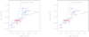 |
Fig. 1. Relation between nitrogen-to-carbon and nitrogen-to-oxygen ratios. Left panel: our results with (approximate) errors when including the uncertainties in Teff and log g. Right panel: only those uncertainties that arise from our method when relying on the Teff and log g values provided by Holgado et al. (2018; see Sect. 5.1). “Hot” and “cold” dwarfs are denoted by blue and red squares, and hot and cold supergiants/bright giants by cyan and magenta asterisks. For our division between hot and cold objects, and the correspondence between number and object, see Table 3. The solid lines represent the theoretical limits for the early phases of the CNO cycle (less massive stars), and for the conversion of O to N after afast establishment of CN equilibrium (most massive stars). Both curves adopt the initial abundances from the Geneva models (Ekström et al. 2012, see Sect. 6.1 and Table 4). |
5. Results
5.1. Basic considerations
Our final sample comprises 18 presumably single O-type stars with spectral types in the range O9.7–O4, including ten dwarfs and eight supergiants/bright giants. Our sample is biased by our selection of objects with comparatively low v sin i, and by most of the stars being in a different stage of evolution (see Sect. 6.2): if at all, our sample comprises only one object per spectral type, which might be atypical.
Regarding our equivalent width analysis, microturbulence plays a major role due to its impact on EW, and consequently on the derived chemical abundance. Each profile/equivalent width was calculated for multiple vmic, and by our χ2 minimization we searched for the best compromise for all the lines of the different elements. Table 3 displays the final estimated vmic value for each star, collecting the information from C, N, and O.
Lines for which it was not possible to measure the observed EW due to their weakness or absence, and lines with atypical shape due to blends were discarded from our statistical analysis, though in all cases we tried to keep the highest number of lines possible. Table 3 displays the number of lines used to obtain the abundance of each atom in our targets. Considering all measurable lines (partly with different weights determined by our minimization algorithm, see Sect. 4.3), we obtained our final estimates for the individual abundances, also displayed in Table 3. Hereafter, we use the notation ϵX = log10(NX∕NH) + 12, where NX is the particle number density of element X (here: C, N, O), and NH is the number density of hydrogen.
The corresponding (logarithmic) uncertainties (first error entry) range between 0.1 and 0.2 dex, and result from the properties of the χ2 distribution when assuming that the stellar parameters are perfectly known. Accounting also for corresponding errors, the second entry (usually larger than the first one) gives the approximate total error budget.
These quite large uncertainties in the abundances are typical for massive, early-type stars, since for these objects it is more difficult to obtain precise constraints on the stellar parameters, due to the presence of (inhomogeneous) winds and the NLTE conditions, contrasted to the conditions in late-type stars, which moreover display significantly more optical lines and rotate slower. Finally, when evaluating the abundance errors, many investigations do not account for the propagation of errors associated with the uncertainty in the stellar parameters.
Table 3 is divided into dwarfs (upper part) and supergiants/bright giants (lower part), with a subdivision into hotter and cooler objects denoted by different colors in the figures in the following sections.
5.2. General comments
Though most of our diagnostic lines could be consistently reproduced, both with respect to EW and line profile, there are also some lines which would indicate different abundances than the majority of the others. The triplet N III 4634/4640/4641 (in emission for hotter objects) is an example well documented by Rivero González et al. (2012a) and Grin et al. (2017). From our results, we confirm their findings, at least for the cooler stars of our sample (Fig. C.1), while for most hotter objects we have not found particular difficulties, and were able to fit the corresponding emission line complex either well or at least qualitatively (Figs. C.2 and C.3). Presumably, the former problem relates to an inaccurate description (in FASTWIND) of the population of the upper levels of these transitions, which depend, in the “cooler” domain of our sample, on the interaction between two overlapping nitrogen and oxygen resonance lines in the EUV (see Rivero González et al. 2011). In terms of our fitting procedure, the N III triplet lines receive a low weight when they cannot be reproduced.
We also suspect (again mostly for the cooler objects) that O III 5592 tends to imply higher oxygen abundances compared to its peers. This would be even more dangerous than in the former case, since this line, due to its strength, is often used as main abundance indicator (e.g., Martins et al. (2015b), 2017). We will come back to this problem in Sect. 5.5.
Finally, also C III 4647/4650/4651 and C III 5696 (see previous sections) often cannot be satisfactorily reproduced (here, both in the cooler and hotter domain), and often receive a low weight as well.
At the end of this section, we note that Table 1 compares the values of vmac as derived by Holgado et al. (2018) and us. Basically, both works used different methods: regarding vmac, Holgado et al. (2018) mostly concentrated on O III 5592, whereas in our work we adapted, if necessary11, vmac to fit the shape of all visible CNO lines as well as possible (see Sect. 4.3). Overall, both results are quite consistent, and the mean deviation is vmac (ours)− vmac (Holgado et al. 2018) = −5.9 km s−1, with a dispersion of ± 7.0 km s−1. The fact that our values are systematically lower than those from Holgado et al. (2018; at least for the dwarfs; for the supergiants, the values are basically equal) might be partly explained by the notion (already mentioned in Sect. 3.1) that Holgado et al. (2018) assumed a delta-function for the intrinsic profile (see also Fig. 5 of Simón-Díaz & Herrero 2014); in contrast, our theoretical profiles already include a thermal plus microturbulent broadening, potentially giving rise to lower vmac when comparing to observations.
5.3. Microturbulence
Before concentrating on the results for the individual abundances, we briefly discuss our findings for the vmic values (see Table 312). Interestingly, the majority of the values are consistent with those estimated by Holgado et al. (2018) from a pure H/He analysis, though our results show a clearer trend: except for one case, all supergiants display (in CNO) a vmic = 15–20 km s−1, where the larger value only appears for the two hottest objects. For the dwarfs, a clear increase with temperature, from 5 to 20 km s−1, seems to be present, where, again, only the (three) hottest objects reach the maximum value. We note here that since both 5 and 20 km s−1 are located at the borders of our grids, these values must be considered as upper or lower limits only, with the exception of star #10. In this case, the quoted vmic = 20 km s−1 value is not a lower limit but a typical value, derived from a compromise between our results for C, N, and O.
The analysis of much larger samples than the present one might allow for tighter constraints on this quantity (as a by-product of the CNO analysis), and might provide useful insights into the question whether there is a physical interpretation for this quantity (in the photosphere), and whether indeed it might be related to sub-surface convection as suggested by Cantiello et al. (2009).
5.4. A consistency check – mixing-sensitive ratios
Due to their sensitivity to mixing, the surface nitrogen-to-carbon (N/C) and nitrogen-to-oxygen (N/O) ratios allow us to obtain constraints on the evolutionary stage of a star, particularly since the CN cycle and the ON loop might not happen simultaneously. In the most massive stars, for example, the conversion of C to N occurs on very fast time scales, and these objects spend most of their subsequent life in converting O to N (e.g., Maeder 2009; Maeder et al. 2014). Thus, it is also important to study the individual C, N, and O abundances in the light of the evolutionary tracks, and to identify any atypical over- or underabundances.
Before concentrating on these issues in Sect. 6, at first we will investigate the (N/C) ratios as a function of (N/O). This behavior is tightly constrained, independent of specific evolutionary tracks, and thus allows us to check the reliability of our data.
Basically, two limiting scenarios can be formulated analytically (see Przybilla et al. 2010 and Maeder et al. 2014). In the case of the most massive stars (≳40 M⊙), the CN equilibrium is quickly established through the CN cycle (12 C →14N), and thereafter the number of carbon atoms can be adopted as constant. Then (as detailed by Maeder et al. 2014),
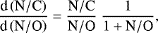 (9)
(9)
and integration (with C = constant) yields13
 (10)
(10)
The second scenario applies to lower mass stars (though still massive), for which one may assume that during the first phase of the CNO cycle (the CN sub-cycle) 16O remains constant while 12C is converted to 14N. Following again Przybilla et al. (2010) and Maeder et al. (2014),
 (11)
(11)
which has a solution symmetric to Eq. (10),
 (12)
(12)
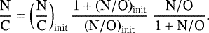
To express (N/C) as a function of (N/O), this can be rewritten as
 (13)
(13)
Both limits, Eqs. (10) and (12), are represented by solid black lines in Fig. 1, and actual objects should be located in the area between these two lines. We stress that the actual location of this area depends on the initial composition, where in Fig. 1 we have used the values adopted by the Geneva models (Ekström et al. 2012, see Sect. 6.1 and Table 4), which are close to the solar ones. We note that a similar comparison has been provided by Martins et al. (2015b, their Fig. 5), also for a sample of Galactic O-type stars (see next section).
The right panel of this figure displays our results with error bars from considering only the uncertainties within our statistical analysis, keeping Teff and log g at the values provided by Holgado et al. (2018) The left panel accounts for a more complete error propagation, considering also the typical uncertainties of the former parameters. This panel shows clearly the importance of including these uncertainties (see also, e.g., Villamariz et al. 2002; Hunter et al. 2007).
Inspecting now the “observed” surface ratios, we see that most of the dwarfs are indeed located at or close to the beginning of the limiting curves, as should be expected (initial phase of their chemical evolution at the surface), though the values also indicate that the cooler dwarfs might suffer from too low values of oxygen. We will return to this problem in the next section. HD 96715 (#10), our hottest dwarf, is separated from its peers and close (at least with respectto its central value) to the early CNO cycle limit which means that most probably this star still displays products of the CN sub-cycle, though already from a later phase with depleted C together with a high N abundance. Cases in analogy to HD 96715 were discussed by Rivero González et al. (2012a), who also found a few, highly nitrogen enriched early O-type dwarfs, within a sample of LMC O-stars. Taken at face value, the location of this object seems to be reasonable. In Sect. 6.2, however, we will see that this object has quite a large mass (from its position in the HRD), and should thus be located closer to the lower limiting curve. We stress, however, that part of this peculiarity might vanish when accounting for the considerable error bars.
The supergiants are mainly located close to the lower limit (at or close to CN equilibrium values), with different stages of nitrogen enrichment. Since all of them turn out to be quite massive (Sect. 6.2 and Table 5), this behavior is as expected. At first glance, the position of HD 152249 (#13) is quite intriguing, and in the next section we provide further details on this object. Anyhow, the large error bars also suggest that the actual position of this star is compatible with a (close to) solar initial composition.
In summary, except for the cooler dwarfs and few specific objects, the derived abundance ratios of our targets are consistent with the theoretical expectations related to their classification. Further constraints on the reliability of our data will be provided in the next section.
5.5. Comparison with previous studies
Three objects of our present sample were already studied (with respect to ϵC) in our previous work (Carneiro et al. 2018), to test the reliability of our carbon model atom. Back then we used a simple by-eye fitting method, and reassuringly our new results (based on a more objective method) are fairly similar (and overlap within the error bars) for all three objects. In particular, for HD 36512 (#1) and HD 303311 (#9), our previously derived carbon abundances were 0.1 dex higher, while for HD 169582 (#19) we found identical values (significantly constrained by the absence or weakness of specific C III lines, cf. Carneiro et al. 2018, their Fig. 10).
Half of our sample overlaps with objects investigated by Martins et al. (2015b, 2017), both by means of a complete CNO analysis. Moreover, for five of our objects, we can also compare with the nitrogen abundances derived by Markova et al. (2018). We refrain from a detailed comparison of stellar parameters, and only note that there is a reasonable agreement14. In the following, we focus on a comparison of the derived abundances.
Figure 2 displays the differences between the logarithmic C, N, and O abundances obtained in the present work and those from Martins et al. (2015b), for the stars common to both samples (IDs on the x-axis), #1, #2, #3, #4, #6, #13, #15, #17, and #18 (see Table 1). Since the target IDs follow the spectroscopic designation (with dwarfs below #10, and supergiants/bright giants above), this figure enables the identification of potential trends in the differences: though in most cases the results coincide within the error bars, our values for the C and O abundances of the cooler dwarfs are generally lower, on average by 0.17 and 0.32 dex, respectively. Moreover, our C abundances for the supergiants are generally larger, by a mean of 0.18 dex. For other elements/objects, no clear pattern can be identified.
Large differences in nitrogen (middle panel) are found for HD 152249 (#13) and HD 151515 (#18). Though it is difficult to find the actual reason for this disagreement, we note that star #13 is an OC-star, characterized (among other features) by having little nitrogen enrichment. Indeed, our abundance is much closer to solar than the value obtained by Martins et al. (2015b; see also Martins et al. 2016 for a study of the four presently known Galactic OC-stars).
On the other hand, our nitrogen abundance for star #18 basically relies on N III (and one weak line of N IV), and has quite a large uncertainty.
In this panel, we also compare (via black dots) our nitrogen abundances with the values estimated by Markova et al. (2018). These authors obtained ϵN through a by eye fit of the nitrogen line profiles (synthesized also by FASTWIND, using the same model atom), giving a larger weight to those lines that are stronger and not affected by stellar winds. The comparison was possible for stars #3, #5, #7, #13, and #19. Markova et al. (2018) did not quote individual uncertainties, but provide a typical error of ±0.2 dex, which has been considered in the black error bars. The values derived by Markova et al. (2018) are consistently higher than ours (on average by 0.19 dex), both for the three dwarfs and the two supergiants, but still agree within the 1-σ range, where HD 97848 (#5) just marginally touches this range, due to a quite low positive error from our side. Their nitrogen abundance for HD 152249 (#13), the OC-star, is also closer to the solar value than that of Martins et al. (2015b), but still 0.25 dex larger than ours. This example instructively quantifies typical deviations in derived abundances from hot stars even when using identical synthesis tools, but different methods15 to infer the parameters and abundances.
As already pointed out, our oxygen abundances for the cooler dwarfs are considerably lower than those derived by Martins et al. (2015b), while for the other objects there is no clear trend. Here also, however, two objects show considerably less oxygen. There mightbe (at least) two reasons for this discordance: (i) as mentioned in Sect. 3.3, our present oxygen model atom lacks a detailed description for specific transitions, and thus might lead to an inaccurate description of certain levelpopulations. (ii) Martins et al. (2015b; in both papers) provide an extensive list of lines used for their oxygen analysis, but most of these refer to O II, and only O III 5592 is used for O III. Thus, at least for higher Teff and/or higher v sin i, O III 5592 is the only diagnostic oxygen line in their analyses. From our own experience accumulated in the present study, this line almost always indicates larger oxygen abundances than the other O III lines used by us in addition to O III 5592 when possible (see Table 2). Since our diagnostic method always searches for a “compromise solution”, this leads tolower derived oxygen abundances. We have checked that using O III 5592 exclusively would result in ϵO values rather close to those derived by Martins et al. (2015b), but presently we have no reason to exclude the other lines.
From the comparisons performed in the previous and this section, we conclude that our carbon and nitrogen abundances should be, overall and within the error bars, reliable, and significant differences to the studies by Martins et al. (2015b) are present only in the N abundance of two stars.
For the cooler dwarfs, the comparison with the theoretical limits of CNO burning points toward too low oxygen abundances, and the discrepancies with Martins et al. (2015b) are systematic. Moreover, it would be difficult to explain why our cooler dwarf sample should display (on average) considerably less oxygen than B-stars in the solar neighborhood (ϵO ~ 8.76, Przybilla et al. 2008) or at least B-stars in the young open cluster NGC 6611 (ϵO ~ 8.55). We note here that problems with FASTWIND itself are unlikely, since Simón-Díaz (2010) analyzed 16 B-type stars in the Ori OB1 association with this code, and found highly homogeneous oxygen abundances, in good agreement with the quoted work by Przybilla et al. (2008). Unfortunately, their oxygen model atom was tailored for early B-type dwarfs, and could not be used for the analyses of the hotter sample investigated here.
Since the identified, systematic discrepancies in the oxygen abundance are specific for our cooler dwarfs (dense atmospheres), it is quite possible that this problem – if there is one – is indeed rooted in our current model atom, since (i) problematic ionization cross sections can lead to an erroneous ionization balance, which might explain our almost perfect fits for O II (Fig. C.1), and (ii) imperfect collisional strengths have a major effect particularly at high densities and comparatively cool temperatures. Although the situation for the other objects is more promising, both in terms of the location of these objects in Fig. 1, and in comparison to Martins et al. (2015b), the validity of our oxygen analysis as a whole needs to be clarified in forthcoming work. We stress, however, that our results do reproduce the observed oxygen lines – admittedly, O III 5592 to a lesser extent – but we advise considering our oxygen results with caution until further evidence.
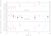 |
Fig. 2. Differences between the logarithmic chemical abundances obtained in the present work and those from Martins et al. (2015b, 2017; colored symbols as in Fig. 1) and Markova et al. (2018; nitrogen only, black circles). Errors of own data include typical uncertainties in stellar parameters. |
6. Comparison with evolutionary calculations
6.1. Stellar evolutionary models
In the following, we will compare the outcome of our study with theoretical predictions. In particular, we will compare with two well-known evolutionary grids for single massive stars, namely the tracks from Ekström et al. (2012), henceforth referred to as Geneva tracks, and from Brott et al. (2011), referred to as the Bonn models. Details on the differences between these two investigations can be found, e.g., in Keszthelyi et al. (2017) and Markova et al. (2018). Both grids include rotation (adopting different descriptions for angular momentum transport and mixing), with a variety of initial velocities (Bonn grid), or one specific initial rotation rate, corresponding to 40% of critical rotation (Geneva). Grids without rotation are available as well.
The Bonn tracks additionally adopt magnetic fields, which have been accounted for in the angular momentum transport, but not for mixing. For our concern, important distinctions between both tracks are initial metallicities and the core overshooting parameter.
Table 4 compares the different initial CNO compositions used in each of the tracks, together with the solar abundances from Asplund et al. (2009), which serve as central values for our atmospheric model grids. While the chosen initial conditions from the Geneva grid are quite similar to the solar ones (for details, see Ekström et al. 2012), the values adopted in the Bonn tracks have been tailored to represent the conditions in the young open cluster NGC 661116, basically using data from early B-type stars and H II regions located in this cluster (for details, see Brott et al. 2011).
The initial metallicity has a moderate effect on the individual abundances and abundance ratios when evolving with time (e.g., Brott et al. 2011, Grin et al. 2017). Since the mixing efficiency parameter is larger in the Bonn tracks (at least for the mass range of our sample – see, e.g., the comparisons provided by Keszthelyi et al. 2017), also the time-scales of the chemical evolution at the surface differ in both models. On the other hand, overshooting plays a major role for the duration of the main sequence (e.g., Maeder 1976; Chiosi 1986), and a larger overshooting (Bonn models) results in a more extended main sequence phase (reaching into the B-supergiant regime), compared to the Geneva tracks.
Initial values of CNO abundances adopted in the evolutionary grids referred to in this work, and corresponding solar values from Asplund et al. (2009).
6.2. Evolutionary stages
Already with our inspection of the abundance ratios (Sect. 5.4 and Fig. 1), we obtained some insights intothe evolutionary phases of our targets. However, the correlation between evolutionary stage and nucleosynthesis evolution is complex, due to the many processes to be considered. Stars of different masses experience different phases of the CNO cycle at different times, where carbon reaches equilibrium considerably faster in more massive stars (e.g., Maeder 2009; Maeder et al. 2014). Before proceeding with our investigation of the abundance evolution, we thereforebriefly constrain the evolutionary stages of our sample stars by comparing with suitable diagrams, which then allows us to cross-check with our previous and following conclusions obtained from the abundance analysis. Since we have used the stellar parameters from Holgado et al. (2018), and since part of our sample overlaps with the samples from Martins et al. (2015b, 2017) and Markova et al. (2018), corresponding conclusions on masses etc. can be already found in these studies.
To avoid any uncertainty induced by uncertain distances (in the same spirit as Holgado et al. 2018), we consider only those diagrams/variables that are independent of stellar radius, and only depend on quantities derived by means of quantitative spectroscopy.
To this end, we examined the location of our sample stars in the log g–Teff (Kiel) diagram, and, because of the clearer separation of the theoretical tracks, in the spectroscopic HR diagram (sHRD, Langer & Kudritzki 2014). The latter uses as ordinate the variable  , where
 (14)
(14)
and gtrue is the (spectroscopic) gravity, corrected for centrifugal acceleration17. Since  , it is also proportional to the Eddington Γe for electron scattering, which we have additionally indicated on the right ordinate of the corresponding figures.
Though our sample consists of stars with v sin i < 100 km s−1, all following comparisons are based on the rotating Geneva and Bonn evolutionary tracks, which are represented in the next figures by black and red lines, respectively, with an initial rotation velocity of 40% (or close to this value) of the critical speed. For the mass range considered (20–60 M⊙), this corresponds to ~270 to 350 km s−1. We note that the Geneva tracks do not include a track for 30 M⊙, but for 32 M⊙.
The reasons for comparing with models of such relatively high initial rotation rates are as follows: the low v sin i values of our sample stars refer to the current evolutionary stage, and at least for the supergiants a sizeable rotational braking due to angular momentum loss is expected. Thus, some sample stars should have indeed started their lives with considerable rotation. Moreover, a significant fraction of the analyzed stars display nitrogen enrichment, which, in the single star scenario, can be only explained by rotational mixing, again requiring a considerable initial vrot. Thus, we need to compare with rotating models, since non-rotating models would preserve the surface abundances during the main sequence, prohibiting any further conclusions. At least at the time of finalizing this study, however, the only public available rotating models from the Geneva group were those with an initial vrot = 0.4vcrit, and for reasons of consistency, we choose a similar value for the Bonn models. Moderate differences between the main sequence HRD-tracks of rotating and non-rotating stars can be seen only for higher mass stars (which indeed might require the consideration of tracks including rotation, see above), whereas for the majority of our sample stars their positions in the HRD (contrasted to their surface abundances) are hardly affected by the inclusion of rotation, and we do not aim at a precise mass determination anyhow. In our further discussion, we keep these problems in mind.
Concentrating now on the evolutionary phases, our sample stars populate the considered mass range, as evident from the left (Kiel diagram) and the right panel (sHRD) of Fig. 3, with the majority of dwarfs being in the early main sequence phase. The early supergiants are mostly located in the intermediate phase, around 40 M⊙, while the cooler supergiants (together with the hot supergiant HD 225160 (#16)) are either in the late MS phase (Bonn tracks, with larger overshooting), or already at or close to the TAMS (Geneva tracks). Star #12 is the most evolved star, which according to the Geneva tracks might be already in the hydrogen shell-burning phase.
From Figs. 3 and 4 (discussed below), a clear lack of massive stars close to the ZAMS is obvious. Though this might be pure coincidence due to our small sample, such findings have been reported already previously, for different samples (e.g., Herrero et al. 1992, Repolust et al. 2004, Martins et al. 2005, Simón-Díaz et al. 2014). More recently, and for much larger samples, Sabín-Sanjulián et al. (2017; with respect to the VFTS, Evans et al. 2011) and Holgado et al. (2018; with respect to the Galactic O-type standards) identified the same problem18.
In addition to our present lack of knowledge of how pre-main-sequence stars initiate their evolution on the main-sequence (e.g, Bernasconi & Maeder 1996, Behrend & Maeder 2001, Haemmerlé et al. 2016), very young massive stars could still be enshrouded by the dust from their birth cocoon, which would hide these targets from optical observations (e.g, Garmany et al. 1982, Herrero et al. 2007, Castro et al. 2014), and might explain the observed deficit of massive stars close to the ZAMS. A more detailed discussion on this topic will be presented in a forthcoming paper of the IACOB series (Holgado et al., in prep.).
Regarding the implied stellar masses, both tracks basically agree for all dwarfs, with the exception of HD 97848 (#5: 32 M⊙ from the Geneva, and40 M⊙ from the Bonn tracks). For the supergiants, however, there are clear differences. From the Geneva tracks, our most evolved stars range from 32 to 40 M⊙, while from the Bonn tracks they range from 40 to ~65 M⊙. In particular, for HD 195592 (#12) the Geneva tracks imply a mass of ~40 M⊙, contrasted with ~65 M⊙ from the Bonn models. These disagreements presumably relate to the different treatment of angular momentum transport and mixing (in particular, the effects from mean molecular weight barriers), which results, in the Geneva models, in higher luminosities and consequently higher mass loss. Accounting for the higher luminosities and the increased mass loss, both the actual and the initial masses of more evolved objects are lower than in the Bonn models. For more details on these discrepancies, we refer to Markova et al. (2018).
Concentrating now on the sHR diagram (right panel of Fig. 3), which provides a distance independent luminosity-to-mass ratio19, we note that  increases in parallel with the ID numbers of our dwarfs, and two of them (HD 93222 (#7), and HD 96715 (#10)) belong to the stars with the highest luminosity-to-mass ratio, headed by HD 195592 (#12).
For the sake of clarity, we display  also as a function of log g in Fig. 4, which shows an even better distinction between the tracks for the individual masses, and provides an impression of the different location of the TAMS in the alternative evolutionary models. From this figure, we can divide our sample in two regimes, divided around log g ~ 3.65. On the left side, we find the stars with higher gravities and mostly lower luminosities (dwarfs). In this regime, the atmospheres are denser, and the ionization balance is shifted toward lower ionization stages. Since these have more lines in the optical (which improves the abundance analysis), the stars in this regime are also the stars with the most precise results, in other words, with the smallest uncertainty ranges (see Table 3).
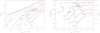 |
Fig. 3. Left panel: Kiel diagram (log g vs. Teff) for our sample stars. Overplotted are the rotating Geneva (Ekström et al. 2012; black) and Bonn (Brott et al. 2011; red) tracks for the mass range 20–60 M⊙, with initial rotation velocities of 40% of their critical speed. Right panel: corresponding spectroscopy HR diagram (sHRD, see text), with both ordinate-axes proportional to L∕M. The Eddington Γe has been calculated with solar Helium content, assumed to be completely ionized. Symbols in both panels as in Fig. 1. |
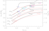 |
Fig. 4. Modified sHRD, with abscissa log g (instead of Teff), providing a clearer separation between the tracks. Two distinct gravity regimes populated by our sample stars become obvious (see text). |
6.3. CNO evolution
The different evolutionary stages occupied by our sample provide us with a well suited laboratory for the analysis of general trends (and outliers). The division into two regimes, particularly seen in Fig. 4, should be also present when comparing ϵC vs. ϵN as done in Fig. 5. Lower mass dwarfs should still show the products of the CN cycle (and in most cases, from its early phases), with carbon and nitrogen surface abundances not too different from their initial values (which might vary as a function of environment, see Table 4), while the supergiants and the more massive dwarfs should become significantly nitrogen enriched and carbon depleted.
Even though we already discussed the behavior of mixing-sensitive abundance ratios in Sect. 5.4, there are indeed good reasons to study at first the ϵC vs. ϵN relation, without relying on the oxygen abundance: (i) at least for the cooler dwarfs, the ϵO values derived in the present work need to be rechecked (potential deficiencies within our oxygen model atom, see Sect. 5.5). (ii) At least from intermediate O-types on, the oxygen abundance is the most difficult to determine among the three elements C/N/O, due to the restricted number of ions (only O III) and corresponding lines in the optical, and the potentially peculiar behavior of O III 5592 (Sect. 5.2).
Together with the relation of ϵC vs. ϵN for our sample stars, Fig. 5 displays the evolution of these surface abundances as predicted by the Geneva (black) and Bonn (red lines) tracks (again with  ). Except for the different initial conditions, the predicted relations are quite similar, with only slightly diverging curves for the 60 M⊙ tracks, though the evolution of the individual abundances as a function of other parameters (evolutionary time or Teff) is quite different, as we will see in Fig. 6. This clearly shows that the evolution of the surface abundance ratios is mainly triggered by nucleosynthesis when mixing is efficient.
In Fig. 5, the 20 M⊙ tracks exemplify the lower range of abundance variation predicted for all stars with less than 40 M⊙. For example, for the 20 M⊙ Geneva track, ϵC decreases from 8.39 to ~8.12, and ϵN increases from 7.78 to ~8.43 (see below).
In general, our sample follows, within the error bars, the trend suggested by the tracks, with the majority of the stars in between the two curves, which might be indicative for the potential variation of (initial) CN abundances in the solar surroundings.
Concentrating at first on nitrogen, the majority of the dwarfs have ϵN values much closer to solar20 than the supergiants, as expected. Two dwarfs (#8 and #10) and one supergiant (#13) are an exception to this behavior. Regarding the dwarfs, HD 12993 (#8) has been classified with the suffix “Nstr”21, implying an increased nitrogen and decreased C abundance (as derived here). HD 96715 (#10), our hottest and most massive dwarf, and already referred to in Sect. 5.4, displays even more ϵN and less ϵC, indicating the products of a rapid CN cycle, which, following Fig. 1, have not yet reached equilibrium though. The OC-supergiant HD 152249 (#13) has already been mentioned in Sect. 5.5.
Turning now to carbon, here also most of the dwarfs have ϵC close to initial values. However, the predicted depletion is not (or at least not clearly) visible for the supergiants, which display a range of carbon abundances comparable to the dwarfs.
Accounting for the uncertainties, one might argue that also our hotter supergiants are still compatible with the Geneva tracks, except maybe for #17 (HD 171589), which shows the largest difference to the predictions (all hotter supergiants need to be compared with the 40 M⊙ track, see Table 5). We remind the reader that regarding the abundance ratios (Fig. 1), #17 “fits” perfectly, which emphasizes the importance of considering the individual abundances as well.
At this point, we stress again the prime role of rotation in defining the position of each target in Fig. 5, and the position of the theoretical tracks. Initial rotational rates lower than 0.4 vcrit will decrease the range of predicted enhancements and depletions (and a very low initial rotation results in a negligible evolution of CNO surface abundances), which might explain the position of our OC-supergiant #13 with v sin i ≈ 70 km s−1 (see also Martins et al. 2016, who suggested the same scenario). Indeed, according to our selection criteria, most of our objects should be in a present state of slow rotation (if, as reasonable, only few of them were observed close to pole-on). Nevertheless, almost all hotter supergiants plus the dwarfs #8 and #10 show a significant abundance evolution, and this would imply that there is a significant loss of angular momentum already before the potential bi-stability braking (Vink et al. 2010) around 25–20 kK. Moreover, at least for those few stars that show a very strong enrichment, there is the chance that they rotate much faster than suggested by their v sin i, and for those stars a higher initial rotation than assumed here might be possible, with consequences for the predicted CNO evolution.
Thus far, our investigations have concentrated on surface-abundance ratios, where, assuming that the mixing-processes are similar for the considered elements, Figs. 1 and 5 mostly reflect the conversion of elements due to the CNO cycle, in dependence of initial composition. Thus, these diagrams are (almost) independent of the actual evolution as a function of time, which is strongly affected by the description of the mixing processes themselves, which in turn depend on the stratification of physical quantities such as internal velocity fields (rotation, turbulence, meridional circulation).
To obtain some insight into this temporal evolution, and to allow a comparison with the alternative approaches from the Geneva and Bonn models, Fig. 6 displays the theoretical predictions (with Teff as a proxy for time) for the individual elements (from top to bottom: C, N, O) and different mass regimes, together with our results. The dotted lines represent the solar abundance for each element, and the dashed and the dashed-dotted lines show the initial abundances of the Geneva (left side panels) and Bonn (right side panels) tracks, respectively.
Comparing both evolutionary tracks in all panels, the consequences of the distinct mixing descriptions used in each of the two sets becomes evident. In the Bonn tracks, all surface abundances reach their equilibrium value considerably faster, due to the larger mixing efficiency used. A consequence of this rapid mixing in the Bonn tracks is that the “hooks" (when the stars begin to contract at the end of the main sequence) are not visible, even if we would extend our Teff range to lower temperatures, while in the Geneva tracks they are clearly visible, independent of mass regime. Moreover, although the predicted maximum depletion of C is similar in the Geneva and Bonn tracks (though the numbers are different because of different initial conditions), the Geneva models predict both a larger maximum N-enrichment and a larger maximum O-depletion22. For more details on the differences in the ϵN evolution, see Markova et al. (2018).
Before further comments are given, we provide in Table 5 some typical mass ranges to be accounted for when comparing our data with the predictions. These ranges in initial mass have been estimated from the sHRDs (Figs. 3 and 4) referring to the Geneva and Bonn tracks with initial rotation ≈ 0.4 vcrit. In addition, this table also displays the initial masses for specific objects discussed in the following. As already mentioned in Sect. 6.2, the initial (and also the actual) masses for more evolved stars as derived from the Bonn tracks are larger than those from the Geneva ones.
Overall, Fig. 6 is compatible with typical expectations. Most dwarfs present abundances close to the initial values, except for HD 12993 (#8) which is our “Nstr” object, and HD 96715 (#10), our hottest and most massive dwarf, both discussed already previously. The supergiants and bright giants show different degrees of chemical evolution, except for HD 152249 (#13, see above), which shows a close to solar abundance also for oxygen, consistent with our hypothesis (and the one by Martins et al. 2016)that this star should have formed with a low rotational speed. A closer look into the specific elements and objects reveals the following:
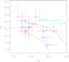 |
Fig. 5. Relation ϵC vs. ϵN in the light of evolutionary tracks. The black and red lines display the corresponding Geneva and Bonn tracks with |
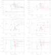 |
Fig. 6. Evolution of C/N/O abundances for different masses (from left to right panels: 60, 40, ~30, 25, and 20 M⊙) as a functionof Teff, as predicted by the rotating Geneva (black lines, left panels) and Bonn tracks (red lines, right panels). The dotted line represents the solar abundance. The dashed and the dash-dotted lines display the initial abundances used in the Geneva andin the Bonn calculations, respectively. Our results (symbols as in Fig. 1) are shown with errors accounting for typical uncertainties in stellar parameters. For initial evolutionary masses of sample stars, see Table 5. |
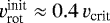
Carbon
While the carbon abundances of the cooler dwarfs and the cooler supergiants (the most evolved objects in this study) are consistent with the predictions from the Geneva tracks, for both the hotter dwarfs (except for #8 and #10) and the hotter supergiants (i.e., higher mass stars at early or intermediate MS-phases), the derived carbon abundance is larger than predicted, that is, the “observed” depletion (if there is any) is lower. The least evolved stars have ϵC similar to the solar abundance, and are thus located closer to the Geneva than to the Bonn tracks. In most cases, our sample shows carbon abundances higher than even the initial values adopted by the Bonn models, though consistent with the initial values from Geneva.
Nitrogen
The cooler dwarfs agree with both tracks, while the hotter ones (again except for #8 and #10) mostly display less nitrogen than predicted. This could be a selection effect, since at least in the LMC there are many early O-dwarfs that show the opposite, see Rivero González et al. (2012b). Comparing with the nine Galactic O-dwarfs earlier than O8 analyzed by Markova et al. (2018), they found a significant nitrogen enrichment in five out of these nine stars, while the other four objects displayed values close to solar. Thus, a final conclusion on typical nitrogen abundances in early O-dwarfs is still not possible, and this discussion needs to be revisited after the analysis of a larger dataset. Anyhow, in combination with the discrepancies found for carbon in this work, our results might indicate that either the carbon depletion sets in later than expected, or, more likely, that these sample stars had a lower initial vrot than considered in the tracks.
Regarding the cooler and hotter supergiants, the agreement is better, particularly compared with the Bonn tracks.
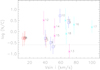 |
Fig. 7. Nitrogen-to-carbon ratio vs. v sin i for our sample stars. The dotted line represents the solar value. |
Oxygen
Here, most of the hotter objects are in fair agreement with the predicted depletion, and also the cooler supergiants follow the predicted trend, though they are more consistent with the Bonn tracks (which start from a lower initial O-abundance). The cooler dwarfs, however, display too little oxygen, compared with both tracks (Minit ≈ 20–30 M⊙), again indicating problems with the abundances as derived for these objects (Sect. 5.5). Taken together, it is quite likely that the deficits in our oxygen analysis mostly concern the cooler O-dwarf domain, while for the rest the analysis appears to deliver reasonable results.
We end this discussion by pointing out that our two hottest stars within the dwarfs and supergiants, #10 and #19, are in very good agreement with the Geneva tracks, particularly regarding nitrogen and oxygen, though at least the latter two elements are also matched by the Bonn tracks within the errors.
Our final diagram, Fig. 7, displays the mixing-sensitive ratio nitrogen-to-carbon vs. v sin i, and is a variant of the meanwhile well-known “Hunter diagram” (ϵN vs. v sin i, Hunter et al. 2008), where in this variant the surface enrichment of N becomes amplified by the parallel depletion of C. This kind of analysis was recently applied to a set of Galactic giants by Martins et al. (2017), who found no clear trend for their sample.
For the further discussion, two remarks might be necessary: (i) since the inclination sin i is unknown, the provided abscissa values are lower limits on the actual rotational speed vrot. (ii) The untypically low (for O-type stars) values of v sin i are a consequence of one of our selection criteria.
Though Fig. 7 implies no obvious trend (such a trend would certainly not have been expected for our sample), it underpins some of our previous conclusions and hypotheses. All cool dwarfs have close to initial surface abundances (whether solar or somewhat different), and this is consistent with any kind of track, be it rotating or not. Three of the five hotter dwarfs also have close to initial abundances, while they should have, if beginning their lives with  , already a well developed N/C ratio. Thus, for these stars it is quite likely that they have started their evolution as slow rotators, in line with the arguments from above. Except for object #18, all hotter supergiants plus the dwarfs #10 and #8 have a well-developed N/C pattern (consistent with or lower than the predictions from the tracks including rotation), which indicates that a considerable braking mechanism (presumably due to the significant mass loss of these objects) must be present already at relativelyearly phases. We refrain here from discussing the theoretical predictions regarding the evolution of vrot, and only refer to Keszthelyi et al. (2017) and Markova et al. (2018) for a closer study on this topic. Similar conclusions (i.e., previous braking) might also be drawn for the cooler supergiants (except for #13 and #15, which most likely started their life with low vrot as well). In both tracks, these objects are still far away from the bi-stability jump with potential bi-stability braking. At least in the Geneva models, however, they are very close to the “hook” (end of the MS phase), where mass-loss and angular momentum might change strongly, due to the significant changes in stellar structure.
7. Summary, conclusions, and future work
In this work, we presented a pilot study on the optical analysis of CNO surface abundances in O-type stars by means of FASTWIND, to be applied to large, statistically significant samples in future investigations (where an analysis by this code is advantageous due to the low computational costs). We have concentrated on targets and observations which should favor a straightforward abundance analysis: high-quality spectra from presumably single Galactic O-stars (which allows us to compare with single-star evolutionary tracks), and low v sin i (to avoid blending).
In particular, we selected a subsample of 18 O-type stars with low v sin i (≤100 km s−1) from the original sample by Holgado et al. (2018), covering ten dwarfs (O4–O9.7) and eight supergiants/bright giants (O6–O9.7), with well determined stellar and wind-strength parameters.
The required model grids for the synthetic spectra have been calculated with the most recent version of FASTWIND, using our well tested model atoms for nitrogen (Rivero González et al. 2011, 2012a) and carbon (Carneiro et al. 2018). For oxygen, we applied the model atom from the WM-basic database (Pauldrach et al. 2001), since thus far we have no “own” oxygen model atom suitable for O-star conditions at our disposal, and since the quoted one has been successfully used in various UV analyses (but not in the optical). When calculating the model grid(s), it turned out that a variation of all three C/N/O-abundances in parallel (per model) is possible, which saves a factor of three computation time and storage.
To derive the CNO abundances, we developed a semi-automatic method accounting for observational and systematic uncertainties, the latter arising due to problems in reproducing specific lines in specific spectral regimes. This method is based on a χ2 -minimization of the (weighted) deviation between observed and theoretical equivalent widths. We have chosen such an equivalent width method to avoid problems related to line broadening (rotation and macroturbulence) which might occur if alternatively fitting the profile shape. The minimization accounts for abundance and microturbulence in parallel, where the latter quantity is important for the final outcome. In our method, we also account for typical uncertainties in the stellar parameters, which introduces a significant contribution to the total error budget.
After analyzing the observed equivalent widths by means of our minimization method, we found that the derived vmic-values are fairly similar for each of the considered elements, and were thus able to provide, per star, a unique value for this quantity. For all supergiants, we obtained values between 15 and ≥ 20 km s−1, whereas the dwarfs displayed a clear trend, with vmic increasing from ≤5 to ≥ 20 km s−1 with spectral type.
After the best-fitting model for each star had been identified, we compared the corresponding line profiles with the observed ones, to check their consistency. This step allowed us to obtain final constraints on vmac, which were found to be similar to the values provided by Holgado et al. (2018) To check the reliability of our analysis, at first we investigated the abundance ratios (N/C) as a function of (N/O), where this relation is tightly constrained from theoretical considerations, independent of actual evolutionary calculations (Przybilla et al. 2010; Maeder et al. 2014). Most of our targets display abundance ratios consistent with the theoretical limits, though already here the OC9 Iab star HD 152249 caught our attention, due to an abundance pattern indicating a very early stage of evolution, though spectroscopically classified as supergiant. More severe deviations (though still within the total errors) were “only” found for the cooler (lower mass) dwarfs within our sample, with too low oxygen abundances compared to the limits.
Part of our sample overlaps with the samples studied by Martins et al. (2015b, 2017) using the CMFGEN code. Except for specific differences that have been discussed in detail, the only major systematic discrepancy refers again to the oxygen abundance of the coolerO-dwarfs, where Martins et al. (2015b) found much larger values than we did. Though part of this discrepancy might be attributed to the behavior of O III 5592 (which in our simulations implied larger abundances than the other O III lines, but was exclusively used by Martins et al. (2015b) for this ion), we suspect that certain deficiencies of the oxygen model atom adopted in our work (see above) might be responsible for this deviation, and caution against using our oxygen results (at least in this spectral domain) until further tests are performed. To this end, we certainly need to develop our own, detailed, and well tested oxygen model atom that is suitable for O-star conditions also in the optical.
Interestingly, five stars of our sample also overlap with the sample investigated by Markova et al. (2018), including a nitrogen analysis, by means of the same code and the same nitrogen model atom. Though the results of both works are compatible within their 1-σ ranges, the central values differ by roughly 0.2 dex, which tells about the accuracy of abundance determinations in hot stars that can be achieved using different methods.
The outcome of our study was compared with two well known evolutionary grids for massive single stars, namely, the rotating ( ) tracks from Ekström et al. (2012; Geneva models), and from Brott et al. (2011; Bonn models). Most important for our concerns are the different overshooting parameters, initial metallicities, and chemical mixing recipes/efficiencies used, due to their impact in prescribing stellar and chemical evolution.
Using the corresponding Kiel and spectroscopic HR diagrams, we obtained an overview on the evolutionary stage of our sample, and on the initial masses, ranging in between 20 and 60 M⊙, where the Bonn tracks imply higher masses for the more evolved objects, compared to the Geneva tracks.
According to the tracks, part of our sample is at the beginning or in an intermediate phase of the MS, while another is at later MS-phases (Bonn) or already close or even beyond the TAMS (Geneva). This division is also found in an ϵC vs. ϵN diagram: lower mass dwarfs still display the products of an early CN cycle, while massive supergiants have become significantly nitrogen enriched. Few objects with particular compositions (for example, the OC-star) have been discussed, but our major finding on more systematic discrepancies regards the hotter supergiants: though well enriched in nitrogen, the corresponding depletion in C remains below the predictions. At this stage, it is difficult to interpret this case, also because we do not know the initial vrot of these objects.
In addition to the ϵC vs. ϵN diagram, we studied the individual C/N/O abundances as a function of Teff (as a proxy of time) in the light of the evolutionary tracks. Many sample stars follow the theoretical expectations, though certain objects are better represented by the Geneva tracks (for instance, our hottest dwarf and supergiant), and others by the Bonn tracks (oxygen in most supergiants). Chances are high that our “oxygen problem” mostly affects the cooler dwarfs, since we found no real discrepancies for the other objects.
Due to the small sample size and our selection criterion regarding v sin i, however, definite conclusions are not yet possible, and many questions remain, such as: is there a fast (Bonn) or slower (Geneva) surface enrichment? What is the “typical” nitrogen content (if there is any) of early O-dwarfs? To answer these and related questions, many more objects per spectral type need to be analyzed. Nevertheless, and in combination with Fig. 7 (N/C as a function of v sin i), some hypotheses could be formulated: three of the five hotter dwarfs are located close to the initial abundances, while they should already have a well developed N/C ratio if their initial vrot was significant. Thus, it is likely that these stars started their evolution as slow rotators. From the derived abundance pattern, the same should be true for the OC-supergiant, in line with an identical hypothesis by Martins et al. (2016). Except for HD 151515, all hotter supergiants plus two hotter dwarfs (HD 12993 and HD 96715) have a well developed N/C pattern, which indicates that an efficient braking mechanism must be present already at relatively early phases (at least if most of these stars were not observed pole-on). Similar conclusions (i.e., previous angular momentum loss, well before the potential bi-stability braking) might also be drawn for two (of four) cooler supergiants (HD 195592 and HD 71304). These notions might provide indirect clues on the “true”23 mass-loss rates of O-stars, assuming that this braking is due to mass loss.
Since in this work we focused on photospheric CNO lines, clumping and X-rays should play a minor role, particularly since the ions that are most influenced by the emission from wind-embedded shocks (C V, N V, O V, and O VI, Carneiro et al. 2016) are basically not included in our present analysis. On the other hand, an optical CNO analysis of the hottest O-stars is significantly hampered by the absence or weakness of corresponding C and O lines (which is the reason that the hottest supergiant in our sample has spectral type O6). For these objects, which are particularly interesting because of their higher masses, a UV analysis is inevitable, and at least then X-ray and clumping effects will need to be accounted for. This is possible already now, thanks to the work by Carneiro et al. (2016) and Sundqvist & Puls (2018), respectively, where the latter included a suitable treatment of porosity effects (also in velocity space) into the FASTWIND code, which might be essential for analyzing abundances from UV lines.
We end our study by concluding that we have developed and tested a method that is big-data-ready, and that FASTWIND is now (almost) well equipped to be useful in the CNO analysis of statistically significant O-star samples, such as the already available VLT-FLAMES, IACOB, and OWN surveys. On the technical side, we still have to work on the oxygen model atom and to perform careful tests, particularly in the cooler O-dwarf domain. On the scientific side, we note that though the analysis of large samples is of prime importance, also the analysis of individual, peculiar objects such as, for example, HD 12993 (the “Nstr” star) and HD 152249 (the OC-star) can lead to considerable progress in our understanding of massive stars, since often one might learn more from the deviations than from the consistencies with current theories.
Acknowledgements
We thank our anonymous referee for very useful comments and suggestions, and appreciate the advice by Dr. Achim Weiss on various topics related to chemical evolution. L.P.C. gratefully acknowledges support from the Brazilian Coordination for the Improvement of Higher Education Personnel (CAPES), under grant 0964-13-1. G.H. and S.S.-D. acknowledgefinancial support from the Spanish Ministry of Economy and Competitiveness (MINECO) through grants AYA2015-68012-C2-1 and Severo Ochoa SEV-2015-0548, and grant ProID2017010115 from the Gobierno de Canarias.
Appendix A: Equivalent width measurements – three typical examples
As discussed in Sect. 4.1, we have developed an interactive algorithm (in IDL) to measure the EW’s of all target lines. Figure A.1 displays three typical examples, namely, for an emission (C III 5696), an absorption (N III 4514), and a blended line (O III 3961), all in the spectrum of HD 46966 (#6). The blue line shows the Gaussian fit (line center of the Gaussian indicated in blue as well), while the red color indicates the wavelength interval used for the fitting procedure and for a direct integration, which was applied to obtain a second, independent measurement. The EW’s resulting from these two methods are usually very similar (less than 5% difference). In the cases displayed in the upper two panels, we measured, for example, for C III 5696, EW (Gaussian) = −62 mÅ vs. EW(direct) = −57 mÅ, and for N III 4514, EW (Gaussian) = 112 mÅ vs. EW(direct) = 117 mÅ. In cases of blended lines (as in the lowermost panel), we fitted the uncontaminated part of the profile by a corresponding Gaussian, and extended the line wings to simulate the blended part. In this case, a direct integration makes no sense. For the displayed example, O III 3961, we found EW(Gaussian) = 141 mÅ. For consistency between the first two and the latter cases, we finally used only the values obtained by the Gaussian fit for all lines. Our procedure to derive an estimate on the corresponding errors is described in Sect. 4.1. We repeat that only N III 4097 was treated differently from the examples shown in Fig. A.1, due to its complete overlap with the Hδ line wing (see also Sect. 4.1).
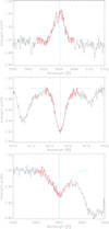 |
Fig. A.1. Examples for equivalent width measurements via Gaussian fits (blue) and direct integration (with respect to the interval indicated in red): C III 5696, N III 4514, and O III 3961, in the spectrum of HD 46966 (#6). |
Appendix B: χ2 minimization – exemplary cases
To determine the optimum set of abundances and microturbulence(s) for each of our objects, we calculated and analyzed the (reduced) χ2 for C, N, and O, via a self written IDL script (see Sect. 4.3). In Figs. B.1–B.3, we exemplify our analysis by means of the plots produced by this script. These examples refer to the analysis of different elements in different objects, chosen to obtain a fair impression on the general results and problems. The first figure shows our “best” case with many lines available, the second an intermediate one, and the last a case where only few lines are visible.
All three figures have the same organization: the upper panel displays the reduced χ2 iso-contours in the abundance–vmic plane, where the 1-, 2-, and 3-σ iso-contours (Eq. (8)) are indicated by the thick lines. The middle panel provides a comparison between the measured and the theoretical EW’s, including error bars. In particular, the black bars display the measurement uncertainties, while the colored ones correspond to those finally used in our minimization, following Eq. (3). Thus, if both bars are equal, the line has been considered with full weight (Eq. (5)). In this middle panel, the colored squares correspond to the measured EW, with red for ion II, green for ion III, and blue for ion IV. The theoretical EW’s are plotted as black asterisks, and are always (by definition) located inside the used error bars. The lower panel is divided into two sub-plots, resulting from projecting the reduced χ2 distribution. On the left, we show χ2 as a function of abundance, and on the right, as a function of vmic. Each black square represents a model within our grid. The green lines represent a smoothed fit to the minimum χ2 obtained from all considered models, as a function of abundance and microturbulence, respectively, enabling the definition of the error limits. The red dotted line refers to the overall minimum (reduced) χ2, and the red dashed lines to the χ2 values corresponding to the 1-, 2-, and 3-σ deviations (see Eq. (8)). Thus, the intersections between these lines and the green one define the error limits for abundances and microturbulence.
Figure B.1 shows the analysis of oxygen in HD 36512 (O9.7 V) (#1). The upper and lower panels illustrate that the lowest χ2 is found for ϵO ~ 8.4, with an upper limit of 5 km s−1 for vmic. The middle panel verifies the generally good agreement between theoretical and observed equivalent widths, except for O III 5592, which indicates a larger ϵO value (see discussion in Sect. 5.5).
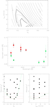 |
Fig. B.1. Oxygen analysis for HD 36512 (O9.7 V) (#1). Upper panel: |

An example for our nitrogen analysis is displayed in Fig. B.2, for HD 12993 (O6.5 V((f)) Nstr) (#8). The innermost contour occurring in the upper panel, at ϵN ~ 8.35 and vmic ~ 16, represents the model with the lowest χ2. The middle panel stresses the good reproduction of the observed lines used in the χ2 -minimization. The lower panel confirms the estimate of the upper plot: the lowest χ2 is found for the model calculated with ϵN = 8.33, and from a broad distribution centered at vmic = 15 km s−1. Since, for this target, the carbon and oxygen analysis suggests vmic = 20 km s−1 as the best-fitting value, we decided to quote this higher vmic as a general value (see discussion in Sect. 4.3).
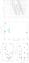 |
Fig. B.2. As Fig. B.1, but for nitrogen in HD12993 (O6.5 V((f)) Nstr) (#8). In this case, all nitrogen lines are well reproduced. |
Finally, Fig. B.3 provides an example for our carbon analysis, in this case for HD 151515 (O7 II(f)) (#18). The upper panel displays a somewhat degenerate solution, with lowest χ2 between 8.3 < ϵC < 8.6, and a large range of possible vmic values. In the middle panel, the restricted number of carbon lines is clearly visible, which are well reproduced. The lower panel allows us to find tighter constraints than the uppermost one. The best-fitting model is given by ϵC ~ 8.43, and the optimum vmic can be limited by ≳15 km s−1, though the other two elements require an even higher limit, ≳20 km s−1.
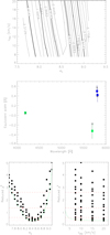 |
Fig. B.3. As Fig. B.1, but for carbon in HD151515 (O7 II(f)) (#18). Middle panel: restricted number of carbon lines available in hotter supergiants. Only a lower limit can be estimated for vmic (see text). |
Appendix C: Line profiles
After identifying the best-fitting model (regarding equivalent widths) via our χ2 -minimization, we compared the corresponding synthetic profiles with the observed ones. Since now the equivalent widths should agree (on average, and except for non-reproducible lines), also the profiles should agree, if rotational and macroturbulent broadening are accounted for. Since we relied on the v sin i values inferred by Holgado et al. (2018), we only checked for vmac, and adapted this value when necessary (see Sect. 5.2), by means of a simple by-eye inspection.
Figures C.1–C.3 provide instructive examples for the agreement or disagreement between synthetic and observed line profiles, for the same stars used in the previous Appendix B, but now for all analyzed elements. For the sake of clarity, the theoretical profiles have different colors, black for carbon, blue for nitrogen, and red for oxygen.
Figure C.1 shows the comparison for basically all of our target lines from HD 36512 (#1). For this star, just a few lines have not been used in our χ2 minimization, namely: C II 3918, 6582; C III 4650, 4651, 5696; N II 4601, 4621; N III 4379, 4641. Moreover, N IV 6380, and the N V lines are not visible in the observed spectrum, and are therefore not included in our analysis.
The carbon and nitrogen lines are generally well reproduced, except for the triplet N III 4634/4640/4641, which, particularly in this temperature range, shows a transition from being refilled into weak emission, and cannot be reproduced by the current FASTWIND version. For details and the origin of this problem, we refer to Rivero González et al. (2011). Also, for all of our oxygen target lines there is a satisfactory agreement, aside from O III 5592 which indicates a higher oxygen abundance, as already obvious from the comparison of equivalent widths (Fig. B.1, middle panel).
For hotter objects as HD 12993 (#8), the analysis becomes more challenging. From Fig. C.2, it is obvious that C II, N II, and O II lines can no longer be used. Rotation adds to these difficulties. In this case, we used the following lines for the χ2 minimization: C III 4186, 4647, 4650, 5696; C IV 5801, 5811; N III 4097, 4379, 4511, 4515, 4518; N IV 4058, 6380; O III 3961, 4081, 5592. Though the C II lines are basically indistinguishable from the continuum, most of the C III and C IV lines are reproduced (except for C III 5696, which is in a transition phase from absorption to emission, and would require a fine-tuning of the wind description to become improved, if at all). The triplet N III 4634/4640/4641 is in emission, but even though we did not use these lines in our minimization, since the equivalent widths are difficult to estimate, they agree reasonably well with our best-fitting model. As pointed out (and discussed) in the main section, for hotter objects the oxygen abundance estimated from O III 5592 (mostly) agrees with the one derived from the other O III lines, as visible in the last panels. For this and similar objects, we have to rely on the calculated oxygen ionization balance, and have no means to check it, except for the fact that all O II lines should be absent in the theoretical spectra.
For HD 151515 (O7 II(f)) (#18), the number of suitable lines is even more restricted than for the hot dwarf described just above. From Fig. C.3, we see that only few lines are detectable, whereas the majority is embedded in the noise. In this case, we could use C III 4186, 5696; C IV 5801, 5811; N III 4097, 4379, 4511, 4515, 4518, 4634, 4640; N IV 4058; O III 5508, 5592. In comparison to the observations, the synthetic C III 4647 profile is too strong, while C III 5696 is too weak. The C IV lines show a slight asymmetry, but even though we have a fair representation. The triplet N III 4634/4640/4641 is clearly in emission, and our theoretical emission lines are too weak (improved wind description required), but all other nitrogen lines are well reproduced. Oxygen displays only few lines, but all of them as calculated from our best-fitting model, and including O III 5592, show a good agreement.
 |
Fig. C.1. HD 36512 (O9.7 V) (#1). Comparison of observed (green) and synthetic line profiles: black – carbon; blue – nitrogen; red – oxygen. The lines N IV 6380, N V 4603, and NV 4619 are not visible (neither in the observations nor in the synthetic spectra), and are not displayed in this figure. |
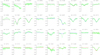 |
Fig. C.2. As Fig. C.1, but for HD 12993 (O6.5 V((f)) Nstr) (#8). N II 3995, 4601, and the N V lines are not visible (neither in the observations nor in the synthetic spectra), and have been skipped in this figure. |
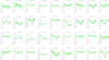 |
Fig. C.3. As Fig. C.1, but for HD 151515 (O7 II(f)) (#18). As in the previous figure, the lines N II 3995, 4601 and N V 4447 are not visible and therefore not displayed. |
References
- Asplund, M., Grevesse, N., Sauval, A. J., & Scott, P. 2009, ARA&A, 47, 481 [NASA ADS] [CrossRef] [Google Scholar]
- Barbá, R. H., Gamen, R., Arias, J. I., et al. 2010, Rev. Mex. Astron. Astrofis., 38, 30 [Google Scholar]
- Barbá, R. H., Gamen, R., Arias, J. I., & Morrell, N. I. 2017, in The Lives and Death-Throes of Massive Stars, eds. J. J. Eldridge, J. C. Bray, L. A. S. McClelland, & L. Xiao, IAU Symp., 329, 89 [NASA ADS] [Google Scholar]
- Behrend, R., & Maeder, A. 2001, A&A, 373, 190 [NASA ADS] [CrossRef] [EDP Sciences] [Google Scholar]
- Bernasconi, P. A., & Maeder, A. 1996, A&A, 307, 829 [NASA ADS] [Google Scholar]
- Bolton, C. T., & Rogers, G. L. 1978, ApJ, 222, 234 [NASA ADS] [CrossRef] [Google Scholar]
- Bouret, J.-C., Hillier, D. J., Lanz, T., & Fullerton, A. W. 2012, A&A, 544, A67 [NASA ADS] [CrossRef] [EDP Sciences] [Google Scholar]
- Bouret, J.-C., Lanz, T., Martins, F., et al. 2013, A&A, 555, A1 [NASA ADS] [CrossRef] [EDP Sciences] [Google Scholar]
- Boyajian, T. S., Beaulieu, T. D., Gies, D. R., et al. 2005, ApJ, 621, 978 [NASA ADS] [CrossRef] [Google Scholar]
- Brott, I., de Mink, S. E., Cantiello, M., et al. 2011, A&A, 530, A115 [NASA ADS] [CrossRef] [EDP Sciences] [Google Scholar]
- Cantiello, M., Langer, N., Brott, I., et al. 2009, A&A, 499, 279 [NASA ADS] [CrossRef] [EDP Sciences] [Google Scholar]
- Carneiro, L. P., Puls, J., Sundqvist, J. O., & Hoffmann, T. L. 2016, A&A, 590, A88 [NASA ADS] [CrossRef] [EDP Sciences] [Google Scholar]
- Carneiro, L. P., Puls, J., & Hoffmann, T. L. 2018, A&A, 615, A4 [NASA ADS] [CrossRef] [EDP Sciences] [Google Scholar]
- Castro, N., Fossati, L., Langer, N., et al. 2014, A&A, 570, L13 [NASA ADS] [CrossRef] [EDP Sciences] [Google Scholar]
- Chiosi, C. 1986, in Luminous Stars and Associations in Galaxies, eds. C. W. H. De Loore, A. J. Willis, & P. Laskarides, IAU Symp., 116, 317 [NASA ADS] [Google Scholar]
- Cohen, D. H., Wollman, E. E., Leutenegger, M. A., et al. 2014, MNRAS, 439, 908 [NASA ADS] [CrossRef] [Google Scholar]
- Crowther, P. A., Hillier, D. J., Evans, C. J., et al. 2002, ApJ, 579, 774 [NASA ADS] [CrossRef] [Google Scholar]
- de Mink, S. E., Langer, N., Izzard, R. G., Sana, H., & de Koter A. 2013, ApJ, 764, 166 [NASA ADS] [CrossRef] [Google Scholar]
- Dufton, P. L., Langer, N., Dunstall, P. R., et al. 2013, A&A, 550, A109 [NASA ADS] [CrossRef] [EDP Sciences] [Google Scholar]
- Ekström, S., Georgy, C., Eggenberger, P., et al. 2012, A&A, 537, A146 [NASA ADS] [CrossRef] [EDP Sciences] [Google Scholar]
- Evans, C., Hunter, I., Smartt, S., et al. 2008, The Messenger, 131, 25 [NASA ADS] [Google Scholar]
- Evans, C. J., Taylor, W. D., Hénault-Brunet, V., et al. 2011, A&A, 530, A108 [NASA ADS] [CrossRef] [EDP Sciences] [Google Scholar]
- Feiveson, A., & Delaney, F. 1968, The Distribution and Properties of a Weighted Sum of Chi Squares, NASA technical note (National Aeronautics and Space Administration) [Google Scholar]
- Feldmeier, A., Puls, J., & Pauldrach, A. W. A. 1997, A&A, 322, 878 [NASA ADS] [Google Scholar]
- Garmany, C. D., Conti, P. S., & Chiosi, C. 1982, ApJ, 263, 777 [NASA ADS] [CrossRef] [Google Scholar]
- Grin, N. J., Ramírez-Agudelo, O. H., de Koter, A., et al. 2017, A&A, 600, A82 [NASA ADS] [CrossRef] [EDP Sciences] [Google Scholar]
- Haemmerlé, L., Eggenberger, P., Meynet, G., Maeder, A., & Charbonnel, C. 2016, A&A, 585, A65 [NASA ADS] [CrossRef] [EDP Sciences] [Google Scholar]
- Hamann, W.-R., & Oskinova, L. 2012, COSPAR Meeting, 39th COSPAR Scientific Assembly, 39, 716 [NASA ADS] [Google Scholar]
- Heger, A., Langer, N., & Woosley, S. E. 2000, ApJ, 528, 368 [NASA ADS] [CrossRef] [Google Scholar]
- Herrero, A., Kudritzki, R. P., Vilchez, J. M., et al. 1992, A&A, 261, 209 [NASA ADS] [Google Scholar]
- Herrero, A., Simon-Diaz, S., Najarro, F., & Ribas, I. 2007, in Massive Stars in Interactive Binaries, eds. N. St.-Louis & A. F. J. Moffat, ASP Conf. Ser., 367, 67 [NASA ADS] [Google Scholar]
- Hillier, D. J., & Miller, D. L. 1998, ApJ, 496, 407 [NASA ADS] [CrossRef] [Google Scholar]
- Hillier, D. J., Kudritzki, R. P., Pauldrach, A. W., et al. 1993, A&A, 276, 117 [NASA ADS] [Google Scholar]
- Holgado, G., Simón-Díaz, S., Barbá, R. H., et al. 2018, A&A, 613, A65 [NASA ADS] [CrossRef] [EDP Sciences] [Google Scholar]
- Howarth, I. D., Siebert, K. W., Hussain, G. A. J., & Prinja, R. K. 1997, MNRAS, 284, 265 [NASA ADS] [CrossRef] [Google Scholar]
- Hunter, I., Dufton, P. L., Smartt, S. J., et al. 2007, A&A, 466, 277 [NASA ADS] [CrossRef] [EDP Sciences] [Google Scholar]
- Hunter, I., Brott, I., Lennon, D. J., et al. 2008, ApJ, 676, L29 [NASA ADS] [CrossRef] [Google Scholar]
- Kaufer, A., Wolf, B., Andersen, J., & Pasquini, L. 1997, The Messenger, 89, 1 [NASA ADS] [Google Scholar]
- Kelleher, D. E., Mohr, P. J., Martin, W. C., et al. 1999, SPIE Conf. Ser., 3818, 170 [NASA ADS] [CrossRef] [Google Scholar]
- Keszthelyi, Z., Puls, J., & Wade, G. A. 2017, A&A, 598, A4 [NASA ADS] [CrossRef] [EDP Sciences] [Google Scholar]
- Köhler, K., Langer, N., de Koter, A., et al. 2015, A&A, 573, A71 [NASA ADS] [CrossRef] [EDP Sciences] [Google Scholar]
- Kudritzki, R.-P., & Puls, J. 2000, ARA&A, 38, 613 [NASA ADS] [CrossRef] [Google Scholar]
- Kupka, F., Piskunov, N., Ryabchikova, T. A., Stempels, H. C., & Weiss, W. W. 1999, A&AS, 138, 119 [NASA ADS] [CrossRef] [EDP Sciences] [MathSciNet] [PubMed] [Google Scholar]
- Kupka, F. G., Ryabchikova, T. A., Piskunov, N. E., Stempels, H. C., & Weiss, W. W. 2000, Balt. Astron., 9, 590 [NASA ADS] [Google Scholar]
- Langer, N. 2012, ARA&A, 50, 107 [NASA ADS] [CrossRef] [Google Scholar]
- Langer, N., & Kudritzki, R. P. 2014, A&A, 564, A52 [NASA ADS] [CrossRef] [EDP Sciences] [Google Scholar]
- Langer, N., Heger, A., & Fliegner, J. 1997, IAU Symp., 189, 343 [NASA ADS] [Google Scholar]
- Langer, N., Cantiello, M., Yoon, S.-C., et al. 2008, in Massive Stars as Cosmic Engines, eds. F. Bresolin, P. A. Crowther, & J. Puls, IAU Symp., 250, 167 [Google Scholar]
- Lefever, K. 2007, Ph.D. Thesis, Catholic University Leuven, Belgium [Google Scholar]
- Maeder, A. 1976, A&A, 47, 389 [NASA ADS] [Google Scholar]
- Maeder, A. 2009, Physics, Formation and Evolution of Rotating Stars (Berlin: Springer) [Google Scholar]
- Maeder, A., Przybilla, N., Nieva, M.-F., et al. 2014, A&A, 565, A39 [NASA ADS] [CrossRef] [EDP Sciences] [Google Scholar]
- Maíz Apellániz, J., Alfaro, E. J., Arias, J. I., et al. 2015, in Highlights of Spanish Astrophysics VIII, eds. A. J. Cenarro, F. Figueras, C. Hernández-Monteagudo, et al. (Dordrecht: The Netherlands), 603 [Google Scholar]
- Markova, N., & Puls, J. 2008, A&A, 478, 823 [NASA ADS] [CrossRef] [EDP Sciences] [Google Scholar]
- Markova, N., Puls, J., & Langer, N. 2018, A&A, 613, A12 [NASA ADS] [CrossRef] [EDP Sciences] [Google Scholar]
- Martins, F., & Hillier, D. J. 2012, A&A, 545, A95 [NASA ADS] [CrossRef] [EDP Sciences] [Google Scholar]
- Martins, F., Schaerer, D., & Hillier, D. J. 2005, A&A, 436, 1049 [NASA ADS] [CrossRef] [EDP Sciences] [Google Scholar]
- Martins, F., Simón-Díaz, S., Palacios, A., et al. 2015a, A&A, 578, A109 [NASA ADS] [CrossRef] [EDP Sciences] [Google Scholar]
- Martins, F., Hervé, A., Bouret, J.-C., et al. 2015b, A&A, 575, A34 [NASA ADS] [CrossRef] [EDP Sciences] [Google Scholar]
- Martins, F., Foschino, S., Bouret, J.-C., Barbá, R., & Howarth, I. 2016, A&A, 588, A64 [NASA ADS] [CrossRef] [EDP Sciences] [Google Scholar]
- Martins, F., Simón-Díaz, S., Barbá, R. H., Gamen, R. C., & Ekström, S. 2017, A&A, 599, A30 [NASA ADS] [CrossRef] [EDP Sciences] [Google Scholar]
- Meynet, G., & Maeder, A. 2000, A&A, 361, 101 [NASA ADS] [Google Scholar]
- Mihalas, D., & Hummer, D. G. 1973, ApJ, 179, 827 [NASA ADS] [CrossRef] [Google Scholar]
- Mokiem, M. R., de Koter, A., Puls, J., et al. 2005, A&A, 441, 711 [NASA ADS] [CrossRef] [EDP Sciences] [Google Scholar]
- Najarro, F., Hanson, M. M., & Puls, J. 2011, A&A, 535, A32 [NASA ADS] [CrossRef] [EDP Sciences] [Google Scholar]
- Nussbaumer, H., & Storey, P. J. 1983, A&A, 126, 75 [NASA ADS] [Google Scholar]
- Oskinova, L. M., Hamann, W.-R., & Feldmeier, A. 2007, A&A, 476, 1331 [NASA ADS] [CrossRef] [EDP Sciences] [Google Scholar]
- Owocki, S. P. 2008, in Clumping in Hot-Star Winds, eds. W.-R. Hamann, L. M. Oskinova, & A. Feldmeier (Potsdam: Universitätsverlag Potsdam), 121 [Google Scholar]
- Owocki, S. P., Sundqvist, J. O., Cohen, D. H., & Gayley, K. G. 2013, MNRAS, 429, 3379 [NASA ADS] [CrossRef] [Google Scholar]
- Pauldrach, A. W. A., Kudritzki, R. P., Puls, J., Butler, K., & Hunsinger, J. 1994, A&A, 283, 525 [Google Scholar]
- Pauldrach, A. W. A., Hoffmann, T. L., & Lennon, M. 2001, A&A, 375, 161 [NASA ADS] [CrossRef] [EDP Sciences] [Google Scholar]
- Paxton, B., Cantiello, M., Arras, P., et al. 2013, ApJS, 208, 4 [NASA ADS] [CrossRef] [Google Scholar]
- Piskunov, N. E., Kupka, F., Ryabchikova, T. A., Weiss, W. W., & Jeffery, C. S. 1995, A&AS, 112, 525 [NASA ADS] [Google Scholar]
- Przybilla, N., Nieva, M., & Butler, K. 2008, ApJ, 688, L103 [NASA ADS] [CrossRef] [Google Scholar]
- Przybilla, N., Firnstein, M., Nieva, M. F., Meynet, G., & Maeder, A. 2010, A&A, 517, A38 [NASA ADS] [CrossRef] [EDP Sciences] [Google Scholar]
- Puls, J., Urbaneja, M. A., Venero, R., et al. 2005, A&A, 435, 669 [NASA ADS] [CrossRef] [EDP Sciences] [Google Scholar]
- Ramírez-Agudelo, O. H., Simón-Díaz, S., Sana, H., et al. 2013, A&A, 560, A29 [NASA ADS] [CrossRef] [EDP Sciences] [Google Scholar]
- Raskin, G., Van Winckel, H., & Davignon, G. 2004, in Ground-Based Instrumentation for Astronomy, eds. A. F. M. Moorwood & M. Iye, Proc. SPIE, 5492, 322 [NASA ADS] [CrossRef] [Google Scholar]
- Repolust, T., Puls, J., & Herrero, A. 2004, A&A, 415, 349 [NASA ADS] [CrossRef] [EDP Sciences] [Google Scholar]
- Rivero González, J. G., Puls, J., & Najarro, F. 2011, A&A, 536, A58 [NASA ADS] [CrossRef] [EDP Sciences] [Google Scholar]
- Rivero González, J. G., Puls, J., Najarro, F., & Brott, I. 2012a, A&A, 537, A79 [NASA ADS] [CrossRef] [EDP Sciences] [Google Scholar]
- Rivero González, J. G., Puls, J., Najarro, F., & Massey, P. 2012b, A&A, 543, A95 [NASA ADS] [CrossRef] [EDP Sciences] [Google Scholar]
- Ryabchikova, T. A., Piskunov, N. E., Kupka, F., & Weiss, W. W. 1997, Bal. Astron., 6, 244 [Google Scholar]
- Ryabchikova, T., Piskunov, N., Kurucz, R. L., et al. 2015, Phys. Scr, 90, 054005 [NASA ADS] [CrossRef] [Google Scholar]
- Sabín-Sanjulián, C., Simón-Díaz, S., Herrero, A., et al. 2017, A&A, 601, A79 [NASA ADS] [CrossRef] [EDP Sciences] [Google Scholar]
- Seaton, M. J. 1958, MNRAS, 118, 504 [NASA ADS] [CrossRef] [Google Scholar]
- Simón-Díaz, S. 2010, A&A, 510, A22 [NASA ADS] [CrossRef] [EDP Sciences] [Google Scholar]
- Simón-Díaz, S., & Herrero, A. 2007, A&A, 468, 1063 [NASA ADS] [CrossRef] [EDP Sciences] [Google Scholar]
- Simón-Díaz, S., & Herrero, A. 2014, A&A, 562, A135 [NASA ADS] [CrossRef] [EDP Sciences] [Google Scholar]
- Simón-Díaz, S., Castro, N., Herrero, A., et al. 2011, J. Phys. Conf. Ser., 328, 012021 [NASA ADS] [CrossRef] [Google Scholar]
- Simón-Díaz, S., Herrero, A., Sabín-Sanjulián, C., et al. 2014, A&A, 570, L6 [NASA ADS] [CrossRef] [EDP Sciences] [Google Scholar]
- Simón-Díaz, S., Negueruela, I., Maíz Apellániz, J., et al. 2015, in Highlights of Spanish Astrophysics VIII, eds. A. J. Cenarro, F. Figueras, C. Hernández-Monteagudo, et al. (Dordrecht: The Netherlands), 576 [Google Scholar]
- Smith, K. C., & Howarth, I. D. 1998, MNRAS, 299, 1146 [NASA ADS] [CrossRef] [Google Scholar]
- Sota, A., Maíz Apellániz, J., Walborn, N. R., et al. 2011, ApJS, 193, 24 [NASA ADS] [CrossRef] [Google Scholar]
- Sundqvist, J. O., & Puls, J. 2018, A&A, 619, A59 [NASA ADS] [CrossRef] [EDP Sciences] [Google Scholar]
- Sundqvist, J. O., Puls, J., & Feldmeier, A. 2010, A&A, 510, A11 [NASA ADS] [CrossRef] [EDP Sciences] [Google Scholar]
- Sundqvist, J. O., Puls, J., & Owocki, S. P. 2014, A&A, 568, A59 [NASA ADS] [CrossRef] [EDP Sciences] [Google Scholar]
- Šurlan, B., Hamann, W.-R., Aret, A., et al. 2013, A&A, 559, A130 [NASA ADS] [CrossRef] [EDP Sciences] [Google Scholar]
- Telting, J. H., Avila, G., Buchhave, L., et al. 2014, Astron. Nachr., 335, 41 [NASA ADS] [CrossRef] [Google Scholar]
- Urbaneja, M. 2004, Ph.D. Thesis, Universidad de la Laguna, La Laguna, Spain [Google Scholar]
- Villamariz, M. R., Herrero, A., Becker, S. R., & Butler, K. 2002, A&A, 388, 940 [NASA ADS] [CrossRef] [EDP Sciences] [Google Scholar]
- Vink, J. S., Brott, I., Gräfener, G., et al. 2010, A&A, 512, L7 [NASA ADS] [CrossRef] [EDP Sciences] [Google Scholar]
We are aware of the additional problem of blends, but (a) for our slowly rotating objects they are of minor concern, and (b) in many cases we could estimate their EW by fitting the uncontaminated part as described in Sect. 4.1.
By means of precalculated grids of synthetic spectra and the IACOB-GBAT tool (Simón-Díaz et al. 2011).
In contrast to the present approach, Carneiro et al. (2018) used a by eye fitting method.
https://www.nist.gov/pml/atomic-spectra-database, described by Kelleher et al. (1999).
http://vald.astro.uu.se/~vald/php/vald.php, described by Piskunov et al. (1995), Ryabchikova et al. (1997, 2015), and Kupka et al. (1999, 2000).
For a detailed investigation of the sensitivity of theoretical EW values as a function of abundance for nitrogen lines, we refer to Grin et al. (2017), who also discuss certain limitations and the impact of varying vmic.
That is, if the value provided by Holgado et al. (2018) resulted in problematic line shapes.
Assuming the so called dilution factor – in other words, the fraction of the mass with initial composition divided by the total mass which is mixed – as close to unity, the initial values of the ratios can be used instead of the abundances after CN equilibrium (for further details, see Maeder et al. 2014).
To enable a comparison with objects from this cluster within the VLT-FLAMES survey on massive stars, the latter summarized by Evans et al. (2008).
gtrue = gspec + gcent, with 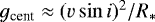 (Repolust et al. 2004). In our sample, the maximum difference between log gtrue and log gspec is ≲0.02 dex when the stellar radius has been estimated from typical calibrations (e.g., Martins et al. 2005).
Recall that our sample is a subsample from the objects studied by Holgado et al. (2018), thus our finding is not surprising.
For a comparison between results from the conventional and the spectroscopic HR diagram, see again Markova et al. (2018).
Defined by Sota et al. (2011, their Table 3) as a moderate case of enhanced N absorption, with C and O deficient.
These similar ϵC and different ϵN values that are finally reached lead to the slightly diverging curves found in Fig. 5.
All Tables
Stellar, wind, and line-broadening parameters for the finally analyzed 18 sample stars.
Diagnostic carbon, nitrogen, and oxygen lines in the optical spectrum, used to derive corresponding abundances of O-type stars.
Carbon, nitrogen and oxygen abundances obtained from our analysis, and the best-fitting vmic for the CNO lines.
Initial values of CNO abundances adopted in the evolutionary grids referred to in this work, and corresponding solar values from Asplund et al. (2009).
All Figures
|
Fig. 1. Relation between nitrogen-to-carbon and nitrogen-to-oxygen ratios. Left panel: our results with (approximate) errors when including the uncertainties in Teff and log g. Right panel: only those uncertainties that arise from our method when relying on the Teff and log g values provided by Holgado et al. (2018; see Sect. 5.1). “Hot” and “cold” dwarfs are denoted by blue and red squares, and hot and cold supergiants/bright giants by cyan and magenta asterisks. For our division between hot and cold objects, and the correspondence between number and object, see Table 3. The solid lines represent the theoretical limits for the early phases of the CNO cycle (less massive stars), and for the conversion of O to N after afast establishment of CN equilibrium (most massive stars). Both curves adopt the initial abundances from the Geneva models (Ekström et al. 2012, see Sect. 6.1 and Table 4). |
| In the text | |
|
Fig. 2. Differences between the logarithmic chemical abundances obtained in the present work and those from Martins et al. (2015b, 2017; colored symbols as in Fig. 1) and Markova et al. (2018; nitrogen only, black circles). Errors of own data include typical uncertainties in stellar parameters. |
| In the text | |
|
Fig. 3. Left panel: Kiel diagram (log g vs. Teff) for our sample stars. Overplotted are the rotating Geneva (Ekström et al. 2012; black) and Bonn (Brott et al. 2011; red) tracks for the mass range 20–60 M⊙, with initial rotation velocities of 40% of their critical speed. Right panel: corresponding spectroscopy HR diagram (sHRD, see text), with both ordinate-axes proportional to L∕M. The Eddington Γe has been calculated with solar Helium content, assumed to be completely ionized. Symbols in both panels as in Fig. 1. |
| In the text | |
|
Fig. 4. Modified sHRD, with abscissa log g (instead of Teff), providing a clearer separation between the tracks. Two distinct gravity regimes populated by our sample stars become obvious (see text). |
| In the text | |
|
Fig. 5. Relation ϵC vs. ϵN in the light of evolutionary tracks. The black and red lines display the corresponding Geneva and Bonn tracks with |
| In the text | |
|
Fig. 6. Evolution of C/N/O abundances for different masses (from left to right panels: 60, 40, ~30, 25, and 20 M⊙) as a functionof Teff, as predicted by the rotating Geneva (black lines, left panels) and Bonn tracks (red lines, right panels). The dotted line represents the solar abundance. The dashed and the dash-dotted lines display the initial abundances used in the Geneva andin the Bonn calculations, respectively. Our results (symbols as in Fig. 1) are shown with errors accounting for typical uncertainties in stellar parameters. For initial evolutionary masses of sample stars, see Table 5. |
| In the text | |
|
Fig. 7. Nitrogen-to-carbon ratio vs. v sin i for our sample stars. The dotted line represents the solar value. |
| In the text | |
|
Fig. A.1. Examples for equivalent width measurements via Gaussian fits (blue) and direct integration (with respect to the interval indicated in red): C III 5696, N III 4514, and O III 3961, in the spectrum of HD 46966 (#6). |
| In the text | |
|
Fig. B.1. Oxygen analysis for HD 36512 (O9.7 V) (#1). Upper panel: |
| In the text | |
|
Fig. B.2. As Fig. B.1, but for nitrogen in HD12993 (O6.5 V((f)) Nstr) (#8). In this case, all nitrogen lines are well reproduced. |
| In the text | |
|
Fig. B.3. As Fig. B.1, but for carbon in HD151515 (O7 II(f)) (#18). Middle panel: restricted number of carbon lines available in hotter supergiants. Only a lower limit can be estimated for vmic (see text). |
| In the text | |
|
Fig. C.1. HD 36512 (O9.7 V) (#1). Comparison of observed (green) and synthetic line profiles: black – carbon; blue – nitrogen; red – oxygen. The lines N IV 6380, N V 4603, and NV 4619 are not visible (neither in the observations nor in the synthetic spectra), and are not displayed in this figure. |
| In the text | |
|
Fig. C.2. As Fig. C.1, but for HD 12993 (O6.5 V((f)) Nstr) (#8). N II 3995, 4601, and the N V lines are not visible (neither in the observations nor in the synthetic spectra), and have been skipped in this figure. |
| In the text | |
|
Fig. C.3. As Fig. C.1, but for HD 151515 (O7 II(f)) (#18). As in the previous figure, the lines N II 3995, 4601 and N V 4447 are not visible and therefore not displayed. |
| In the text | |
Current usage metrics show cumulative count of Article Views (full-text article views including HTML views, PDF and ePub downloads, according to the available data) and Abstracts Views on Vision4Press platform.
Data correspond to usage on the plateform after 2015. The current usage metrics is available 48-96 hours after online publication and is updated daily on week days.
Initial download of the metrics may take a while.