| Issue |
A&A
Volume 623, March 2019
|
|
|---|---|---|
| Article Number | A76 | |
| Number of page(s) | 14 | |
| Section | Cosmology (including clusters of galaxies) | |
| DOI | https://doi.org/10.1051/0004-6361/201833732 | |
| Published online | 07 March 2019 | |
Impact of photometric redshifts on the galaxy power spectrum and BAO scale in the LSST survey
1
LAL, Univ. Paris-Sud, CNRS/IN2P3, Université Paris-Saclay, Orsay, France
2
Univ. Grenoble Alpes, CNRS, Grenoble INP, LPSC-IN2P3, 38000 Grenoble, France
e-mail: This email address is being protected from spambots. You need JavaScript enabled to view it.
3
DSM/Irfu/SPP, CEA-Saclay, 91191 Gif-sur-Yvette Cedex, France
Received:
28
June
2018
Accepted:
28
January
2019
Abstract
Context. The Large Synoptic Survey Telescope (LSST) survey will image billions of galaxies every few nights for ten years, and as such, should be a major contributor to precision cosmology in the 2020s. High precision photometric data will be available in six bands, from near-infrared to near-ultraviolet. The computation of precise, unbiased, photometric redshifts up to at least z = 2 is one of the main LSST challenges and its performance will have major impact on all extragalactic LSST sciences.
Aims. We evaluate the efficiency of our photometric redshift reconstruction on mock galaxy catalogues up to z = 2.45 and estimate the impact of realistic photometric redshift (photo-z) reconstruction on the large-scale structures (LSS) power spectrum and the baryonic acoustic oscillation (BAO) scale determination for a LSST-like photometric survey. We study the effectiveness of the BAO scale as a cosmological probe in the LSST survey.
Methods. We have performed a detailed modelling of the photo-z distribution as a function of galaxy type, redshift and absolute magnitude using our photo-z reconstruction code with a quality selection cut based on a boosted decision tree (BDT). We have simulated a catalogue of galaxies in the redshift range [0.2−2.45] using the Planck 2015 ΛCDM cosmological parameters over 10 000 square-degrees, in the six bands, assuming LSST photometric precision for a ten-year survey. The mock galaxy catalogues were produced with several redshift error models. The LSS power spectrum was then computed in several redshift ranges and for each error model. Finally we extracted the BAO scale and its uncertainty using only the linear part of the LSS spectrum.
Results. We have computed the fractional error on the recovered power spectrum which is dominated by the shot noise at high redshift (z ≳ 1), for scales k ≳ 0.1, due to the photo-z damping. The BAO scale can be recovered with a percent or better accuracy level from z = 0.5 to z = 1.5 using realistic photo-z reconstruction.
Conclusions. Reaching the LSST requirements for photo-z reconstruction is crucial to exploit the LSST potential in cosmology, in particular to measure the LSS power spectrum and its evolution with redshift. Although the BAO scale is not the most powerful cosmological probe in LSST, it can be used to check the consistency of the LSS measurement. Moreover we show that the impact of photo-z smearing on the recovered isotropic BAO scale in LSST should stay limited up to z ≈ 1.5, so as long as the galaxy number density balances the photo-z smoothing.
Key words: large-scale structure of Universe / galaxies: distances and redshifts
© R. Ansari et al. 2019
 Open Access article, published by EDP Sciences, under the terms of the Creative Commons Attribution License (http://creativecommons.org/licenses/by/4.0), which permits unrestricted use, distribution, and reproduction in any medium, provided the original work is properly cited.
1. Introduction
The six-band (ugrizy) Large Synoptic Survey Telescope (LSST) survey, described in LSST Science Collaboration et al. (2009), will yield a sample of about ten billion galaxies over a huge volume. It will be the largest photometric galaxy sample of the next decade to study the large-scale structures (LSS) of the Universe. It aims to characterise the distribution and evolution of matter on extragalactic scales through observations of baryonic matter at a broad range of wavelengths. The LSS encodes crucial information about the content of the Universe, the origin of the fluctuations and the cosmic expansion background in which the structures evolve. Of particular interest is the imprint on galaxy clustering of baryon acoustic oscillations (BAO), which reflects the acoustic waves at recombination, related to the sound horizon at that epoch. The BAO scale is sufficiently small that it is possible to measure it precisely with a large volume survey; yet, this scale is large enough that it is not significantly altered by non-linear evolution. The BAO features can be used as a standard to measure distances and constrain the dark energy equation of state, especially when used in combination with weak lensing.
Every few nights the LSST will observe half of the whole sky up to a magnitude of 24. After ten years of survey, the depth of the stacked images should reach magnitude 27 in the i-band and LSST should provide a catalogue of a few billions of galaxies with a photometry good enough to be useable for cosmology. Indeed, doing cosmology implies accurate knowledge of the galaxy positions. While the angular coordinates will be exquisitely measured thanks to the LSST optics and camera design, it will be much more challenging to reconstruct the third coordinate, the redshift.
Results using spectroscopic data of the BOSS survey Dawson et al. (2013), part of the Sloan Digital Sky Survey III, allow precise measurement of the BAO scale and lead to accurate cosmological parameters, for instance Anderson et al. (2012), Aubourg et al. (2015) or more recently Salazar-Albornoz et al. (2017), Alam et al. (2017). Although BAO constraints with LSST might be not fully competitive with the future spectroscopic survey DESI Levi et al. (2013) or later Euclid Laureijs et al. (2011), performing BAO analysis is crucial to cross-correlate the results with those of other LSST probes. The reader can refer to Zhan & Tyson (2018) and references therein for a recent review of the cosmology reach of LSST, including the BAO probe. The sensitivity of each probe to systematic errors and to dark energy parameters is different, so it is mandatory to check the consistency of all results, and powerful to combine them Alonso et al. (2017). The study of BAO in LSST can, in return, be a way to test our photo-z reconstruction and tune the quality cuts to deal with the total number of galaxies versus the number of outliers. The current DES survey Drinkwater et al. (2010), with only five filters, has already faced similar challenges Crocce et al. (2019), obtaining a 4% distance measurement of the standard ruler Abbott et al. (2019).
The goal of this paper is to test the impact of the use of photo-z to reconstruct the LSS power spectrum, considering several options on the required quality up to z = 2.2. Compared to some previous work on BAO with photometric redshifts in LSST Zhan et al. (2009), Abrahamse et al. (2011) where simpler LSST observation and photo-z error model were used, we have carried out a complete analysis using realistic mock galaxy catalogues with galaxies. The cosmological impact is illustrated by comparing the BAO scales measured using spectroscopic redshifts (hereafter spectro-z) or photo-z of galaxies from a mock catalogue; our BAO analysis is similar to the method described in Blake et al. (2011). The BAO scale extraction is simply based on the wiggle method described in Beutler et al. (2016a).
The paper is organised as follows. We first present the LSST survey and the goal of the paper. Section 2 is dedicated to an overview of the mock catalogue of galaxies and Sect. 3 presents the photometric redshift reconstruction characteristics and performances. Section 4 presents method and results regarding the matter power spectra and the BAO scale. We have developed a Monte Carlo simulation to easily link precision on the recovered BAO scale and photo-z performances presented in Sect. 5. Finally, we summarise our results in Sect. 6.
2. LSST mock galaxy catalogue simulation and analysis procedure overview
A complete end to end simulation and analysis pipeline has been developed to measure the performance of a LSST-like photometric survey for recovering the LSS power spectrum. Starting from a set of cosmological parameters and going through mock galaxy catalogues with realistic photo-z, the pipeline is used to extract the BAO scale at several redshifts. The main blocks of this pipeline are depicted in Fig. 1.
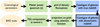 |
Fig. 1. Graphic representation of the main steps of the simulation chain, from cosmological parameters up to the BAO scale measurement. |
We started from the matter power spectrum P(k) computed at a given reference redshift z0, from which a huge grid of density fluctuations δρ/ρ is calculated, through random generation of Fourier coefficients and Fourier transform (FFT). The grid of density field was then converted into a catalogue of galaxies using galaxy luminosity functions (LFs). We used a set of LFs corresponding to different galaxy classes mapped into spectral types. It should be stressed that, in this procedure, we assumed that the local galaxy absolute luminosity is directly proportional to the local matter density (1 + δρ/ρ).
The key ingredient for the study presented here is the error model for assigning “observed” redshifts to the galaxies. We compared several cases, including a realistic photo-z reconstruction through the FastPz method discussed below.
The mock galaxy catalogue was then analysed: after computation of the redshift dependent selection function, the galaxy angular positions and redshifts are converted into 3D positions using a fiducial cosmology. Galaxies are projected into 3D-grids positioned at several redshifts. The observed power spectrum Pz(k) for each redshift range is computed through a Fourier transform, averaging over all Fourier modes within a k-bin. Finally, the BAO scale and its uncertainty were extracted from the ratio of Pz(k) to a wiggle-less power spectrum through a dedicated fit procedure described in Sect. 4.3 and compared to the expected value from the input cosmological parameters.
This pipeline produces a catalogue directly, so we could ignore all systematics introduced by the catalogue extraction from the images, even if effects such as blending Jones & Heavens (2019) or dithering Awan et al. (2016) affect photometric and spectroscopic surveys in different ways. The simplistic way that galaxy catalogues are produced does not allow us to derive the precision of the effective reconstruction of the matter power spectrum by LSST. However, this methodology and the following analyses are well suited to evaluate the impact of realistic photo-z redshifts, compared to spectro-z redshifts, on the matter power spectrum, and more specifically on the reconstruction of the BAO scale.
2.1. Computation of the density field grid
Our aim is to simulate the density field on a large portion of the sky in order to get a simplified view of half of the sky that will be monitored by LSST. We define a volume, hereafter named BigCube, which has a comoving depth of 5600 Mpc along the Oz axis and a transverse comoving section of 10 000 × 10 000 Mpc2. The grid centre is set at 3200 Mpc from the observer. This BigCube is divided into cells of 8 × 8 × 8 Mpc3, a small enough cell size compared to the BAO scale (∼150 Mpc). Some non-linearities may affect the galaxy distribution around or below the cell scale but, for our purpose, we do not need to take into account such additional complexities.
The matter power spectrum is initially computed for the redshift of the BigCube centre with the cosmological parameters of the fiducial model. We used the set of parameters defined in Planck Collaboration XIII (2016) in the conservative case, based on the TT power spectrum with lensing reconstruction, polarisation only at low multi-poles and external data (Col. 3, Table 4): the Hubble constant is then H0 = 67.90 km s−1 Mpc−1, the cold dark matter reduced density is ΩCDM = 0.2582, the baryonic matter reduced density is ΩB = 0.0483 and the (linear) power spectrum is described by a power-law with an amplitude σ8 = 0.8154 at a scale of 8 h−1 Mpc and a spectral index ns = 0.9681. The hypothesis in the ΛCDM model is that the neutrino mass is minimal and the geometry is flat.
Density fluctuations are generated from the power spectrum P(k) using the standard formalism, described for example in Eisenstein & Hu (1998). Fourier components F(k) for the matter density fluctuation field were randomly generated following the power spectrum ⟨|F(k)|2⟩=P(k = |k|). The matter density fluctuation field δρ/ρ was then computed through an FFT on the array of generated Fourier components. We next applied the growth factor to each cell in the cube, according to its redshift. This method is less accurate than the one implemented in CLASS Lesgourgues (2011) but the resulting spectra differ only marginally. This simplified method is sufficient, as our aim is to quantify the loss of information induced by the photo-z reconstruction on the matter power spectrum and we do not try to quantify uncertainties on cosmological parameters.
The density field grid is then clipped, setting cells with δρ/ρ < −1 to −1 to avoid cells with negative matter density. This clipping has no effect on the results presented in this paper, as we use the power spectrum of the clipped grid as the reference power spectrum. We have also checked that the distortions of the power spectrum due to clipping, ranging from a factor 0.5−0.6 to 0.8 depending on the k-scale, do not significantly affect its overall shape and BAO features.
2.2. Simulation of the catalogue
The density fluctuations were then converted into galaxy number fluctuations, assuming proportionality of light to matter density (1 + δρ/ρ). The key ingredient for this step is the use of observed galaxy LF to populate each grid cell with a number of galaxies with absolute magnitudes and galaxy classes or spectral types following the LFs. Details of the procedure are provided in Gorecki et al. (2014), the main difference from our method being that we have used LF parameters derived by Zucca et al. (2009) for the study presented here, instead of the one derived by Dahlen et al. (2005) used in our previous work. Both sets of LFs provide the distribution of galaxies divided in broad types, in several redshift ranges. We have used the Schechter parameters from Zucca et al. (2009) with fixed power law index (α). LF parameters are given for galaxies divided in three broad types, labelled early, late or starburst, corresponding roughly to elliptical, spiral and irregular morphological types. These three broad categories were then mapped into a library of spectral types.
The main steps for converting the density fluctuation grid to a list of galaxies are summarised below:
-
The total number of galaxies N within our survey volume was computed by integrating the LFs with a faint absolute magnitude limit well above the LSST detection threshold at all redshifts. This number N was then used to compute the average number of galaxies per BigCube cell.
-
For each cell, the average number of galaxies in the cell n̄(x) was computed according to the local matter density 1 + δρ/ρ. The number of galaxies in the cell was then drawn with a Poisson distribution with mean n̄(x. Galaxy positions were uniformly generated within each cell, then their angular positions and true redshifts are computed from their positions in the grid. An absolute magnitude and a type were assigned to each galaxy according to the multi-type, redshift dependent LFs. We have chosen to use the Zucca et al. (2009) parametrisation which, once extrapolated to high redshifts, provides a reasonable evolution of the number of galaxies. Only galaxies within a cone with half-opening angle of 60° (defining a solid angle of π, so covering ≈10 000 deg2) are kept. The catalogue in our simulation properly covers the redshifts from 0.2 to 2.45.
-
We used a library of 51 interpolated SEDs from six main SEDs, composed of four SEDs of Coleman et al. (1980): Elliptical, Sbc, Scd or Im, and the two SEDs of Kinney et al. (1996): SB3 and SB2. Galaxies from each LF class are then distributed over a subset of these 51 interpolated SEDs. We then computed the apparent magnitudes in each of the six LSST bands (ugrizy) for each galaxy present in the simulation volume, taking into account the nominal LSST ten-year photometric errors for each band. The photometric errors will depend on the distribution of visits per filter and on the ability to manage the atmospheric properties during observations, as shown in Graham et al. (2018). We note that these errors have been estimated for point-like sources and are applied to extended sources. Only galaxies with mi < 25.3, satisfying the so-called LSST golden selection cut, are kept for the subsequent analysis, allowing a reliable estimate of the photo-z.
As shown and discussed in this paper, the effective density of galaxies observable in LSST as a function of redshift is a crucial ingredient to compute its expected performance for measuring the LSS power spectrum and the BAO scale. Many values of the Schechter parameters describing the LFs can be found in the literature: Ramos et al. (2011), Dahlen et al. (2005), and Zucca et al. (2009) for instance. As expected, LF parameters derived from observations have some uncertainties and one finds significant differences when galaxy densities in the LSST survey are computed from different sets of LFs.
In the left panel of Fig. 2, we show the expected galaxy surface density number as a function of the i-band magnitude limit. We have compared the numbers obtained from the extrapolation used in the LSST Science Collaboration et al. (2009) and numbers derived from Dahlen et al. (2005) and Zucca et al. (2009) LF parameters. These curves are obtained by integrating the LF Schechter functions for each redshift, with the faint end absolute magnitude limit computed from the i-band magnitude limit, taking into account the K-correction and the luminosity distance. The observable galaxy density is then integrated as a function of redshift, over the cosmological volume element. As already pointed out by Chang et al. (2013), for instance, the expected galaxy density used in LSST Science Collaboration et al. (2009) is rather optimistic. Indeed, for the LSST golden selection cut, the science book extrapolation yields ∼55 gal arcmin−2, compared to ∼36 gal arcmin−2 for Dahlen et al. (2005) and ∼41 gal arcmin−2 for Zucca et al. (2009). The initial LSST value of 55 gal arcmin−2 seems to come from a too rough first guess. To explain the discrepancy between the two other sets of LFs, we compare their expected number of galaxies per Mpc3 as a function of redshift for the LSST golden selection cut in the right panel of Fig. 2. The Zucca et al. (2009) LFs lead to a higher galaxy number density at all redshifts above z ≈ 0.6. So, once integrated up to z ≥ 0.8, the surface galaxy number density is higher with this set of Schechter parameters. Moreover the Zucca et al. (2009) LFs provide smoother, and so more realistic, galaxy density evolution along cosmic time.
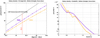 |
Fig. 2. Left panel: expected galaxy surface density as a function of the i-band magnitude limit: comparison of LSST Science Collaboration et al. (2009) extrapolation, numbers derived from the Dahlen et al. (2005) and Zucca et al. (2009) LFs parameters. Right panel: number of galaxies per Mpc3 as a function of redshift, for the LSST golden selection cut from Dahlen et al. (2005) and Zucca et al. (2009) LFs. Purple squares show results obtained with the Zucca et al. (2009) numbers, orange triangles show results obtained with the Dahlen et al. (2005) ones. |
Our simulated galaxy number density should also be compared to the available observed values. The recent Hyper Suprime-Cam Survey has properties rather similar to the expected ones of the LSST survey Medezinski et al. (2018). Their galaxy number density usable for photo-z reconstruction is of almost 22 galaxies per arcmin2. The galaxy number that is usable for weak-lensing is of almost 25 per arcmin2 and it exceeds 30 galaxies per arcmin2 in some parts of the GAMA15H field Mandelbaum et al. (2018). Thus, our galaxy number density sounds reasonable, and is also in agreement with previous LSST forecast for weak lensing Chang et al. (2013).
From the 28 billion simulated galaxies, about 1.4 billion satisfy the LSST golden selection cut. This number is roughly a third of the “official” volume of the LSST catalogue, firstly because only 10 000 square-degrees have been simulated instead of the 20 000 square-degrees that will be scanned by LSST, secondly because the galaxy density initially foreseen was probably over-estimated, as we have pointed it out previously.
Figure 3 shows the histograms of the differential number of galaxies as a function of the redshift, before and after the LSST golden selection cut, as well as the distribution per broad type. Our mock catalogue extends from a redshift of 0.2 to a redshift of 2.45. About a tenth of the galaxies have a good enough photometry for cosmology purpose at z ≈ 1 and one thousandth at z ≈ 2.
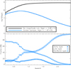 |
Fig. 3. Top panel: number of galaxies per redshift interval. The LSST golden selection cut is defined by mi < 25.3. Bottom panel: relative distribution of the broad types of the galaxies satisfying the LSST golden selection cut as a function of the redshift. |
We note that in the full simulation of the mock catalogue, dust extinction, photometric errors and use of 51 interpolated SEDs (instead of 6 main SEDs) are included. This comes to be small differences between the numbers from the curve labelled Zucca, derived from the full simulation and the results labelled Zucca of the simplified model presented in Fig. 2.
In order to take into account realistic uncertainties on the redshift, random errors were added to the true redshift zs. We studied four error models:
-
a Gaussian error with σ = 0.03 * (1 + zs),
-
a more realistic photo-z reconstruction using PDF distributions described in Sect. 3.1,
-
a photometric error improved by quality cuts on the BDT variable as described in Sect. 3.1.1, keeping 90 (BDT 90%) or 80% (BDT 80%) of the galaxies.
3. Photometric redshift reconstruction
To guarantee the cosmological capabilities of LSST, photo-z reconstruction quality requirements are provided in the LSST Science Collaboration et al. (2009). Statistical properties of the distribution of ez = (zs − zp)/(1 + zp) as a function of zp where zs denotes the spectro-z and zp denotes the photo-z, have to verify the following requirements:
-
the interquartile range (IQR) of ez is lower than 0.05 (the goal is lower than 0.02),
-
the fraction of outliers fout defined as the fraction of galaxies with ez > 0.15 is lower than 10%,
-
the bias b defined as the median value of ez is lower than 0.003.
We note that our Gaussian error model corresponds to IQR ≈ 0.04 as IQR ≈ 2 × 0.6745 × σ.
3.1. Method
The photo-z reconstruction is performed with a template fitting method presented in details in Gorecki et al. (2014). The SED library is made of 51 templates used for the photometry computation. We note that this step of the work is expected to be rather optimistic for LSST redshift reconstruction performance since our SED library completely represents the simulated observations. The method uses the prior proposed in Benítez (2000) to remove some degeneracies (mostly Lyman/Balmer breaks) based on magnitude distribution in the i-band. For each galaxy we had to compute a 3D-grid of χ2(z, T, EB − V) where the redshift z, the galaxy type T and the extinction from inner dust EB − V are the three parameters determined by the photo-z reconstruction code. The extinction follows the Cardelli et al. (1989) or Calzetti et al. (1994) law, depending on the galaxy type. We marginalised the χ2 grid over the two other parameters to get the marginalised 1D posterior probability density functions P(z), P(T) and P(EB − V). The redshift estimator can be chosen as  (value of the triplet that minimise the χ2 in the grid) or
  , value that maximises the posterior probability density function P(z). In this work we have used the latter one:
  . This code gives photo-z performances similar to other public codes (Ricol et al., in prep.) but allows us more freedom, in particular the possibility to compute our PDF functions.
3.1.1. Outliers rejection
The originality of the method is the outliers effective rejection with a machine learning technique based on the characteristics of the PDFs.
We have improved this technique in the present work. The Likelihood Ratio method presented in Gorecki et al. (2014) has been indeed replaced by a boosted decision tree (BDT) algorithm based on the same discriminant parameters but more robust and performant. The parameters used in the BDT are:
-
the number of peaks in the marginalised 1D posterior probability density functions denoted by Npk(θ), where θ is either z, T or EB − V,
-
when Npk > 1, the logarithm of the ratio between the height of the secondary peak over the primary peak in the 1D posterior probability density functions, denoted RL(θ),
-
when Npk > 1, the ratio of the probability associated with the secondary peak over the probability associated to the primary peak in the 1D posterior probability density functions, denoted by Rpk(θ)(the probability is taken proportional to the integral of the PDF between two minima either side),
-
the absolute difference between zpk and
 , denoted by
  ,
, -
the maximum value of log(ℒ) where ℒ is the likelihood,
-
the colours C = (u − g, g − r, r − i, i − z, z − y),
-
the photo-z value
 .
.
The BDT method is trained on an independent sample of 100 000 galaxies. The impact of the training sample (number of galaxies, completeness) has been studied in details in Gorecki et al. (2014) and shows no significant bias within reasonable statistics. After training, the BDT method provides a BDT value between −1 and 1 for each test sample galaxy, outliers having lower BDT values than good reconstructions. We can then apply a cut on this number.
The technics on photo-z reconstruction are continuously improved, see for instance Süveges et al. (2017), Cavuoti et al. (2017), Sadeh et al. (2016), Gomes et al. (2017), Pasquet et al. (2019). However, we do not expect significant changes in the main features of the reconstructed photo-z distributions and the impact of the LSS power spectrum reconstruction.
3.1.2. Fast photo-z computation
For a sake of computing time we have developed a fast photometric redshift reconstruction (hereafter FastPZ) tool that allows us to quickly compute the photo-z for each galaxy. The FastPZ tool is based on true photo-z distributions sorted in bins of true redshift, absolute magnitude and broad type. We used 121 bins in absolute magnitude M (from −24 to −12 with a step of 0.1), 3 bins in broad type BT (early, late or starburst) and 61 bins in redshift z (from zero to three with a step of 0.05) leading to a total of 21 780 bins. In each bin we simulated several thousands of photometric data, computed the photo-z for galaxies satisfying the LSST golden selection cut and constructed the P(zp − zs|M, BT, zs) distributions. For very low statistic bins we increased the number of galaxies in order to get reliable distributions.
The full method uses photometric information in the six filters, and is applicable to real data. In a simulation framework, the fluxes are first computed from the broad type, the absolute magnitude and the true redshift of each galaxy. The FastPZ method directly used the 3D (BT, zs) mapping to retrieve the reconstructed photo-z PDF from the broad type and the absolute magnitude of the galaxy. This method was able to compute ten million of photo-z’s in one second while it needed several hundreds of hours with the full method, resulting in a gain of CPU of about one million.
We have checked that performances of the FastPZ tool and the whole redshift reconstruction are very similar (Ricol et al., in prep.). Figure 4 presents the results of the FastPZ and the performances of the outliers rejection with the BDT method applied on our mock catalogue of ≈1.4 billion galaxies. The BDT cut value is tuned to keep a given percentage of the total number of galaxies.
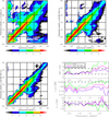 |
Fig. 4. Distribution of the photo-zzp as a function of the spectro-zzs. Top left panel: photo-z from the FastPZ method (see Sect. 3.1.2); top right panel: with the BDT 90% cut; bottom left panel: with the BDT 80% cut. The colour scale for the galaxy density is logarithmic. Bottom right panel: statistical properties of ez = (zs − zp)/(1 + zp) as a function of zp with (top panel) the interquartile range IQR of ez, (middle panel) fraction of outliers fout, defined by |ez|> 0.15, (bottom panel) bias b, defined as the median of ez. Green lines show the values obtained with the photo-z’s without any quality cut while the pink (purple) lines show the results with the photo-z satisfying BDT 90% (BDT 80%) cut. The dashed black lines correspond to the LSST requirements (plus the goal value in the IQR case). |
Figure 4 (top left) shows the density of photo-zzp as a function of the spectro-zzs. While most of the reconstructed redshifts lie close to the diagonal, the plane is almost filled by some “catastrophic” reconstructions, i.e. galaxies labelled as outliers. Nevertheless, the galaxy density is shown with a logarithmic colour scale, so at least one thousand times more galaxies lie in the diagonal area than in the green areas.
Figure 4 (top right and bottom left) shows the same distribution as previously, but after use of the BDT 90% or BDT 80% cut to reject outliers. Galaxies lying in the diagonal area are mostly unaffected while all the space above the diagonale is now almost completely cleared out. The part below the diagonal is much cleaner too. If the BDT cut is always efficient, it is particularly powerful at high redshift (zs > 1.5) where the number of galaxies with catastrophic redshift is reduced by at least two orders of magnitude.
The quality of the photo-z reconstruction is evaluated with the estimators used by the LSST collaboration. These statistical properties of ez = (zs − zp)/(1 + zp) are plotted as a function of the photo-z in Fig. 4 (bottom right). The LSST requirements are more or less satisfied by all the photo-z reconstructions up to zp ≈ 1.6. For higher redshifts, a BDT cut is mandatory, the IQR remains close the requirement and the bias varies significantly. We note that a similar degradation of the photo-z reconstruction performance is observed above z = 1.6−1.8 in the real data of the Hyper Suprime-Cam Subaru Strategic Program Data Release 1 Tanaka et al. (2018).
3.2. Error model statistics, selection functions and quality cuts
Selection functions are computed as the ratio between observed galaxy redshift distributions (spectroscopic, Gaussian, or photometric), satisfying the LSST golden selection cut, and the “true” redshift distribution of all galaxies (black line of Fig. 3). We do, of course, have to limit the magnitude when true galaxies are simulated. “No magnitude cut” means mi < 27, which should be close to the depth of the stacked images after the ten-year survey completion. Galaxies are simulated with absolute magnitude in the range [−24, −13]. This range is appropriate to our simulation as, even at the lower redshifts, the selection function remains below but close to one, so we simulate just enough, but not too many very faint galaxies.
The selection functions are shown in Fig. 5. The main shape, shown by the cyan line, directly reflects the LSST golden selection cut. The selection function with the Gaussian error model is very close to the one using spectro-z, but the ratio of the two functions exhibits an expected slight warp as the smoothing of a power-law-like distribution leads to a flattening of this distribution. Cases with photo-z error models are very different: the ratio between the selection function of any of the photo-z cases and the spectro-z case exhibits significant structures. Asymmetric ez distributions are responsible for these visible distorsions since they induce migration of galaxies from true redshift distribution into a distorted measured redshift distribution. It is particularly visible around z = 0.5 (see Fig. 6, top left). Difficulties in the photo-z reconstruction with asymmetric distributions around this redshift are rather generic, for instance it has been deeply studied by the SDSS collaboration Beck et al. (2016).
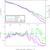 |
Fig. 5. Selection functions SF in the redshift range [0.2−2.45], using the various estimations of the redshift. Top panel: selection functions defined as the ratio between the number of galaxies in the catalogue (passing the LSST golden selection cut) and the number of simulated galaxies. The right axis gives the galaxy density d per Mpc−3. Bottom panel: ratio between the selection functions and the selection function in the spectroscopic case. |
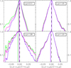 |
Fig. 6. Normalised histogram of ez = (zs − zp)/(1 + zp) for 4 bins in photo-z. The coloured vertical lines show the value of the bias for the 3 error models on the photo-z considered (see Fig. 5 for colour legend) while the dashed black line is the reference at 0. |
Additionally, catastrophic redshift reconstructions significantly affect the selection function at high redshift, let us say above z = 1.6. Indeed, a small fraction (a few percents) of the large low-redshift galaxy population can significantly contaminate (up to 30%) the much less populated regions at high redshift. The use of the BDT cut makes the selection function slightly smoother as the IQR, the bias and the number of catastrophic photo-z are significantly reduced. The cost is an additional decrease of the number of usable galaxies, from 2‰ to less than 1‰ at z = 2 for instance.
The origin of the bias is interesting. A residual bias can be corrected for only if it is attributed to a determination method that is known to systematically over or underestimate a measurement. It appears not to be the case here, as illustrated by Fig 6. The normalised histograms of ez have been plotted for 4 bins in redshift chosen for their various bias values (visible as the gap between the dashed black and the coloured vertical lines). The ez distributions have their maximum near zero, but when they are strongly asymmetric, the means differ significantly from the median. Here, applying global shifts to the photo-z distribution would be improper. Around zp = 0.51 or 1.89, the bias in the photo-z case is far beyond the requirements but the BDT cut significantly decreases the asymmetry of the ez distribution and the bias becomes marginally compatible with the requirements at the cost of a significant loss of galaxies. Contrarily, at zp = 1.05 or 1.20, the bias is small, close to the requirement, and the IQR and the fraction of outliers are satisfactory (see Fig. 4): there is clearly a systematic effect but it remains compatible with the requirements and the BDT cut is not able to improve the symmetry of the ez distributions.
3.3. Number density of galaxies
The redshift evolution of the galaxy number density (in Mpc−3), for galaxies satisfying the LSST golden selection cut, with and without BDT quality cut is shown in top panel of Fig. 5 (right vertical axis). Additionally, the average galaxy number density for few redshift ranges is given in Table 1. The impact of the error model on the galaxy density is driven by the BDT cut: 10 or 20% of the galaxies are lost with the BDT 90% or BDT 80% cuts, by definition. We notice the differences on the number of galaxies between the first two redshift bins, using Gaussian or photo-z redshifts: we retrieve the partial redistribution of the galaxies around z = 0.5, already seen in the shape of the selection functions, when photo-z are used.
Number of galaxies per arcmin2 per redshift range.
Table 2 gives the fraction of galaxies with relative redshift difference ez lower than some thresholds. The LSST requirement on the fractional photo-z error is 5% with a goal of 2%. Galaxies with a fractional photo-z error of 15% are considered as outliers. The three columns in Table 2 correspond to these three thresholds.
Fraction of galaxies fgal with |ez| = |zs − zp|/(1 + zp) lower than several thresholds for the three photometric error models.
4. Computation on the power spectra at different redshifts
Our aim is to quantify the impact of photometric redshifts on the LSS power spectrum P(k) and the BAO scale sA determination in LSST. We have thus chosen to use a Fourier Transform based procedure, which is a rather simple, robust, and well tested method to determine the LSS power spectrum. Other methods, such as direct computation of the two-point correlation function are often used when analysing observed galaxy catalogues, Szalay et al. (2003) or Anderson et al. (2012) for instance. These methods can indeed be better suited to real data, as they can more easily handle inhomogeneous sampling of space, for example blind spots due to bright stars, which require the use of masks, but more time consuming than FFT. Nevertheless, difficulties related to Fourier-space analysis can be overcome Beutler et al. (2016b).
Assuming a fiducial cosmology, galaxy angular positions and redshifts are converted into cartesian positions which are used to project the galaxies (weighted by the inverse of the selection function) into a 3D-grid nobs(r). There is a defect in this grid-FFT method. Cartesian grids are not well adapted to the spherical geometry and a clean definition of the redshift range. We have overcome this by the use of several grids, each set paving the spherical shell in a given redshift range, as described below.
A FFT is applied to compute the Fourier modes F(k) of the grid nobs(r) and the power spectrum of each normalised, mean subtracted galaxy number density grid:
![Mathematical equation: $$ \begin{aligned} F({\boldsymbol{k}}) = \mathrm{FFT} \left[ \frac{n_\mathrm{obs} ({\boldsymbol{r}})}{\bar{n}_\mathrm{obs} } - 1 \right], \quad P_{\rm obs}(k) = \langle |F({\boldsymbol{k}})|^2 \rangle . \end{aligned} $$](/articles/aa/full_html/2019/03/aa33732-18/aa33732-18-eq7.gif) (1)
(1)
The BAO scale is then extracted from the power spectrum through a fit of a damped sinusoid to the ratio of the observed power spectrum to a wiggle-less (no BAO) power spectrum (see Sect. 4.3).
4.1. Multiple grids covering a redshift range
First, the volume of universe covered by the simulated galaxy catalogue is organised as several sets of 3D-grids, each set covering a given redshift range. Euclidian (x, y, z) axes are defined with respect to the observer, with the Oz axis corresponding to the line of sight through the centre of the field. A given direction Ω = (θ, φ) is defined by two angles, θ being the angle with respect to Oz and φ the angle of the projection of Ω on the xOy plane with Ox axis.
The grid thicknesses are a compromise between a reasonably small redshift range, sufficient statistics and high enough volume to be sensitive to low k-values (kmin ∼ 0.005). The margin with respect to the initial BigCube limits must be sufficient to avoid artificial loss of galaxies, as the photo-z errors can be large, especially at high redshifts.
We have defined three sets of five grids each, centred at redshifts z = 0.5, 0.9, 1.3, each grid being subdivided into 8 × 8 × 8 Mpc3 cells. One grid is centred along the Euclidian z axis while the others are rotated by 40° in θ and scattered at 0, 90, 180, and 270° in φ. A 3D-view of the grids is drawn in Fig. 7: the initial BigCube is represented by the white box, the field-of-view by the grey area while grids are drawn in colours according to their redshift range.
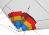 |
Fig. 7. Schematic view of the volumes used in the simulation. The black lines mark out the BigCube. The grey area shows the field of view of π sr which is filled by galaxies from z = 0.2 to z = 2.45. The five grids used to compute each power spectrum are drawn in blue, orange, or red according to their central redshift. |
Table 3 summarises the main characteristics of these three grid sets. After projection of the galaxy catalogue into the grids, each cell contains the number of galaxies with a position falling in it, weighted by the inverse of the selection function corresponding to the considered error model at the appropriate redshift.
Geometrical description of the grids used for the power spectrum computation and mean number of galaxies falling in one of the five grids in each set, with and without BDT cut.
Figure 8 shows the galaxy density contours of two slices through the centre of the z = 0.9 central grid. The (x, y) slice corresponds to the transverse plane and the (z, y) slice contains the line-of-sight Oz axis. While density contours are isotropic and small structures are well contrasted with spectro-z (left panels), features appear along the radial (redshift) direction and small structures have faded out with photo-z (here BDT 80%, right panels).
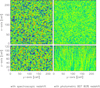 |
Fig. 8. Galaxy density contours in slices of the grid centred at z = 0.9. Top panel: transverse plane (y, x). Bottom panel: radial plane (y, z). Left panel: with spectro-z, right panel: with BDT 80% photo-z. Slices are eight co-moving Mpc thick (one cell) and go through the grid centre. |
4.2. Power spectra and noise estimation
We have computed power spectra Pobs(k) for each of the five redshift error models: spectroscopic redshifts (no-error), redshifts with gaussian error σz = 0.03(1 + z) and photo-z reconstruction without or with 90% or 80% BDT cut.
We also computed the shot noise contribution by simulation. A separate set of grids is filled by Poisson noise using the mean galaxy density at the redshift of each cell. Further steps – application of the error model on the redshift or selection function correction for instance – are then applied as for grids filled by galaxies. The power spectra of the shot noise grids PSN are flat and the shot noise contribution is properly approximated by a constant, as expected, which is determined with a small statistical uncertainty.
The shot noise subtracted power spectrum is defined by PD(k) = ⟨Pobs(k)⟩3D − grids − PSN, where the subscript D stands for damped. Indeed, the recovered power spectrum is damped due to redshift errors, compared to the underlying galaxy distribution power spectrum.
Theoretical (input) and recovered power spectra from simulated galaxy catalogues, at the three redshifts and for the five redshift error models, are shown in Fig. 9.
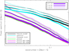 |
Fig. 9. Recovered power spectra PD(k) computed from the five grids centred at each redshift bin, after subtraction of the shot noise contribution. Black lines correspond to the theoretical (input) power spectra while other colours refer to the five redshift error models. The line thickness identifies the grids central redshift. Thickness increases with redshift. |
One can see the global decrease in amplitude at all scales when the redshift increases, by comparing for instance the theoretical shapes (black lines). It is related to the increasing growth factor with cosmic time. The power spectra recovered from catalogues with spectro-z for the three redshift ranges (cyan curves) follow the theoretical shapes at low k, but a moderate damping can be seen, starting around k = 0.1, which is mainly due to the sampling with 83 Mpc3 cells.
The damping of the power spectrum produced by the photometric redshift smearing is clearly visible when errors on redshift are introduced. The damping factor reaches a factor of approximately ten at the BAO scale, around 150 Mpc (k ≈ 0.04).
The BDT cut reduces the photo-z dispersion, so reduces the damping: the recovered power spectrum amplitude increases with more stringent BDT requirement. We note that the differences are tiny between the green, pink and purple medium thickness curves, as photo-z performance is already good around z = 0.9 without any BDT cut. The amplitude of the recovered spectra from the grids centred at z = 0.5 and z = 1.3 are more sensitive to the BDT cut.
The power spectra for the grids centred at z = 1.3 start to flatten at high k because they are not far from being shot noise dominated with an average of only two galaxies per cell (see Table 3). The statistical errors associated to the recovered power spectra are given by:
![Mathematical equation: $$ \begin{aligned} \sigma _{\rm P} (k)= \frac{2 \pi }{k \sqrt{V \delta _k}} \times \left[ P_\mathrm{D} (k) + P_{\mathrm{SN}} \right] \end{aligned} $$](/articles/aa/full_html/2019/03/aa33732-18/aa33732-18-eq8.gif) (2)
(2)
where V is the total volume of the grids in a given redshift range and δk is the sampling width in wave number. We have checked that the dispersion of the recovered power spectra from different mock catalogues do follow the above relation, although with limited number of catalogues, due to CPU and storage intensive computations needed to generate and analyse the catalogues.
The fractional statistical uncertainty on the recovered power spectrum σP/P(k) is plotted in Fig. 10. It depends naturally on the wave number k, but also on the redshift interval and on the redshift error model. One can distinguish two regimes from these curves: Firstly, the fractional power spectrum error σP/P(k) is dominated by the cosmic variance at low wave numbers (k < 0.015), for all of the five error models and all redshift intervals. It remains true with spectroscopic redshifts up to, at least, k ≈ 0.15. The cosmic variance contribution is larger for low redshift as the grids are smaller and it evolves as 1/k. Secondly, at medium or high wave numbers, the fractional statistical error σP/P(k) is dominated by the shot noise contribution. The lower limit in wave number for this regime depends on the redshift range.
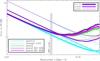 |
Fig. 10. Fractional statistical error σP/P(k) of the recovered power spectra PD in percent. Colours identify the different redshift error models, while the grid redshifts are distinguished by different line thicknesses. The light grey area shows the wave number corresponding to the BAO scale. |
The shot noise contribution is significantly lower when spectro-z are used. Indeed the shot noise levels, which depend on the mean galaxy density, are very similar for the spectroscopic, Gaussian and photometric cases. However, their relative values with respect to the power spectrum PD(k) increase significantly as PD(k) are damped due to radial smearing (Gaussian or photo-z error models). We note that even with spectro-z, for the 3D-grids centred at z = 1.3, the relative error contribution flattens at k ≈ 0.2, as the shot noise starts to overwhelm the LSS power spectrum.
In summary, we can expect a more accurate BAO scale determination from the grids centred at z = 0.9, compared to the grids centred at z = 0.5 and z = 1.3. The precision on the recovered power spectrum is limited by the cosmic variance at low redshift (z = 0.5) and by the shot noise at high redshift (z = 1.3). We note that non-linearities will also soften the oscillations above k ≈ 0.1 Mpc−1.
4.3. Extraction of the BAO scale
The baryon acoustic oscillations are subdominant with respect to the global matter power spectrum shape, as they are hard to see even on theoretical curves (black lines in Fig. 9). Thereby, the power spectrum, damped by any feature affecting the data or the computation method, follows a global shape with the small superimposed oscillations.
We do not want to assume any shape of the damping induced by the smearing produced by photo-z errors. So we cannot use an analytical model as it is done for Gaussian error model Glazebrook & Blake (2005). The appendix contains the description of the procedure that we have developed to estimate the smooth, wiggle-less, power spectrum from the observed one. The oscillating component in the spectrum is extracted, through the fitting of a damped sinusoid, similar to the wiggle-only method Glazebrook & Blake (2005) where the amplitude, the damping scale and the oscillation scale are left as free parameters.
As mentioned in Sect. 2, we have used a simple model in this simulation, ignoring non-linear effects or bias on the LSS power spectrum and mock galaxy catalogue generation. Indeed, non-linear clustering affects the power spectrum, leading in particular to a damping of the BAOs features at small scales Crocce & Scoccimarro (2008), Rasera et al. (2014), Obuljen et al. (2017) or Seo & Eisenstein (2007). In order to limit over-estimating LSST capability to recover the BAO scale, we have restricted the k-range used to extract the oscillating component in the power spectrum and to determine the BAO scale sA. We have used two k-ranges, a very conservative one in which only k ≤ 0.1 h Mpc−1 (i.e. k ≤ 0.07 Mpc−1) have been kept, and a second one, using wave modes up to k ≤ 0.15 h Mpc−1 (i.e. k ≤ 0.1 Mpc−1). Indeed the impact of non-linear clustering for low k-modes (k ≤ 0.1 h Mpc−1) can be safely neglected. However, as one can see for instance from Rasera et al. (2014), the damping of the BAO features due to non-linear clustering is limited up to 0.15 h Mpc−1, specially at higher redshifts (z ≥ 1), which is more the focus of this work. The comparison of the reconstructed BAO scale error from these two k-ranges gives an indication of the amount of information in larger k-modes for different redshift bins.
For illustration purpose, we show the oscillating component of the LSS power spectrum in the Fourier space, as well as the fitted damped sinusoid, for the redshift z = 0.9 on Fig. 11. The estimated errors on sA are gathered in Fig. 12 for the two tested k-ranges. In agreement with previous considerations, results obtained for 3D-grids centred at z = 0.9 are more precise than results obtained from 3D-grids centred at lower or higher redshifts. The results are two or three times worse if the k-modes between 0.07 and 0.1 Mpc−1 are removed. Indeed the loss of half of the second oscillation impacts the ability to precisely recover the BAO scale. Nevertheless this loss does not suppress it completely, as the error remains below 5% in all cases.
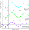 |
Fig. 11. Recovered oscillation part of the power spectra in Fourier space for the grids centred at z = 0.9 considering, from top to bottom panel, spectro-z, photo-z without and with BDT 80% cut. The coloured lines are the fitted oscillations using the simple “wiggle only” description. The BAO scale is at the first intersection between this fitted damped sinusoid and the horizontal black line. The expected value of kA from the fiducial Planck 2015 ΛCDM model (0.0417 Mpc−1) is shown by the vertical line. |
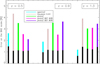 |
Fig. 12. Relative errors on the BAO scale fitted from the power spectra for each redshift and each error model. The black bars are the results using the k-range [0.03−0.1] Mpc−1 while the colour bars are the results using the k-range [0.02−0.07] Mpc−1. |
In some cases in particular, the errors are probably underestimated, preventing proper estimation of the impact of the BDT cut on the recovery of the BAO scale. Indeed, the reduced χ2 are reasonably close to one when spectro-z are used and for all error models for grids centred at z = 0.9 and z = 1.3. But the reduced χ2 ranges from five to six when the fit is performed from grids centred at z = 0.5 with Gaussian or photometric error on the redshift. We interpret this as a suggestion that another component in the error computation related to the error on the redshift should be included. This component is mainly hidden by the shot noise at higher redshifts. It is due to the redshift dispersion and not to the bias or the presence of outliers as the χ2’s are similar with the Gaussian error model (with no bias and virtually no outlier) and with the photo-z error model.
5. Interpretation and discussion
In this section we try to explain some of the general behaviours that we have observed using the full simulation in the previous section. We then describe how we used a simple simulation tool implementing these effects to get BAO scale determination uncertainty in a LSST-like survey, compared to a fiducial spectroscopic survey.
The use of photo-z induces two main effects on the galaxy distribution. A first one is the smearing along the radial direction, due to reconstructed redshift uncertainties, and a second one is the presence of outliers, due to catastrophic redshifts. We can write the observed galaxy number densities nobs(r) along the line of sight r from which the underlying LSS matter power spectrum is computed as
 (3)
(3)
where  (resp. nout) denotes galaxy population with reasonable photo-z (resp. outliers). Introducing the outlier fraction fout, we have the following relations between the different average number densities:
 (4)
(4)
The observed matter distribution power spectrum is computed from the galaxy number density field renormalised by the average density
![Mathematical equation: $$ \begin{aligned} P_{\rm obs}(k):\;\mathrm{FFT} \left[ n_{\rm obs}({\boldsymbol{r}}) / \bar{n}_{\rm obs} - 1 \right]. \end{aligned} $$](/articles/aa/full_html/2019/03/aa33732-18/aa33732-18-eq12.gif) (5)
(5)
Neglecting the correlation between galaxies with correctly reconstructed redshifts and outliers, the observed power spectrum can be written as
 (6)
(6)
The different terms of this equation correspond to:
-
The Pg(k)×η(k) term corresponds to the power spectrum of the galaxy number density field radially smeared due to photo-z errors, leading to a damping of the power spectrum (0 < η(k) ≤ 1). η(k) follows a scaling law: η(k) = f(k × σR) with σR the standard deviation of the smearing along the radial direction as described in Blake & Glazebrook (2003).
-
Outliers correspond to galaxies from different redshifts shuffled to a large extent, so Pout(k)≲Pg(k); they contribute to the overall noise in the observed galaxy power spectrum. However, the outliers contribution would be negligible in most cases, as long as fout < 10%.
-
PSN is the combined shot noise power spectrum from the two populations
 (7)
(7)
We have computed the damping function η(k), corresponding to the ratio of the recovered power spectrum to the input power spectrum, for different levels of smearing along the radial direction. The left panel of Fig. 13 shows the damping function η(k) for four values of the standard deviation σR = 50, 75, 100, 150 Mpc of Gaussian smearing along the radial direction. The damping function very closely follows a scaling law, η(k) = f(k/k0) where  , as shown in Fig. 13. The damping function is well represented by the analytic function
 (8)
(8)
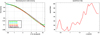 |
Fig. 13. Left panel: damping function η(k) for four values of σR = 50, 75, 100, 150 Mpc (colour curves) and its analytical approximate shape |
We have also plotted  as a function of redshift on the right panel of Fig. 13, using the redshift dependent σpz(z) from full photo-z reconstruction of Sect. 3 with BDT 90% selection cut.
We have carried out a study of the BAO scale reconstruction uncertainty using a toy program where the observed galaxy power spectrum and associated errors are computed using the expressions given above. The galaxy power spectrum has been damped using a redshift dependent radial smearing σR(z), as represented by the IQR variable in Fig. 4, and a fixed value of 5% for the outlier fraction. We note that σR(z) is very irregular, as is the IQR in Fig. 4; this variability is not due to a lack of statistics but to galaxies spectra features seen by the photo-z method. We have used redshift dependent galaxy number density following the values obtained in our full simulation, slightly below the ones shown in Fig. 2. We computed the ratio of the observed power spectrum to a theoretical power spectrum without BAO oscillations R(k) = (Pobs(k)−PSN)/(Pno − osc(k)*η(k)). The BAO scale sA is then determined by fitting a damped sinus function Aexp(k/kd)sin(sA k) to the ratio R(k), with three free parameters: A, kd, sA, over the restricted k-range 0.03 ≤ k ≤ 0.1 Mpc−1, equivalent to 0.04 ≤ k ≤ 0.15 h Mpc−1. A constant quadratic error of 0.4% has been included to compensate partially for the simplicity of this fitting method. The increase of the uncertainty due to photo-z smearing is however marginally sensitive to the fitting procedure. The error is determined from the distribution of reconstructed BAO scales sA.
The survey volumes given in Table 3 correspond to a survey of slightly less than 4000 deg2. Using our toy program and for Ωsurv = 4000 deg2, we obtain a BAO scale uncertainty σsA of 1.9 Mpc (≈1.3%) and 2.2 Mpc (≈1.5%) for spectro-z and photo-z, with kmax = 0.1 h Mpc−1 for the redshift bin centred at z = 0.9, in reasonable agreement with the error bars represented in Fig. 12. It should be stressed that the uncertainties given by the toy program should be considered as a lower limit of the true error bars, as the galaxy power spectrum and the one without BAO oscillations, as well as the damping function η(k) are supposed to be perfectly known. However, the comparison between spectro-z and photo-z remains meaningful.
We have used this toy program to compute σsA for an LSST-like survey and an effective survey area Ωsurv = 10 000 deg2, in six redshift bins in the range [0.4−2.2]. The results are summarised in Table 4, where one can see the increase of the error on the BAO scale due to photo-z. Despite high galaxy number density, the relatively large value of σsA around z ∼ 0.5 can be explained by the more limited survey volume and larger photo-z dispersions, which has an even larger impact due to smaller Hubble parameter H(z). The BAO scale would be rather well constrained by the LSST survey in the redshift range 0.7 ≲ z ≲ 1.6, thanks to good photo-z reconstruction and large galaxy number densities. The degradation of BAO scale determination is visible for redshifts above z ∼ 1.6 and even more clearly above z ∼ 2, where σsA is increased by a factor of approximately four in the case of photo-z, compared to a full spectro-z.
BAO scale determination relative uncertainty σsA for different redshift ranges, for an ideal survey (left), for an LSST-like photometric survey (middle), and for a fiducial spectroscopic survey (right) with Ωsurv = 10 000 deg2.
We have also included forecasts of σsA for a fiducial spectroscopic survey with realistic galaxy number densities in Table 4. Spectroscopic surveys naturally have a significantly lower galaxy number densities than photometric surveys which limit their statistical power to map the LSS. To determine the galaxy number density for our fiducial spectroscopic survey, we have used the foreseen number of objects in the DESI survey Aghamousa et al. (2016). They expect to reach ∼1625 objects per deg2 up to redshift ∼2.1, by considering LRG’s up to redshift 1 (0.4 < z < 1.0), ELG’s in the redshift range 0.6 < z < 1.6 and QSO’s up to redshift z ∼ 2.1. This galaxy density is about 75 times less than the one expected for LSST (≳125 000 per deg2). However, to be conservative, we have applied a factor 50 to the LSST galaxy number densities for the first four redshift bins, up to z < 1.6, and a factor of 30 for the last two redshift bins 1.6 < z < 2.2 to obtain the galaxy densities n̄gal for computing forecasts for our fiducial spectroscopic survey.
The amount of information available in the high k-modes can be evaluated by comparing the gain in the BAO scale precision by extending the k-range in the fit, in other words, by fixing kmax to 0.1 instead of 0.07 Mpc−1. Such an extension would lead to a decrease of the relative uncertainty σsA by almost a factor of two. It is probably slightly less if the natural smoothing produced by non-linear effects is taken into account. The gain is more limited at higher redshifts as the shot noise becomes dominant. The ability to properly model the non-linear part of the LSS power spectrum may give access to a still larger k-range. A hint of the improvement is given by the last column, for a fiducial spectroscopic survey, with oscillations fitted up to k = 0.2 Mpc−1. We note that such small scales are mainly removed, hidden by the shot noise, if photo-z are used (see Fig. 10).
Comparing the columns of Table 4 shows the robustness of the BAO scale as a standard ruler, even if a relatively small fraction of the galaxies is used or if the redshift suffers from some dispersion. This parameter is statistically mostly immune to these defects below z ≈ 1.5. Nevertheless, the LSS power spectrum is significantly damped if photo-z are used. Thus, using the whole shape, and not only the BAO scale, would require a very precise knowledge of the photo-z properties at the origin of the damping function η(k), while it is more directly provided by spectro-z surveys.
Here, only the isotropic BAO scale has been considered. However, we keep in mind that the BAO probe is more powerful in spectroscopic surveys, as they will be able to determine the BAO scale in the transverse and radial directions independently, and to measure the redshift space distortions. LSST, on the other hand, will mostly be sensitive to the transverse BAO scale due to photo-z smearing.
6. Conclusion and perspectives
The determination of accurate photometric redshifts of galaxies for redshifts up to at least two, is one the main challenges of the LSST survey. We have evaluated the impact of realistic photo-z uncertainties on the LSS power spectrum and the BAO scale uncertainty. The number density of usable galaxies and its evolution with redshift is one of the main parameters with major impact on cosmology with LSST. We have determined the expected galaxy number density in the LSST survey, which decreases from ∼0.015 Mpc−3 at redshift z ∼ 1 to ∼0.0015 Mpc−3 at redshift z ∼ 1 and associated photo-z errors. We have shown that LSST should be able to recover the BAO scale with few percents uncertainty up to redshift z ≲ 1.5.
Around z = 1, photo-z are accurate, with low bias and there is a small fraction of outliers. Therefore, LSST should be able to map accurately the galaxy distribution at this crucial stage of the history of the Universe, when the dark energy starts to dominate over matter. The redshift of closer or more distant galaxies is less accurately measured in LSST, due to degeneracies between redshift and galaxy type. At low redshifts, the use of additional information like a BDT cut is helpful, leaving enough galaxies to properly compute the matter power spectrum and extract the BAO scale. At high redshifts (z ≳ 1.5−2), the observed galaxy number density is small and cannot compensate any more the photo-z smearing and the BAO signal is mainly washed out. Our studies indicate that LSST will be able to recover with precision the BAO scale up to z ≈ 1.5, with a photo-z reconstruction performances within requirements, confirming previous studies, for example Zhan & Tyson (2018). However, our study also shows that previous conclusions were rather optimistic regarding higher redshifts, as the recovered LSS power spectrum suffers larger uncertainties, due to the combination of a lower galaxy number density and poorer photo-z reconstruction.
Using spherical shells and spherical harmonic transform instead of Euclidian grids and Fourier transform is better suited to the analysis of galaxy surveys with large sky coverage. In addition, the theoretical framework for LSS analysis with spherical shells has been extensively developed in recent years, for instance Bonvin & Durrer (2011), Lanusse et al. (2015), and Campagne et al. (2017). We plan to carry out a study of the impact of photo-z with separate determination of the radial and transverse BAO scales using spherical shells. At low redshift, especially around z ∼ 0.5, the LSS power spectrum uncertainty is not limited by shot noise in LSST, but suffers from photo-z spread and outliers. Identifying a population of galaxies with reliable photo-z at low redshifts would be another useful follow-up study.
Acknowledgments
Authors thanks the DESC Large-Scale Structures working group, especially D. Alonso and A. Slosar, for their useful comments. Authors thanks M. Moneuse for fruitful discussions and uses of CAMEL, even if the cosmological parameters part exceeds the scope of this paper.
References
- Abbott, T. M. C., Abdalla, F. B., Alarcon, A., et al. 2019, MNRAS, in press [arXiv:1712.06209] [Google Scholar]
- Abrahamse, A., Knox, L., Schmidt, S., et al. 2011, ApJ, 734, 36 [NASA ADS] [CrossRef] [Google Scholar]
- Aghamousa, A., Aguilar, J., Ahlen, S., et al. 2016, ArXiv e-prints [arXiv:1611.00036] [Google Scholar]
- Alam, S., Ho, S., Satpathy, S., et al. 2017, MNRAS, 470, 2617 [NASA ADS] [CrossRef] [Google Scholar]
- Alonso, D., Bellini, E., Ferreira, P. G., & Zumalacárregui, M. 2017, Phys. Rev. D, 95, 063502 [NASA ADS] [CrossRef] [Google Scholar]
- Anderson, L., Aubourg, E., Bailey, S., et al. 2012, MNRAS, 427, 3435 [Google Scholar]
- Aubourg, É., Bailey, S., Bautista, J. E., et al. 2015, Phys. Rev. D, 92, 123516 [NASA ADS] [CrossRef] [Google Scholar]
- Awan, H., Gawiser, E., Kurczynski, P., et al. 2016, ApJ, 829, 50 [NASA ADS] [CrossRef] [Google Scholar]
- Beck, R., Dobos, L., Budavári, T., Szalay, A. S., & Csabai, I. 2016, MNRAS, 460, 1371 [NASA ADS] [CrossRef] [Google Scholar]
- Benítez, N. 2000, ApJ, 536, 571 [NASA ADS] [CrossRef] [Google Scholar]
- Beutler, F., Blake, C., Koda, J., et al. 2016a, MNRAS, 455, 3230 [NASA ADS] [CrossRef] [Google Scholar]
- Beutler, F., Seo, H.-J., Saito, S., et al. 2016b, MNRAS, 466, 2242 [Google Scholar]
- Blake, C., & Glazebrook, K. 2003, ApJ, 594, 665 [NASA ADS] [CrossRef] [Google Scholar]
- Blake, C., Kazin, E. A., Beutler, F., et al. 2011, MNRAS, 418, 1707 [NASA ADS] [CrossRef] [MathSciNet] [Google Scholar]
- Bonvin, C., & Durrer, R. 2011, Phys. Rev. D, 84, 063505 [NASA ADS] [CrossRef] [Google Scholar]
- Calzetti, D., Kinney, A. L., & Storchi-Bergmann, T. 1994, ApJ, 429, 582 [NASA ADS] [CrossRef] [Google Scholar]
- Campagne, J. E., Neveu, J., & Plaszczynski, S. 2017, A&A, 602, A72 [NASA ADS] [CrossRef] [EDP Sciences] [Google Scholar]
- Cardelli, J. A., Clayton, G. C., & Mathis, J. S. 1989, ApJ, 345, 245 [NASA ADS] [CrossRef] [Google Scholar]
- Cavuoti, S., Tortora, C., Brescia, M., et al. 2017, MNRAS, 466, 2039 [NASA ADS] [CrossRef] [Google Scholar]
- Chang, C., Jarvis, M., Jain, B., et al. 2013, MNRAS, 434, 2121 [NASA ADS] [CrossRef] [Google Scholar]
- Coleman, G. D., Wu, C. C., & Weedman, D. W. 1980, ApJS, 43, 393 [NASA ADS] [CrossRef] [Google Scholar]
- Crocce, M., & Scoccimarro, R. 2008, Phys. Rev. D, 77, 023533 [NASA ADS] [CrossRef] [Google Scholar]
- Crocce, M., Ross, A. J., Sevilla-Noarbe, I., et al. 2019, MNRAS, 482, 2807 [NASA ADS] [CrossRef] [Google Scholar]
- Dahlen, T., Mobasher, B., Somerville, R. S., et al. 2005, ApJ, 631, 126 [NASA ADS] [CrossRef] [Google Scholar]
- Dawson, K. S., Schlegel, D. J., Ahn, C. P., et al. 2013, AJ, 145, 10 [Google Scholar]
- Drinkwater, M. J., Jurek, R. J., Blake, C., et al. 2010, MNRAS, 401, 1429 [Google Scholar]
- Eisenstein, D. J., & Hu, W. 1998, ApJ, 496, 605 [NASA ADS] [CrossRef] [Google Scholar]
- Glazebrook, K., & Blake, C. 2005, ApJ, 631, 1 [NASA ADS] [CrossRef] [Google Scholar]
- Gomes, Z., Jarvis, M. J., Almosallam, I. A., & Roberts, S. J. 2017, MNRAS, 475, 331 [Google Scholar]
- Gorecki, A., Abate, A., Ansari, R., et al. 2014, A&A, 561, A128 [NASA ADS] [CrossRef] [EDP Sciences] [Google Scholar]
- Graham, M. L., Connolly, A. J., Ivezić, Ž., et al. 2018, AJ, 155, 1 [NASA ADS] [CrossRef] [Google Scholar]
- Jones, D. M., & Heavens, A. F. 2019, MNRAS, 483, 2487 [NASA ADS] [CrossRef] [Google Scholar]
- Kinney, A. L., Calzetti, D., Bohlin, R. C., et al. 1996, ApJ, 467, 38 [NASA ADS] [CrossRef] [Google Scholar]
- Lanusse, F., Rassat, A., & Starck, J. L. 2015, A&A, 578, A10 [NASA ADS] [CrossRef] [EDP Sciences] [Google Scholar]
- Laureijs, R., Amiaux, J., Arduini, S., et al. 2011, ArXiv e-prints [arXiv:1110.3193] [Google Scholar]
- Lesgourgues, J. 2011, ArXiv e-prints [arXiv:1104.2932] [Google Scholar]
- Levi, M., Bebek, C., Beers, T., et al. 2013, ArXiv e-prints [arXiv:1308.0847] [Google Scholar]
- LSST Science Collaboration, Abell, P. A., Allison, J., et al. 2009, ArXiv e-prints [arXiv:0912.0201] [Google Scholar]
- Mandelbaum, R., Miyatake, H., Hamana, T., et al. 2018, PASJ, 70, S25 [NASA ADS] [CrossRef] [Google Scholar]
- Medezinski, E., Oguri, M., Nishizawa, A. J., et al. 2018, PASJ, 70, 30 [NASA ADS] [Google Scholar]
- Obuljen, A., Villaescusa-Navarro, F., Castorina, E., & Viel, M. 2017, JCAP, 2017, 012 [CrossRef] [Google Scholar]
- Pasquet, J., Bertin, E., Treyer, M., Arnouts, S., & Fouchez, D. 2019, A&A, 621, A26 [NASA ADS] [CrossRef] [EDP Sciences] [Google Scholar]
- Planck Collaboration XIII. 2016, A&A, 594, A13 [NASA ADS] [CrossRef] [EDP Sciences] [Google Scholar]
- Ramos, B. H. F., Pellegrini, P. S., Benoist, C., et al. 2011, AJ, 142, 41 [NASA ADS] [CrossRef] [Google Scholar]
- Rasera, Y., Corasaniti, P. S., Alimi, J. M., et al. 2014, MNRAS, 440, 1420 [NASA ADS] [CrossRef] [Google Scholar]
- Sadeh, I., Abdalla, F. B., & Lahav, O. 2016, PASP, 128, 104502 [NASA ADS] [CrossRef] [Google Scholar]
- Salazar-Albornoz, S., Sánchez, A. G., Grieb, J. N., et al. 2017, MNRAS, 468, 2938 [NASA ADS] [CrossRef] [Google Scholar]
- Seo, H.-J., & Eisenstein, D. J. 2007, ApJ, 665, 14 [NASA ADS] [CrossRef] [Google Scholar]
- Süveges, M., Fotopoulou, S., Coupon, J., et al. 2017, in Astroinformatics, eds. M. Brescia, S. G. Djorgovski, E. D. Feigelson, G. Longo, & S. Cavuoti, IAU Symp., 325, 39 [NASA ADS] [Google Scholar]
- Szalay, A. S., Jain, B., Matsubara, T., et al. 2003, ApJ, 591, 1 [NASA ADS] [CrossRef] [Google Scholar]
- Tanaka, M., Coupon, J., Hsieh, B.-C., et al. 2018, PASJ, 70, S9 [NASA ADS] [CrossRef] [Google Scholar]
- Zhan, H., & Tyson, J. A. 2018, Rep. Prog. Phys., 81, 066901 [NASA ADS] [CrossRef] [Google Scholar]
- Zhan, H., Knox, L., & Tyson, J. A. 2009, ApJ, 690, 923 [NASA ADS] [CrossRef] [Google Scholar]
- Zucca, E., Bardelli, S., Bolzonella, M., et al. 2009, A&A, 508, 1217 [NASA ADS] [CrossRef] [EDP Sciences] [Google Scholar]
Appendix A: Fit of the global shape of a power spectrum
The oscillating spectrum Pwiggle is fitted by the usual wiggle only method, which aims at recovering the BAO scale sA.
The polynomial description of the global shape is determined as follows:
-
computing abscissas of the inflexion points where no contribution of baryonic oscillation is expected – they depend on the assumed value of the BAO scale,
-
deriving from data the ordinates of these points by averaging the power spectrum around these abscissas,
-
fitting this set of inflexion points by a polynomial of fifth degree.
This method is illustrated by Fig. A.1. We have used power spectra weighted by the square of the spatial wave number (P(k)×k2) to enhance the readability. The baseline derived by this method is smooth by construction and adapt itself to include all kinds of damping.
This method has been validated with results obtained from grids filled with galaxies derived from matter distribution unaffected by baryonic oscillations. Such a power spectrum, with baryons but without baryonic oscillation, is available in the Eisenstein approximation Eisenstein & Hu (1998).
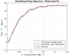 |
Fig. A.1. Example of a power spectrum and its fitted baseline. The initial power spectrum is drawn in black, the inflexion points are indicated by the blue crosses and the red curve is the result of the fit, providing the global shape of the input power spectrum. |
All Tables
Fraction of galaxies fgal with |ez| = |zs − zp|/(1 + zp) lower than several thresholds for the three photometric error models.
Geometrical description of the grids used for the power spectrum computation and mean number of galaxies falling in one of the five grids in each set, with and without BDT cut.
BAO scale determination relative uncertainty σsA for different redshift ranges, for an ideal survey (left), for an LSST-like photometric survey (middle), and for a fiducial spectroscopic survey (right) with Ωsurv = 10 000 deg2.
All Figures
|
Fig. 1. Graphic representation of the main steps of the simulation chain, from cosmological parameters up to the BAO scale measurement. |
| In the text | |
|
Fig. 2. Left panel: expected galaxy surface density as a function of the i-band magnitude limit: comparison of LSST Science Collaboration et al. (2009) extrapolation, numbers derived from the Dahlen et al. (2005) and Zucca et al. (2009) LFs parameters. Right panel: number of galaxies per Mpc3 as a function of redshift, for the LSST golden selection cut from Dahlen et al. (2005) and Zucca et al. (2009) LFs. Purple squares show results obtained with the Zucca et al. (2009) numbers, orange triangles show results obtained with the Dahlen et al. (2005) ones. |
| In the text | |
|
Fig. 3. Top panel: number of galaxies per redshift interval. The LSST golden selection cut is defined by mi < 25.3. Bottom panel: relative distribution of the broad types of the galaxies satisfying the LSST golden selection cut as a function of the redshift. |
| In the text | |
|
Fig. 4. Distribution of the photo-zzp as a function of the spectro-zzs. Top left panel: photo-z from the FastPZ method (see Sect. 3.1.2); top right panel: with the BDT 90% cut; bottom left panel: with the BDT 80% cut. The colour scale for the galaxy density is logarithmic. Bottom right panel: statistical properties of ez = (zs − zp)/(1 + zp) as a function of zp with (top panel) the interquartile range IQR of ez, (middle panel) fraction of outliers fout, defined by |ez|> 0.15, (bottom panel) bias b, defined as the median of ez. Green lines show the values obtained with the photo-z’s without any quality cut while the pink (purple) lines show the results with the photo-z satisfying BDT 90% (BDT 80%) cut. The dashed black lines correspond to the LSST requirements (plus the goal value in the IQR case). |
| In the text | |
|
Fig. 5. Selection functions SF in the redshift range [0.2−2.45], using the various estimations of the redshift. Top panel: selection functions defined as the ratio between the number of galaxies in the catalogue (passing the LSST golden selection cut) and the number of simulated galaxies. The right axis gives the galaxy density d per Mpc−3. Bottom panel: ratio between the selection functions and the selection function in the spectroscopic case. |
| In the text | |
|
Fig. 6. Normalised histogram of ez = (zs − zp)/(1 + zp) for 4 bins in photo-z. The coloured vertical lines show the value of the bias for the 3 error models on the photo-z considered (see Fig. 5 for colour legend) while the dashed black line is the reference at 0. |
| In the text | |
|
Fig. 7. Schematic view of the volumes used in the simulation. The black lines mark out the BigCube. The grey area shows the field of view of π sr which is filled by galaxies from z = 0.2 to z = 2.45. The five grids used to compute each power spectrum are drawn in blue, orange, or red according to their central redshift. |
| In the text | |
|
Fig. 8. Galaxy density contours in slices of the grid centred at z = 0.9. Top panel: transverse plane (y, x). Bottom panel: radial plane (y, z). Left panel: with spectro-z, right panel: with BDT 80% photo-z. Slices are eight co-moving Mpc thick (one cell) and go through the grid centre. |
| In the text | |
|
Fig. 9. Recovered power spectra PD(k) computed from the five grids centred at each redshift bin, after subtraction of the shot noise contribution. Black lines correspond to the theoretical (input) power spectra while other colours refer to the five redshift error models. The line thickness identifies the grids central redshift. Thickness increases with redshift. |
| In the text | |
|
Fig. 10. Fractional statistical error σP/P(k) of the recovered power spectra PD in percent. Colours identify the different redshift error models, while the grid redshifts are distinguished by different line thicknesses. The light grey area shows the wave number corresponding to the BAO scale. |
| In the text | |
|
Fig. 11. Recovered oscillation part of the power spectra in Fourier space for the grids centred at z = 0.9 considering, from top to bottom panel, spectro-z, photo-z without and with BDT 80% cut. The coloured lines are the fitted oscillations using the simple “wiggle only” description. The BAO scale is at the first intersection between this fitted damped sinusoid and the horizontal black line. The expected value of kA from the fiducial Planck 2015 ΛCDM model (0.0417 Mpc−1) is shown by the vertical line. |
| In the text | |
|
Fig. 12. Relative errors on the BAO scale fitted from the power spectra for each redshift and each error model. The black bars are the results using the k-range [0.03−0.1] Mpc−1 while the colour bars are the results using the k-range [0.02−0.07] Mpc−1. |
| In the text | |
|
Fig. 13. Left panel: damping function η(k) for four values of σR = 50, 75, 100, 150 Mpc (colour curves) and its analytical approximate shape |
| In the text | |
|
Fig. A.1. Example of a power spectrum and its fitted baseline. The initial power spectrum is drawn in black, the inflexion points are indicated by the blue crosses and the red curve is the result of the fit, providing the global shape of the input power spectrum. |
| In the text | |
Current usage metrics show cumulative count of Article Views (full-text article views including HTML views, PDF and ePub downloads, according to the available data) and Abstracts Views on Vision4Press platform.
Data correspond to usage on the plateform after 2015. The current usage metrics is available 48-96 hours after online publication and is updated daily on week days.
Initial download of the metrics may take a while.