| Issue |
A&A
Volume 620, December 2018
|
|
|---|---|---|
| Article Number | A157 | |
| Number of page(s) | 15 | |
| Section | Planets and planetary systems | |
| DOI | https://doi.org/10.1051/0004-6361/201833855 | |
| Published online | 12 December 2018 | |
Dynamics of multiple protoplanets embedded in gas and pebble discs and its dependence on Σ and ν parameters
1
Institute of Astronomy, Charles University, Prague,
V Holešovičkách 2,
18000 Prague 8, Czech Republic
e-mail: mira@sirrah.troja.mff.cuni.cz
2
Department of Space Studies, Southwest Research Institute,
1050 Walnut St., Suite 300, Boulder,
CO 80302, USA
3
Lund Observatory, Department of Astronomy and Theoretical Physics, Lund University,
Box 43,
22100 Lund, Sweden
Received:
13
July
2018
Accepted:
3
October
2018
Protoplanets of super-Earth size may get trapped in convergence zones for planetary migration and form gas giants there. These growing planets undergo accretion heating, which triggers a hot-trail effect that can reverse migration directions, increase planetary eccentricities, and prevent resonant captures of migrating planets. In this work, we study populations of embryos that are accreting pebbles under different conditions, by changing the surface density, viscosity, pebble flux, mass, and the number of protoplanets. For modelling, we used the FARGO-THORIN two-dimensional (2D) hydrocode, which incorporates a pebble disc as a second pressure-less fluid, the coupling between the gas and pebbles, and the flux-limited diffusion approximation for radiative transfer. We find that massive embryos embedded in a disc with high surface density (Σ = 990 g cm−2 at 5.2 au) undergo numerous “unsuccessful” two-body encounters that do not lead to a merger. Only when a third protoplanet arrives in the convergence zone do three-body encounters lead to mergers. For a low-viscosity disc (ν = 5 × 1013 cm2 s−1), a massive co-orbital is a possible outcome, for which a pebble isolation develops and the co-orbital is further stabilised. For more massive protoplanets (5 M⊕), the convergence radius is located further out, in the ice-giant zone. After a series of encounters, there is an evolution driven by a dynamical torque of a tadpole region, which is systematically repeated several times until the co-orbital configuration is disrupted and planets merge. This may be a way to solve the problem that co-orbitals often form in simulations but they are not observed in nature. In contrast, the joint evolution of 120 low-mass protoplanets (0.1 M⊕) reveals completely different dynamics. The evolution is no longer smooth, but rather a random walk. This is because the spiral arms, developed in the gas disc due to Lindblad resonances, overlap with each other and affect not only a single protoplanet but several in the surrounding area. Our hydrodynamical simulations may have important implications for N-body simulations of planetary migration that use simplified torque prescriptions and are thus unable to capture protoplanet dynamics in its full glory.
Key words: hydrodynamics / protoplanetary discs / planet-disc interactions / planets and satellites: formation
© ESO 2018
1 Introduction
The way a giant planet core forms is a key to understand the evolution of the solar system, and exoplanetary systems as well. It is believed that gas giants, and possibly (some subset of) the super-Earths, form in a special region of the protoplanetary disc where an opacity transition (snowline) is located, and a transition between the viscously heated and irradiated (flared) parts creates a suitable convergence zone (Bitsch et al. 2014). A relatively massive solid core of about 10–20 M⊕ is then needed to accrete the surrounding gas (Pollack et al. 1996), before the disc dispersal. Consequently, there is an ongoing “quest” for the fastest mechanism, which would beat other (slower) mechanisms of core formation. At the same time, it is necessary to address the gas flow, which determines the actual critical mass. A number of processes have already been discovered, which contribute either in a positive way, for example pebble accretion due to an aerodynamic drag in the respective Hill spheres (Lambrechts & Johansen 2012), or a negative way, for example the concurrent inflow and outflow in advective atmospheres (Lambrechts & Lega 2017).
In our previous paper (Chrenko et al. 2017), we studied yet another process called the hot-trail effect, which arises naturally due to the heat liberated by the accretion of pebbles onto protoplanets with several Earth masses. This heat expands the gas behind the protoplanet, creating an underdense region and changing the gravitational torque of gas acting on the protoplanet. In our setup, we simply assumed that the protoplanets radiate the accretion energy and heat the surrounding gas; there is no blanketing by the atmosphere or a magma ocean that would keep the heat within the protoplanets. We used a self-consistent two-dimensional (2D) model with interacting gas and pebble discs (see below), so the pebble flux onto a given protoplanet is not simply prescribed. As a result, the migration rates of protoplanets (or equivalently the torques) are altered (Benítez-Llambay et al. 2015), and their eccentricities increase substantially. These non-zero eccentricities “change the game”, because the captures in mean-motion resonances between protoplanets are then much less probable.
Eklund & Masset (2017) used a three-dimensional (3D) model to study a dependence of the hot trail on the initial values of the eccentricity e0, inclination i0, the protoplanet mass Mem, and the accretion rate Ṁ, which were prescribed in their model. It turns out that asymptotic values of the eccentricity easy (or iasy) are important for the dynamics, probably more than de∕dt, d i∕d t. They also realised that the inclination can remain low (< 10−4 rad) – if its initial value was very low – because even a moderate eccentricity suppresses a further increase of i. As a consequence, 2D models in which no vertical hot trail is present may still be a viable and less expensive alternative. Nevertheless, we shall keep track of orbital inclinations excited by mutual encounters because they do affect the rate of pebble accretion when the protoplanets orbit above or below the pebble disc (Levison et al. 2015).
Given the expensiveness of hydrodynamical computations, we considered a single set of parameters in Chrenko et al. (2017), although the dependence on disc(s) parameters is crucial. In particular, different values of the surface density Σ, the pebble flux Ṁp, or the viscosity ν can potentially lead to very different outcomes. One should also vary protoplanet masses Mem, their numbers, or their initial spacing in terms of the mutual Hill radius, because the dynamics is controlled not only by properties of individual protoplanets (such as disc-driven migration rates), but also by mutual interactions within the whole system. Consequently, the main goal of this paper is to study the evolution of multiple planets embedded in gas and pebble discs and its dependence on parameters.
Knowing the correct migration rates, damping, and pumping of eccentricities and inclinations is also important for non-hydrodynamic models. For example, Coleman & Nelson (2016) or Izidoro et al. (2017) used an N-body model with parametrised migration rates to explain configurations of compact Kepler planetary systems. In their case all bodies of a given size drift in a systematic way, because the disc torques were estimated for single planets, and no heating torque was included. Hereinafter, we shall see that the situation is actually more complicated.
Our paper is organised as follows. In Sect. 2 we describe the radiation-hydrodynamical model and its common parameters. In Sect. 3 we present results of eight different simulations, including detailed views of protoplanet encounters. Section 4 is devoted to conclusions. A broader context of our work is discussed in Appendix C.
2 Model
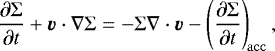
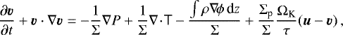
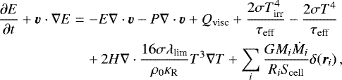
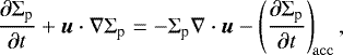
Our 2D numerical model is based on FARGO (Masset 2000) and was described in detail in Chrenko et al. (2017)1. Nevertheless, in order to present a self-contained paper, we recall the system of radiation–hydrodynamic equations (i.e. the continuity, Navier–Stokes, energy, continuity of pebbles, momentum of pebbles, equation of state, and gravity on protoplanets) and our notation here:
 (1)
(1)
 (2)
(2)
 (3)
(3)
 (4)
(4)
 (5)
(5)
 (6)
(6)
 (7)
(7)
where Σ denotes the gas surface density, v gas velocity,  gas accretion term, P vertically integrated pressure, T viscous stress tensor, ρ gas volumetric density, ϕ gravitational potential of the Sun and protoplanets, with a cubic smoothing due to a finite cell size (Klahr & Kley 2006), z vertical coordinate, Σp pebble surface density, u pebble velocity,
  pebble accretion term for both Bondi and Hill regimes (detailed in Chrenko et al. 2017), ΩK the Keplerian angular velocity, τ the Stokes number of pebbles, always assuming the Epstein drag regime, E gas internal energy, Qvisc viscous heating term (Mihalas & Weibel Mihalas 1984), σ the Stefan–Boltzmann constant, Tirr irradiation temperature (Chiang & Goldreich 1997), τeff effective optical depth (Hubený 1990), T gas temperature, H vertical (pressure) scale height, λlim flux limiter (Kley 1989), ρ0 midplane density, κR the Rosseland opacity (the Planck opacity κP hidden in τeff is assumed the same), G gravitational constant, Mi protoplanet mass, Ri protoplanet radius, Scell cell area in which it is located, μ mean molecular weight, γ adiabatic index,
  gravitational acceleration of the body i, where a smoothing is applied again for thethird term, and fz vertical damping prescription (Tanaka & Ward 2004).
More specifically, we use the following smoothing of the potential:
![\begin{equation*} {\mathrm{\phi}}_i(d) = \begin{cases} -\frac{GM_i}{d}, & \mbox{for } d > r_{\textrm{sm}}\,, \\ -\frac{GM_i}{d}\left[\left(\frac{d}{r_{\textrm{sm}}}\right)^4 - 2\left(\frac{d}{r_{\textrm{sm}}}\right)^3 + 2\frac{d}{r_{\textrm{sm}}}\right], & \mbox{for } d \le r_{\textrm{sm}}\,, \end{cases} \end{equation*}](/articles/aa/full_html/2018/12/aa33855-18/aa33855-18-eq11.png) (8)
(8)
with the smoothing length rsm = 0.5RH, where RH denotes the Hill radius of the respective protoplanet. We still integrate in the vertical direction over the density profile,
 (9)
(9)
to avoid a smoothing over H (Müller et al. 2012).
We performed a few modifications of the code, namely we improved the successive over-relaxation (SOR) solver for the radiative step, so that iterations stop when the system of equations is fulfilled at the machine precision. We also included the gas accretion term using the Kley (1999) prescription with facc parameter, even though it is switched off in most simulations. Bell & Lin (1994) local-thermodynamical-equilibrium (LTE) opacities were implemented more carefully without even minor jumps at the transitions.
The nominal simulation presented in Chrenko et al. (2017), hereinafter called CaseIII_nominal, had the following parameters: the gas surface density Σ0 = 750 g cm−2 at 1 au, slope r−0.5, the aspect ratio h = H∕r and flaring are given by radiation processes during the relaxation phase (one can start with an arbitrary value, h = 0.02 or 0.10, and the relaxation will converge to the same disc structure); adiabatic index γ = 1.4, molecular weight μ = 2.4 g mol−1, vertical opacity drop cκ = 0.6, effective temperature T⋆ = 4370 K, stellar radius R⋆ = 1.5 R⊙, disc albedo A = 0.5, softening parameter 0.5RH, the entire Hill sphere is considered when calculating disc ↔ planet interactions, the inner boundary is rmin = 2.8 au, outer boundary rmax = 14 au, a damping boundary condition (BC; e.g. Kley & Dirksen 2006) is used to prevent spurious reflections, and applied up to 1.2rmin and from 0.9rmax on; quantities are damped towards their initial values, only during the relaxation phase the damping is towards zero radial velocity; the vertical damping parameter is 0.3, pebble flux Ṁp = 2 × 10⁻⁴ M⊕ yr−1, turbulent stirring parameter αp = 10−4, the Schmidt number S c = 1, pebble coagulation efficiency ϵp = 0.5, pebble bulk density ρp = 1 g cm−3, embryo density ρem = 3 g cm−3 (constant), embryo mass Mem = 3.0 M⊕, and their number Nem = 4.
For simplicity, we used a constant kinematic viscosity ν = 5.0 × 1014 cm2 s−1 ≐ 10−5 [c.u.], but we do not expect a drastic change when we use an α-viscosity, with ν = αcsH, where cs denotes the (local) sound speed and H the scale height (Shakura & Sunyaev 1973). The viscously heated region is actually from 3 to 7 au in our nominal model, the rest is irradiated. We also do not expect (prescribe) any jumps in viscosity due to the magneto-rotational instability (MRI) and dead regions, as our disc is cold throughout.
There are several limitations to our model that we shall keep in mind. We do not account for the Stokes drag (i.e. pebble sizes Dp larger than the mean-free path ℓ), a reduction factor of the accretion rate needed for τ ≫ 1 (Ormel & Klahr 2010; Ida et al. 2016), or the gravity of pebbles (as emphasised by Benítez-Llambay & Pessah 2018). Nevertheless, our gas and pebble discs should be well within the respective limits. We find our typical pebble-to-gas ratio to be approximately 0.001, and if we assume for the moment that the results of Benítez-Llambay & Pessah (2018) are applicable even in our more complicated case (i.e. non-fixed planets, eccentric orbits, with pebble accretion, back-reaction), the ratio of torques should be Γp ∕Γg ≐ 0.05. The pebble torque can thus be safely ignored for our disc conditions.
The discretisation in space we normally use is 1024 × 1536 cells in the radial and azimuthal directions. Appendix A presents an additional convergence test. The discretisation in time is controlled by the Courant condition; the maximal time step is Δ t = 3.725 [c.u.] = 1∕20 Porb at 5.2 au. Orbital elements are output every 20 Δt, and hydrodynamical fields every 500 Δt. The nominal time span is approximately 50 kyr, but the simulations are prolonged whenever needed. The relative precision of the IAS15 integrator (Rein & Spiegel 2015) used for the planetary bodies is set to 10−9.
3 Results
Apart from the nominal case, we performed eight simulations, which are summarised in Table 1. We always changed oneparameter (or two at most) and analysed how the overall evolution changed. The dependence on the gas surface density Σ, pebble flux Ṁp, viscosity ν, embryo mass Mem, or their number Nem is a very basic question. We shall therefore describe all of them (those not so interesting included), with the most interesting implicationsdiscussed later in Sect. 4.
A very useful tool would be the construction of a complete Type-I migration map, that is a dependence of the torque Γ on the disc profiles Σ(r), T (r), the protoplanet mass Mem, and other parameters, in a similar way to Paardekooper et al. (2011) and Bitsch et al. (2013). However, in our case we have an additional parameter, namely the pebble flux Ṁp, which makes this task more difficult. It may also vary with the Stokes number τ (cf. Benítez-Llambay & Pessah 2018). At the same time, we would need an eccentricity excitation map for the derivatives ė and also for the asymptotic values easy. As we shall see in the next sections, the situation is even more complex because there are also mutual (hydrodynamical) interactions between the protoplanets.
Selected parameters of our hydrodynamical simulations.
3.1 Initial profiles
The initial radial profiles of the gas disc are shown in Fig. 1. They were obtained by a relaxation procedure, prior to the simulation itself. The initial azimuthal profiles are uniform. Several simulations actually use the same gas disc as the nominal case, namely pebbleflux_2e-5, embryos_1.5ME_8, and gasaccretion_1e-6. Another two are only extensions of the nominal case towards larger radii, namely embryos_0.1ME_120 to 16 au, and totmass_20ME from 8 to 40 au, because it turned out that the convergence zone is located in the outer disc. The profiles of the pebble disc are shown in Fig. B.1 for comparison. We assume the corresponding Stokes numbers τ are drift-limited and that initiallythe pebble flux Ṁp is independent of the radial distance.
Classically, we would expect a convergence zone somewhere between the region driven by viscous heating, and irradiation (flaring). This is no longer true when we also include the pebble accretion heating. Coincidentally, profiles for Sigma_1over3 and viscosity_1e-6 are very similar, but the disc dynamics is naturally different.
A global structure of the gas and pebble discs is shown in Fig. 2. Initially, they are very smooth but after a mere hundred orbital periods spiral arms in the gas disc are developed, the surroundings of each protoplanet and its corotation region are affected by the accretion heating, and accretion-related structures occur in the pebble disc.
3.2 Nominal case
Let us startwith a warning: for substantially non-Keplerian orbits, it is important to plot the radial distance r instead of a, q, Q (the semi-major axis, pericentre, and apocentre). For example, a spiral orbit has a perfectly smooth r(t), with no oscillations whatsoever, but its eccentricity e ≫ 0. One could be misled by non-zero e and think of close encounters between such orbits, but in fact there is always a substantial separation (cf. Fig. 3).
We briefly recall that the hot-trail effect is visible soon after the beginning of the simulation; at t ≃ 100 Porb, there are developed oscillations of r(t) (which would correspond to the eccentricity up to 0.035). The zero-torque radius in the absence of accretion heating would be located at about 7 au where the disc becomes flared by stellar irradiation. Instead, we see that planets migrate towards 9 au. Such an offset is due to the accretion heating, which adds a positive torque contribution, and also the hot-trail effect, because the Lindblad and corotation torques become modified for oscillating orbits.
No low-order mean-motion resonances (MMR) are established during migration, partly because the embryos were initially too close, so no captures are expected even if the simulation is run for longer. Resonances 3:2, 4:3, 5:4, and so on were encountered, but a resonant capture would in any case be difficult, because e > 0 (Batygin 2015). During the series of close encounters, there are about 20 exchanges when orbits radially swap, five repulsions when the distance between orbits increases, and two successful mergers, 13.8 and 4.3 M⊕, which finally settle to a co-orbital configuration (Fig. 3).
In the following, we show details of two representative events: the merger and the co-orbital formation. We discovered that three-body interactions are needed for successful mergers. One can see already from r(t) that a third embryo is “always” (two out of two cases) present in the vicinity.
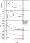 |
Fig. 1 Profiles of the gas disc after the relaxation phase, which serve as the initial conditions for our simulations. From top to bottom panels: opacity κ, the aspect ratio h = H∕r, the temperature T, and the surface density Σ. The grey boxes indicate the extent of the damping zones at the inner and outer BC. The vertical dotted lines show the snowline, and the transition between the viscous heating and the stellar irradiation regions, in the case of the nominal simulation. Some of the simulations actually use the same disc as the nominal one. For totmass_20ME simulation we had to use an outer disc, spanning from 8 to 40 au. Similarly, we used a slightly larger disc (up to 16 au) for the simulation embryos_0.1ME_120. |
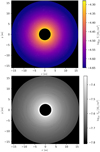 |
Fig. 2 Initial global structure of the gas and pebble discs in one of our simulations. Top panel: gas surface density Σ; bottom panel: pebble surface density Σp. In our model the discs interact mutually by means of an aerodynamic drag, and also with protoplanets by means of gravitation (in case of gas) and accretion. |
3.2.1 Detail: merger
In order to resolve a detail, the simulation has to be restarted from hydrodynamical field files prior to the time of interest. We used at least 100 times finer output (every Δt). The evolution is not always exactly the same; for example the SOR method (its relaxation factor) depends on past evolution. Nevertheless, the merger event at t≐ 2609 Porb was repeated perfectly, as shown in Figs. 4, 5, and B.2.
First, embryo 4 scatters off embryo 3 during a deep encounter, with a minimum separation being a small fraction of the Hill radius, RH ≐ 0.15 au. Second, embryo 4 encounters embryo 2 during the next orbit, so they merge. Without the prior strong perturbation, the collisionwould not occur. At the same time, there are disc torques that substantially affect the evolution (Fig. 6). Prior to the merger, they brake the outer embryo 4. It seems that the relative motion in the z-direction is not important in our situation, being a small fraction of the embryo radius, Δ z ≪ Rem ≃ 10−4 au.
We also performed a test with a purely N-body integration in order to check whether this event is caused either by a mutual gravitational interaction between the embryos or by hydrodynamics. The integration was restarted from the same time, the derivatives being the same, but without any disc torques the orbits are Keplerian most of the time, so both encounters have different geometries and a merger event does not occur at all. One can see the actual difference in Fig. 5.
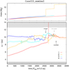 |
Fig. 3 Semi-major axis a (line), the heliocentric distance r (dots) versus time t (bottom panel), and the embryo mass Mem versus t (top panel) for the nominal simulation with initially four embryos. The time span 4000 Porb correspondsto 47.4 kyr. Although it was already presented in Chrenko et al. (2017), we show it here to provide an easy (1:1) comparison. The grey strips indicate the inner and outer damping regions used to gradually suppress spurious reflections. The black arrows indicate two interesting events we study in detail: a merger (3+4), and a co-orbital formation. The semi-major axis may exhibit a “spike” during a close encounter, but in fact r ≪ a; the body is far from the damping zone. |
3.2.2 Detail: Co-orbital
As shown in Fig. 7, the co-orbital was formed at t ≐ 3310 Porb by an encounter of the less-massive embryo 1 with the more-massive embryo 2 from behind. During the approach, embryo 1 flies through a detached or prolonged spiral arm of embryo 2. The corresponding disc torque suddenly changes from negative to positive (normalised Γ ≃ 50; Fig. 6). We stress these torques would be calculated wrongly in N-body models, which use prescriptions derived for single planets. On the departure, the former embryo enters an underdense region and is captured in the co-orbital region of the latter.
While we do not model a long-term evolution of the co-orbital pair here, we can assume its stabilisation according to Sect. 3.6. Similarly as before, without the disc torques only an orbital exchange would occur. Co-orbitals are generally common outcomes of the simulations, because the resonant captures are prevented by non-zero eccentricities.
3.3 High surface density
For a surface density three times larger than the nominal case, as in the Sigma_3times simulation, the surface-density structures of the hot-trail effect are not so pronounced, owing to the larger thermal capacity of the gas (i.e. the specific capacity multiplied by Σ). The temperature excess reaches up to 10 K, not 20 K as before. The 0-torque radius is located further out at approximately 11 au. The oscillations r(t) are relatively small, with the radial distance systematically smaller than the semi-major axis, r < a, because the interior disc mass ∫ Σ(r)2πrdr ≃ 0.03 M⊙ is no longer negligible. This is also a notable case of non-Keplerian orbits, and a “false” osculating eccentricity e > 0, which shall no longer be used. Generally, the evolution seems slower, although the time span in Fig. 8 is almost three times longer and the migration rate is comparable to the nominal case, d a∕dt ≃ 10−3 au∕Porb.
Embryos do not interact so strongly; their orbits stay next to each other for a prolonged period of time, probably because the hydrodynamical eccentricity damping is strong. Sometimes, there is a reverse inward migration of the inner embryo 1 or 2, inducing also larger oscillations of r(t). Moreover, these excursions seem to be often out of phase, and so they are not of a resonant, but rather of a hydrodynamical origin.
Interestingly, there are more than 10 attempts by embryos 3 or 4 to enter the co-orbital region of each other. More specifically, there are in total 17 repulsions, 20 exchanges, two temporary co-orbitals, and eventually one merger, again soon after an encounter with another embryo. The last part is already affected by interactions with the disc edge and the damping zone, which kills the outer spiral arm.
Detail: Repulsion
A detail of a repulsion event is shown in Fig. 9, namely the first one at t ≐ 1945 Porb. Embryos 3 and 4 approach each other in the apocentre and pericentre, respectively, and their spiral arms are thus aligned. At the minimum distance of just 2RHill, there is an overdensity between them.
The disc torque during this event is shown in Fig. 6, in comparison with other types of events. It seems there are alternating torques for the inner and outer embryos, which contribute to the repulsion of the two. The next encounter isconsequently more distant. An alternative Fig. B.3 expressed in terms of the semi-major axis a(t) also shows that the closest encounter itself is driven by the interaction between the embryos, and the disc torque acts as a perturbation. Nevertheless, the regular and repeated nature of these repulsion events confirms that the torque actually determines the encounter geometry.
3.4 Low surface density
Generally, one would expect two limits to exist: for Σ →∞ the thermalcapacity is so large, no hot-trial effect can develop; for Σ → 0 there is no hot trail because there is no gas. In the simulation Sigma_1over3, we use the surface density corresponding to 1/3 of the nominal (Fig. 10). It turns out that the hot trail is even larger compared to the nominal case. This is a result of smaller thermal capacity, and also lower disc temperature, which allows for a larger temperature excess. Its development takes longer (more than 200 Porb) and the trajectories seem to be more regular.
Overall the migration rate is comparable, although later the motion often exhibits “jumps”, because the hydrodynamical damping is weaker. There are 28 exchanges, nine repulsions (at least), no co-orbitals, and no mergers in the course of the evolution. Given this statistics, it is compatible with the nominal case (after a normalisation to the same time span 4000 Porb); co-orbitals and mergers are a matter of small-number statistics, however. One would need a sample of 102 simulations to determine which of the simulations would produce more of these relevant outcomes.
 |
Fig. 4 Gas surface density Σ in the (x, y) plane for a very short segment (t = 2605 to 2610 Porb at 5.2 au) of the CaseIII_nominal simulation, showing approximately one long-period orbit during which a three-body interaction occurs, and results in a merger event. The y-coordinates are differentfor individual panels, but the overall range is always 4 au. The Sun is located at (0,0). The positions of the embryos areindicated by their Hill spheres (circles) and heliocentric distances (labels, in au units). The motion is in an anti-clockwise direction. |
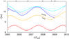 |
Fig. 5 Heliocentric distance r versus time t for all four embryos in the simulation shown in Fig. 4. The black triangles correspond to the time of individual snapshots. There is an output from the full hydrodynamic simulation (lines), and an N-body simulation with no discs and no torques (points) for comparison. The latter was restarted from the very same initial conditions, at t = 2605 Porb. One can see the merger event at t ≐ 2609 Porb. In the case of the N-body simulation, the evolution is different, because without the disc torques the trajectories are mostly Keplerian, the encounter between embryos 3 and 4 just one orbit prior to the merger (2+4) has a different geometry, so the merger actually does not occur. |
3.5 Low pebble flux
Yet another limit is clear: for Ṁp → 0 the heating is zero, as is the hot-trail effect. The opposite case Ṁp →∞ is unclear (and unrealistic). For the simulation pebbleflux_2e-5, we chose the pebble flux ten times lower, corresponding to the embryo growth rate of only 0.25 M⊕ per 4000 Porb. This may be actually more realistic in later phases (Lambrechts & Johansen 2014); the nominal case was on the high side, so we consider this simulation to be potentially very important.
As expected, hot-trail oscillations take longer to develop (1000 Porb), and they are about three times smaller afterwards (Fig. 11). The evolution is consequently more smooth, with no “jumps”, until the embryos migrate to the convergence zone at about 11 au. This value seems somewhat surprising, because the heating is substantially lower, and the 0-torque radius should be rather smaller than the nominal one, r < 9 au. However, an equilibrium (of Lindblad, corotation, and heating torques) is perturbed here by the oscillations, and can be therefore shifted elsewhere. For example, a small outward excursion takes the embryo closer to the trailing spiral arm, without actually crossing it, while a large excursion can reverse the Lindblad torque, which is somewhat counterintuitive.
The situation later dramatically changes, as there is one quick merger, no co-orbitals, two exchanges, two big repulsions (plus many small ones), because the torque acting on the 6 M⊕ merger is so strong, it drives it outwards in a runaway mode (Pierens & Raymond 2016). Obviously, this is the explanation for Planet IX. Taken more seriously, it turned out to be a rule for more massive embryos (see Sect. 3.8). This also leads to a clearing of the outer disc beyond 11 au. The two remaining embryos 1 and 3 still migrate outwards, their proper 0-torque radius being further out. From the point of statistics, this simulation is not necessarily a representative one, and the early merger can be easily avoided with a minor shift in the initial conditions.
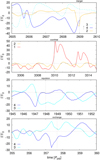 |
Fig. 6 Normalised total disc torque Γ∕Γ0 versus time t, where |
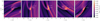 |
Fig. 7 Same as Fig. 4, but for a co-orbital formation during the interval t = 3305 to 3315 Porb. The less-massive embryo approaches the more-massive one from behind, flying through its inner (detached) spiral arm, entering the co-orbital region, and flying away into a low density region. |
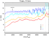 |
Fig. 8 Semi-major axis a, and the heliocentric distance r versus time t for the simulation Sigma_3times. The convergence radius is shifted further out to 11 au. Merging seems more difficult in this case as there are many “repulsions”, especially between embryos 3 and 4. The black arrow indicates the repulsion event we study in detail. The semi-major axis is systematically offset from the radial distance, a > r, because the orbits are substantially non-Keplerian. After approximately t ≐ 10 000 Porb some unwanted interaction with the disc edge occurs and the evolution is no longer reliable. The masses reach 5–7 M⊕ prior to this. |
3.6 Low viscosity
As discussed in Sect. 1, the disc – or its dead zone with a negligible ionisation and no MRI turbulence – could have been also (almost) inviscid. For this purpose, we performed a simulation with ten times lower viscosity (code-named viscosity_1e-6). The structures in the gas disc shown in Fig. 12 are more pronounced; the viscous spreading is diminished, thus any density perturbation arising from protoplanets persists for longer.
The evolution itself (Fig. 13) indicates the same hot-trail oscillations, but a faster migration towards the 0-torque radius (Paardekooper et al. 2011). Embryos pushed by larger torques then interact more violently and this results in 18 exchanges, 19 repulsions, two mergers – created by three-body interactions – and five co-orbitals, in total. Out of these, four are only temporary and experience another three-body interactions, during which they exchange their members (around t ≐ 2000 Porb). The last one, formed by two 8 M⊕ embryos, is stable, and is further stabilised.
This stabilisation is facilitated by a pebble isolation that develops beyond the co-orbital pair (Fig. 12, bottom panel; seen as a stalled accretion Ṁem ≐ 0 in Fig. 13, top panel). It also implicitly drives the migration inwards; it switches off accretion heating by isolating the co-orbital from further solid material. The pair is massive enough to create a surface density contrast of about 2 between the interior and exterior part of the gas disc, or 2.5 if we take the middle of the gap. Nevertheless, both are still optically thick; it is not yet a gap opening. Unless there is a substantial filtering of dust (Rosotti et al. 2016), or an extensive shadow hiding the outer part, or very long wavelengths (λ ≫ adust) are used, it would be difficult to observe.
Detail: Exchange
A detail of the first exchange is shown in Fig. 14. Embryo 3 at the apocentre encounters embryo 4 at the pericentre. An overdense region is formed between them as the outer and inner spiral arms overlap. During the closest approach at a distance of 1.2 RH, the gas distribution is uneven. As the embryos become more distant, an extended underdense region is formed between. Disc torques contribute to the exchange, being mostly negative on the outer embryo and positive on the inner one (Fig. 6). Apart from these major perturbations, there are many more minor density waves created by other (inner) embryos.
 |
Fig. 9 Same as Fig. 4 for a repulsion event in the Sigma_3times simulation, which occurred between t = 1945 to 1952 Porb. The embryos approach each other in the apocentre and the pericentre, respectively, with spiral arms “aligned”. There is an overdensity between the Hill spheres during the closest approach, and yet another spiral arm originating from the inner embryo 2 after the close approach. |
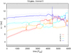 |
Fig. 10 Same as Fig. 3 for the simulation with Σ0 three times smaller than the nominal one. The oscillations r(t) induced by the hot-trail effect are larger compared to the previous case, and also seem more stable. There are numerous encounters in the evolution, but no mergers yet. The final masses reach 5–6 M⊕. |
3.7 Gas accretion
As a test, we also performed a simulation with the gas accretion and the corresponding heating switched on, but the efficiency parameter was very small, facc = 10−6, as we started with 3 M⊕ bodies. Specifically, the gas accretion rate is given by the integral over the exponential density profile (Kley 1999),
![\begin{eqnarray*} \left(\frac{\partial{\mathrm\Sigma}}{\partial t}\right)_{\textrm{acc}} &=& \sum_i \frac{1}{3}f_{\textrm{acc}} \int\!\!\!\int {\cal H}(|\vec r_{\perp i}-\vec r_{\textrm{cell}}|-0.75 R_{\textrm{H}i}) \nonumber\\ && \times\, \frac{{\mathrm\Sigma}}{\sqrt{2{\mathrm{\pi}}}H} \int_{z_i-{\mathrm{\Delta}} z}^{z_i+{\mathrm{\Delta}} z}\! \exp\left[-\left(\frac{z}{\sqrt{2}H}\right)^2\right] \textrm{d} z\,\textrm{d}{\mathrm{\theta}}\textrm{d} r\,, \end{eqnarray*}](/articles/aa/full_html/2018/12/aa33855-18/aa33855-18-eq13.png) (10)
(10)
plus the same term with numerical factors  and 0.45, where
  denotes the Heaviside step function, r⊥ the planet position in (x, y) plane,
 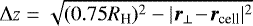 , and H the vertical scale height.
The total amount of gas thus reaches at most 0.035 M⊙. We may regard this simulation more as another realisation of the nominal one. Indeed, according to Fig. 15, the hot-trail oscillations are practically the same, as are the migration rates. The difference stems from the chaotic nature of the system. A comparison of the first 4000 Porb shows a similar frequency of the common events, albeit there are no co-orbitals or mergers yet, which are simply not frequent enough to occur in every simulation. We did not continue the simulation because of the interactions with the outer damping zone.
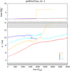 |
Fig. 11 Same as Fig. 3 for the pebble flux Ṁp 10 times smaller than the nominal case. The hot-trail effect (es) are then smaller than in the nominal case. After a merger at t ≐ 2250 Porb, the resulting6 M⊕ embryo quickly migrates outwards and is lost at the outer BC. |
3.8 Four 5 M⊕ embryos
With initial masses 5 M⊕, all embryos quickly drifted outwards. The 0-torque is clearly much more distant, and our setup requires an outer disc spanning from 8 to 40 au (i.e. totmass_20ME). In other words, this may be relevant for the formation of ice giants. The spacing of embryos is 16 mutual Hill radii, similar to before. We also deliberately decreased the pebble flux to Ṁp = 10−5 M⊕ yr−1, because larger embryo masses are usually attained later. A convergence to the new 0-torque radius at about 20 au is relatively fast, especially when longer orbital periods are taken into account (Fig. 16).
The evolution is similarly complex as in the inner disc, with 20 exchanges, five repulsions (not counting the small ones), two mergers, and two co-orbitals, with the last one (at t ≐ 4000 Porb) stabilised; this time it is not due to the pebble isolation, but rather pebble filtering due to embryo 1, which has became the outer massive merger in the course of evolution.
A very interesting behaviour then starts: embryo 1 is pushed outwards by a dynamical torque created by an underdense tadpole-like region (Pierens 2015). Later at t ≐ 4900 Porb, when embryo 1 reaches its new convergence radius rc, it slightly overshoots, is pushed backwards, and the tadpole region is refilled by a material originating from the inner spiral arm. With no underdensity anymore, embryo 1 is pushed inwards, until it encounters the co-orbital. This behaviour is systematically repeated four times, with a disruption of the co-orbital in the meantime, and a second merger after all.
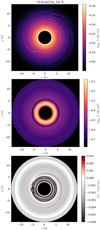 |
Fig. 12 Surface density Σ for the simulation with 10 times smaller viscosity ν; the situationshort after the beginning at t = 100 Porb (top panel), and the final state at t = 8000 Porb (middle panel). The structures are initially more pronounced compared to the nominal case, because perturbations of the low-viscosity gas spread more slowly. The outcome is a massive co-orbital that migrates towards the inner boundary. The density contrast between Σ interior and exterior to the co-orbital is about 2; the disc is optically thick in both cases. The corresponding azimuthal velocity uθ of pebbles (bottom) is compared to the Keplerian velocity vkepl. Just outside the co-orbital pair, the dimension-less ratio (uθ − vkepl)∕vkepl is positive (uθ super-Keplerian) and a pebble isolation develops. |
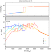 |
Fig. 13 Same as Fig. 3 for the simulation with ten times smaller viscosity ν. The oscillations r(t) are initially similar to the nominal case, but there is a faster migration towardsthe convergence radius. After many “trials”, there are two mergers (8 M⊕), which later form the co-orbital pair. The black arrow indicates the repulsion event we study in detail. |
3.9 Eight1.5 M⊕ embryos
For eight embryos with 1.5 M⊕ each, we can see a clear convergence to the 0-torque radius at approximately 9 au (as in the nominal case). The oscillations due to the hot trailare apparently small for the innermost embryos, but they become larger as they migrate outwards. At the given radial distance, the amplitudes are the same (Fig. 17).
The migration is slower compared to the nominal case, nevertheless the initial spacing is more compact (10 mutual Hill radii), and interactions start at about the same time. They are of all kinds, both two-body and three-body, but we will not count them explicitly, as the number of objects is two times larger. Generally, there are more opportunities to merge, ending up in five mergers, the most massive having up to 25 M⊕. From this standpoint, the simulation can be termed as successful, creating a giant-planet core with more than a critical mass. Our current model is not reliable for this large mass though, as we used no Hill cut, zero gas accretion efficiency factor facc, and there are problems in describing the pebble isolation in 2D (Bitsch et al. 2018). A sixth merger occurred after a series of unwanted interactions with the outer damping zone, and this makes further evolution also unreliable.
In this simulation (and also in viscosity_1e-6), the embryos gain non-negligible temporary inclinations of the order of 10−4 rad, despite Tanaka & Ward (2004) damping. The vertical distances are then orders of magnitude larger than protoplanet diameters, which decreases collisional probabilities. On the other hand, a gravitational focussing (with vesc ≐ 7 km s−1) – which is accounted for in our model – helps to counteract it.
 |
Fig. 14 Same as Fig. 4 for an exchange event in the viscosity_1e-6 simulation. Embryos 3 and 4 approach insuch a way; the inner flies behind the outer and a shared underdense region is formed that connects the embryos during their retreat. |
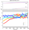 |
Fig. 15 Semi-major axis a (line), and the heliocentric distance r (dots) versustime t (bottom panel), and the embryo mass Mem versus t (top panel) for the simulation including the gas accretion, with the efficiency factor facc = 10−6. We distinguish the solid (solid) and gaseous (dashed) component of Mem. We used a finer sampling of the orbital elements. Both the migration rates and the eccentricities seem the same as in the nominal case, because the gas accretion contributes only very little to the mass and heating. However, no merging occurred in the course of this simulation. After t ≐ 6400 Porb, there is an interaction with the disc edge and the evolution is no longer reliable. |
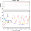 |
Fig. 16 Same as Fig. 3 for the simulation with 5M⊕ embryos. We model an outer disc here, because the convergence radius turned out to be far (21 au). After numerous exchanges, temporary co-orbitals, and one merger, a relatively stable co-orbital is formed at t ≐ 4000 Porb. Embryo 1 isthen pushed outwards by a dynamical torque created by an underdense tadpole-like region (Pierens 2015). At t ≐ 4900 Porb the tadpole region is refilled by a material originating from the inner spiral arm, and embryo 1 is pushed inwards, until it encounters the co-orbital. This behaviour is systematically repeated, and results in a disruption of the co-orbital, and a merger. |
3.10 Many low-mass embryos
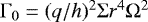
Finally, we simulated a system composed of 120 embryos with 0.1 M⊕ each (i.e. embryos_0.1ME_120); the total mass remains the same as the nominal. We chose a tight spacing of two mutual Hill radii:
 (11)
(11)
with a the semi-major axis and q the planet-to-star mass ratio, to fit all bodies in a disc spanning from 2.8 to 16 au. The initial state was already shown in Fig. 2. A convergence test for a single embryo is presented in Appendix A. Our current resolution is still low, three cells per Hill sphere. The test shows that d a∕dt is then overestimated by a factor of 3, and r(t) oscillations (or eccentricity e) have the same amplitude. We consider this as an acceptable approximation that may somewhat enhance the efficiency of merging (due to larger da∕dt). Having correct eccentricities seems more important to prevent spurious resonant captures. It is in any case a very slow computation, with 120 disc ↔ planet interactions; because of this it was run on the NASA Pleiades supercomputer, with 103 reserved CPU cores, and a combined MPI/OpenMP parallelisation. To better resolve the Hill sphere, one would have to increase the number of cells in both radial and tangential directions, fulfil the Courant condition in these smaller cells, and compute all the interactions, so it scales almost as N3Nem.
The most important result is visible already at the beginning – there is no smooth Type-I migration, because there are no regular patterns (see Fig. 18). The weak spiral arms overlap and also affect neighbouring corotation regions. These stochastic torques are very different from the classical, regular, single-planet torques. Although Type-I migration in its simplest form may be considered linear, it is no longer true because our system of equations (Eqs. (1)–(7)) includes several non-linear terms (T 3, T 4, Qvisc). Mutual gravitational interactions of the embryos also partly contribute to the stochastic nature of the system, especially given the initial spacing (2 RHH).
The evolution of the whole system is surprisingly slow (Fig. 19). The oscillations induced by the hot-trail effect (e≐ 0.02) serve as an initial “kick”, which leads to numerous close encounters. At the same time, inclinations i are also excited, being virialised with the eccentricities e. The average values are different however, e ≃ 0.02, i ≃0.01 rad, because Tanaka & Ward (2004) damping acts on inclinations. This is a new situation; in all previous simulations inclinations remained low (less than 10−3 even during close encounters). Given the increase of e, we expectedthat there will be many mergers early in the simulation, but this is suppressed by the increase of i. There are only 11 of them that occur during the first few 100 Porb, creating a group of 0.2ME embryos, located both in the inner and outer parts of the disc. It might be an artifact of our initial conditions, but it does not “compromise” our results in any way, because having a range of masses initially seems even more realistic.
Further growth is facilitated mostly by pebble accretion. Only a handful of additional mergers occur (see Fig. 19, top panel). We identified five processes that contribute to a runaway growth: (i) the initial mergers (0.2 M⊕), other embryos have a mass “handicap”; (ii) in the Hill regime of pebble accretion, the cross section is proportional to the embryo mass,  , and the relative velocity too,
  , which results in an exponential Mem(t) evolution; (iii) late mergers of inner embryos occur, which subsequently drift outwards; (iv) pebble filtering by outer (already massive) embryos; (v) a separation between low- and high-mass embryos, with the former having larger mean inclinations than their pebble feeding zone (Fig. 20). The peak masses are almost 3 M⊕ for the group of early mergers, while only 0.6 M⊕ for the group of original embryos.
The pebble filtering is closely related to a “gap” that develops in the pebble disc (Fig. 21, bottom panel). Pebbles drifting inwards experience a strong filtering, and Σp decreases as r → 0. The apparent increase of Σp at r ≃ 6 au is only due to a flux conservation towards the centre. The “winning” embryo is consequently located in the outer part of the disc, because it experiences almost no filtering.
The separation of inclinations, or in other words a viscously stirred pebble accretion, was studied by Levison et al. (2015), using a Lagrangian approach. Indeed, in our case τ ≃ 0.05, αp = 10−4,  , h = H∕r ≃ 0.04, hp = tan Ip ≃ 0.0018, that is, a similar value to that presented in their work.
Finally, the most massive embryos exhibit a systematic drift towards a 0-torque radius at approximately 11 au, although it is somewhat hidden in Fig. 19. Low-mass ones randomly walk (with a  characteristic). As soon as they reach the interaction zone of high-mass ones, they start to randomly “run”, because the zone is very chaotic.
Luckily, the final state of the system is quite similar to the initial conditions of the simulation CaseIII_nominal. There are four embryos with masses between 1.5 and 3 M⊕. They are already located close to the 0-torque radius and they already interact with each other. We do not think this is a mere coincidence, but rather an indication that our model can self-consistently describe both phases of evolution in one elegant step.
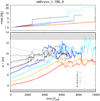 |
Fig. 17 Same as Fig. 3 for the simulation with eight 1.5M⊕ embryos. The evolution seems qualitatively similar to the nominal case, with six merger events. Most if not all mergers occur when three-body interactions take place. After t ≐ 8750 Porb, an interaction of the outer embryo with the disc edge occurs and the evolution is no longer reliable. |
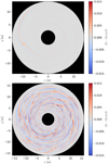 |
Fig. 18 Surface density Σ(r, θ) of the gas disc with the azimuthally averaged profile Σ(r) subtractedto clearly see the respective spiral arms, the corotation region, and other perturbations in the surroundings of the Hill sphere. The system was evolved for 100 orbital periods Porb (at 5.2 au) so that the hot-trail effect can develop and increase the eccentricity. The situation is very different for a single 0.1 M⊕ embryo (top panel), with a very regular spiral, and for 120 embryos with the same masses (bottom panel), with spiral arms overlapping each other and creating an irregular overall pattern. The situation corresponds to Fig. 2, but it is much easier to see the perturbations when Σ − Σ (r) quantity is used. The resolution 3072 × 4096 was used for the former short-term simulation, and 2048 × 3072 for the latter. The Hill spheres are shown as small black circles. |
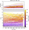 |
Fig. 19 Semi-major axis a versus time t (bottom panel), and the embryo mass Mem versus t (top panel) for the simulation with 120 low-mass 0.1M⊕ embryos. Colours correspond to the embryo number to distinguish the individual orbits. The final state is depicted as a series of filled circles, with sizes proportional to the masses. The evolution is never regular but rather chaotic, partly due to direct N-body gravitational interactions among the embryos, but more importantly due to overlapping spiral arms(see also Fig. 18). Initially, there are only several mergers that create a handful of 0.2M⊕ embryos. These grow preferentially by the pebble accretion; there are a few additional mergers. |
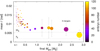 |
Fig. 20 Mean inclination Ī (rad) versus the final embryo mass Mem. The symbol sizes correspond also to Mem and their colours to the embryo number, or its initial position. The horizontal dotted lines indicate multiples of the pebble scale height, hp = Hp∕r. The smaller vertical distance of the massive embryos from the pebble disc contributes to a runaway growth. All embryos are already in the Hill regime, and their effective accretion radius ranges from Reff ∕r = 0.003 to 0.012. |
4 Conclusions
The simulations of the Type-I migration presented in this study confirm that outcomes sensitively depend on the disc parameters, as well as the initial conditions and masses of protoplanets. We reported at least severalinteresting results: (i) three-body encounters are needed for successful mergers; (ii) in high-Σ discs (several times minimum-mass solar nebula; MMSN) “repulsion” events are frequent; (iii) a massive co-orbital pair may develop a pebble isolation that prevents further accretion; (iv) a stabilisation and inward migration of the co-orbital then occurs; (v) a dynamical tadpole torque can arise in the outer disc (as in Pierens 2015); (vi) this leads to outward ↔ inward migration cycles; (vii) the respective fast-migrating embryo may disrupt an inner co-orbital pair, solving the problem of too many co-orbitals that are not observed (Vokrouhlický & Nesvorný 2014); (viii) disc torques for many low-mass embryos are stochastic, due to overlapping spiral arms, and the torques computed for single planets (as in Paardekooper et al. 2011) are no longer valid in this regime. This may have very important implications for N-body models of planetary migration.
In the gas-giant zone, our simulations show a robust runaway growth with several contributing processes, in particular the above-mentioned merging of embryos, the Hill regime of pebble accretion, which is proportional to Mem, pebble filtering by outer embryos, and lower inclinations of massive embryos (being often within the pebble disc scale height), further supporting the results of Levison et al. (2015).
In the ice-giant zone (at 20 au), there is a surprising convergence zone for more massive (5 M⊕) embryos, or mergers that may originate from the gas-giant zone. This could possibly support scenarios in which Neptune forms first, Uranus second, and so on – in an opposite way to that described in Izidoro et al. (2015).
We may be actually seeing different phases of a “Grand Scenario”, outlined, for example, by the following sequence of simulations: embryos_0.1ME_120 → embryos_1.5ME_8 → pebbleflux_2e-5 → totmass_20ME. Of course, it would be better to have everything in one simulation (and a big disc, spanning at least from the water snowline to the outer edge, if there was any).
The time span of our longest simulations is about 150 kyr. If the total available mass of solids is of the order of 130 M⊕ (as in Levison et al. 2015), and the pebble flux reaches up to 2 × 10⁻⁴ M⊕ yr−1, its duration could be as long as 650 kyr. It is thus still possible to prolong our simulations using the current setup.
Ideally, one would like to continue until the gap opening in the gas disc, which would however require a better treatment of the pebble isolation (Bitsch et al. 2018); a suitable parametrisation of the gas accretion, derived in full 3D, not in 2D (Crida & Bitsch 2017); or even until photoevaporation, probably including a model for the disc atmosphere (Owen et al. 2011), and inevitably also a planetesimal (debris) disc, which stabilises the emerging compact planetary systems.
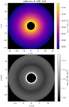 |
Fig. 21 Gas surface density Σ (top panel) and pebble surface density Σp (bottom panel) close to the end of the simulation embryos_0.1ME_120, at t = 11 200 Porb. It is a continuation from Fig. 2. There are relatively massive embryos present in the disc, reaching up to 3 M⊕ (cf. the spiral arms). They concentrate in the outer part of the disc. In the pebble disc, one can see a darker region (low Σp) in the middle, which arises from a substantial pebble filtering by the outer embryos. The resolution 1024 × 1536 was used forthis long-term simulation. |
Acknowledgments
The work of MB and OC has been supported by the Grant Agency of the Czech Republic (grant No. 18-06083S). The work of OC has been supported by Charles University (research programme No. UNCE/SCI/023; project GA UK No. 128216; project SVV-260441). DN’s work was supported by the NASA XPR programme. Access to computing and storage facilities owned by parties and projects contributing to the National Grid Infrastructure MetaCentrum, provided under the programme “Projects of Large Research, Development, and Innovations Infrastructures” (CESNET LM2015042), is greatly appreciated. We also thank A. Morbidelli and E. Lega for fruitful discussions on the subject, the anonymous referee, and the editor (T. Guillot) for constructive criticism.
Appendix A A convergence test for 0.1 M⊕ embryos
We simulated a solitary embryo with the mass Mem = 0.1 M⊕, embedded in the gas and pebble discs. Practically, the setup corresponds to the simulation embryos_0.1_120 from the main text. We used the following resolutions (in r, θ): 512× 768 (very low), 1024 × 1536 (low), 2048 × 3072 (moderate), and 3072 × 4096 (high). Per Hill sphere, these correspond to 1.5, three, five, and eight cells in the radial direction. The outcome is summarised in Fig. A.1. The semi-major axis exhibits different migration rates; for very low and low resolution they are three to four times as large as for the moderate or high resolutions. This is due to a poor resolution of the Hill sphere, and the corotation region.
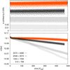 |
Fig. A.1 Temporal evolution of the semi-major axis (bottom panel) and the eccentricity (top panel) of a single low-mass 0.1 M⊕ embryo embedded in the gas and pebble discs, for four different discretisations in space, namely 512 × 768 cells in r and θ (i.e. a very low resolution), 1024 × 1536 (low), 2048 × 3072 (moderate), and 3072 × 4096 (high). Theamplitudes eccentricity oscillations are approximately the same for all cases, even though the torques have much larger amplitudes for very low and low resolutions. To obtain a correct value for the migration rate d a∕d t, one would need the moderate resolution at least. The rate da∕dt is about three times as large for the low resolution. |
On the other hand, the eccentricity oscillations have rather similar amplitudes over the given time span (albeit the temporal evolution is somewhat undersampled). If we look at the torques in low-resolution simulations, they vary with much larger amplitudes, but on average the eccentricities seem to be sufficiently similar. The moderate and high resolutions may exhibit a long-term trend towards a larger asymptotic value.
Appendix B Supporting figures
Figures B.1 to B.3 show the simulations discussed in the main text in an alternative way.
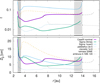 |
Fig. B.1 Pebble sizes Dp (top panel), the corresponding Stokes numbers τ (bottom panel), and their dependence on the radial distance r in individualsimulations. The value of Dp changes in such a way as to keep the pebble flux Ṁp initially constant. On the other hand, the value of τ is inversely proportional to the coupling between the gas and pebbles. Both quantities are increased in the damping zones (grey strips), but this does not affect our simulation in any way. |
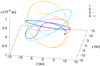 |
Fig. B.2 Same as Fig. 5 shown in 3D. It can be seen how the encounter proceeds in the vertical direction. The scale of the z coordinate isvery small (10−6 au). The subsequent merger event is denoted by “M”. |
Nevertheless, we decided to use 1024 × 1536 at this stage of research, because the computations would be otherwise prohibitively expensive in terms of the CPU time. We also thought the evolution may be quick enough that the high resolution actually would not be needed for the whole simulation time, if some mergers occur soon for which this resolution is sufficient.
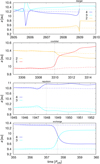 |
Fig. B.3 Semi-major axis a(t) evolution corresponding to the torques Γ in Fig. 6. The actual orbital evolution (solid lines) of the embryos is shown together with a fictitious trajectory (dashed) obtained from the disc torques only, as an integral of the first Gauss equation, d a∕d t = 2Γ∕(rn), where r denotes the radial distance and n the mean motion. |
Appendix C Context and subsequent evolution
In order to provide a broader context for our work and the expected timescales of a subsequent evolution, we append a few remarks. The protoplanets we focus on in this paper (with initial masses ranging from 0.1 to 5 M⊕) do not open a gap in the disc, and this phase is generally called a (fast) Type-I migration. Its typical timescale (at the distance of Jupiter 5.2 au) is of the order of 10 kyr, after which the radial distance changes substantially, protoplanets start to interact, and so on. Only if the planetary core becomes critically massive (≃ 20 M⊕) does it accrete and repel gas from the corotation region – possibly in only 102 orbital periods – and the respective torques are zeroed (Lin & Papaloizou 1986; Crida & Morbidelli 2007; Crida & Bitsch 2017). The remaining distant spiral arms couple the planet to the disc, which is driven by the viscosity ν, and thus a (slow) Type-II migration should occur, with the timescale given by  , that is, on the order of 100 kyr
While we do not study the viscous properties of the disc in any detail, we should note the (eddy) viscosity ν is actually used to describe underlying (unresolved) turbulent flows, which effectively exchange the angular momentum between differentially rotating layers. This turbulence can be driven by the vertical shearing instability (a.k.a. Kelvin–Helmholtz in z direction; Nelson et al. 2013), subcritical baroclinic instability (essentially, Rayleigh–Taylor with heat diffusion; Klahr & Bodenheimer 2003), magneto-rotational instability (Balbus & Hawley 1991; Turner et al. 2014), although it can be suppressed in dead zones where the ionisation is too low, or spiral wave instability (resonant coupling between spiral arms induced by an embedded planet and inertial-gravity waves; Bae et al. 2016). Theoretically, it is also possible that the accretion inflow is driven by a stellar wind (Günther 2013; Turner et al. 2014), if it was not weak, X-wind at the disc edge (Shu et al. 1994), or by magneto-centrifugal wind and loading of ions (Anderson et al. 2005; Suzuki et al. 2016), which can all affect the disc surface and carry some part of the angular momentum away.
From the observational point of view, a full disc should become pre-transitional (as defined by Espaillat et al. 2014) in the course of the outlined evolution. Transitional or even evolved discs correspond to much later phases. In the framework of young stellar object (YSO) classification, based on 2.2 to 20 μm spectral slope of λFλ, it corresponds to Class II objects with moderately negative slope. The above-mentioned gap opening should eliminate a part of the disc with moderate temperatures and result in a pronounced decrease of spectral-energy distribution around λ ≃ 10 μm.
At the same time, the central star (Sun) irradiating the disc is a pre-main sequence object of T Tauri type, for which we assume parameters M⋆ = 1 M⊙, Teff ≐ 4300 K, R⋆ ≐ 1.5 R⊙ (Paxton et al. 2015). It is usually expected that the star already had a low accretion rate (of the order of 10−8 M⊙ yr−1; Ingleby et al. 2013). In the course of stellar evolution, the convective zone recedes away from the core and only a subsurface convection remains. Most likely a shearing zone (tachocline) is then formed, which is related to an onset of the solar dynamo, an increase of the far-UV, X-ray flux, and consequent photoevaporation of the disc (Owen et al. 2011). It would take another ≃ 26 Myr to reach the zero-age main sequence (ZAMS). This is a typical situation for all F, G, and K stars; more massive stars would be classified as Herbig Ae, Be objects.
References
- Anderson, J. M., Li, Z.-Y., Krasnopolsky, R., & Blandford, R. D. 2005, ApJ, 630, 945 [NASA ADS] [CrossRef] [Google Scholar]
- Bae, J., Nelson, R. P., & Hartmann, L. 2016, ApJ, 833, 126 [NASA ADS] [CrossRef] [Google Scholar]
- Balbus, S. A.,& Hawley, J. F. 1991, ApJ, 376, 214 [NASA ADS] [CrossRef] [Google Scholar]
- Batygin, K. 2015, MNRAS, 451, 2589 [NASA ADS] [CrossRef] [Google Scholar]
- Bell, K. R., & Lin, D. N. C. 1994, ApJ, 427, 987 [NASA ADS] [CrossRef] [Google Scholar]
- Benítez-Llambay, P., & Pessah, M. E. 2018, ApJ, 855, L28 [NASA ADS] [CrossRef] [Google Scholar]
- Benítez-Llambay, P., Masset, F., Koenigsberger, G., & Szulágyi, J. 2015, Nature, 520, 63 [NASA ADS] [CrossRef] [Google Scholar]
- Bitsch, B., Crida, A., Morbidelli, A., Kley, W., & Dobbs-Dixon, I. 2013, A&A, 549, A124 [NASA ADS] [CrossRef] [EDP Sciences] [Google Scholar]
- Bitsch, B., Morbidelli, A., Lega, E., Kretke, K., & Crida, A. 2014, A&A, 570, A75 [NASA ADS] [CrossRef] [EDP Sciences] [Google Scholar]
- Bitsch, B., Morbidelli, A., Johansen, A., et al. 2018, A&A, 612, A30 [NASA ADS] [CrossRef] [EDP Sciences] [Google Scholar]
- Chiang, E. I., & Goldreich, P. 1997, ApJ, 490, 368 [NASA ADS] [CrossRef] [Google Scholar]
- Chrenko, O., Brož, M., & Lambrechts, M. 2017, A&A, 606, A114 [NASA ADS] [CrossRef] [EDP Sciences] [Google Scholar]
- Coleman, G. A. L., & Nelson, R. P. 2016, MNRAS, 457, 2480 [NASA ADS] [CrossRef] [Google Scholar]
- Crida, A., & Bitsch, B. 2017, Icarus, 285, 145 [NASA ADS] [CrossRef] [Google Scholar]
- Crida, A., & Morbidelli, A. 2007, MNRAS, 377, 1324 [NASA ADS] [CrossRef] [Google Scholar]
- Eklund, H., & Masset, F. S. 2017, MNRAS, 469, 206 [NASA ADS] [CrossRef] [Google Scholar]
- Espaillat, C., Muzerolle, J., Najita, J., et al. 2014, Protostars and Planets VI, 497 [Google Scholar]
- Günther, H. M. 2013, Astron. Nachr., 334, 67 [NASA ADS] [Google Scholar]
- Hubený, I. 1990, ApJ, 351, 632 [NASA ADS] [CrossRef] [Google Scholar]
- Ida, S., Guillot, T., & Morbidelli, A. 2016, A&A, 591, A72 [NASA ADS] [CrossRef] [EDP Sciences] [Google Scholar]
- Ingleby, L., Calvet, N., Herczeg, G., et al. 2013, ApJ, 767, 112 [NASA ADS] [CrossRef] [Google Scholar]
- Izidoro, A., Morbidelli, A., Raymond, S. N., Hersant, F., & Pierens, A. 2015, A&A, 582, A99 [NASA ADS] [CrossRef] [EDP Sciences] [Google Scholar]
- Izidoro, A., Ogihara, M., Raymond, S. N., et al. 2017, MNRAS, 470, 1750 [NASA ADS] [CrossRef] [Google Scholar]
- Klahr, H., & Kley, W. 2006, A&A, 445, 747 [NASA ADS] [CrossRef] [EDP Sciences] [Google Scholar]
- Klahr, H. H., & Bodenheimer, P. 2003, ApJ, 582, 869 [NASA ADS] [CrossRef] [Google Scholar]
- Kley, W. 1989, A&A, 208, 98 [NASA ADS] [Google Scholar]
- Kley, W. 1999, MNRAS, 303, 696 [NASA ADS] [CrossRef] [Google Scholar]
- Kley, W., & Dirksen, G. 2006, A&A, 447, 369 [NASA ADS] [CrossRef] [EDP Sciences] [Google Scholar]
- Lambrechts, M., & Johansen, A. 2012, A&A, 544, A32 [Google Scholar]
- Lambrechts, M., & Johansen, A. 2014, A&A, 572, A107 [NASA ADS] [CrossRef] [EDP Sciences] [Google Scholar]
- Lambrechts, M., & Lega, E. 2017, A&A, 606, A146 [NASA ADS] [CrossRef] [EDP Sciences] [Google Scholar]
- Levison, H. F., Kretke, K. A., & Duncan, M. J. 2015, Nature, 524, 322 [CrossRef] [Google Scholar]
- Lin, D. N. C., & Papaloizou, J. 1986, ApJ, 307, 395 [NASA ADS] [CrossRef] [Google Scholar]
- Masset, F. 2000, A&AS, 141, 165 [NASA ADS] [CrossRef] [EDP Sciences] [Google Scholar]
- Mihalas, D., & Weibel Mihalas B. 1984, Foundations of radiation hydrodynamics (New York: Oxford University Press) [Google Scholar]
- Müller, T. W. A., Kley, W., & Meru, F. 2012, A&A, 541, A123 [NASA ADS] [CrossRef] [EDP Sciences] [Google Scholar]
- Nelson, R. P., Gressel, O., & Umurhan, O. M. 2013, MNRAS, 435, 2610 [NASA ADS] [CrossRef] [Google Scholar]
- Ormel, C. W., & Klahr, H. H. 2010, A&A, 520, A43 [NASA ADS] [CrossRef] [EDP Sciences] [Google Scholar]
- Owen, J. E., Ercolano, B., & Clarke, C. J. 2011, MNRAS, 412, 13 [NASA ADS] [CrossRef] [Google Scholar]
- Paardekooper,S.-J., Baruteau, C., & Kley, W. 2011, MNRAS, 410, 293 [NASA ADS] [CrossRef] [Google Scholar]
- Paxton, B., Marchant, P., Schwab, J., et al. 2015, ApJS, 220, 15 [Google Scholar]
- Pierens, A. 2015, MNRAS, 454, 2003 [NASA ADS] [CrossRef] [Google Scholar]
- Pierens, A., & Raymond, S. N. 2016, MNRAS, 462, 4130 [NASA ADS] [CrossRef] [Google Scholar]
- Pollack, J. B., Hubickyj, O., Bodenheimer, P., et al. 1996, Icarus, 124, 62 [NASA ADS] [CrossRef] [Google Scholar]
- Rein, H., & Spiegel, D. S. 2015, MNRAS, 446, 1424 [NASA ADS] [CrossRef] [Google Scholar]
- Rosotti, G. P., Juhasz, A., Booth, R. A., & Clarke, C. J. 2016, MNRAS, 459, 2790 [NASA ADS] [CrossRef] [Google Scholar]
- Shakura, N. I., & Sunyaev, R. A. 1973, A&A, 24, 337 [NASA ADS] [Google Scholar]
- Shu, F., Najita, J., Ostriker, E., et al. 1994, ApJ, 429, 781 [NASA ADS] [CrossRef] [Google Scholar]
- Suzuki, T. K., Ogihara, M., Morbidelli, A., Crida, A., & Guillot, T. 2016, A&A, 596, A74 [NASA ADS] [CrossRef] [EDP Sciences] [Google Scholar]
- Tanaka, H., & Ward, W. R. 2004, ApJ, 602, 388 [NASA ADS] [CrossRef] [Google Scholar]
- Turner, N. J., Fromang, S., Gammie, C., et al. 2014, Protostars and Planets VI, 411 [Google Scholar]
- Vokrouhlický, D., & Nesvorný, D. 2014, ApJ, 791, 6 [NASA ADS] [CrossRef] [Google Scholar]
All Tables
All Figures
|
Fig. 1 Profiles of the gas disc after the relaxation phase, which serve as the initial conditions for our simulations. From top to bottom panels: opacity κ, the aspect ratio h = H∕r, the temperature T, and the surface density Σ. The grey boxes indicate the extent of the damping zones at the inner and outer BC. The vertical dotted lines show the snowline, and the transition between the viscous heating and the stellar irradiation regions, in the case of the nominal simulation. Some of the simulations actually use the same disc as the nominal one. For totmass_20ME simulation we had to use an outer disc, spanning from 8 to 40 au. Similarly, we used a slightly larger disc (up to 16 au) for the simulation embryos_0.1ME_120. |
| In the text | |
|
Fig. 2 Initial global structure of the gas and pebble discs in one of our simulations. Top panel: gas surface density Σ; bottom panel: pebble surface density Σp. In our model the discs interact mutually by means of an aerodynamic drag, and also with protoplanets by means of gravitation (in case of gas) and accretion. |
| In the text | |
|
Fig. 3 Semi-major axis a (line), the heliocentric distance r (dots) versus time t (bottom panel), and the embryo mass Mem versus t (top panel) for the nominal simulation with initially four embryos. The time span 4000 Porb correspondsto 47.4 kyr. Although it was already presented in Chrenko et al. (2017), we show it here to provide an easy (1:1) comparison. The grey strips indicate the inner and outer damping regions used to gradually suppress spurious reflections. The black arrows indicate two interesting events we study in detail: a merger (3+4), and a co-orbital formation. The semi-major axis may exhibit a “spike” during a close encounter, but in fact r ≪ a; the body is far from the damping zone. |
| In the text | |
|
Fig. 4 Gas surface density Σ in the (x, y) plane for a very short segment (t = 2605 to 2610 Porb at 5.2 au) of the CaseIII_nominal simulation, showing approximately one long-period orbit during which a three-body interaction occurs, and results in a merger event. The y-coordinates are differentfor individual panels, but the overall range is always 4 au. The Sun is located at (0,0). The positions of the embryos areindicated by their Hill spheres (circles) and heliocentric distances (labels, in au units). The motion is in an anti-clockwise direction. |
| In the text | |
|
Fig. 5 Heliocentric distance r versus time t for all four embryos in the simulation shown in Fig. 4. The black triangles correspond to the time of individual snapshots. There is an output from the full hydrodynamic simulation (lines), and an N-body simulation with no discs and no torques (points) for comparison. The latter was restarted from the very same initial conditions, at t = 2605 Porb. One can see the merger event at t ≐ 2609 Porb. In the case of the N-body simulation, the evolution is different, because without the disc torques the trajectories are mostly Keplerian, the encounter between embryos 3 and 4 just one orbit prior to the merger (2+4) has a different geometry, so the merger actually does not occur. |
| In the text | |
|
Fig. 6 Normalised total disc torque Γ∕Γ0 versus time t, where |
| In the text | |
|
Fig. 7 Same as Fig. 4, but for a co-orbital formation during the interval t = 3305 to 3315 Porb. The less-massive embryo approaches the more-massive one from behind, flying through its inner (detached) spiral arm, entering the co-orbital region, and flying away into a low density region. |
| In the text | |
|
Fig. 8 Semi-major axis a, and the heliocentric distance r versus time t for the simulation Sigma_3times. The convergence radius is shifted further out to 11 au. Merging seems more difficult in this case as there are many “repulsions”, especially between embryos 3 and 4. The black arrow indicates the repulsion event we study in detail. The semi-major axis is systematically offset from the radial distance, a > r, because the orbits are substantially non-Keplerian. After approximately t ≐ 10 000 Porb some unwanted interaction with the disc edge occurs and the evolution is no longer reliable. The masses reach 5–7 M⊕ prior to this. |
| In the text | |
|
Fig. 9 Same as Fig. 4 for a repulsion event in the Sigma_3times simulation, which occurred between t = 1945 to 1952 Porb. The embryos approach each other in the apocentre and the pericentre, respectively, with spiral arms “aligned”. There is an overdensity between the Hill spheres during the closest approach, and yet another spiral arm originating from the inner embryo 2 after the close approach. |
| In the text | |
|
Fig. 10 Same as Fig. 3 for the simulation with Σ0 three times smaller than the nominal one. The oscillations r(t) induced by the hot-trail effect are larger compared to the previous case, and also seem more stable. There are numerous encounters in the evolution, but no mergers yet. The final masses reach 5–6 M⊕. |
| In the text | |
|
Fig. 11 Same as Fig. 3 for the pebble flux Ṁp 10 times smaller than the nominal case. The hot-trail effect (es) are then smaller than in the nominal case. After a merger at t ≐ 2250 Porb, the resulting6 M⊕ embryo quickly migrates outwards and is lost at the outer BC. |
| In the text | |
|
Fig. 12 Surface density Σ for the simulation with 10 times smaller viscosity ν; the situationshort after the beginning at t = 100 Porb (top panel), and the final state at t = 8000 Porb (middle panel). The structures are initially more pronounced compared to the nominal case, because perturbations of the low-viscosity gas spread more slowly. The outcome is a massive co-orbital that migrates towards the inner boundary. The density contrast between Σ interior and exterior to the co-orbital is about 2; the disc is optically thick in both cases. The corresponding azimuthal velocity uθ of pebbles (bottom) is compared to the Keplerian velocity vkepl. Just outside the co-orbital pair, the dimension-less ratio (uθ − vkepl)∕vkepl is positive (uθ super-Keplerian) and a pebble isolation develops. |
| In the text | |
|
Fig. 13 Same as Fig. 3 for the simulation with ten times smaller viscosity ν. The oscillations r(t) are initially similar to the nominal case, but there is a faster migration towardsthe convergence radius. After many “trials”, there are two mergers (8 M⊕), which later form the co-orbital pair. The black arrow indicates the repulsion event we study in detail. |
| In the text | |
|
Fig. 14 Same as Fig. 4 for an exchange event in the viscosity_1e-6 simulation. Embryos 3 and 4 approach insuch a way; the inner flies behind the outer and a shared underdense region is formed that connects the embryos during their retreat. |
| In the text | |
|
Fig. 15 Semi-major axis a (line), and the heliocentric distance r (dots) versustime t (bottom panel), and the embryo mass Mem versus t (top panel) for the simulation including the gas accretion, with the efficiency factor facc = 10−6. We distinguish the solid (solid) and gaseous (dashed) component of Mem. We used a finer sampling of the orbital elements. Both the migration rates and the eccentricities seem the same as in the nominal case, because the gas accretion contributes only very little to the mass and heating. However, no merging occurred in the course of this simulation. After t ≐ 6400 Porb, there is an interaction with the disc edge and the evolution is no longer reliable. |
| In the text | |
|
Fig. 16 Same as Fig. 3 for the simulation with 5M⊕ embryos. We model an outer disc here, because the convergence radius turned out to be far (21 au). After numerous exchanges, temporary co-orbitals, and one merger, a relatively stable co-orbital is formed at t ≐ 4000 Porb. Embryo 1 isthen pushed outwards by a dynamical torque created by an underdense tadpole-like region (Pierens 2015). At t ≐ 4900 Porb the tadpole region is refilled by a material originating from the inner spiral arm, and embryo 1 is pushed inwards, until it encounters the co-orbital. This behaviour is systematically repeated, and results in a disruption of the co-orbital, and a merger. |
| In the text | |
|
Fig. 17 Same as Fig. 3 for the simulation with eight 1.5M⊕ embryos. The evolution seems qualitatively similar to the nominal case, with six merger events. Most if not all mergers occur when three-body interactions take place. After t ≐ 8750 Porb, an interaction of the outer embryo with the disc edge occurs and the evolution is no longer reliable. |
| In the text | |
|
Fig. 18 Surface density Σ(r, θ) of the gas disc with the azimuthally averaged profile Σ(r) subtractedto clearly see the respective spiral arms, the corotation region, and other perturbations in the surroundings of the Hill sphere. The system was evolved for 100 orbital periods Porb (at 5.2 au) so that the hot-trail effect can develop and increase the eccentricity. The situation is very different for a single 0.1 M⊕ embryo (top panel), with a very regular spiral, and for 120 embryos with the same masses (bottom panel), with spiral arms overlapping each other and creating an irregular overall pattern. The situation corresponds to Fig. 2, but it is much easier to see the perturbations when Σ − Σ (r) quantity is used. The resolution 3072 × 4096 was used for the former short-term simulation, and 2048 × 3072 for the latter. The Hill spheres are shown as small black circles. |
| In the text | |
|
Fig. 19 Semi-major axis a versus time t (bottom panel), and the embryo mass Mem versus t (top panel) for the simulation with 120 low-mass 0.1M⊕ embryos. Colours correspond to the embryo number to distinguish the individual orbits. The final state is depicted as a series of filled circles, with sizes proportional to the masses. The evolution is never regular but rather chaotic, partly due to direct N-body gravitational interactions among the embryos, but more importantly due to overlapping spiral arms(see also Fig. 18). Initially, there are only several mergers that create a handful of 0.2M⊕ embryos. These grow preferentially by the pebble accretion; there are a few additional mergers. |
| In the text | |
|
Fig. 20 Mean inclination Ī (rad) versus the final embryo mass Mem. The symbol sizes correspond also to Mem and their colours to the embryo number, or its initial position. The horizontal dotted lines indicate multiples of the pebble scale height, hp = Hp∕r. The smaller vertical distance of the massive embryos from the pebble disc contributes to a runaway growth. All embryos are already in the Hill regime, and their effective accretion radius ranges from Reff ∕r = 0.003 to 0.012. |
| In the text | |
|
Fig. 21 Gas surface density Σ (top panel) and pebble surface density Σp (bottom panel) close to the end of the simulation embryos_0.1ME_120, at t = 11 200 Porb. It is a continuation from Fig. 2. There are relatively massive embryos present in the disc, reaching up to 3 M⊕ (cf. the spiral arms). They concentrate in the outer part of the disc. In the pebble disc, one can see a darker region (low Σp) in the middle, which arises from a substantial pebble filtering by the outer embryos. The resolution 1024 × 1536 was used forthis long-term simulation. |
| In the text | |
|
Fig. A.1 Temporal evolution of the semi-major axis (bottom panel) and the eccentricity (top panel) of a single low-mass 0.1 M⊕ embryo embedded in the gas and pebble discs, for four different discretisations in space, namely 512 × 768 cells in r and θ (i.e. a very low resolution), 1024 × 1536 (low), 2048 × 3072 (moderate), and 3072 × 4096 (high). Theamplitudes eccentricity oscillations are approximately the same for all cases, even though the torques have much larger amplitudes for very low and low resolutions. To obtain a correct value for the migration rate d a∕d t, one would need the moderate resolution at least. The rate da∕dt is about three times as large for the low resolution. |
| In the text | |
|
Fig. B.1 Pebble sizes Dp (top panel), the corresponding Stokes numbers τ (bottom panel), and their dependence on the radial distance r in individualsimulations. The value of Dp changes in such a way as to keep the pebble flux Ṁp initially constant. On the other hand, the value of τ is inversely proportional to the coupling between the gas and pebbles. Both quantities are increased in the damping zones (grey strips), but this does not affect our simulation in any way. |
| In the text | |
|
Fig. B.2 Same as Fig. 5 shown in 3D. It can be seen how the encounter proceeds in the vertical direction. The scale of the z coordinate isvery small (10−6 au). The subsequent merger event is denoted by “M”. |
| In the text | |
|
Fig. B.3 Semi-major axis a(t) evolution corresponding to the torques Γ in Fig. 6. The actual orbital evolution (solid lines) of the embryos is shown together with a fictitious trajectory (dashed) obtained from the disc torques only, as an integral of the first Gauss equation, d a∕d t = 2Γ∕(rn), where r denotes the radial distance and n the mean motion. |
| In the text | |
Current usage metrics show cumulative count of Article Views (full-text article views including HTML views, PDF and ePub downloads, according to the available data) and Abstracts Views on Vision4Press platform.
Data correspond to usage on the plateform after 2015. The current usage metrics is available 48-96 hours after online publication and is updated daily on week days.
Initial download of the metrics may take a while.