| Issue |
A&A
Volume 620, December 2018
The XXL Survey: second series
|
|
|---|---|---|
| Article Number | A1 | |
| Number of page(s) | 10 | |
| Section | Cosmology (including clusters of galaxies) | |
| DOI | https://doi.org/10.1051/0004-6361/201833238 | |
| Published online | 20 November 2018 | |
The XXL Survey
XVI. The clustering of X-ray selected galaxy clusters at z ~ 0.3★
1
Dipartimento di Fisica e Astronomia – Alma Mater Studiorum Università di Bologna,
via Piero Gobetti 93/2,
40129 Bologna,
Italy
e-mail: This email address is being protected from spambots. You need JavaScript enabled to view it.
2
INAF – Osservatorio di Astrofisica e Scienza dello Spazio di Bologna,
via Piero Gobetti 93/3,
40129
Bologna,
Italy
3
INFN – Sezione di Bologna,
viale Berti Pichat 6/2,
40127
Bologna,
Italy
4
Dipartimento di Fisica, Università degli Studi Roma Tre,
via della Vasca Navale 84,
00146
Rome,
Italy
5
Argelander Institut für Astronomie, Universität Bonn,
Auf dem Hügel 71,
53121
Bonn,
Germany
6
AIM, CEA, CNRS, Université Paris-Saclay, Université Paris Diderot, Sorbonne Paris Cité,
91191
Gif-sur-Yvette,
France
7
National Observatory of Athens, Lofos Nymphon, Thession,
Athens
11810,
Greece
8
Physics Department, Aristotle University of Thessaloniki,
Thessaloniki
54124,
Greece
9
Laboratoire Lagrange, UMR 7293, Université de Nice Sophia Antipolis, CNRS, Observatoire de la Côte d’Azur,
06304
Nice,
France
10
Aix Marseille Univ., CNRS, CNES, LAM,
Marseille,
France
11
Department of Astronomy and Space Sciences, Faculty of Science, Istanbul University,
34119
Istanbul,
Turkey
12
Telespazio Vega UK for ESA, European Space Astronomy Centre, Operations Department,
28691
Villanueva de la Cañada,
Spain
13
H.H. Wills Physics Laboratory, University of Bristol,
Tyndall Avenue,
Bristol
BS8 1TL,
UK
14
Istituto di Astrofisica Spaziale e Fisica Cosmica di Milano,
via Bassini 15,
20133
Milan,
Italy
15
Australian Astronomical Observatory, North Ryde,
NSW
2113,
Australia
16
The Research School of Astronomy and Astrophysics, Australian National University,
Canberra,
ACT 2611,
Australia
17
Service d’Électronique des Détecteurs et d’Informatique,
CEA/DSM/IRFU/SEDI, CEA Saclay,
91191
Gif-sur-Yvette,
France
18
Osservatorio Astronomico di Padova, INAF,
35141
Padova,
Italy
19
European Southern Observatory, Alonso de Córdova 3107, Vitacura,
19001
Casilla,
Santiago de Chile,
Chile
20
Ulugh Beg Astronomical Institute of the Uzbek Academy of Sciences,
33 Astronomicheskaya str.,
Tashkent,
100052,
Uzbekistan
Received:
15
April
2018
Accepted:
21
June
2018
Abstract
Context. Galaxy clusters trace the highest density peaks in the large-scale structure of the Universe. Their clustering provides a powerful probe that can be exploited in combination with cluster mass measurements to strengthen the cosmological constraints provided by cluster number counts.
Aims. We investigate the spatial properties of a homogeneous sample of X-ray selected galaxy clusters from the XXL survey, the largest programme carried out by the XMM-Newton satellite. The measurements are compared to Λ-cold dark matter predictions, and used in combination with self-calibrated mass scaling relations to constrain the effective bias of the sample, beff, and the matter density contrast, ΩM.
Methods. We measured the angle-averaged two-point correlation function of the XXL cluster sample. The analysed catalogue consists of 182 X-ray selected clusters from the XXL second data release, with median redshift ⟨z⟩ = 0.317 and median mass ⟨M500⟩≃ 1.3 × 10¹⁴M⊙. A Markov chain Monte Carlo analysis is performed to extract cosmological constraints using a likelihood function constructed to be independent of the cluster selection function.
Results. Modelling the redshift-space clustering in the scale range 10 < r [h−1 Mpc] < 40, we obtain ΩM = 0.27−0.04+0.06 and beff = 2.73−0.20+0.18.
This is the first time the two-point correlation function of an X-ray selected cluster catalogue at such relatively high redshifts and low masses has been measured. The XXL cluster clustering appears fully consistent with standard cosmological predictions. The analysis presented in this work demonstrates the feasibility of a cosmological exploitation of the XXL cluster clustering, paving the way for a combined analysis of XXL cluster number counts and clustering.
Key words: X-rays: galaxies: clusters / cosmology: observations / large-scale structure of Universe / cosmological parameters
Based on observations obtained with XMM-Newton, an ESA science mission with instruments and contributions directly funded by ESA Member States and NASA. Based on observations made with ESO Telescopes at the La Silla and Paranal Observatories under programmes ID 191.A-0268 and 60.A-9302.
© ESO 2018
1 Introduction
Galaxy clusters, the largest virialised structures in the present-day Universe, provide one of the most powerful probes for constrainingcosmology. Their comoving number density is sensitive to both the background geometry of the Universe and the growth rate of cosmic structures (Allen et al. 2011). On the other hand, it is much harder to exploit the clustering properties of galaxy clusters, due to the challenging task of collecting large homogeneous cluster samples, especially when the selection is done in the X-ray band (Lahav et al. 1989; Nichol et al. 1994; Romer et al. 1994).
Large samples of cosmic tracers are required to accurately describe the underlying density field of the Universe. Wide galaxy surveys, probing increasingly large and dense volumes of the Universe, have played the primary role in this field (see e.g. York et al. 2000; Kaiser et al. 2010; de Jong et al. 2013; Guzzo et al. 2014; Aihara et al. 2018).
Despite the scarcity of cluster catalogues relative to galaxies, and the difficulty in building up complete and pure samples covering wide ranges of masses and redshifts, there are numerous advantages to exploiting clusters as cosmic tracers. Massive dark matter haloes trace the rare highest peaks of the cosmological density field (Kaiser 1987). Galaxy clusters, hosted by the most massive virialised haloes, are more clustered than galaxies, with a clustering signal that is progressively stronger for richer systems (Klypin & Kopylov 1983; Bahcall & Soneira 1983; Mo & White 1996; Moscardini et al. 2000b; Colberg et al. 2000; Suto et al. 2000; Sheth et al. 2001). The capability of measuring accurate cluster masses is crucial in order to constrain their effective bias as a function of the cosmological model, something that is not possible with galaxies and other cosmic tracers. Moreover, clusters are relatively unaffected by non-linear dynamics at small scales, so that the feature known as the Fingers of God in cluster clustering is almost absent (Marulli et al. 2017). The redshift-space distortions at large scales also have a minor impact on cluster clustering compared to galaxies due to their larger bias (Kaiser 1987; Hamilton 1992). This simplifies the modelling of cluster clustering, minimising the theoretical uncertainties in the description of non-linear dynamics and redshift-space distortions. Furthermore, the non-linear damping in baryon acoustic oscillations of cluster clustering is small, thus improving the significance of peak detection (Veropalumbo et al. 2014).
Robust cosmological constraints have been obtained from the two-point correlation function (2PCF) and power spectrum of optical and X-ray selected galaxy clusters (see e.g. Retzlaff et al. 1998; Abadi et al. 1998; Borgani et al. 1999; Moscardini et al. 2000a; Collins et al. 2000; Schuecker et al. 2001; Miller & Batuski 2001; Balaguera-Antolínez et al. 2011; Emami et al. 2017, and references therein), and even from baryon acoustic oscillations at large scales (Estrada et al. 2009; Hütsi 2010; Hong et al. 2012, 2016; Veropalumbo et al. 2014, 2016). The clustering of galaxy clusters has also been analysed in combination with cluster number counts (Schuecker et al. 2003; Majumdar & Mohr 2004; Mana et al. 2013) and gravitational lensing measurements (Sereno et al. 2015) to strengthen cosmological constraints and to break degeneracies.
The goal of this paper is to investigate the spatial properties of a homogeneous sample of X-ray galaxy groups and clusters. X-ray selected cluster samples are less contaminated by projection effects than optically selected ones, and can ensure a high level of purity. This is crucial, in particular for cosmological investigations. The XXL survey, the largest programme carried out by the XMM-Newton satellite to date, has been specifically designed to provide a large, well-characterised sample of X-ray detected clusters suitable for cosmological studies (Pierre et al. 2016, hereafter XXL Paper I). The number counts of the 100 brightest XXL clusters provided preliminary cosmological hints: adopting the mass and temperature scaling relations self-consistently measured from the same sample, Pacaud et al. (2016, hereafter XXL Paper II) found a discrepancy with the cluster density expected from the Planck 2015 cosmology (Planck Collaboration XIII 2016). This issue is quantitatively revisited with a much larger sample in Pacaud et al. (2018, hereafter XXL Paper XXV).
We present here the first measurements of the 2PCF of XXL clusters. With a statistical method designed to be independent of the cluster selection function, we compare our measurements with standard Λ -cold dark matter (ΛCDM) predictions, deriving constraints on the total matter energy density parameter, ΩM, and on the effective bias of the sample, beff.
All the numerical computations have been performed with the CosmoBolognaLib, a large set of free software libraries that provide a highly optimised framework for managing catalogues of extragalactic sources, measuring statistical quantities, and performing Bayesian inferences on cosmological model parameters (Marulli et al. 2016)1.
For consistency with the analyses presented in previous XXL papers, we assume a fiducial Λ CDM cosmological model with WMAP9 parameters: ΩM = 0.28, ΩΛ = 0.72, Ωb = 0.046, σ8 = 0.817, ns = 0.965 (Hinshaw et al. 2013). The dependence of observed coordinates on the Hubble parameter is indicated as a function of h ≡ H0∕100 km s−1 Mpc−1.
The paper is organised as follows. After the presentation of the XXL cluster selection in Sect. 2, we describe the methods adopted to measure and model the cluster clustering in Sects. 3 and 4, respectively. We present and discuss our results in Sect. 5, and draw our main conclusions in Sect. 6. Finally, Appendix A provides a detailed investigation of the main systematics that might impact the results presented in this work.
2 Cluster sample
The catalogue analysed in this work is drawn from the second public release of the XXL survey. The survey covers two extragalactic sky regions of ~ 50 deg2 in total, down to a point-sourcesensitivity of ~6 × 10⁻¹⁵erg s−1 cm−2, in the [0.5–2] keV band (90% completeness limit; Chiappetti et al. 2018, hereafter XXL Paper XXVII). The data processing pipeline and subsequent cluster detection (extended sources) are described in detail in XXL Paper II; we briefly summarise below the main steps.
In orderto quantitatively deal with the completeness versus purity issues in the X-ray cluster selection process, we defined two samples of extended sources in the [flux – apparent size] parameter space from the X-ray pipeline output. This allowed us to compute accurate cluster selection functions by means of extensive simulations. The C1 class is defined as having no contamination, that is no point sources misclassified as extended. The C2 class corresponds to fainter, thus less easily characterised, extended sources with an initial contamination level of ~ 50%, which is then a posteriori eliminated by manual inspection of X-ray/optical overlays. We defined a third class, C3, corresponding to (optical) clusters associated with some X-ray emission, too weak to be characterised. Initially, most of the C3 objects were not selected from the X-ray waveband and the selection function of this subsample is undefined.
The current sample of spectroscopically confirmed extended X-ray sources consists of 365 galaxy clusters in total (Adami et al. 2018, hereafter XXL Paper XX). We considered the clusters listed in XXL Paper XX, for which we have a defined measurement of M500 2, which amounts to 182 C1, 119 C2, and 38 C3 clusters. In this paper, we concentrate exclusively on the C1 sample; however, in Appendix A.1 we make a short digression on the cosmological constraints from the 2PCF of C1+C2 clusters. Hence, all clusters analysed in the present study can be considered as bona fide clusters: the C1 clusters constitute a complete sample (in the cosmological sense), while the current C2 sample is pure but not yet complete (XXL Paper XX).
We usually estimate cluster masses by means of the mass-temperature relation determined in Lieu et al. (2016, XXL Paper IV). However, since not all C1 clusters have a temperature measurement, in this article we rely on masses derived from a system of self-consistent scaling relations. These relations are based on the XMM count rates measured in an aperture of 300 kpc (see Appendix F of XXL Paper XX).
The redshift and mass distributions of the XXL C1 and C2 clusters at z < 1.5 are shown in Figs. 1 and 2, respectively. The C1 cluster catalogue considered in this work has a median redshift ⟨z⟩ = 0.317 and a median mass ⟨M500⟩≃ 1.3 × 10¹⁴M⊙.
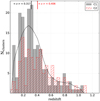 |
Fig. 1 Redshift distribution of XXL C1 (grey histogram) and C2 (red histogram) clusters at z < 1.5, and of the C1 random objects normalised to the number of XXL C1 clusters (black line). The median redshifts of C1 and C2 clusters are shown at the top of the box. |
 |
Fig. 2 Mass distribution of XXL C1 (grey histogram) and C2 (red histogram) clusters at z < 1.5. The median M500 masses of C1 and C2 clusters are shown at the top of the box. |
3 Measurements
3.1 Fromobserved to comoving coordinates
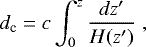
The first step required to measure the 2PCF is to convert observed redshifts into distances. In standard cosmological frameworks, the cosmological redshifts, z, caused by the expansion of space are related to comoving distances, dc, as
 (1)
(1)
where c is the speed of light and H is the Hubble expansion rate. Assuming a flat ΛCDM model, we have
![Mathematical equation: \begin{equation*} H = H_0\left[{\mathrm \Omega}_{\textrm{M}}(1+z)^3+(1-{\mathrm \Omega}_{\textrm{M}})\right]^{1/2} \; .\end{equation*}](/articles/aa/full_html/2018/12/aa33238-18/aa33238-18-eq7.png) (2)
(2)
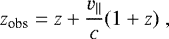
The observed redshift, zobs, is related to the cosmological value by the relation (neglecting redshift errors and second-order corrections)
 (3)
(3)
where v∥ is the line-of-sight component of the centre-of-mass velocity of the source. Since the peculiar velocities are not directly measurable, we compute the comoving distances by substituting z with zobs in Eq. 1. This introduces distortions along the line of sight that are generally called redshift-space distortions. Hereafter, we refer to the redshift-space spatial coordinates using the vector s, whereas we will use r to indicate real-space coordinates.In the following analysis, we will neglect the measurement errors on the observed redshifts since these are subdominant relative to the clustering measurement uncertainties (see e.g. Marulli et al. 2012; Sridhar et al. 2017).
3.2 Two-point correlation function estimator
An efficient way to investigate the large-scale structure of the Universe is to compress its information content into the second-order statistics of extragalactic sources, that is the 2PCF and power spectrum (Totsuji & Kihara 1969; Peebles 1980).
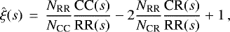
We measure the redshift-space angle-averaged 2PCF using the Landy & Szalay (1993) estimator,
 (4)
(4)
where CC(s), RR (s), and CR (s) are the binned numbers of cluster–cluster, random–random, and cluster–random pairs with distance s ± Δs, while NCC = NC(NC − 1)∕2, NRR = NR(NR − 1)∕2, and NCR = NCNR are the total numbers of cluster–cluster, random–random, and cluster–random pairs in the sample, respectively (see Appendix A.2 for more details). It has been demonstrated that the Landy & Szalay (1993) estimator provides an unbiased estimate of the 2PCF (in the limit NR →∞), with minimum variance. We define the comoving separation associated with each bin as the average cluster pair separation inside the bin, which is more accurate than using the bin centre, especially at large scales, where the bin size is increasingly large (e.g. Zehavi et al. 2011).
3.3 Random catalogue
To estimate the 2PCF via Eq. 4, a random catalogue is required, i.e. a catalogue of randomly distributed points having the same three-dimensional coverage of the data. We adopt the common assumption that the angular and redshift distributions of the tracers are independent and can be treated separately. Following the same methodology applied in Gilli et al. (2005) and Plionis et al. (2018, hereafter XXL Paper XXXII), we construct the random catalogue as follows. We assign angular coordinates (RA–Dec pairs) to the random objects by randomly extracting from the real C1 XXL cluster coordinates, thus reproducing the same angular distribution of the real sources. The redshifts are then assigned by sampling from the Gaussian filtered radial distribution of the XXL clusters (e.g. Marulli et al. 2013). The smoothing is necessary to avoid spurious clustering along the line of sight. We set the smoothing length to σz = 0.1 (see XXL Paper XXXII, for further details). The redshift distribution of the random objects normalised to the number of XXL C1 clusters is shown in Fig. 1.
This method has the advantage of relying on real angular coordinates alone, without any need to model the angular mask. Different assumptions on the angular selection used to construct the random catalogue might impact the measurement at small scales (s ≲ 10h−1 Mpc), although the effect is within the current measurement uncertainties (see Appendix A.4). To minimise the impact of shot noise error due to the finite number of random objects, we construct our random catalogue to be 100 times larger than the XXL cluster sample.
3.4 Covariance matrix
The covariance matrix, Ci,j, which measures the variance and correlation between 2PCF bins, is defined as
 (5)
(5)
where the subscripts i and j run over the 2PCF bins, k refers to the 2PCF of thekth of NR catalogue realisations, and  is the mean 2PCF of the NR samples. The normalisation factor,
  , which takes into account the fact that the NR realisations might not be independent, is
  ,
,  , and
, and  for the subsample, jackknife, and bootstrap methods, respectively (Norberg et al. 2009). We assess the XXL 2PCF covariance matrix with the bootstrap method, using 1000 realisations obtained by resampling galaxy clusters from the original catalogue, with replacement. The impact of this choice is discussed in Appendix A.3.
4 Cosmological analysis
We perform a Bayesian statistical Markov chain Monte Carlo (MCMC) analysis of the 2PCF by sampling the posterior distribution of ΩM, the only free parameter in the assumed flat ΛCDM model considered. As we verified, the current clustering uncertainties do not allow us to consider more general cosmological scenarios, for example models with free dark energy equation of state parameters, by exploiting only the XXL cluster clustering. The joint cosmological analysis of XXL cluster number counts and clustering will be presented in a forthcoming paper.
We consider the commonly used likelihood function,  , defined as
 (6)
(6)
where  is the inverse of the covariance matrix estimated from the data with the bootstrap method (Eq. 5), N is the number of comoving separation bins at which the 2PCF (ξ) is estimated, and the superscripts d and m stand for data and model. The likelihood is estimated at the mean pair separations in each bin (see Sect. 3.2).
The 2PCF model in redshift space, ξm(s), is computedas
![Mathematical equation: \begin{equation*} \xi^{m}(s) = \left[ (b_{\textrm{eff}}\sigma_8)^2 + \frac{2}{3} f\sigma_8 \cdot b_{\textrm{eff}}\sigma_8 + \frac{1}{5}(f\sigma_8)^2 \right] \frac{\xi_{\textrm{DM}}(\alpha r)}{\sigma_8^2} \; ,\end{equation*}](/articles/aa/full_html/2018/12/aa33238-18/aa33238-18-eq19.png) (7)
(7)
where ξDM(r, z) is the real-space dark matter 2PCF, which we estimated by Fourier transforming the power spectrum, PDM(k, z), computed with the software CAMB (Lewis & Bridle 2002). Since the present cluster clustering analysis focuses at sufficiently large scales, the dark matter power spectrum can be safely computed in linear theory,  , with marginal effects on our results. The model depends on two free quantities, fσ8 and beff σ8 (since
  ), and on the reference background cosmology used both to convert angles and redshifts into distances and to estimate the real-space dark matter 2PCF (see e.g. Marulli et al. 2017). The geometric distortions caused by an incorrect assumption of the background cosmology are modelled by the α parameter, i.e. the ratio between the test and fiducial values of the isotropic volume distance, DV, defined as
![Mathematical equation: \begin{equation*} D_{\textrm{V}} \equiv \left[(1+z)^2D_{\textrm{A}}^2\frac{cz}{H}\right]^{1/2} \; ,\end{equation*}](/articles/aa/full_html/2018/12/aa33238-18/aa33238-18-eq22.png) (8)
(8)
where DA is the angular diameter distance (Eisenstein et al. 2005). The α parameter allows us to fit the 2PCF estimated with the fiducial cosmological model without the need to re-measure it for every cosmological model tested in the MCMC.
Equation 7 provides a mapping from real space to redshift space in the distant-observer approximation, assuming that non-linear redshift-space distortion effects can be neglected (Kaiser 1987; Lilje & Efstathiou 1989; McGill 1990; Hamilton 1992; Fisher et al. 1994). This is a reasonable assumption in order to model the clustering of galaxy clusters at the scales considered in this analysis; in other words, the impact of neglecting the Fingersof God effect is marginal, considering current measurement uncertainties (see Marulli et al. 2017, and references therein). The f and beff parameters in Eq. 7 are the linear growth rate and the linear effective bias of the sample, respectively. Specifically, f ≡ dlogδ∕dloga, where a is the dimensionless scale factor and δ is the growing mode linear fractional density perturbation. It can be approximated as  in most cosmological scenarios, with γ ≃ 0.545 in Λ CDM (Wang & Steinhardt 1998; Linder 2005).
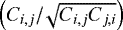
One of the great advantages of using galaxy clusters (instead of galaxies) as density tracers is that we can have an estimate of their total masses, and thus predict their bias given an assumed cosmological model. Following a similar approach to Moscardini et al. (2000b), we account for light-cone effects by estimating the effective bias as the average over the selected cluster pairs,
 (9)
(9)
where  and
and  are the masses of the two XXL clusters of each pair at redshift zi and zj, respectively, assessed by sampling from a Gaussian distribution with standard deviation equal to the given mass uncertainty (see Sect. 2 for details). The linear bias of each cluster, b, is computed with the Tinker et al. (2010) model for M500.
5 Results
5.1 XXL cluster clustering
Figure 3 shows the redshift-space 2PCF of the C1 XXL clusters at z < 1.5. The clustering function is measured, as described in Sect. 3.2, in eight equal logarithmic bins in the comoving separation range 3 < s [h−1 Mpc] < 50. At smaller separations, the clustering signal is not detectable in our data, due to the minimum cluster separation set by the cluster sizes and to the density of the catalogue. On the other hand, at scales larger than those shown in Fig. 3, the signal is dominated by the sample variance, due to the XXL volume. The vertical error bars are the diagonal values of the bootstrap covariance matrix (see Sect. 3.4), while the horizontal error bars represent the standard deviation around the mean pair separation in each bin. The full bootstrap correlation matrix, defined as  (see Eq. 5), is shown in Fig. 4.
5.2 Constraints on ΩM and beff
We model the XXL cluster clustering following the statistical method described in Sect. 4. Figure 3 compares the XXL 2PCF to the best-fit model. Specifically, we show the posterior MCMC median, together with the 68% uncertainty around the median. The fitting analysis is performed in the scale range 10 < r[h−1 Mpc] < 40, where the signal is robust (see Sect. 5.1), though the final results are marginally affected by this choice (see Appendix A.5). The likelihood function is constructed by assuming a flat Λ CDM model with one free parameter ΩM, for which we assume a flat prior in the range [0, 1]. All the other parameters are set to WMAP9 values, with a Gaussian prior on σ8 with mean 0.817 and standard deviation 0.02. The effective bias is a derived parameter that is updated at each MCMC step.
The 1 − 2σ confidence contours of ΩM − beff provided by the MCMC are shown in Fig. 5. We obtain  and
and  , where the best-fit values are the MCMC medians, while the errors are estimated as the 1 − σ of the posterior probability distribution. As expected, this distribution is not symmetric about the mode. The derived best-fit model correlation length, that is the scale for which the redshift-space 2PCF is equal to 1, is s0 = 16 ± 2h−1 Mpc.
Our measurements appear fully consistent with Λ CDM predictions, in agreement with previous cosmological XXL analyses (XXL Paper II; XXL Paper XX; XXL Paper XXV), providing a new and independent confirmation of the standard cosmological framework. Moreover, Fig. 3 demonstrates that the effective bias estimated from the XXL cluster masses via Eq. 9 is consistent with what is expected to match the measured clustering normalisation.
The XXL clustering uncertainties are still too large, however, to allow us to discriminate between WMAP9 and Planck15 cosmologies: both appear consistent with the data. This is shown in Fig. 3, where the measured XXL cluster clustering is compared to the theoretical correlation function computed with Eqs. 7–9, assuming WMAP9 (Hinshaw et al. 2013) and Planck15 (Planck Collaboration XIII 2016) cosmological parameters, as provided in their Table 4 (TT, TE, EE+lowP+lensing), that is Ωm = 0.3121, ΩΛ = 0.6879, Ωb = 0.0488, σ8 = 0.8150, ns = 0.9653. The effective bias values predicted by the Tinker et al. (2010) model in WMAP9 and Planck15 cosmologies, respectively, beff = 2.72 and beff = 2.63, are indicated by lines in Fig. 5. The correlation lengths of WMAP9 and Planck15 cosmologies are s0 = 15.83h−1 Mpc and s0 = 14.81h−1 Mpc, respectively.
Clustering and number counts provide independent complementary probes that can be combined together. As Figs. 3 and 5 demonstrate, this is indeed feasible with XXL data, as the 2PCF signal-to-noise ratio is sufficient at the scales shown. This issue will be addressed in a forthcoming work.
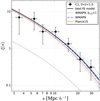 |
Fig. 3 Redshift-space 2PCF of the C1 XXL clusters at z < 1.5 (black dots) compared to the best-fit model, i.e. the median of the MCMC posterior distribution (black solid line). The shaded area shows the 68% uncertainty on the posterior median. The derived best-fit model correlation length is s0 = 16± 2 h−1 Mpc. The red dashed and blue long-dashed lines show the WMAP9 and Planck15 predictions, respectively, computed as described in Sect. 4. Their correlation lengths are s0 = 15.83 h−1 Mpc and s0 = 14.81 h−1 Mpc, respectively. The vertical error bars are the diagonal values of the bootstrap covariance matrix, while the horizontal error bars show the standard deviation around the mean pair separation in each bin. The black dotted line shows the WMAP9 prediction with beff = 1 as a reference. |
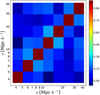 |
Fig. 4 Bootstrap correlation matrix |
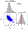 |
Fig. 5 Confidence contours (1 − 2σ) of ΩM − beff provided by the MCMC, as described in Sect. 4 (beff is a derived parameter, the ellipse width corresponds to the deviation of the σ8 Gaussian prior). The histograms (top and bottom right panels) show the posterior distributions of ΩM and beff, respectively.Black and red lines represent WMAP9 and Planck15 predictions, respectively. |
6 Conclusions
We investigated the spatial properties of the largest homogeneous survey of X-ray selected galaxy clusters to date, carried out by the XMM-Newton satellite, and compared the measurements with standard Λ CDM predictions. The main results of this analysis are summarised below:
We measured the 2PCF in redshift space of a sample of 182 X-ray selected galaxy clusters at median redshift ⟨z⟩ = 0.317 and median mass ⟨M500⟩≃ 1.3 × 10¹⁴ M⊙. This is the first time that the clustering of an X-ray selected cluster catalogue at such relatively high redshifts and low masses has been measured.
We modelled the data by performing an MCMC analysis, assuming a flat ΛCDM cosmology. Exploiting the XXL cluster clustering measurements in combination with cluster mass estimates from scaling relations, used to derive the effective bias, we implemented a statistical method independent of the cluster selection function.
We found that the 2PCF of XXL clusters is consistent with the ΛCDM predictions. We obtain
 and
and  . The derived redshift-space correlation length of the C1 XXL clusters is s0 = 16 ± 2h−1 Mpc. This provides an important confirmation of the standard model, which is independent of the cluster number counts and of the other standard cosmological probes, such as the galaxy clustering.
This work also demonstrates that the effective linear bias computed from cluster masses estimated with scaling relations is consistent with the expected cluster clustering normalisation.
Though the current measurement uncertainties are not small enough to discriminate between WMAP9 and Planck15 cosmologies, this work demonstrates the feasibility of a cosmological exploitation of XXL cluster clustering, paving the way for a joint analysis in combination with cluster number counts.
The combination of cluster number counts and clustering is especially powerful when the dark energy equation state parameter is left free. This will thus allow us to constrain a much wider parameter space, as already attempted in XXL Paper XXV with number counts alone. Moreover, in the final combined analysis, we will use the full C1+C2 cluster sample.
The next generation of galaxy surveys, such as the Dark Energy Survey3 (DES; DES Collaboration 2018), the extended Roentgen Survey with an Imaging Telescope Array (eROSITA) satellite mission4 (Merloni et al. 2012), the NASA Wide Field Infrared Space Telescope (WFIRST) mission5 (Spergel et al. 2013), the ESA Euclid mission6 (Laureijs et al. 2011; Amendola et al. 2018), and the Large Synoptic Survey Telescope7 (LSST; Ivezic et al. 2008) will provide increasingly large catalogues of galaxy clusters, extending the current redshift and mass ranges, and eventually providing substantially tighter constraints on cosmological parameters (Borgani & Guzzo 2001; Angulo et al. 2005; Sartoris et al. 2016).
Acknowledgements
XXL is an international project based around an XMM Very Large Programme surveying two 25 deg2 extragalactic fields at a depth of ~6 × 10⁻¹⁵ erg cm−2 s−1 in the [0.5–2] keV band for point-like sources. The XXL website is http://irfu.cea.fr/xxl. Multi-band information and spectroscopic follow-ups of the X-ray sources are obtained through a number of survey programmes, summarised at http://xxlmultiwave.pbworks.com/. We thank L. Chiappetti and M. Roncarelli for helpful comments. F.M. acknowledges support from the grant MIUR PRIN 2015 “Cosmology and Fundamental Physics: Illuminating the Dark Universe with Euclid”. The Saclay group acknowledges long-term support from the Centre National d’Études Spatiales (CNES). S.E. acknowledges financial contributionfrom the contracts NARO15 ASI-INAF I/037/12/0, ASI 2015-046-R.0, and ASI-INAF n.2017-14-H.0. S.A. acknowledges support from Istanbul University with the project number BEK-54547. E.K. thanks CNES and CNRS for support of post-doctoral research.
Appendix A Systematics
This sectionpresents a detailed investigation of all the main systematics that might impact the results of this work. In Appendix A.1 we test the impact of the sample selection. In Appendices A.2 and A.3 we investigate the estimators used in this work to measure the 2PCF and assess its covariance matrix, respectively. In Appendix A.4 we test the method used to construct the random catalogue. In Appendix A.5 we discuss the impact of our modelling assumptions. Finally, in Appendix A.6 we investigate the effect of mass uncertainties.
A.1 Sample selection
The analysis presented in this work was performed using the full sample of 182 C1 XXL clusters at z< 1.5. Here we investigate the impact of this assumption.
Figure A.1 compares the redshift-space 2PCF of C1 XXL clusters in the XXL-N and XXL-S fields separately, and in the whole sample. Given the estimated errors, the three measurements appear consistent with each other; there are no systematic differences.
Figure A.2 shows the 2PCF of the sample comprising both C1 and C2 XXL clusters. As expected, the clustering bias is lower than that for C1 clusters as the mass distribution of the C2 sample is shifted to lower masses (see Fig. 2). Due to the low comoving number density of the C2 cluster sample, the C2 2PCF measurement is highly uncertain, thus limiting our analysis to the comparison between C1 and C1+C2 2PCFs. As shown in Fig. A.2, the 2PCFs of both the C1 and C1+C2 cluster samples are found to be fully consistent with WMAP9 predictions. The 1σ MCMC confidence contours of ΩM − beff are shown in Fig. A.4. We obtain 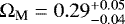 and
and 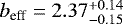 . As expected, the errors on ΩM and beff are slightly smaller than those obtained from the clustering of C1 clusters. To be conservative, we decided to focus the analysis on the C1 sample, which is complete, as discussed in Sect. 2.
A.2 Clustering estimator
The ℓth multipole of the 2PCF is defined as
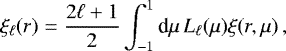 (A.1)
(A.1)
where Lℓ(μ) is the ℓth Legendre polynomial and μ is the cosine of the angle between the galaxy separation and the line of sight. The clustering monopole measured in this work corresponds to ℓ = 0. The signal-to-noise ratio in the higher-order multipoles of the XXL cluster clustering is not sufficient to allow any significant statistical analysis. The clustering multipoles can be computed with the Landy & Szalay (1993) estimator as follows:
 (A.2)
(A.2)
This is the integrated estimator of the 2PCF multipoles. As discussed in Sect. 3.2, the clustering measurements presented in this work have been estimated with a different direct estimator given by Eq. 4, which computes pair counts in 1D scale bins directly. The two estimators coincide when the random pairs do not depend on μ, that is RR (r, μ) = RR(r) (Kazin et al. 2012). This condition is verified in our case, as demonstrated by Fig. A.3, which shows that the 2PCFs measured with the integrated and direct estimators are consistent.
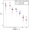 |
Fig. A.1 Comparison between the redshift-space 2PCF of XXL C1 in XXL-N (red diamonds), in XXL-S (blue squares), and in the whole sample (black dots). The number of XXL clusters in each field is reported in parentheses. The error bars are as in Fig. 3. |
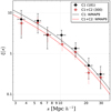 |
Fig. A.2 Comparison between the redshift-space 2PCF of XXL C1 (black dots) and C1+C2 clusters (red diamonds). The black and red lines show the theoretical WMAP9 predictions, computed as described in Sect. 4 for C1 and C1+C2, respectively. The number of C1 and C1+C2 XXL clusters in each field is reported in parentheses. |
The geometric distortions are modelled by the α parameter (see Eq. 7), though they are negligible given the estimated uncertainties (Marulli et al. 2012). The 2PCFs measured assuming either WMAP9 or Planck15 cosmologies are compared in Fig. A.3. We find no significant differences between these measurements to within the estimated errors of the 2PCF. Specifically, we obtain 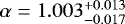 and
and 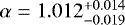 , assuming WMAP9 and Planck15 cosmologies, respectively.
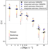 |
Fig. A.3 Comparison between the redshift-space 2PCF of XXL C1 clusters computed with the direct (dots) and integrated (diamonds) estimators, assuming either WMAP9 (solid coloured) or Planck15 (fuzzy coloured, slightly shifted for reasons of clarity). The error bars compare the Poisson, bootstrap, and jackknife estimated errors. |
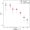 |
Fig. A.4 Comparison between the redshift-space 2PCF of XXL C1 clusters computed with the random catalogue constructed as described in Sect. 3.3 (black dots) and considering the angular mask (red diamonds). |
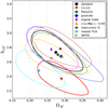 |
Fig. A.5 1σ MCMC confidence contours of ΩM − beff obtained with different assumptions: standard analysis, as described in Sect. 4 – black; considering C1+C2 XXL clusters, instead of C1 only – red; assuming Planck15 as reference cosmology, instead of WMAP9 – green; with jackknife covariance, instead of bootstrap – blue; considering the angular mask to construct the random catalogue, instead of the technique described in Sect. 3.3 – magenta; considering the fitting scale range 1 < r[h−1 Mpc] < 50, instead of 10 < r [h−1 Mpc] < 40 – yellow; doubling thestatistical mass errors – brown; reducing the masses by 20% – cyan; assuming the Sheth et al. (2001) bias model to compute the effective bias of the sample – orange. |
A.3 Covariance matrix
As described in Sect. 3.4, to estimate the XXL 2PCF covariance matrix we used the bootstrap method with 1000 realisations. This number is large enough to assure convergence, as we verified. We compare here this covariance matrix with that obtained with the jackknife method, consisting in subsampling the original catalogue and calculating the 2PCF in all but one subsample. In particular, we apply this procedure by removing each cluster recursively. The error bars shown in Fig. A.3 compare the diagonal values of the jackknife and bootstrap covariance matrices. We also show the estimated Poissonian errors for comparison. The 1σ MCMC confidence contours of ΩM − beff obtained with the jackknife method are shown in Fig. A.4. In this case, we obtain  and
and  , fully in agreement with the results obtained with bootstrap. We adopted the latter as the reference as the XXLbootstrap covariance matrix is smoother, thanks to the larger number of possible resamplings.
A.4 Random catalogue
We test here the impact of the technique adopted to construct the random catalogue. Figure A.4 compares the reference 2PCF with that obtained by considering the XXL angular mask to assign angular coordinates (RA–Dec) to the random objects. The 1σ ΩM − beff contours are shown in Fig. A.5. We have in this case  and
and  . The difference with the reference case is thus within the estimated uncertainties.
A.5 Modelling assumptions
To computethe effective bias of the XXL cluster sample, we assumed the Tinker et al. (2010) model in Eq. 9 (see Sect. 4). To check the impact of this assumption, we repeated our statistical analysis assuming the Sheth et al. (2001) bias, converting the XXL masses to M200. The result, shown in Fig. A.5, is fully consistent with that obtained using the Tinker et al. (2010) model, demonstrating that our conclusions are robust with respect to the bias model adopted. Specifically, we obtain in this case  and
and  .
.
The reference fitting analysis has been performed in the scale range 10 < r[h−1 Mpc] < 40. We show in Fig. A.5 the 1σ ΩM − beff confidence contours obtained by enlarging the fitting range to 1 < r[h−1 Mpc] < 50. The best-fit values are  and
and  , consistent with the reference case.
A.6 Mass uncertainties
As described in Sect. 4, we used the XXL cluster masses to estimate the effective bias of the sample (Eq. 9). The mass measurements depend on the cosmological model. However, given the current clustering uncertainties, this dependence can be safely neglected. To estimate the impact of this assumption on the error budget, we repeated our analysis converting the masses
from the assumed cosmology to the test values at each MCMC step, using Eq. C4 in Sereno & Ettori (2015). The difference in the ΩM best-fit value with respect to the reference case is less than 1% of the estimated error.
The given mass uncertainties considered in our computations include only the statistical errors due to the count rate. To check the impact of this assumption, we performed our statistical analysis by progressively increasing the value of the statistical mass errors. We find that the best-fit value of ΩM shifts systematically to higher values as the mass errors increase, though the impact is marginal. In fact, even doubling the mass errors, the effect is below 1 − σ, as shown in Fig. A.5. In this case, we obtain  and
and  .
.
While the uncertainty on the statistical errors is thus not an issue, systematic errors on cluster masses (see e.g. Eckert et al. 2016, XXL Paper XIII), if present, can more severely impact our cosmological constraints. Specifically, we find a systematic shift to lower values of ΩM for a systematic error that increases the masses. As an illustrative case, in Fig. A.5 we show how our cosmological constraints change if we assume that all the XXL masses are overestimated by 20%. In this case, we obtain  and
and  . This highlights the importance of having a good knowledge of any systematics possibly affecting the cluster mass measurements. Nevertheless, even in this quite extreme case, the effect on ΩM is within 1 − σ.
References
- Abadi, M. G., Lambas, D. G., & Muriel, H. 1998, ApJ, 507, 526 [NASA ADS] [CrossRef] [Google Scholar]
- Adami, C., Giles, P., Koulouridis, E., et al. 2018, A&A, 620, A5 (XXL Survey, XX) [NASA ADS] [CrossRef] [EDP Sciences] [Google Scholar]
- Aihara, H., Arimoto, N., Armstrong, R., et al. 2018, PASJ, 70, S4 [NASA ADS] [Google Scholar]
- Allen, S. W., Evrard, A. E., & Mantz, A. B. 2011, ARA&A, 49, 409 [NASA ADS] [CrossRef] [Google Scholar]
- Amendola, L., Appleby, S., Avgoustidis, A., et al. 2018, Liv. Rev. Rel., 21, 2 [Google Scholar]
- Angulo, R. E., Baugh, C. M., Frenk, C. S., et al. 2005, MNRAS, 362, L25 [NASA ADS] [CrossRef] [Google Scholar]
- Bahcall, N. A., & Soneira, R. M. 1983, ApJ, 270, 20 [NASA ADS] [CrossRef] [Google Scholar]
- Balaguera-Antolínez, A., Sánchez, A. G., Böhringer, H., et al. 2011, MNRAS, 413, 386 [NASA ADS] [CrossRef] [Google Scholar]
- Borgani, S., & Guzzo, L. 2001, Nature, 409, 39 [NASA ADS] [CrossRef] [PubMed] [Google Scholar]
- Borgani, S., Plionis, M., & Kolokotronis, V. 1999, MNRAS, 305, 866 [NASA ADS] [CrossRef] [Google Scholar]
- Chiappetti, A., Fotopoulou, S., Lidman, C., et al. 2018, A&A, 620, A12 (XXL Survey, XXVII) [NASA ADS] [CrossRef] [EDP Sciences] [Google Scholar]
- Colberg, J. M., White, S. D. M., Yoshida, N., et al. 2000, MNRAS, 319, 209 [NASA ADS] [CrossRef] [Google Scholar]
- Collins, C. A., Guzzo, L., Böhringer, H., et al. 2000, MNRAS, 319, 939 [NASA ADS] [CrossRef] [Google Scholar]
- de Jong, J. T. A., Verdoes Kleijn, G. A., Kuijken, K. H., & Valentijn, E. A. 2013, Exp. Astron., 35, 25 [Google Scholar]
- DES Collaboration (Abbott, T. M. C., et al.) 2018, Phys. Rev. D, 98, 043526 [Google Scholar]
- Eckert, D., Ettori, S., Coupon, J., et al. 2016, A&A, 592, A12 (XXL Survey, XIII) [NASA ADS] [CrossRef] [EDP Sciences] [Google Scholar]
- Eisenstein, D. J., Zehavi, I., Hogg, D. W., et al. 2005, ApJ, 633, 560 [NASA ADS] [CrossRef] [Google Scholar]
- Emami, R., Broadhurst, T., Jimeno, P., et al. 2017, ArXiv e-prints [arXiv:1711.05210] [Google Scholar]
- Estrada, J., Sefusatti, E., & Frieman, J. A. 2009, ApJ, 692, 265 [NASA ADS] [CrossRef] [Google Scholar]
- Fisher, K. B., Scharf, C. A., & Lahav, O. 1994, MNRAS, 266, 219 [NASA ADS] [CrossRef] [Google Scholar]
- Gilli, R., Daddi, E., Zamorani, G., et al. 2005, A&A, 430, 811 [NASA ADS] [CrossRef] [EDP Sciences] [Google Scholar]
- Guzzo, L., Scodeggio, M., Garilli, B., et al. 2014, A&A, 566, A108 [NASA ADS] [CrossRef] [EDP Sciences] [Google Scholar]
- Hamilton, A. J. S. 1992, ApJ, 385, L5 [NASA ADS] [CrossRef] [Google Scholar]
- Hinshaw, G., Larson, D., Komatsu, E., et al. 2013, ApJS, 208, 19 [NASA ADS] [CrossRef] [Google Scholar]
- Hong, T., Han, J. L., Wen, Z. L., Sun, L., & Zhan, H. 2012, ApJ, 749, 81 [NASA ADS] [CrossRef] [Google Scholar]
- Hong, T., Han, J. L., & Wen, Z. L. 2016, ApJ, 826, 154 [NASA ADS] [CrossRef] [Google Scholar]
- Hütsi, G. 2010, MNRAS, 401, 2477 [NASA ADS] [CrossRef] [Google Scholar]
- Ivezic, Z., Kahn, S. M., Tyson, J. A., et al. 2008, ArXiv e-prints [arXiv:0805.2366] [Google Scholar]
- Kaiser, N. 1987, MNRAS, 227, 1 [NASA ADS] [CrossRef] [Google Scholar]
- Kaiser, N., Burgett, W., Chambers, K., et al. 2010, in Ground-based and Airborne Telescopes III, Proc. SPIE 7733, 77330E [CrossRef] [Google Scholar]
- Kazin, E. A., Sánchez, A. G., & Blanton, M. R. 2012, MNRAS, 419, 3223 [NASA ADS] [CrossRef] [Google Scholar]
- Klypin, A. A., & Kopylov, A. I. 1983, Sov. Astron. Lett., 9, 41 [NASA ADS] [Google Scholar]
- Lahav, O., Fabian, A. C., Edge, A. C., & Putney, A. 1989, MNRAS, 238, 881 [NASA ADS] [CrossRef] [Google Scholar]
- Landy, S. D., & Szalay, A. S. 1993, ApJ, 412, 64 [NASA ADS] [CrossRef] [Google Scholar]
- Laureijs, R., Amiaux, J., Arduini, S., et al. 2011, ArXiv e-prints [arXiv:1110.3193] [Google Scholar]
- Lewis, A., & Bridle, S. 2002, Phys. Rev. D, 66, 103511 [NASA ADS] [CrossRef] [Google Scholar]
- Lieu, M., Smith, G. P., Giles, P. A., et al. 2016, A&A, 592, A4 (XXL Survey, IV) [NASA ADS] [CrossRef] [EDP Sciences] [Google Scholar]
- Lilje, P. B., & Efstathiou, G. 1989, MNRAS, 236, 851 [NASA ADS] [CrossRef] [Google Scholar]
- Linder, E. V. 2005, Phys. Rev. D, 72, 043529 [NASA ADS] [CrossRef] [MathSciNet] [Google Scholar]
- Majumdar, S.,& Mohr, J. J. 2004, ApJ, 613, 41 [NASA ADS] [CrossRef] [Google Scholar]
- Mana, A., Giannantonio, T., Weller, J., et al. 2013, MNRAS, 434, 684 [NASA ADS] [CrossRef] [Google Scholar]
- Marulli, F., Bianchi, D., Branchini, E., et al. 2012, MNRAS, 426, 2566 [NASA ADS] [CrossRef] [Google Scholar]
- Marulli, F., Veropalumbo, A., & Moresco, M. 2016, Astron. Comput., 14, 35 [NASA ADS] [CrossRef] [Google Scholar]
- Marulli, F., Veropalumbo, A., Moscardini, L., Cimatti, A., & Dolag, K. 2017, Astron. Astrophys., 599, A106 [NASA ADS] [CrossRef] [EDP Sciences] [Google Scholar]
- Marulli, F., Bolzonella, M., Branchini, E., et al. 2013, A&A, 557, A17 [NASA ADS] [CrossRef] [EDP Sciences] [Google Scholar]
- McGill, C. 1990, MNRAS, 242, 428 [NASA ADS] [CrossRef] [Google Scholar]
- Merloni, A., Predehl, P., Becker, W., et al. 2012, ArXiv e-prints [arXiv:1209.3114] [Google Scholar]
- Miller, C. J., & Batuski, D. J. 2001, ApJ, 551, 635 [NASA ADS] [CrossRef] [Google Scholar]
- Mo, H. J., & White, S. D. M. 1996, MNRAS, 282, 347 [NASA ADS] [CrossRef] [Google Scholar]
- Moscardini, L., Matarrese, S., De Grandi, S., & Lucchin, F. 2000a, MNRAS, 314, 647 [NASA ADS] [CrossRef] [Google Scholar]
- Moscardini, L., Matarrese, S., Lucchin, F., & Rosati, P. 2000b, MNRAS, 316, 283 [CrossRef] [Google Scholar]
- Nichol, R. C., Briel, O. G., & Henry, J. P. 1994, MNRAS, 267, 771 [NASA ADS] [CrossRef] [Google Scholar]
- Norberg, P., Baugh, C. M., Gaztañaga, E., & Croton, D. J. 2009, MNRAS, 396, 19 [NASA ADS] [CrossRef] [Google Scholar]
- Pacaud, F., Clerc, N., Giles, P. A., et al. 2016, A&A, 592, A2 (XXL Survey, II) [NASA ADS] [CrossRef] [EDP Sciences] [Google Scholar]
- Pacaud, F., Pierre, M., Melin, J.-B., et al. 2018, A&A, 620, A10 (XXL Survey, XXV) [Google Scholar]
- Peebles, P. J. E. 1980, The Large-scale Structure of the Universe [Google Scholar]
- Pierre, M., Pacaud, F., Adami, C., et al. 2016, A&A, 592, A1 (XXL Survey, I) [NASA ADS] [CrossRef] [EDP Sciences] [Google Scholar]
- Planck Collaboration XIII 2016, A&A, 594, A13 [NASA ADS] [CrossRef] [EDP Sciences] [Google Scholar]
- Plionis, M., Koutoulidis, L., Koulouridis, E., et al. 2018, A&A, 620, A17 (XXL Survey, XXXII) [NASA ADS] [CrossRef] [EDP Sciences] [Google Scholar]
- Retzlaff, J., Borgani, S., Gottlöber, S., Klypin, A., & Müller, V. 1998, New Astron. Rev., 3, 631 [NASA ADS] [CrossRef] [Google Scholar]
- Romer, A. K., Collins, C. A., Böhringer, H., et al. 1994, Nature, 372, 75 [NASA ADS] [CrossRef] [Google Scholar]
- Sartoris, B., Biviano, A., Fedeli, C., et al. 2016, MNRAS, 459, 1764 [NASA ADS] [CrossRef] [Google Scholar]
- Schuecker, P., Böhringer, H., Guzzo, L., et al. 2001, A&A, 368, 86 [NASA ADS] [CrossRef] [EDP Sciences] [Google Scholar]
- Schuecker, P., Böhringer, H., Collins, C. A., & Guzzo, L. 2003, A&A, 398, 867 [NASA ADS] [CrossRef] [EDP Sciences] [Google Scholar]
- Sereno, M., & Ettori, S. 2015, MNRAS, 450, 3633 [NASA ADS] [CrossRef] [Google Scholar]
- Sereno, M., Veropalumbo, A., Marulli, F., et al. 2015, MNRAS, 449, 4147 [NASA ADS] [CrossRef] [Google Scholar]
- Sheth, R. K., Mo, H. J., & Tormen, G. 2001, MNRAS, 323, 1 [NASA ADS] [CrossRef] [Google Scholar]
- Spergel, D., Gehrels, N., Breckinridge, J., et al. 2013, ArXiv e-prints [arXiv:1305.5422] [Google Scholar]
- Sridhar, S., Maurogordato, S., Benoist, C., Cappi, A., & Marulli, F. 2017, A&A, 600, A32 [NASA ADS] [CrossRef] [EDP Sciences] [Google Scholar]
- Suto, Y., Yamamoto, K., Kitayama, T., & Jing, Y. P. 2000, ApJ, 534, 551 [NASA ADS] [CrossRef] [Google Scholar]
- Tinker, J. L., Robertson, B. E., Kravtsov, A. V., et al. 2010, ApJ, 724, 878 [NASA ADS] [CrossRef] [Google Scholar]
- Totsuji, H., & Kihara, T. 1969, PASJ, 21, 221 [NASA ADS] [Google Scholar]
- Veropalumbo, A., Marulli, F., Moscardini, L., Moresco, M., & Cimatti, A. 2014, MNRAS, 442, 3275 [NASA ADS] [CrossRef] [Google Scholar]
- Veropalumbo, A., Marulli, F., Moscardini, L., Moresco, M., & Cimatti, A. 2016, MNRAS, 458, 1909 [NASA ADS] [CrossRef] [Google Scholar]
- Wang, L., & Steinhardt, P. J. 1998, ApJ, 508, 483 [NASA ADS] [CrossRef] [Google Scholar]
- York, D. G., Adelman, J., Anderson, Jr., J. E., et al. 2000, Astron. J., 120, 1579 [NASA ADS] [CrossRef] [Google Scholar]
- Zehavi, I., Zheng, Z., Weinberg, D. H., et al. 2011, ApJ, 736, 59 [NASA ADS] [CrossRef] [Google Scholar]
Specifically, we use the CosmoBolognaLib V4.1, which implements OpenMP parallel algorithms both to measure the 2PCF (Sect. 3) and to perform Markov chain Monte Carlo sampling (Sect. 4). The CosmoBolognaLib is entirely implemented in C++ to provide a high-performance back end for all the computationally expensive tasks, while also supporting their use in Python to exploit the higher-level abstraction of this language. The software and its documentation are freely available at the GitHub repository: https://github.com/federicomarulli/CosmoBolognaLib.
M500 is defined as the mass within radius R500, which is the radius enclosing a mean density of 500 times the critical density at the redshift of the cluster.
All Figures
|
Fig. 1 Redshift distribution of XXL C1 (grey histogram) and C2 (red histogram) clusters at z < 1.5, and of the C1 random objects normalised to the number of XXL C1 clusters (black line). The median redshifts of C1 and C2 clusters are shown at the top of the box. |
| In the text | |
|
Fig. 2 Mass distribution of XXL C1 (grey histogram) and C2 (red histogram) clusters at z < 1.5. The median M500 masses of C1 and C2 clusters are shown at the top of the box. |
| In the text | |
|
Fig. 3 Redshift-space 2PCF of the C1 XXL clusters at z < 1.5 (black dots) compared to the best-fit model, i.e. the median of the MCMC posterior distribution (black solid line). The shaded area shows the 68% uncertainty on the posterior median. The derived best-fit model correlation length is s0 = 16± 2 h−1 Mpc. The red dashed and blue long-dashed lines show the WMAP9 and Planck15 predictions, respectively, computed as described in Sect. 4. Their correlation lengths are s0 = 15.83 h−1 Mpc and s0 = 14.81 h−1 Mpc, respectively. The vertical error bars are the diagonal values of the bootstrap covariance matrix, while the horizontal error bars show the standard deviation around the mean pair separation in each bin. The black dotted line shows the WMAP9 prediction with beff = 1 as a reference. |
| In the text | |
|
Fig. 4 Bootstrap correlation matrix |
| In the text | |
|
Fig. 5 Confidence contours (1 − 2σ) of ΩM − beff provided by the MCMC, as described in Sect. 4 (beff is a derived parameter, the ellipse width corresponds to the deviation of the σ8 Gaussian prior). The histograms (top and bottom right panels) show the posterior distributions of ΩM and beff, respectively.Black and red lines represent WMAP9 and Planck15 predictions, respectively. |
| In the text | |
|
Fig. A.1 Comparison between the redshift-space 2PCF of XXL C1 in XXL-N (red diamonds), in XXL-S (blue squares), and in the whole sample (black dots). The number of XXL clusters in each field is reported in parentheses. The error bars are as in Fig. 3. |
| In the text | |
|
Fig. A.2 Comparison between the redshift-space 2PCF of XXL C1 (black dots) and C1+C2 clusters (red diamonds). The black and red lines show the theoretical WMAP9 predictions, computed as described in Sect. 4 for C1 and C1+C2, respectively. The number of C1 and C1+C2 XXL clusters in each field is reported in parentheses. |
| In the text | |
|
Fig. A.3 Comparison between the redshift-space 2PCF of XXL C1 clusters computed with the direct (dots) and integrated (diamonds) estimators, assuming either WMAP9 (solid coloured) or Planck15 (fuzzy coloured, slightly shifted for reasons of clarity). The error bars compare the Poisson, bootstrap, and jackknife estimated errors. |
| In the text | |
|
Fig. A.4 Comparison between the redshift-space 2PCF of XXL C1 clusters computed with the random catalogue constructed as described in Sect. 3.3 (black dots) and considering the angular mask (red diamonds). |
| In the text | |
|
Fig. A.5 1σ MCMC confidence contours of ΩM − beff obtained with different assumptions: standard analysis, as described in Sect. 4 – black; considering C1+C2 XXL clusters, instead of C1 only – red; assuming Planck15 as reference cosmology, instead of WMAP9 – green; with jackknife covariance, instead of bootstrap – blue; considering the angular mask to construct the random catalogue, instead of the technique described in Sect. 3.3 – magenta; considering the fitting scale range 1 < r[h−1 Mpc] < 50, instead of 10 < r [h−1 Mpc] < 40 – yellow; doubling thestatistical mass errors – brown; reducing the masses by 20% – cyan; assuming the Sheth et al. (2001) bias model to compute the effective bias of the sample – orange. |
| In the text | |
Current usage metrics show cumulative count of Article Views (full-text article views including HTML views, PDF and ePub downloads, according to the available data) and Abstracts Views on Vision4Press platform.
Data correspond to usage on the plateform after 2015. The current usage metrics is available 48-96 hours after online publication and is updated daily on week days.
Initial download of the metrics may take a while.