| Issue |
A&A
Volume 697, May 2025
|
|
|---|---|---|
| Article Number | A140 | |
| Number of page(s) | 12 | |
| Section | Cosmology (including clusters of galaxies) | |
| DOI | https://doi.org/10.1051/0004-6361/202554608 | |
| Published online | 20 May 2025 | |
The robustness of cluster clustering covariance calibration
1
Ludwig-Maximilians-University, Schellingstrasse 4, 80799 Munich, Germany
2
INAF – Osservatorio Astronomico di Trieste, Via G. B. Tiepolo 11, 34143 Trieste, Italy
3
IFPU, Institute for Fundamental Physics of the Universe, via Beirut 2, 34151 Trieste, Italy
4
INFN, Sezione di Trieste, Via Valerio 2, 34127 Trieste TS, Italy
5
ICSC – Centro Nazionale di Ricerca in High Performance Computing, Big Data e Quantum Computing, Via Magnanelli 2, Bologna, Italy
6
Dipartimento di Fisica – Sezione di Astronomia, Università di Trieste, Via Tiepolo 11, Trieste 34131, Italy
⋆ Corresponding authors: This email address is being protected from spambots. You need JavaScript enabled to view it.
, This email address is being protected from spambots. You need JavaScript enabled to view it.
Received:
18
March
2025
Accepted:
1
April
2025
Abstract
Ongoing and upcoming wide-field surveys at different wavelengths will measure the distribution of galaxy clusters with unprecedented precision, demanding accurate models for the two-point correlation function (2PCF) covariance. In this work we assessed a semi-analytical framework for the cluster 2PCF covariance that employs three nuisance parameters to account for non-Poissonian shot noise, residual uncertainties in the halo bias model, and sub-leading noise terms. We calibrated these parameters on a suite of fast approximate simulations generated by PINOCCHIO as well as full N-body simulations from OpenGADGET3. We demonstrate that PINOCCHIO can reproduce the 2PCF covariance measured in OpenGADGET3 at the few percent level, provided the mass functions are carefully rescaled. Resolution tests confirm that high particle counts are necessary to capture shot-noise corrections, especially at high redshifts. We performed the parameter calibration across multiple cosmological models, showing that one of the nuisance parameters, the non-Poissonian shot-noise correction (α), depends mildly on the amplitude of matter fluctuations (σ8). In contrast, the remaining two parameters, β, which controls the bias correction, and γ, which controls the secondary shot-noise correction, exhibit more significant variation with redshift and halo mass. Overall, our results underscore the importance of calibrating covariance models on realistic mock catalogs that replicate the selection function of forthcoming surveys and highlight that approximate methods, when properly tuned, can effectively complement full N-body simulations for precision cluster cosmology.
Key words: methods: numerical / methods: statistical / galaxies: clusters: general / cosmology: theory / large-scale structure of Universe
© The Authors 2025
 Open Access article, published by EDP Sciences, under the terms of the Creative Commons Attribution License (https://creativecommons.org/licenses/by/4.0), which permits unrestricted use, distribution, and reproduction in any medium, provided the original work is properly cited.
This article is published in open access under the Subscribe to Open model. This email address is being protected from spambots. You need JavaScript enabled to view it. to support open access publication.
1. Introduction
Galaxy clusters, the most massive virialized objects in the Universe, have long been recognized as powerful probes of cosmology thanks to their sensitivity to both the geometry and growth of large-scale structure (see, e.g., Allen et al. 2011; Kravtsov & Borgani 2012). Traditional cluster studies have focused on the abundance of these systems and their variation with redshift to constrain cosmological parameters such as the matter density parameter (Ωm) and the amplitude of matter fluctuations (σ8; Borgani et al. 2001; Vikhlinin et al. 2009; Planck Collaboration XX 2014; Planck Collaboration XXIV 2016; Bocquet et al. 2019; Costanzi et al. 2021). Nonetheless, the two-point correlation function (2PCF) of clusters is also a promising probe, as it is highly sensitive to the bias–mass relation and can help break degeneracies that affect cluster abundance studies (Schuecker et al. 2003; Majumdar & Mohr 2004; Sartoris et al. 2016; Marulli et al. 2018; Fumagalli et al. 2024). When the 2PCF is combined with other observables such as number counts or weak lensing, it can provide tighter cosmological constraints while helping calibrate mass–observable relations (Mana et al. 2013; To 2021; Castro et al. 2020).
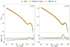 |
Fig. 1. Top: Comparison of the PINOCCHIO 2PCF measured on the comoving box from the original mocks (Fumagalli et al. 2021) and our new high-resolution C0. The new and original simulations assume different but similar cosmologies. We present only the theoretical expectation for the C0 cosmology for better figure readability. Bottom: Residual between the measured 2PCF and the respective theoretical expectation. The shaded gray area denotes the region within a relative difference of less than 10 percent. |
An accurate assessment of cosmological constraints from cluster clustering hinges on a robust model for the covariance of the 2PCF. In contrast to the comparatively simpler case of cluster number counts (e.g., Hu & Kravtsov 2003; Fumagalli et al. 2021), the covariance of the 2PCF of clusters requires additional parameters to reproduce the results of numerical simulations, due to non-Gaussianities and nonlinearities (Euclid Collaboration: Fumagalli et al. 2024). Recent works have demonstrated that, for photometrically selected cluster surveys similar to the one anticipated from Euclid (Laureijs et al. 2011), a Gaussian model with standard Poisson noise can fail to capture all relevant contributions in the covariance. Consequently, one must introduce ad hoc corrections, calibrated against simulations, that take into account non-Gaussian effects and the specific statistical weight of cluster samples.
In previous studies, fast approximate simulations such as those produced by the PINOCCHIO algorithm (Monaco et al. 2002, 2013; Munari et al. 2017) have proven valuable for modeling the 2PCF covariance. By generating a large number of past-light-cone realizations, it is possible to calibrate the extra parameters associated with the analytical covariance to match measurements from mock cluster catalogs (e.g., Fumagalli et al. 2022). In Euclid Collaboration: Fumagalli et al. (2024) such calibrations were carried out at fixed cosmology, thus leaving open the question of whether the best-fit parameters for the covariance depend on the underlying cosmological model. Moreover, although approximate methods like PINOCCHIO can reproduce many large-scale structure statistics with remarkable efficiency, they inevitably involve simplifying assumptions in treating nonlinear gravitational collapse. It is therefore crucial to establish whether the covariance parameters calibrated on PINOCCHIO differ significantly from those obtained from full N-body simulations.
Among the forthcoming wide-field surveys, the Vera C. Rubin Observatory's Legacy Survey of Space and Time1 (LSST; LSST Science Collaborations 2009), the third generation of the South Pole Telescope2 (SPT-3G; Benson et al. 2014), eROSITA3 (Predehl et al. 2021), the Square Kilometre Array4 (SKA; Maartens et al. 2015), the Dark Energy Spectroscopic Instrument (DESI5; DESI Collaboration 2016), the Nancy Grace Roman Space Telescope6 (Spergel et al. 2015), and Euclid7 (Euclid Collaboration: Mellier et al. 2025) are poised to deliver measurements of summary statistics of the distribution of galaxy clusters with unprecedented statistical precision. These datasets will demand more accurate covariance models to fully exploit the cosmological information encoded in cluster clustering. The scope of this study is therefore twofold. First, we investigated the cosmology dependence of the calibrated parameters that enter the covariance model for the cluster 2PCF. Second, we compared the parameters extracted from PINOCCHIO-based mocks with those calibrated on higher-fidelity N-body simulations. This analysis directly tests the robustness of the covariance modeling for future surveys such as Euclid, which is expected to deliver a photometric cluster catalog of unprecedented size and redshift coverage. Ultimately, a more reliable covariance prescription will improve cosmological constraints from cluster clustering and deepen our understanding of systematic uncertainties.
In Sect. 2 we present the theoretical framework for the 2PCF, the semi-analytical covariance model, and the procedure for fitting parameters. In Sect. 3 we summarize the simulations used for our covariance calibration and introduce the cluster catalogs derived from PINOCCHIO and N-body simulations. We compare and discuss our results in Sect. 4, where we also quantify the impact of cosmology dependence and the differences between approximate and full N-body calibrations. We discuss the implications of our results in Sect. 5. Finally, we draw our conclusions in Sect. 6, emphasizing the implications of our findings for the cosmological exploitation of cluster clustering in forthcoming wide-field surveys.
2. Covariance formalism
This section concisely summarizes the semi-analytical model for the real-space 2PCF covariance of galaxy clusters (or halos). A more extensive derivation and validation can be found in Meiksin & White (1999) and Euclid Collaboration: Fumagalli et al. (2024), with additional details on numerical calibrations provided by Fumagalli et al. (2022).
2.1. Baseline model and notation
The core of the 2PCF covariance model starts from the halo power spectrum covariance in Fourier space, which contains both Gaussian and non-Gaussian contributions (see, e.g., Meiksin & White 1999; Scoccimarro et al. 1999). In real space, the halo 2PCF at a given redshift z and separation r can be expressed as
 (1)
(1)
where Ph(k, z) is the halo power spectrum, and j0 is the spherical Bessel function of order zero. On large (linear) scales, the halo power spectrum can be approximated by
 (2)
(2)
where  is the effective linear bias of halos obtained by averaging the linear bias model presented in Euclid Collaboration: Castro et al. (2024) weighting it by mass according to the halo mass function (HMF; Euclid Collaboration: Castro et al. 2023), and Pm(k, z) is the linear matter power spectrum. When calculating the covariance, the discrete nature of halos introduces an additional source of randomness that is independent of the clustering of the matter field. This effect, known as shot noise, is accounted for by adding a
  term to the power spectrum of Eq. (2). Such a term provides the leading-order Poisson shot-noise component for a point distribution whose redshift-dependent comoving mean number density is
  . When transforming to configuration space and integrating over redshift bins, one obtains a baseline model (Gaussian plus lowest-order shot noise) for the 2PCF covariance (see Cohn 2006; Hu & Kravtsov 2003):
![Mathematical equation: $$ \begin{aligned} C_{ij}(z) \;=\;& \frac {2}{V_z}\, \int \frac {k^2\, {\textrm {d}}k}{2\pi ^2}\,\Biggl [P_{{\textrm {h}}}(k,z) + \frac {1}{{\bar {n}}(z)}\Biggr ]^2\,W_{i}(k)\,W_{j}(k)\,\\ &+ \frac {2}{V_z} \int \frac {{\textrm {d}} k\,k^2}{2 \pi ^2} {{\bar {b}}\,}^2 P_{\rm m}(k)\,\Biggl [\frac {1}{{{\bar {n}}}(z)}\Biggr ]^2 \, W_j(k) \ \frac {\delta _{ij}}{V_i}. \end{aligned} $$](/articles/aa/full_html/2025/05/aa54608-25/aa54608-25-eq6.gif) (3)
(3)
Here Vz is the comoving volume in the redshift slice, Wi(k) is the window function for the i-th separation bin, and the sub-leading terms account for additional shot-noise corrections. In principle, one can include contributions from higher-order correlation terms (Meiksin & White 1999; Scoccimarro et al. 1999) and from super-sample covariance (Takada & Hu 2013) for more accuracy, but they often add significant complexity and require the calibration of nuisance parameters.
2.2. Limitations of the baseline model
Equation (3) was shown to underestimate the total covariance when compared to simulations (see, for instance, Euclid Collaboration: Fumagalli et al. 2024). Known limitations include:
-
–
Non-Poissonian shot noise: The simple
 term in general does not capture the non-Poissonian nature of the sampling of the underlying density field provided by the biased halo distribution, especially at high masses or high redshifts;
 -
–
Inaccurate bias prescription: Linear bias formulae sometimes introduce residual offsets in amplitude or scale dependence;
-
–
Neglected higher-order terms: Bispectrum and trispectrum contributions can be non-negligible for cluster-scale halos, particularly if the survey volume or mass threshold is such that the number density is small.
These effects can lead to a mismatch of up to tens of percent between the baseline model and numerical simulations (Euclid Collaboration: Fumagalli et al. 2024).
The halo bias and shot-noise terms in the covariance can be rescaled by empirical parameters that effectively absorb the missing (or inaccurately modeled) contributions to correct for these discrepancies. In practice, one modifies Eq. (3) as
![Mathematical equation: $$ \begin{aligned}C_{ij}^{\textrm {fit}}(z) \;=\;& \frac {2}{V_z} \int \!\frac {k^2\,{\textrm {d}}k}{2\pi ^2} \Biggl [\bigl (\beta \, {\bar {b}}\bigr )^2 P_{{\textrm {m}}}(k,z) + \bigl (1 + \alpha \bigr )\frac {1}{{\bar {n}}(z)}\Biggr ]^2 W_i(k)\,W_j(k)\,\\ &+ \frac {2}{V_z} \int \frac {{\textrm {d}} k\,k^2}{2 \pi ^2} \bigl (\beta \, {\bar {b}}\bigr )^2 P_{\rm m}(k)\,\Biggl [\bigl (1 + \gamma \bigr )\frac {1}{{\bar {n}}(z)}\Biggr ]^2 \, W_j(k) \ \frac {\delta _{ij}}{V_i}, \end{aligned} $$](/articles/aa/full_html/2025/05/aa54608-25/aa54608-25-eq8.gif) (4)
(4)
where α, β, and γ are treated as nuisance parameters to be calibrated against a suite of mock halo catalogs extracted from simulations. In summary,
-
–
β corrects for residual bias errors (i.e., an over- or underestimation of
 ),
), -
–
α adjusts the main shot-noise amplitude to account for non-Poissonian behavior and missing non-Gaussian terms,
-
–
γ modifies a secondary shot-noise contribution in the diagonal terms, mostly contributing at small scales.
By fitting {α, β, γ} to simulation measurements, one can achieve better than 10 percent agreement between the analytical covariance and the fully numerical result, at least for a fixed cosmology (Euclid Collaboration: Fumagalli et al. 2024).
2.3. Fitting procedure
The fitting method, presented in Fumagalli et al. (2022), is designed to efficiently construct a reliable covariance matrix by constraining a model with free parameters. The procedure begins by defining a model covariance matrix, which may be incomplete or approximate, and introducing free parameters to capture unknown or uncertain contributions to the covariance. The model is then constrained by maximizing a Gaussian likelihood function evaluated at a fixed fiducial cosmology, with the free parameters of the covariance matrix as fitting variables. The best-fit covariance is then obtained by ensuring that the χ2 values from the model match the theoretical distribution for the observed data: the correct covariance should provide χ2 values from each simulation that follow a χ2 distribution. The key advantage of this approach is that it requires significantly fewer simulations than traditional methods for covariance estimation – typically around 102 simulations, compared to the thousands (∼103−104) usually needed for a full, accurate numerical covariance matrix.
3. Methodology
We generated halo catalogs using two different approaches: large N-body simulations with OpenGADGET3 and approximate simulations with PINOCCHIO. Below, we describe the setup of each simulation suite, summarize the resulting halo catalogs used in our analyses, and describe the procedure to measure the 2PCF and power spectra.
3.1. N-body simulations
N-body simulations are carried out with the Tree-PM OpenGADGET3 N-body code (Dolag et al. in prep.). OpenGADGET3 represents an evolution of the GADGET3 code, which in turn provides an improvement of the publicly available GADGET2 code (Springel 2005). It adopts a mixed MPI–OpenMP parallelization that allows the code to optimally exploit the parallelism offered by computing nodes with a significant amount of shared memory. Our simulations adopt a flat Λ cold dark matter cosmology that we refer to as C0 throughout this paper and present the specific cosmological parameter values in Table 1.
Different cosmological parameters considered in this work.
We ran 120 realizations of this cosmology, each following 20483 dark matter particles in a comoving, cubic box of side length 3870 h−1 Mpc. The gravitational softening length was chosen to be one-fortieth of the mean inter-particle spacing, ensuring that the HMF and large-scale clustering are well resolved across the range of halo masses of interest (typically M≳1014 h−1 M⊙). The initial conditions for 100 of these realizations were generated with the MONOFONIC code (Michaux et al. 2021). The remaining 20 adopted the same Fourier amplitudes and phases used for a subset of the PINOCCHIO simulations (see Sect. 3.2) to facilitate a direct comparison.
Each OpenGADGET3 simulation was evolved from z = 24 down to z = 0, outputting snapshots at various intermediate redshifts z∈{0.0, 0.5, 1.0, 2.0}. We identified halos in each snapshot using SUBFIND (Springel et al. 2001, 2021; Dolag et al. 2009). SUBFIND determines halos by first executing a parallel friends-of-friends (FOF) with linking length set to 0.2 (see Davis et al. 1985, for instance) and then assigning its center to the position of the particle with the lowest potential. The simulation outputs provide a set of comoving box halo catalogs for each realization.
3.2. Approximate simulations: PINOCCHIO
We also used the Lagrangian perturbation theory-based PINOCCHIO code (Monaco et al. 2002, 2013; Munari et al. 2017) to produce halo catalogs in a more computationally efficient manner, enabling exploration of multiple cosmological models and a large number of realizations. This work complements the original set of PINOCCHIO catalogs presented in Fumagalli et al. (2021) and serves as a basis for comparison. We generated 20 PINOCCHIO realizations using the C0 cosmological parameters and the same mass resolution as our OpenGADGET3 simulations. These runs employ identical box size, particle number (20483), and initial Fourier mode amplitudes and phases, enabling a direct one-to-one comparison of halo statistics between PINOCCHIO and full N-body catalogs under identical initial conditions. In contrast, the original set assumed Ωm, 0 = 0.30711 and used a grid of 21603 elements, which led to a mass resolution difference of roughly 20 percent.
We further exploited PINOCCHIO's efficiency to create an extensive suite of 900 comoving box simulations covering nine additional cosmological models, labeled originally C0 through C8 in Euclid Collaboration: Castro et al. (2023). Each cosmology has 100 realizations, each with 30723 dark matter particles in a box the same size as the previously presented simulations. These simulations broadly sample parameter space, enabling us to study how our covariance model (and its nuisance parameters) might vary across different cosmological parameters.
In addition to comoving outputs, PINOCCHIO can generate halo catalogs on past light cones. We constructed such cones with a 60deg aperture. These light-cone catalogs mimic in a simplistic way the typical sky coverage of future wide-field cluster survey footprints on an idealized uniform and unmasked coverage.
3.3. Summary of simulation sets
Overall, we assembled:
-
900 high-resolution PINOCCHIO realizations spanning nine distinct cosmological models (C0–C8), each with 30723 particles and box size of 3870 h−1 Mpc, for robust exploration of cosmology dependence. We further generated catalogs in the past light cone of 60 deg aperture for these simulations, mimicking wide-field cluster surveys;
-
100 low-resolution N-body realizations at the C0 cosmology with the same box size and 20483 particles;
-
20 PINOCCHIO and 20 N-body realizations were generated at low resolution (20483 particles) assuming the C0 cosmology. The phases and amplitudes of the initial Fourier modes in the two simulations were identical, thereby allowing straightforward comparisons of halo statistics within comoving boxes of identical size. Because the PINOCCHIO and OpenGADGET3 runs in this sub-set share the same initial conditions, the sample noise in the relative statistics between the two codes is greatly reduced;
-
100 PINOCCHIO realizations from the set used in Fumagalli et al. (2021), Euclid Collaboration: Fumagalli et al. (2024), with low resolution similar to the N-body set. These mocks, labeled as “original” set, have the same box size and a cosmology similar to C0. This last set will serve as a reference for comparison with previous works.
The combination of full N-body and approximate PINOCCHIO simulations at matched initial conditions and over multiple cosmologies allows us to assess the robustness of the 2PCF covariance model, as well as the cosmology dependence of the nuisance parameters introduced in Sect. 2.
3.4. Post-processing
3.4.1. Mass rescaling
PINOCCHIO has been calibrated to reproduce within a few percent the FOF-based HMF presented by Watson et al. (2013). To instead reproduce our adopted model for the HMF (Euclid Collaboration: Castro et al. 2023) while keeping the sample variance and shot noise for each simulation, we implemented the rescaling of the halo masses as proposed by Fumagalli et al. (2021) on all PINOCCHIO outputs. To obtain a fair comparison in Sect. 4.1, we also rescaled the original set of PINOCCHIO mocks to the Euclid Collaboration: Castro et al. (2023) HMF. The same procedure was applied to the OpenGADGET3 halo catalogs to keep consistency between the catalogs. Given the proven accuracy of our fiducial HMF calibration presented in Euclid Collaboration: Castro et al. (2023), the impact of the recalibration for the N-body simulation is rather small.
3.4.2. Power spectra
We used the set of PYthon LIbraries for the Analysis of Numerical Simulations (PYLIANS)8 to construct the density field and compute the power spectra from the halo catalogs. For the 20 simulations that share the initial conditions between OpenGADGET3 and PINOCCHIO, the cross-spectra between matter and halos are calculated using the linear density field produced by PINOCCHIO. All power spectra were calculated from a 3D grid with 5123 mesh points on which the density traced by the halo distribution is assigned with a cloud-in-cell scheme. The power-spectrum measurements are averaged within shells in k-space with widths given by kf≡2π/L, corresponding to the fundamental mode of the box.
3.4.3. 2PCF
We measured the 2PCF by comparing halo pair distributions in the data and random catalogs using the estimator from Landy & Szalay (1993). The random catalog was created by extracting and shuffling positions of a subset of halos from each mock catalog, generating a catalog with nR = 20 nD objects, randomly distributed within the box or the light cone volume.
The 2PCF is computed for halos with masses above 1014 h−1 M⊙ and 3×10¹⁴ h−1 M⊙, in 25 log-spaced bins in the separation range r = 20–130 h−1 Mpc, which includes linear scales, where the bias is almost constant, and the baryon acoustic oscillation peak. As for the analysis of the light cones, we considered four redshift bins of width Δz = 0.5 in the range z = 0–2. The pair counts in the data-data, data-random, and random-random catalogs were measured using the CosmoBolognaLib package (Marulli et al. 2016).
4. Results
This section provides a systematic comparison of the 2PCF and its covariance measured from the simulation sets introduced in Sect. 3. We assess resolution effects in PINOCCHIO (Sect. 4.1), comparing C0 simulations from set 1 to original simulations in set 4, as well as PINOCCHIO simulations in set 3. Next, we directly compare PINOCCHIO and OpenGADGET3 simulations with identical initial conditions (set 3; Sect. 4.2), quantifying the agreement in bias and shot-noise corrections, as well as in the covariance parameters fitted from sets 1 and 2. Finally, we examine the cosmology dependence of the covariance-model parameters (Sect. 4.3), using all the set 1 simulations.
4.1. Resolution
In Fig. 1 we present a comparison between the 2PCF measurement at redshifts z = 0 and z = 1 for the high-resolution C0 PINOCCHIO simulations (set 1) and the low-resolution original set (set 4). The cosmological parameters from the original simulations and the C0 ones differ. Still, the difference in the theoretical expectation is too small to be seen on the logarithmic scale, and therefore, we present it only for the C0 case. In the bottom panel, we present the residual between the measurements and the corresponding theoretical measurements. We observe similar trends between the simulation sets at both redshifts. At redshift z = 0.0, PINOCCHIO reproduces the theoretical expectation within 10 percent for the range of separation r∈(35−115) h−1 Mpc. The agreement between PINOCCHIO and expectations generally improves for the case z = 1.0. Still, we notice that in the region r∼85 h−1 Mpc the agreement worsens. This fluctuation is due to the binning where the steepness of the 2PCF close to the baryon acoustic oscillation peak causes an artificially large impact. In the residual panel of Fig. 1, we observe that the new and original sets present similar behaviors, ruling out possible resolution effects from the original calibration.
Similarly to Fig. 1, in Fig. 2 we compare the baseline 2PCF covariance presented in Eq. (3) between the original set and the C0 subset. We present the results for the diagonal (darker colors) and first off-diagonal terms (lighter colors). The similar behavior between the original and new simulations, which have a higher resolution, confirms the claim of Euclid Collaboration: Fumagalli et al. (2024) that the baseline model cannot account for the observed covariance in simulations without calibration of the parameters α, β, and γ.
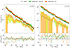 |
Fig. 2. Top: Comparison of the PINOCCHIO covariance of the 2PCF measured on the comoving box from the original mocks (Fumagalli et al. 2021) and our new high-resolution C0. Similarly to Fig. 1, we present only the theoretical expectation from the baseline model presented in Eq. (3) for the C0 cosmology for better figure readability. Bottom: Residual between the measured 2PCF and the respective theoretical expectation. In both panels, darker colors are used for diagonal and lighter for the first off-diagonal terms. |
To assess the impact of the resolution on the PINOCCHIO predictions, in Fig. 3 we compare the bias (b) and shot-noise correction (α) measured from the new 100 C0 simulations at higher resolution with respect to the 20 simulations with same cosmology but lower resolution. The measurements are from the outputs in comoving boxes at different redshifts and with different minimum mass selection Mcut∈{1014, 3×10¹⁴} M⊙ h−1. We measured the bias from the ratio of the cross-spectrum Ph, m between the halo and matter to the matter-power spectrum, Pm. The shot-noise correction α is measured using the following relation
 (5)
(5)
where  is the mean density of halos.
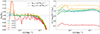 |
Fig. 3. Comparison of resolution effects on PINOCCHIO predictions for halo bias, b(k) (left) and shot-noise correction, α(k) (right). We show the ratio between high-resolution (HR; 100 C0 simulations) and low-resolution (LR; 20 simulations) results at redshifts z∈{0.0, 0.5, 1.0, 2.0} for two mass thresholds: Mcut = 1014 M⊙ h−1 (solid) and Mcut = 3×10¹⁴ M⊙ h−1 (dashed). While bias differences remain below 2 percent for z≤1.0, reaching 5 percent at z = 2 (the larger mass cut case is omitted for z = 2 due to noise), the shot-noise corrections converge within 10 percent for z≤1 but show 30 percent deviations at z = 2. |
We observe in Fig. 3 that the differences in the bias due to resolution are more minor than 2 percent for the different mass and redshift selections, except the redshift two, where differences are roughly 5 percent for 1014 M⊙ h−1 mass selection. The case for the mass selection of 3×10¹⁴ M⊙ h−1 is not shown for redshift two as, in this case, the measurements are very noisy due to the small number of tracers. Concerning the shot-noise correction, α, we observe that the original simulations converge within a few percent for redshifts below unity. For redshift z = 1, while the measurements from the 1014 M⊙ h−1 still agree within said accuracy, for the 3×10¹⁴ M⊙ h−1, we observe a difference on the order of 10 percent. The differences can be as significant as 30 percent for the case of redshift z = 2. This indicates that the original resolution might be too low to calibrate the shot-noise correction accurately at high redshifts.
We note that the parameters α and β in the covariance model have slightly different meanings and values compared to those fitted from the power spectrum. This is because the three covariance parameters also absorb the effects of missing higher-order terms in the covariance, partially losing their physical interpretation (Euclid Collaboration: Fumagalli et al. 2024). The agreement between these parameters will be discussed in Sect. 4.2.
4.2. OpenGADGET3 versus PINOCCHIO
In Fig. 4 we compare the effective halo bias measured from the mass-scaled catalogs produced by OpenGADGET3 and PINOCCHIO (set 3) to the theoretical prediction from Euclid Collaboration: Castro et al. (2024). Overall, OpenGADGET3 and PINOCCHIO agree at the 5–10% level for most scales and redshifts, but at higher redshifts (particularly z = 2.0) and for larger mass cuts, we observe slightly larger deviations. These differences between the codes reflect residual nonlinearities or shot-noise corrections not fully captured by the mass-scaling procedure.
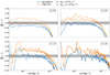 |
Fig. 4. Comparison between the effective bias from mass-scaled halo catalogs from OpenGADGET3 and PINOCCHIO and the theoretical expectation from Euclid Collaboration: Castro et al. (2024). Different panels show the results for different redshifts corresponding to {0.0, 0.5, 1.0, 2.0}, going clockwise. Different line styles correspond to different minimum mass selections. We omit the result for the Mcut = 3×10¹⁴ h−1 M⊙ at z = 2 as the measurements are too noisy due to the low statistics. |
In Fig. 5 we compare the non-Poissonian correction to the shot noise, α(k), for the same halo catalogs. We find that OpenGADGET3 and PINOCCHIO exhibit broadly similar trends in α(k), remaining close to zero for large scales and high redshifts but displaying noticeable deviations for high masses and lower redshifts.
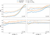 |
Fig. 5. Comparison between the non-Poissonian correction to the shot noise of the mass-scaled halo catalogs from OpenGADGET3 and PINOCCHIO. Different panels show the results for different redshifts corresponding to {0.0, 0.5, 1.0, 2.0}, going clockwise. Different lifestyles correspond to different minimum mass selections. |
Figures 4 and 5 highlight that, when using the same initial phases and a consistent mass-scaling scheme, OpenGADGET3 and PINOCCHIO reproduce the large-scale bias and shot-noise properties of halo catalogs to within a few percent in most regimes. These results suggest that our mass-scaling procedure effectively aligns the mass functions between OpenGADGET3 and PINOCCHIO. Still, subtle discrepancies remain, likely reflecting that the scaling procedure does not consider each cluster's environment.
Figure 6 presents the posterior distributions of the parameters α, β, and γ from Eq. (4), derived by fitting the 2PCF covariance measured in the comoving boxes for OpenGADGET3 (set 2) and PINOCCHIO (set 1). Overall, we observe good agreement between the two codes for both mass cuts. The values of α and γ are broadly consistent across the different simulations, reflecting similar levels of non-Poissonian noise corrections and sub-leading shot-noise contributions. A slight offset emerges in β, with PINOCCHIO typically favoring higher values than OpenGADGET3, in line with the differences in the practical bias seen in Fig. 4. This offset suggests that the PINOCCHIO halos may require a larger rescaling of the bias to reproduce the measured covariance, possibly reflecting the limitations of the approximated method. Nonetheless, the overlap in the posterior contours for all parameters indicates that the two approaches yield broadly consistent covariance calibrations. Evidence of this can be observed in Fig. 7, which compares the numerical and semi-analytical covariances for OpenGADGET3 and PINOCCHIO, using best-fit parameters from Fig. 6. The residuals between the two models show agreement within 5% in most cases, except for off-diagonal terms at z = 1. However, these terms are subdominant and do not significantly impact cosmological analysis. Such a result reinforces the conclusion that PINOCCHIO can reliably match OpenGADGET3 covariance results with an appropriate mass-scaling procedure and modest adjustments of the nuisance parameters.
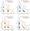 |
Fig. 6. Posteriors for fitted covariance parameters: PINOCCHIO vs. OpenGADGET3 for the C0 cosmology for redshifts z = 0 (left) and z = 1 (right) and masses M>1014 h−1 M⊙ (top) and M>3×10¹⁴ h−1 M⊙ (bottom). |
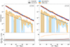 |
Fig. 7. Covariance comparison (box): PINOCCHIO vs. OpenGADGET3 covariance matrices, at z = 0 (left panel) and z = 1 (right panel). Shaded areas represent the numerical covariance within 1σ uncertainty, and solid lines are the semi-analytical prediction, with fitted parameters. Orange colors indicate PINOCCHIO covariance, while blue colors are for OpenGADGET3. Darker colors represent the diagonal terms, lighter colors the first off-diagonal terms. Bottom panels show the residuals of the PINOCCHIO fitted model with respect to the OpenGADGET3 one (solid line for the diagonal elements, dashed line for the off-diagonal ones). |
We also find that fitting the covariance parameters using 100 mocks yields stable results up to 25 separation bins within our chosen radial range. Although this is not a universal criterion, more than 100 simulations may be required if a finer binning scheme is used.
4.3. Cosmological dependence
In Fig. 8 we show the best-fit values for the covariance model from Eq. (4) as a function of cosmology. For a more realistic comparison, we performed the fit using light cones divided into different redshift bins. The parameter α, while staying within the range [−0.05, 0.15] – indicating small deviations from Poissonian shot noise – tends to increase with σ8, suggesting a mild linear dependence on the amplitude of matter fluctuations. By contrast, β (the bias rescaling) and γ (the sub-leading shot-noise correction) do not show a strong trend with σ8. However, both β and γ exhibit noticeable variations with redshift. Specifically, β remains in the range [1.0, 1.5] for the different cosmologies but shifts slightly across redshift bins. At the same time, γ is negative for most cosmologies, implying that the baseline Poisson noise may be an overestimate of the actual sampling noise in specific regimes but tends to decrease with increasing redshift. These results emphasize that even though the global amplitude of non-Poissonian effects and bias corrections is small, allowing flexible parameters in the covariance model is essential for capturing the redshift dependences and subtle but nontrivial responses to variations in σ8.
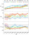 |
Fig. 8. Best-fit covariance-model parameters α (top panel), β (middle panel), and γ (bottom panel) as a function of cosmology. Each color corresponds to a different redshift bin |

Additionally, the amplitude of β typically exceeds the observed accuracy of PINOCCHIO in reproducing the linear bias, suggesting that β may absorb extra flexibility beyond merely correcting the bias (e.g., mild nonlinearities). Furthermore, the redshift dependence of both β and γ indicates that these parameters are sensitive to the survey selection function. Consequently, when applying the model to cosmological data, one should calibrate these parameters on realistic mocks that replicate the actual selection function, ensuring that the resulting covariance matrix accurately captures both the intrinsic clustering of the sample and the observational selection effects.
Although we show the results for increasing σ8, we also analyzed the residual dependence as a function of Ωm and the composite variable  . While α shows some small dependence on S8, it is less significant than the dependence on σ8; the other parameters do not show any considerable dependence.
The dependence of the non-Poissonian correction primarily on σ8 and not on S8 is indicative that the clustering amplitude of the underlying density field is the physical mechanism behind it and not the number density of halos of a given mass, which is instead determined by S8. Nonlinear clustering indeed introduces correlations between the fluctuations in the halo number density that could be reflected in the deviation of the density field sampling provided by halos from a standard Poisson sampling. A thorough study of this issue deserves a dedicated analysis that goes beyond the scope of this work.
5. Discussion
Approximate methods, and in the specific case of this paper, the PINOCCHIO code, have become a valuable tool in cosmology by providing results in a fraction of the time required by full N-body simulations (Chuang et al. 2015; Monaco 2016). However, this efficiency is achieved by compromising the accuracy with which the underlying statistical properties are reproduced. Different papers have shown that PINOCCHIO nominal accuracy for different statistics, including subhalo clustering data (Berner et al. 2022) and full-sky 21 cm intensity mapping mocks (Hitz et al. 2024), is roughly 10 percent. Due to its efficiency, PINOCCHIO is a natural candidate to generate massive synthetic data needed to extract the covariance of different cluster statistics numerically (Fumagalli et al. 2021; Euclid Collaboration: Fumagalli et al. 2024). However, as shown by Sellentin & Starck (2019), approximate covariance matrices might bias cosmological constraints and, therefore, should be treated at equal footing with the signal modeling to ensure an unbiased analysis.
In this paper, we have focused on the cluster clustering covariance. Euclid Collaboration: Fumagalli et al. (2024) show that the low-order analytical model of Meiksin & White (1999) does not quantitatively reproduce the numerical covariance extracted from PINOCCHIO catalogs. Euclid Collaboration: Fumagalli et al. (2024) proposed a semi-analytical extension, presented in Sect. 2. The proposed model could reproduce the covariance accurately if the free parameters α, β, and γ appearing in Eq. (4) were appropriately calibrated (Fumagalli et al. 2022). Therefore, it is important to assess the resolution, cosmological, and methodological impacts on the calibration of these parameters.
The parameters α and β are related to the shot-noise correction to the Poisson expectation and residual errors on the linear bias. The non-Poissonian correction can be measured from the simulations using the matter, halo, and matter-halo power spectrum using the estimator presented in Eq. (5). The need for a bias correction can be assessed by comparing the halo bias, as measured from the ratio of the matter-halo cross-spectrum and matter power spectrum at linear scales, concerning the fiducial linear bias model (Euclid Collaboration: Castro et al. 2024). In Sect. 4.1 we show that a mass resolution of approximately 6×10¹¹ h−1 M⊙ for PINOCCHIO is too low to produce convergent results for α and β, especially at higher redshifts, compared to a simulation that has a factor of 4 more resolution elements.
Regarding the comparison between PINOCCHIO and OpenGADGET3, in Sect. 4.2 we show that the shot-noise correction displays similar trends in the two codes. However, the overall amplitude of the shot-noise correction (i.e., 1+α) differs by as much as 10 percent. In contrast, for the bias correction β, PINOCCHIO systematically overpredicts the value relative to OpenGADGET3, with a stable relative difference of approximately 5 percent that could be easily corrected during calibration. Correcting this slight bias would yield an even better agreement between the calibrations of PINOCCHIO and OpenGADGET3. Nevertheless, even without such a correction, the covariances obtained from both codes remain statistically equivalent within the uncertainties assessed in this work.
Furthermore, regarding the cosmological dependence of the parameters, only α shows a small dependence with σ8. While the linear coefficients of said relation do not show a redshift dependence, its normalization decreases with redshift over the redshift range z = [0–1] and is constant at higher redshifts.
Lastly, for both PINOCCHIO and OpenGADGET3 we observe that the extra parameters α, β, and γ depend on redshift and mass cuts. This dependence implies that the final covariance depends on the selection function. Therefore, future cosmological analysis should use mock catalogs that mimic the sample selection function.
6. Conclusions
In this paper we have assessed the robustness of the calibration of the semi-analytical model for the 2PCF covariance on both fast approximate PINOCCHIO and OpenGADGET3 N-body simulations across multiple cosmological models. We summarize our main findings:
-
–
The shot-noise corrections and bias calibration converge more reliably in higher-resolution PINOCCHIO simulations (Mpart.≲1011 h−1 M⊙), particularly at z≳1. We observe that insufficient mass resolution can bias the non-Poissonian shot-noise parameter by up to 30%.
-
–
When started from the same initial random field, PINOCCHIO and OpenGADGET3 yield broadly consistent covariance estimates for the cluster 2PCF. Small discrepancies at the 5–10% level can be accounted for by modest shifts in the model's nuisance parameters (see Eq. (4)). This demonstrates that PINOCCHIO can provide a reliable and computationally efficient alternative to full N-body simulations when measuring clustering covariances for large cosmological surveys of galaxy clusters.
-
–
Of the three calibrated nuisance parameters, only the non-Poissonian shot-noise correction, α, shows a mild linear dependence on σ8. The other parameters, β (bias rescaling) and γ (sub-leading shot-noise correction), exhibit more pronounced redshift and mass cut dependences than cosmology dependence.
-
–
The redshift and mass cuts and redshift dependences indicate that the survey selection function impacts the covariance calibration. Accurate modeling of the covariance for application to specific surveys thus requires realistic mocks that replicate the observed selection to avoid systematic biases in cosmological inference.
Overall, our results confirm that this semi-analytical covariance model can robustly capture the main sources of uncertainty in cluster clustering, provided the nuisance parameters are carefully tuned. In particular, approximate simulations such as PINOCCHIO can be employed effectively for such a calibration, enabling robust covariance estimates across diverse cosmological models and redshifts without incurring the computational expense of full N-body simulations. Furthermore, the demonstrated success of PINOCCHIO in reproducing the cluster covariance motivates the extension of our analysis to a multi-probe context in future studies. Importantly, assessing its capability to estimate covariances for additional cluster-based summary statistics, such as cluster shear correlation and cluster galaxy correlation, will allow a more comprehensive evaluation of approximate methods in various cosmological applications.
Data availability
The numerical data generated and analyzed in this study are not publicly available due to the large storage and computational resources required. The authors will make every reasonable effort to provide access to the underlying simulation outputs and derived data products upon request, subject to resource availability. The fiducial models for the HMF and halo bias used in this paper can be accessed in Castro & Fumagalli (2024)9.
Acknowledgments
The authors A. Fumagalli and T. Castro share co-authorship of this paper. T. Castro conceptualized and produced the simulated data, while A. Fumagalli carried out the formal analysis of the simulated data. All authors contributed to interpreting the results and writing the manuscript. All authors have read and approved the final version of the paper. It is a pleasure to thank Isabella Baccarelli, Fabio Pitari, and Caterina Caravita for their support with the CINECA environment. This work is supported by the Agenzia Spaziale Italiana (ASI) under – Euclid-FASE D Attivita’ scientifica per la missione – Accordo attuativo ASI-INAF n. 2018-23-HH.0, by the National Recovery and Resilience Plan (NRRP), Mission 4, Component 2, Investment 1.1, Call for tender No. 1409 published on 14.9.2022 by the Italian Ministry of University and Research (MUR), funded by the European Union – NextGenerationEU – Project Title “Space-based cosmology with Euclid: the role of High-Performance Computing” – CUP J53D23019100001 – Grant Assignment Decree No. 962 adopted on 30/06/2023 by the Italian Ministry of Ministry of University and Research (MUR); by the Italian Research Center on High-Performance Computing Big Data and Quantum Computing (ICSC), a project funded by the European Union – NextGenerationEU – and National Recovery and Resilience Plan (NRRP) – Mission 4 Component 2, by the INFN INDARK PD51 grant, and by the PRIN 2022 project EMC2 – Euclid Mission Cluster Cosmology: unlock the full cosmological utility of the Euclid photometric cluster catalog (code no. J53D23001620006). AF acknowledges support by the Excellence Cluster ORIGINS, which is funded by the Deutsche Forschungsgemeinschaft (DFG, German Research Foundation) under Germany's Excellence Strategy – EXC-2094 – 390783311. AF acknowledges support from the Ludwig-Maximilians-Universität in Munich. The simulations were run partially on the Leonardo-Booster supercomputer as part of the Leonardo Early Access Program (LEAP) and under the ISCRA initiative. We acknowledge the CINECA award for the availability of high-performance computing resources and support. We acknowledge the use of the HOTCAT computing infrastructure of the Astronomical Observatory of Trieste – National Institute for Astrophysics (INAF, Italy) (see Bertocco et al. 2020; Taffoni et al. 2020).
References
- Allen, S. W., Evrard, A. E., & Mantz, A. B. 2011, ARA&A, 49, 409 [Google Scholar]
- Benson, B. A., Ade, P. A. R., Ahmed, Z., et al. 2014, Proc. SPIE Int. Soc. Opt. Eng., 9153, 91531P [Google Scholar]
- Berner, P., Refregier, A., Sgier, R., et al. 2022, JCAP, 11, 002 [Google Scholar]
- Bertocco, S., Goz, D., Tornatore, L., et al. 2020, ASP Conf. Ser., 527, 303 [NASA ADS] [Google Scholar]
- Bocquet, S., Dietrich, J. P., Schrabback, T., et al. 2019, ApJ, 878, 55 [Google Scholar]
- Borgani, S., Rosati, P., Tozzi, P., et al. 2001, ApJ, 561, 13 [NASA ADS] [CrossRef] [Google Scholar]
- Castro, T., & Fumagalli, A. 2024, https://doi.org/10.5281/zenodo.13485873, https://github.com/TiagoBsCastro/CCToolkit [Google Scholar]
- Castro, T., Borgani, S., Dolag, K., et al. 2020, MNRAS, 500, 2316 [Google Scholar]
- Chuang, C. -H., Zhao, C., Prada, F., et al. 2015, MNRAS, 452, 686 [CrossRef] [Google Scholar]
- Cohn, J. D. 2006, New Astron., 11, 226 [NASA ADS] [CrossRef] [Google Scholar]
- Costanzi, M., Saro, A., Bocquet, S., et al. 2021, PRD, 103, 043522 [NASA ADS] [CrossRef] [Google Scholar]
- Davis, M., Efstathiou, G., Frenk, C. S., & White, S. D. M. 1985, ApJ, 292, 371 [Google Scholar]
- DESI Collaboration (Aghamousa, A., et al.) 2016, arXiv e-prints [arXiv:arXiv:1611.00036] [Google Scholar]
- Dolag, K., Borgani, S., Murante, G., & Springel, V. 2009, MNRAS, 399, 497 [Google Scholar]
- Euclid Collaboration (Castro, T., et al.) 2023, A&A, 671, A100 [CrossRef] [EDP Sciences] [Google Scholar]
- Euclid Collaboration (Castro, T., et al.) 2024, A&A, 691, A62 [Google Scholar]
- Euclid Collaboration (Fumagalli, A., et al.) 2024, A&A, 683, A253 [NASA ADS] [CrossRef] [EDP Sciences] [Google Scholar]
- Euclid Collaboration (Mellier, Y., et al.) 2025, A&A, 697, A1 [Google Scholar]
- Fumagalli, A., Saro, A., Borgani, S., et al. 2021, A&A, 652, A21 [NASA ADS] [CrossRef] [EDP Sciences] [Google Scholar]
- Fumagalli, A., Biagetti, M., Saro, A., et al. 2022, JCAP, 12, 022 [Google Scholar]
- Fumagalli, A., Costanzi, M., Saro, A., Castro, T., & Borgani, S. 2024, A&A, 682, A148 [NASA ADS] [CrossRef] [EDP Sciences] [Google Scholar]
- Hitz, P., Berner, P., Crichton, D., Hennig, J., & Refregier, A. 2024, arXiv e-prints [arXiv:arXiv:2410.01694] [Google Scholar]
- Hu, W., & Kravtsov, A. V. 2003, ApJ, 584, 702 [Google Scholar]
- Kravtsov, A., & Borgani, S. 2012, ARA&A, 50, 353 [NASA ADS] [CrossRef] [Google Scholar]
- Landy, S. D., & Szalay, A. S. 1993, ApJ, 412, 64 [Google Scholar]
- Laureijs, R., Amiaux, J., Arduini, S., et al. 2011, arXiv e-prints [arXiv:arXiv:1110.3193] [Google Scholar]
- LSST Science Collaborations (Abell, P. A., et al.) 2009, arXiv e-prints [arXiv:arXiv:0912.0201] [Google Scholar]
- Maartens, R., Abdalla, F. B., Jarvis, M., & Santos, M. G. 2015, PoS, AASKA14, 016 [Google Scholar]
- Majumdar, S., & Mohr, J. J. 2004, ApJ, 613, 41 [NASA ADS] [CrossRef] [Google Scholar]
- Mana, A., Giannantonio, T., Weller, J., et al. 2013, MNRAS, 434, 684 [NASA ADS] [CrossRef] [Google Scholar]
- Marulli, F., Veropalumbo, A., & Moresco, M. 2016, Astron. Comput., 14, 35 [Google Scholar]
- Marulli, F., Veropalumbo, A., Sereno, M., et al. 2018, A&A, 620, A1 [NASA ADS] [CrossRef] [EDP Sciences] [Google Scholar]
- Meiksin, A., & White, M. J. 1999, MNRAS, 308, 1179 [NASA ADS] [CrossRef] [Google Scholar]
- Michaux, M., Hahn, O., Rampf, C., & Angulo, R. E. 2021, MNRAS, 500, 663 [Google Scholar]
- Monaco, P. 2016, Galaxies, 4, 53 [NASA ADS] [CrossRef] [Google Scholar]
- Monaco, P., Theuns, T., & Taffoni, G. 2002, MNRAS, 331, 587 [Google Scholar]
- Monaco, P., Sefusatti, E., Borgani, S., et al. 2013, MNRAS, 433, 2389 [NASA ADS] [CrossRef] [Google Scholar]
- Munari, E., Monaco, P., Sefusatti, E., et al. 2017, MNRAS, 465, 4658 [Google Scholar]
- Planck Collaboration XX. 2014, A&A, 571, A20 [NASA ADS] [CrossRef] [EDP Sciences] [Google Scholar]
- Planck Collaboration XXIV. 2016, A&A, 594, A24 [NASA ADS] [CrossRef] [EDP Sciences] [Google Scholar]
- Predehl, P., Andritschke, R., Arefiev, V., et al. 2021, A&A, 647, A1 [EDP Sciences] [Google Scholar]
- Sartoris, B., Biviano, A., Fedeli, C., et al. 2016, MNRAS, 459, 1764 [Google Scholar]
- Schuecker, P., Bohringer, H., Collins, C. A., & Guzzo, L. 2003, A&A, 398, 867 [NASA ADS] [CrossRef] [EDP Sciences] [Google Scholar]
- Scoccimarro, R., Zaldarriaga, M., & Hui, L. 1999, ApJ, 527, 1 [NASA ADS] [CrossRef] [Google Scholar]
- Sellentin, E., & Starck, J. -L. 2019, JCAP, 08, 021 [Google Scholar]
- Spergel, D., Gehrels, N., Baltay, C., et al. 2015, arXiv e-prints [arXiv:arXiv:1503.03757] [Google Scholar]
- Springel, V. 2005, MNRAS, 364, 1105 [Google Scholar]
- Springel, V., White, S. D. M., Tormen, G., & Kauffmann, G. 2001, MNRAS, 328, 726 [Google Scholar]
- Springel, V., Pakmor, R., Zier, O., & Reinecke, M. 2021, MNRAS, 506, 2871 [NASA ADS] [CrossRef] [Google Scholar]
- Taffoni, G., Becciani, U., Garilli, B., et al. 2020, ASP Conf. Ser., 527, 307 [NASA ADS] [Google Scholar]
- Takada, M., & Hu, W. 2013, PRD, 87, 123504 [Google Scholar]
- To, C. -H., et al. 2021, MNRAS, 502, 4093 [NASA ADS] [CrossRef] [Google Scholar]
- Vikhlinin, A., Kravtsov, A. V., Burenin, R. A., et al. 2009, ApJ, 692, 1060 [Google Scholar]
- Watson, W. A., Iliev, I. T., D’Aloisio, A., et al. 2013, MNRAS, 433, 1230 [Google Scholar]
All Tables
All Figures
|
Fig. 1. Top: Comparison of the PINOCCHIO 2PCF measured on the comoving box from the original mocks (Fumagalli et al. 2021) and our new high-resolution C0. The new and original simulations assume different but similar cosmologies. We present only the theoretical expectation for the C0 cosmology for better figure readability. Bottom: Residual between the measured 2PCF and the respective theoretical expectation. The shaded gray area denotes the region within a relative difference of less than 10 percent. |
| In the text | |
|
Fig. 2. Top: Comparison of the PINOCCHIO covariance of the 2PCF measured on the comoving box from the original mocks (Fumagalli et al. 2021) and our new high-resolution C0. Similarly to Fig. 1, we present only the theoretical expectation from the baseline model presented in Eq. (3) for the C0 cosmology for better figure readability. Bottom: Residual between the measured 2PCF and the respective theoretical expectation. In both panels, darker colors are used for diagonal and lighter for the first off-diagonal terms. |
| In the text | |
|
Fig. 3. Comparison of resolution effects on PINOCCHIO predictions for halo bias, b(k) (left) and shot-noise correction, α(k) (right). We show the ratio between high-resolution (HR; 100 C0 simulations) and low-resolution (LR; 20 simulations) results at redshifts z∈{0.0, 0.5, 1.0, 2.0} for two mass thresholds: Mcut = 1014 M⊙ h−1 (solid) and Mcut = 3×10¹⁴ M⊙ h−1 (dashed). While bias differences remain below 2 percent for z≤1.0, reaching 5 percent at z = 2 (the larger mass cut case is omitted for z = 2 due to noise), the shot-noise corrections converge within 10 percent for z≤1 but show 30 percent deviations at z = 2. |
| In the text | |
|
Fig. 4. Comparison between the effective bias from mass-scaled halo catalogs from OpenGADGET3 and PINOCCHIO and the theoretical expectation from Euclid Collaboration: Castro et al. (2024). Different panels show the results for different redshifts corresponding to {0.0, 0.5, 1.0, 2.0}, going clockwise. Different line styles correspond to different minimum mass selections. We omit the result for the Mcut = 3×10¹⁴ h−1 M⊙ at z = 2 as the measurements are too noisy due to the low statistics. |
| In the text | |
|
Fig. 5. Comparison between the non-Poissonian correction to the shot noise of the mass-scaled halo catalogs from OpenGADGET3 and PINOCCHIO. Different panels show the results for different redshifts corresponding to {0.0, 0.5, 1.0, 2.0}, going clockwise. Different lifestyles correspond to different minimum mass selections. |
| In the text | |
|
Fig. 6. Posteriors for fitted covariance parameters: PINOCCHIO vs. OpenGADGET3 for the C0 cosmology for redshifts z = 0 (left) and z = 1 (right) and masses M>1014 h−1 M⊙ (top) and M>3×10¹⁴ h−1 M⊙ (bottom). |
| In the text | |
|
Fig. 7. Covariance comparison (box): PINOCCHIO vs. OpenGADGET3 covariance matrices, at z = 0 (left panel) and z = 1 (right panel). Shaded areas represent the numerical covariance within 1σ uncertainty, and solid lines are the semi-analytical prediction, with fitted parameters. Orange colors indicate PINOCCHIO covariance, while blue colors are for OpenGADGET3. Darker colors represent the diagonal terms, lighter colors the first off-diagonal terms. Bottom panels show the residuals of the PINOCCHIO fitted model with respect to the OpenGADGET3 one (solid line for the diagonal elements, dashed line for the off-diagonal ones). |
| In the text | |
|
Fig. 8. Best-fit covariance-model parameters α (top panel), β (middle panel), and γ (bottom panel) as a function of cosmology. Each color corresponds to a different redshift bin |
| In the text | |
Current usage metrics show cumulative count of Article Views (full-text article views including HTML views, PDF and ePub downloads, according to the available data) and Abstracts Views on Vision4Press platform.
Data correspond to usage on the plateform after 2015. The current usage metrics is available 48-96 hours after online publication and is updated daily on week days.
Initial download of the metrics may take a while.